Abstract

The Hosoya polynomial is a well known vertex-distance based polynomial, closely correlated to the Wiener index and the hyper-Wiener index, which are widely used molecular-structure descriptors. In the present paper we consider the edge version of the Hosoya polynomial. For a connected graph $G$ let $d_{e}(G,k)$ be the number of (unordered) edge pairs at distance $k$ . Then the edge-Hosoya polynomial of $G$ is $H_{e}(G,x)=\sum_{k\geq 0}d(G,k)\,x^{k}$ . We investigate the edge-Hosoya polynomial of important chemical graphs known as benzenoid chains and derive the recurrence relations for them. These recurrences are then solved for linear benzenoid chains, which are also called polyacenes.

1 Introduction

In 1988 H. Hosoya introduced some counting polynomials in chemistry [7], among them the Wiener polynomial, nowadays known as the Hosoya polynomial. Since then the topic has been intensively researched - for example, the Hosoya polynomial of benzenoid chains [6, 17], carbon nanotubes [18], circumcoronene series [14], Finonacci and Lucas cubes [12] has been calculated. For some recent results on the Hosoya polynomial see [5]. What makes the Hosoya polynomial interesting in chemistry is especially the strong connection to the Wiener index and the hyper-Wiener index [2].

The Hosoya polynomial is based on the distances between pairs of vertices in a graph, and similar concept has been introduced in [1] for distances between pairs of edges under the name the edge-Hosoya polynomial. The authors defined the distance between two edges $e=ab$ and $f=xy$ of a graph $G$ as $\widehat{d}(e,f)=\min\{d(a,x),d(a,y),d(b,x),d(b,y)\}$. However, the distance between two edges of graph $G$ can also be defined as the distance between vertices $e$ and $f$ in the line graph $L(G)$. In [8] it was discussed that the pair $(E(G),\widehat{d})$ is not a metric space and therefore it was suggested that the distance between pairs of edges should be considered in the line graph. Hence, in the present paper we use the last definition of distance between edges for the edge-Hosoya polynomial $H_{e}(G,x)$. The other version of the edge-Hosoya polynomial using distance $\widehat{d}$ is denoted by $\widehat{H}_{e}(G,x)$. In [1] the relation between both versions of the edge-Hosoya polynomial was established, but it is not completely correct. In the present paper the true relation is proved in Proposition 2.2. Moreover, the relation between the Hosoya polynomial and the edge-Hosoya polynomial for trees was established in [16].

Next, we describe the strong connections of the edge-Hosoya polynomial to the edge-Wiener index and the edge-hyper-Wiener index, which show the importance of the edge-Hosoya polynomial in chemistry. The edge-Wiener index [8] and the edge-hyper-Wiener index [9] of a connected graph $G$ are defined as

$$W_{e}(G)=\frac{1}{2}\sum_{e\in E(G)}\sum_{f\in E(G)}d(e,f),$$

$$WW_{e}(G)=\frac{1}{4}\sum_{e\in E(G)}\sum_{f\in E(G)}d(e,f)+\frac{1}{4}\sum_{e\in E(G)}\sum_{f\in E(G)}d(e,f)^{2}$$

and have been much investigated in recent years (for example, see [3, 4, 10, 13, 15]). The equality

$$W_{e}(G)=H_{e}^{\prime}(G,1)$$ (1)

between the edge-Wiener index and the edge-Hosoya polynomial is obvious and the equality between the edge-hyper-Wiener index and the edge-Hosoya polynomial was shown in [16]:

$$WW_{e}(G)=H_{e}^{\prime}(G,1)+\frac{1}{2}H_{e}^{\prime\prime}(G,1).$$ (2)

The main aim of the paper is deriving the recursive relations of the edge-Hosoya polynomial for benzenoid chains. This continues the research from [6], where similar methods were used for determining the Hosoya polynomial. However, in our case some additional recursions are needed. In the next section we introduce basic concepts and the relation between $H_{e}(G,x)$ and $\widehat{H}_{e}(G,x)$ is established. In sections 3 and 4 the recursive relations for the edge-Hosoya polynomial of benzenoid chains are calculated and solved for polyacenes in the final section. In a similar way, the edge-Hosoya polynomial can be computed for any benzenoid chain.

2 Preliminaries

Distance $d(x,y)$ between vertices $x,y\in V(G)$ is defined as the usual shortest-path distance. If $G$ is a connected graph and if $d_{v}(G,k)$ is the number of (unordered) pairs of its vertices that are at distance $k$ , then the Hosoya polynomial of $G$ is defined as

$$H(G,x)=\sum_{k\geq 0}d_{v}(G,k)\,x^{k}.$$

The distance between edges $e$ and $f$ of a graph $G$, $d(e,f)$, is defined as the distance between vertices $e$ and $f$ in the line graph $L(G)$. The distance between a vertex $w$ and an edge $e=uv$ is defined as $d(w,e)=\min\{d(w,u),d(w,v)\}$.

If $G$ is a connected graph with $m$ edges, and if $d_{e}(G,k)$ is the number of (unordered) pairs of its edges that are at distance $k$ , then the edge-Hosoya polynomial of $G$ is

$$H_{e}(G,x)=\sum_{k\geq 0}d_{e}(G,k)\,x^{k}.$$

For convenience we write $d(G,k)$ for $d_{e}(G,k)$ and set $d(G,k)=0$ for $k<0$. Note that $d(G,0)=m$. Also, the following proposition is obvious.

Proposition 2.1

Let $G$ be a connected graph. Then

$$H_{e}(G,x)=H(L(G),x).$$

On the other hand, for edges $e=ab$ and $f=xy$ of a graph $G$ it is also legitimate to set

$$\widehat{d}(e,f)=\min\{d(a,x),d(a,y),d(b,x),d(b,y)\}\,.$$

Replacing $d$ with $\widehat{d}$, a variant of the edge-Hosoya polynomial from [1] is obtained, let us denote it with $\widehat{H}_{e}(G,x)$. The following proposition gives us the relation between both variants of the edge-Hosoya polynomial. Similar result was also obtained in [1] as Theorem $1$, but there it is not completely correct.

Proposition 2.2

Let $G$ be a connected graph. Then

$$H_{e}(G,x)=x\left(\widehat{H}_{e}(G,x)-|E(G)|\right)+|E(G)|.$$

Proof.  If $k=0$, then it is obvious that $d(G,0)=|E(G)|$. Let $k=1$. The number $d(G,1)$ is equal to the number of pairs of edges $e$ and $f$ such that $d(e,f)=1$. However, it follows that $d(G,1)$ is the number of pairs of edges $e$ and $f$ for which $\widehat{d}(e,f)=0$, reduced by the number of edges of $G$, $|E(G)|$. Therefore, the coefficient before $x^{1}$ is the same on the both sides. Finally, let $k>1$. Then $d(G,k)$ is equal to the number of pairs of edges $e$ and $f$ for which $d(e,f)=\widehat{d}(e,f)+1=k$, therefore, the coefficient before $x^{k}$ in $H_{e}(G,x)$ is equal to the coefficient before $x^{k-1}$ in $\widehat{H}_{e}(G,x)$. The proof is complete. $\square$

Finally, we need some additional definitions. For a graph $G$ , $k\geq 0$ , and a vertex $v\in V(G)$ , let $d(G,v,k)$ be the number of edges of $G$ at distance $k$ from $v$ . This time, $d(G,v,0)=deg(v)$ , and for $k<0$ we set $d(G,v,k)=0$ . We now define $H_{e}(G,v,x)$ as

$$H_{e}(G,v,x)=\sum_{k\geq 0}d(G,v,k)x^{k}\ .$$

For a graph $G$ , $k\geq 0$ , and an edge $e\in E(G)$ , let $d(G,e,k)$ be the number of edges of $G$ at distance $k$ from $e$ . This time, $d(G,e,0)=1$ , and for $k<0$ we set $d(G,e,k)=0$ . We now define $H_{e}(G,e,x)$ as

$$H_{e}(G,e,x)=\sum_{k\geq 0}d(G,e,k)x^{k}\ .$$

3 Annelating a $6$-cycle

In this section we describe how the edge-Hosoya polynomial of a graph $G_{0}$ can be used to compute the edge-Hosoya polynomial of a graph $G$, obtained by attaching a $6$-cycle to $G_{0}$. In chemistry, such an operation is known as annelation. The obtained result will be used in the next section, where we consider benzenoid chains.

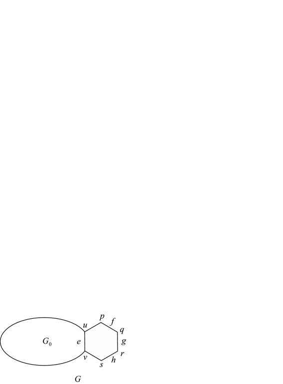
Figure 1: A graph $G$ obtained by annelating a $6$-cycle to $G_{0}$ over an edge $e=uv$.

Theorem 3.1

Let the graph $G$ be obtained by annelating a $6$-cycle to the graph $G_{0}$ over an edge $e=uv$. Then

$$H_{e}(G,x) = H_{e}(G_{0},x)+(x+x^{2})H_{e}(G_{0},u,x)+(x+x^{2})H_{e}(G_{0},v,x)$$

$$+ x^{2}H_{e}(G_{0},e,x)+5+4x+3x^{2}+3x^{3}.$$

Proof.  Let $e$, $u$ and $v$ be as in the Figure 1 and $k$ an integer. We define $d(G_{0},k,e,u,v)$ as the sum

$$d(G_{0},k)+d(G_{0},u,k-1)+d(G_{0},u,k-2)+d(G_{0},v,k-1)+d(G_{0},v,k-2)+d(G_{0},e,k-2).$$

Obviously, it follows from Figure 1, that for every $k\geq 0$ it holds

$$d(G,k)=d(G_{0},k,e,u,v)+\left\{\begin{array}[]{ll}0\ ;&k>3\\ 3\ ;&k=3\\ 3\ ;&k=2\\ 4\ ;&k=1\\ 5\ ;&k=0.\end{array}\right.$$

Therefore,

$$H_{e}(G,x)=\sum_{k\geq 0}d(G,k)=\sum_{k\geq 0}d(G_{0},k,e,u,v)+5+4x+3x^{2}+3x^{3},$$

which implies

$$H_{e}(G,x) = H_{e}(G_{0},x)+xH_{e}(G_{0},u,x)+x^{2}H_{e}(G_{0},u,x)$$

$$+ xH_{e}(G_{0},v,x)+x^{2}H_{e}(G_{0},v,x)+x^{2}H_{e}(G_{0},e,x)$$

$$+ 5+4x+3x^{2}+3x^{3}$$

and the proof is complete. $\square$

In the following theorem we describe how the edge-Hosoya polynomials with a fixed vertex or an edge can be obtained recursively.

Theorem 3.2

Let $G$, $G_{0}$, $u$, $v$, $p$, $q$, $r$, $s$, $e$, $f$ and $g$ be as in Figure 1. Then

1. $H_{e}(G,p,x)=xH_{e}(G_{0},u,x)+2+x+2x^{2}$,

2. $H_{e}(G,q,x)=x^{2}H_{e}(G_{0},u,x)+2+2x+x^{2}$,

3. $H_{e}(G,r,x)=x^{2}H_{e}(G_{0},v,x)+2+2x+x^{2}$,

4. $H_{e}(G,s,x)=xH_{e}(G_{0},v,x)+2+x+2x^{2}$,

5. $H_{e}(G,f,x)=x^{2}H_{e}(G_{0},u,x)+1+2x+x^{2}+x^{3}$,

6. $H_{e}(G,g,x)=x^{2}H_{e}(G_{0},e,x)+1+2x+x^{2}+x^{3}$,

7. $H_{e}(G,h,x)=x^{2}H_{e}(G_{0},v,x)+1+2x+x^{2}+x^{3}$.

Proof.  It suffices to prove cases $1.$, $2.$, $5.$ and $6.$, since the others are similar.

1. Obviously, it follows from Figure 1 that

   $$d(G,p,k)=d(G_{0},u,k-1)+\left\{\begin{array}[]{ll}0\ ;&k>2\\ 2\ ;&k=2\\ 1\ ;&k=1\\ 2\ ;&k=0.\end{array}\right.$$

   Hence,

   $$H_{e}(G,p,x)=xH_{e}(G_{0},u,x)+2+x+2x^{2}.$$

2. It follows from Figure 1 that

   $$d(G,q,k)=d(G_{0},u,k-2)+\left\{\begin{array}[]{ll}0\ ;&k>2\\ 1\ ;&k=2\\ 2\ ;&k=1\\ 2\ ;&k=0.\end{array}\right.$$

   Therefore,

   $$H_{e}(G,q,x)=x^{2}H_{e}(G_{0},u,x)+2+2x+x^{2}.$$

3. This case is similar to case $2.$

4. This case is similar to case $1.$

5. It follows from Figure 1 that

   $$d(G,f,k)=d(G_{0},u,k-2)+\left\{\begin{array}[]{ll}0\ ;&k>3\\ 1\ ;&k=3\\ 1\ ;&k=2\\ 2\ ;&k=1\\ 1\ ;&k=0.\end{array}\right.$$

   This implies

   $$H_{e}(G,f,x)=x^{2}H_{e}(G_{0},u,x)+1+2x+x^{2}+x^{3}.$$

6. It follows from Figure 1 that

   $$d(G,g,k)=d(G_{0},e,k-2)+\left\{\begin{array}[]{ll}0\ ;&k>3\\ 1\ ;&k=3\\ 1\ ;&k=2\\ 2\ ;&k=1\\ 1\ ;&k=0.\end{array}\right.$$

   So,

   $$H_{e}(G,g,x)=x^{2}H_{e}(G_{0},e,x)+1+2x+x^{2}+x^{3}.$$

7. This case is similar to case $5.$

$\square$

4 Application to benzenoid chains

A benzenoid chain with $h$ hexagons is a graph defined recursively as follows. If $h=1$ then $B^{\prime}$ is the cycle on six vertices. For $h>1$ we obtain $B$ from a benzenoid chain $B^{\prime}$ with $h-1$ hexagons by attaching the $h$th hexagon along an edge $e$ of the $(h-1)$st hexagon, where the end-vertices of $e$ are of degree 2 in the hexagonal chain $B^{\prime}$.

We now apply the previous recursive relations to benzenoid chains. Let $B_{h}$ be a benzenoid chain with $h$ hexagons obtained by adding a 6-cycle to $B_{h-1}$ over an edge $u_{h-1}v_{h-1}$ . Then by Theorem 3.1 we have

$$H_{e}(B_{h},x) = H_{e}(B_{h-1},x)+(x+x^{2})\Bigl{[}H_{e}(B_{h-1},u_{h-1},x)+H_{e}(B_{h-1},v_{h-1},x)\Bigr{]}$$

$$+x^{2}H_{e}(B_{h-1},e_{h-1},x)+5+4x+3x^{2}+3x^{3}\,.$$

Furthermore, let $u_{h}v_{h}$ be the edge that will be used in the subsequent annelation, that is, in the process $B_{h}\to B_{h+1}$ . There are three possibilities for the edge $u_{h}v_{h}$ and these are shown in Figure 2.

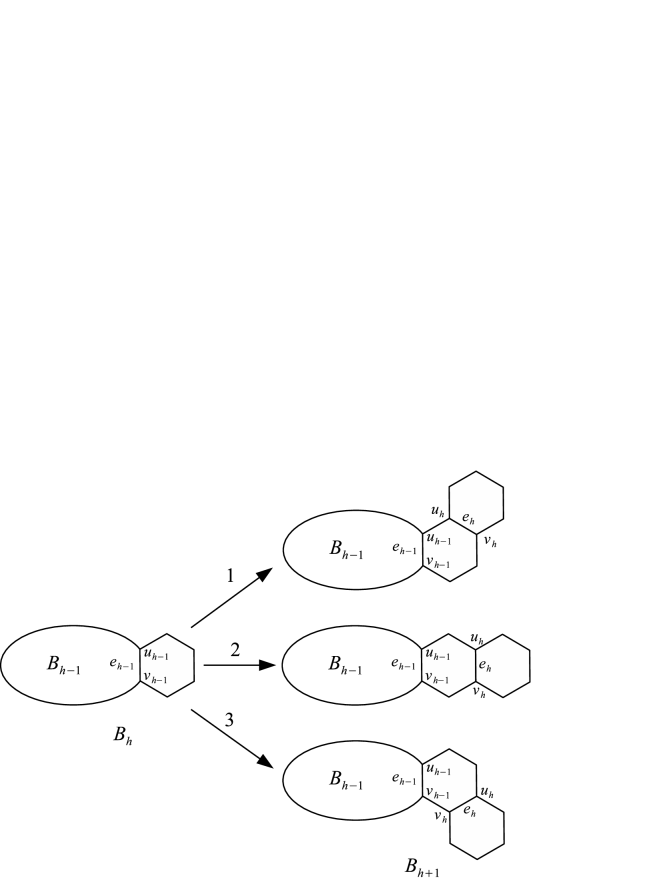
Figure 2: Three possible cases of annelating a $6$-cycle to a hexagonal chain.

For these three cases Theorem 3.2 implies:

Case 1:

$$H_{e}(B_{h},u_{h},x) = xH_{e}(B_{h-1},u_{h-1},x)+2+x+2x^{2}\,,$$

$$H_{e}(B_{h},v_{h},x) = x^{2}H_{e}(B_{h-1},u_{h-1},x)+2+2x+x^{2}\,,$$

$$H_{e}(B_{h},e_{h},x) = x^{2}H_{e}(B_{h-1},u_{h-1},x)+1+2x+x^{2}+x^{3}\,.$$

Case 2:

$$H_{e}(B_{h},u_{h},x) = x^{2}H_{e}(B_{h-1},u_{h-1},x)+2+2x+x^{2}\,,$$

$$H_{e}(B_{h},v_{h},x) = x^{2}H_{e}(B_{h-1},v_{h-1},x)+2+2x+x^{2}\,,$$

$$H_{e}(B_{h},e_{h},x) = x^{2}H_{e}(B_{h-1},e_{h-1},x)+1+2x+x^{2}+x^{3}\,.$$

Case 3:

$$H_{e}(B_{h},u_{h},x) = x^{2}H_{e}(B_{h-1},v_{h-1},x)+2+2x+x^{2}\,,$$

$$H_{e}(B_{h},v_{h},x) = xH_{e}(B_{h-1},v_{h-1},x)+2+x+2x^{2}\,,$$

$$H_{e}(B_{h},e_{h},x) = x^{2}H_{e}(B_{h-1},v_{h-1},x)+1+2x+x^{2}+x^{3}\,.$$

We write the above recurrences in a more concise form by setting $\alpha_{h}\equiv H_{e}(B_{h},x)$ , $\beta_{h}\equiv H_{e}(B_{h},u_{h},x)$ , $\gamma_{h}\equiv H_{e}(B_{h},v_{h},x)$ , and $\delta_{h}\equiv H_{e}(B_{h},e_{h},x)$. Then we obtain:

Theorem 4.1

Let $B_{h}$ be a benzenoid chain with $h$ hexagons. Then the edge-Hosoya polynomial $\alpha_{h}$ of $B_{h}$ satisfies the following recurrence

$$\alpha_{h}=\alpha_{h-1}+(x+x^{2})(\beta_{h-1}+\gamma_{h-1})+x^{2}\delta_{h-1}+5+4x+3x^{2}+3x^{3}\ ,$$

where $\alpha_{0}=\beta_{0}=\gamma_{0}=\delta_{0}=1$ . Moreover, $\beta_{h}$, $\gamma_{h}$ and $\delta_{h}$ obey the following recurrences, depending on the cases shown in Figure 2:

Case 1:

$$\beta_{h}=x\beta_{h-1}+2+x+2x^{2},\quad\gamma_{h}=x^{2}\beta_{h-1}+2+2x+x^{2},\quad\delta_{h}=x^{2}\beta_{h-1}+1+2x+x^{2}+x^{3}.$$

Case 2:

$$\beta_{h}=x^{2}\beta_{h-1}+2+2x+x^{2},\quad\gamma_{h}=x^{2}\gamma_{h-1}+2+2x+x^{2},\quad\delta_{h}=x^{2}\delta_{h-1}+1+2x+x^{2}+x^{3}.$$

Case 3:

$$\beta_{h}=x^{2}\gamma_{h-1}+2+2x+x^{2},\quad\gamma_{h}=x\gamma_{h-1}+2+x+2x^{2},\quad\delta_{h}=x^{2}\gamma_{h-1}+1+2x+x^{2}+x^{3}.$$

5 Closed formula for polyacenes

A hexagon $r$ of a benzenoid chain that is adjacent to two other hexagons (that is, an inner hexagon) contains two vertices of degree two. We say that $r$ is linearly connected if its two vertices of degree two are not adjacent. A benzenoid chain is called a linear benzenoid chain or a polyacene if every inner hexagon is linearly connected.

In this section we use Theorem 4.1 to obtain the closed formulas for the edge-Hosoya polynomial of polyacenes. Polyacene with $h$, $h\geq 1$, hexagons will be denoted by $L_{h}$, see Figure 3.

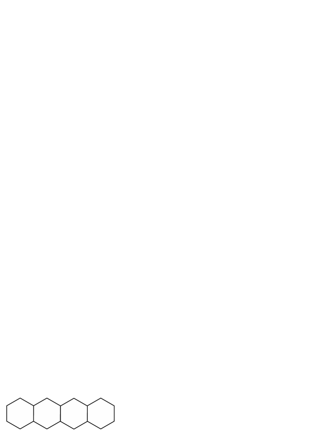
Figure 3: Linear benzenoid chain (polyacene) $L_{4}$.

One can notice that at every step of annelation we apply Case 2 of Theorem 4.1. The solutions of recursions for $\beta_{h},\gamma_{h}$, and $\delta_{h}$ are:

$$\beta_{h}=\gamma_{h}=\frac{x^{2h}(2x^{2}+2x+1)-x^{2}-2x-2}{x^{2}-1},$$

$$\delta_{h}=\frac{x^{2h}(x^{3}+2x^{2}+2x)--x^{3}-x^{2}-2x-1}{x^{2}-1}.$$

Finally, solving the recursion for $\alpha_{h}$ we obtain the edge-Hosoya polynomial of $L_{h}$:

$$H_{e}(L_{h},x) = \frac{x^{2h+5}+6x^{2h+4}+10x^{2h+3}+6x^{2h+2}+2x^{2h+1}}{(x^{2}-1)^{2}}$$

$$+ \frac{2hx^{7}-(9h+1)x^{5}-(7h+5)x^{4}-(h+10)x^{3}+2(h-4)x^{2}+2(4h-1)x+5h+1}{(x^{2}-1)^{2}}.$$

By the obtained result and Equations (1),(2) it is possible to compute the closed formulas for the edge-Wiener index and the edge-hyper-Wiener index of polyacenes. However, these formulas were found in [11, 9] and corrected in [15].

References

• [1] A. Behmaram, H. Yousefi-Azari, A. R. Ashrafi, Some new results on distance-based polynomials, MATCH Commun. Math. Comput. Chem. 65 (2011) 39–50.
• [2] G. G. Cash, Relationship between the Hosoya polynomial and the hyper-Wiener index, Appl. Math. Lett. 15 (2002) 893–895.
• [3] A. Chen, X. Xiong, F. Lin, Explicit relation between the Wiener index and the edge-Wiener index of the catacondensed hexagonal systems, Appl. Math. Comput. 273 (2016) 1100–1106.
• [4] M. Črepnjak, N.Β Tratnik, The edge-Wiener index, the Szeged indices and the PI index of benzenoid systems in sub-linear time, MATCH Commun. Math. Comput. Chem. 78 (2017) 675–688.
• [5] E. Deutsch, S. KlavΕΎar, Computing the Hosoya polynomial of graphs from primary subgraphs, MATCH Commun. Math. Comput. Chem. 70 (2013) 627–644.
• [6] I. Gutman, S. KlavΕΎar, M. PetkovΕ‘ek, P. Ε½igert, On Hosoya polynomials of benzenoid graphs, MATCH Commun. Math. Comput. Chem. 43 (2001) 49–66.
• [7] H. Hosoya, On some counting polynomials in chemistry, Discrete Appl. Math. 19 (1988) 239–257.
• [8] A. Iranmanesh, I. Gutman, O. Khormali, A. Mahmiani, The edge versions of Wiener index, MATCH Commun. Math. Comput. Chem. 61 (2009) 663–672.
• [9] A. Iranmanesh, A. Soltani Kafrani, O. Khormali, A new version of hyper-Wiener index, MATCH Commun. Math. Comput. Chem. 65 (2011) 113–122.
• [10] A. Kelenc, S. KlavΕΎar, N. Tratnik, The edge-Wiener index of benzenoid systems in linear time, MATCH Commun. Math. Comput. Chem. 74 (2015) 521–532.
• [11] O. Khormali, A. Iranmanesh, I. Gutman, A. Ahmadi, Generalized Schultz index and its edge versions, MATCH Commun. Math. Comput. Chem. 64 (2010) 783–798.
• [12] S. KlavΕΎar, M. Mollard, Wiener index and Hosoya polynomial of Fibonacci and Lucas cubes, MATCH Commun. Math. Comput. Chem. 68 (2012) 311–324.
• [13] M. Knor, R. Ε krekovski, A. Tepeh, An inequality between the edge-Wiener index and the Wiener index of a graph, Appl. Math. Comput. 269 (2015) 714–721.
• [14] X. Lin, S. Xu, J. Yeh, Hosoya polynomials of circumcoronene series, MATCH Commun. Math. Comput. Chem. 69 (2013) 755–763.
• [15] N. Tratnik, A method for computing the edge-hyper-Wiener index of partial cubes and an algorithm for benzenoid systems, Appl. Anal. Discr. Math., to appear.
• [16] N. Tratnik, P. Ε½igert PleterΕ‘ek, Relationship between the Hosoya polynomial and the edge-Hosoya polynomial of trees, MATCH Commun. Math. Comput. Chem. 78 (2017) 181–187.
• [17] S. Xu, H. Zhang, Hosoya polynomials under gated amalgamations, Discrete Appl. Math. 156 (2008) 2407–2419.
• [18] S. Xu, H. Zhang, M. V. Diudea, Hosoya polynomials of zig-zag open-ended nanotubes, MATCH Commun. Math. Comput. Chem. 57 (2007) 443–456.