Two-stage fourth-order accurate time discretizations for 1D and 2D special relativistic hydrodynamics

Abstract

This paper studies the two-stage fourth-order accurate time discretization [J.Q. Li and Z.F. Du, SIAM J. Sci. Comput., 38(2016)] and its application to the special relativistic hydrodynamical equations. Our analysis reveals that the new two-stage fourth-order accurate time discretizations can be proposed. With the aid of the direct Eulerian GRP (generalized Riemann problem) methods and the analytical resolution of the local “quasi 1D” GRP, the two-stage fourth-order accurate time discretizations are successfully implemented for the 1D and 2D special relativistic hydrodynamical equations. Several numerical experiments demonstrate the performance and accuracy as well as robustness of our schemes.

Keywords: Time discretization, shock-capturing scheme, GRP method, relativistic hydro-dynamics, hyperbolic conservation laws.

1 Introduction

The relativistic hydrodynamics (RHD) plays the leading role in astrophysics and nuclear physics etc. The RHDs is necessary in situations where the local velocity of the flow is close to the light speed in vacuum, or where the local internal energy density is comparable (or larger) than the local rest mass density of fluid. The paper is concerned with developing higher-order accurate numerical schemes for the 1D and 2D special RHDs. The $d$-dimensional governing equations of the special RHDs is a first-order quasilinear hyperbolic system. In the laboratory frame, it can be written into the divergence form

$$\frac{\partial\mbox{\boldmath\small$U$}}{\partial\mbox{\boldmath\small$t$}}+\sum_{i=1}^{d}\frac{\partial\mbox{\boldmath\small$F$}_{i}(\mbox{\boldmath\small$U$})}{\partial x_{i}}=0,$$ (1)

where $d=1$ or 2, and $U$ and $\mbox{\boldmath\small$F$}_{i}(\mbox{\boldmath\small$U$})$ denote the conservative vector and the flux in the $x_{i}$-direction, respectively, defined by

$$\mbox{\boldmath\small$U$}=(D,\mbox{\boldmath\small$m$},E)^{T},\ \mbox{\boldmath\small$F$}_{i}(\mbox{\boldmath\small$U$})=(Dv_{i},v_{i}\mbox{\boldmath\small$m$}+p\mbox{\boldmath\small$e$}_{i},m_{i})^{T},i=1,\cdots,d,$$ (2)

with the mass density $D=\rho W$, the momentum density (row) vector $\mbox{\boldmath\small$m$}=DhW\mbox{\boldmath\small$v$}$, the energy density $E=DhW-p$, and the row vector $\mbox{\boldmath\small$e$}_{i}$ denoting the $i$-th row of the unit matrix of size 2. Here $\rho$ is the rest-mass density, $v_{i}$ denotes the fluid velocity in the $x_{i}$-direction, $p$ is the gas pressure, $W=1/\sqrt{1-v^{2}}$ is the Lorentz factor with $v:=\left(v_{1}^{2}+\cdots+v_{d}^{2}\right)^{1/2}$, $h$ is the specific enthalpy defined by

$$h=1+e+\frac{p}{\rho},$$

with units in which the speed of light $c$ is equal to one, and $e$ is the specific internal energy. Throughout the paper, the equation of state (EOS) will be restricted to the $\Gamma$-law

$$p=(\Gamma-1)\rho e,$$ (3)

where the adiabatic index $\Gamma\in(1,2]$. The restriction of $\Gamma\leq 2$ is required for the compressibility assumptions and the causality in the theory of relativity (the sound speed does not exceed the speed of light $c=1$).

The RHD equations (1) are highly nonlinear so that their analytical treatment is extremely difficult. Numerical computation has become a major way in studying RHDs. The pioneering numerical work can date back to the Lagrangian finite difference code via artificial viscosity for the spherically symmetric general RHD equations [19, 20]. Multi-dimensional RHD equations were first solved in [26] by using the Eulerian finite difference method with the artificial viscosity technique. Later, modern shock-capturing methods were extended to the RHD (including RMHD) equations. Some representative methods are the HLL (Harten-Lax-van Leer) scheme [6], HLLC (HLLC contact) schemes [21, 12], Riemann solver [2], approximate Riemann solvers based on the local linearization [16, 15], second-order GRP (generalized Riemann problem) schemes [37, 38, 30], third-order GRP scheme [36], locally evolution Galerkin method [29], discontinuous Galerkin (DG) methods [39, 40], gas-kinetic schemes (GKS) [23, 4], adaptive mesh refinement methods [1, 13], and moving mesh methods [10, 11] etc. Recently, the higher-order accurate physical-constraints-preserving (PCP) WENO (weighted essentially non-oscillatory) and DG schemes were developed for the special RHD equations [31, 33, 24]. They were built on studying the admissible state set of the special RHDs. The admissible state set and PCP schemes of the special ideal RMHDs were also studied for the first time in [32], where the importance of divergence-free fields was revealed in achieving PCP methods. Those works were successfully extended to the special RHDs with a general equation of state [34, 33] and the general RHDs [28].

In comparison with second-order shock-capturing schemes, the higher-order methods can provide more accurate solutions, but they are less robust and more complicated. For most of the existing higher-order methods, the Runge-Kutta time discretization is usually used to achieve higher order temporal accuracy. For example, a four-stage fourth-order Runge-Kutta method (see e.g. [40]) is used to achieve a fourth-order time accuracy. If each stage of the time discretization needs to call the Riemann solver or the resolution of the local GRP, then the shock-capturing scheme with multi-stage time discretization for (1) is very time-consuming. Recently, based on the time-dependent flux function of the GRP, a two-stage fourth-order accurate time discretization was developed for Lax-Wendroff (LW) type flow solvers, particularly applied for the hyperbolic conservation laws [18]. Such two-stage LW time stepping method does also provide an alternative framework for the development of a fourth-order GKS with a second-order flux function [22].

The aim of this paper is to study the two-stage fourth-order accurate time discretization [18] and its application to the special RHD equations (1). Based our analysis, the new two-stage fourth-order accurate time discretizations can be proposed. With the aid of the direct Eulerian GRP methods and the analytical resolution of the local “quasi 1D” GRP, those two-stage fourth-order accurate time discretizations can be conveniently implemented for the special RHD equations. Their performance and accuracy as well as robustness can be demonstrated by numerical experiments. The paper is organized as follows. Section 2 studies the two-stage fourth-order accurate time discretizations and applies them to the special RHD equations. Section 3 conducts several numerical experiments to demonstrate the accuracy and efficiency of the proposed methods. Conclusions are given in Section 4.

2 Numerical methods

In this section, we study the two-stage fourth-order accurate time discretization [18] and then propose the new two-stage fourth-order accurate time discretizations. With the aid of the direct Eulerian GRP methods, those two-stage time discretizations can be implemented for the special RHD equations (1).

2.1 Two-stage fourth-order time discretizations

Consider the time-dependent differential equation

$$u_{t}=L(u),\ t>0,$$ (4)

which can be a semi-discrete scheme for the conservation laws (1).

Assume that the solution $u$ of (4) is a fully smooth function of $t$ and $L(u)$ is also fully smooth, and give a partition of the time interval by $t_{n}=n\tau$, where $\tau$ denotes the time stepsize and $n\in\mathbb{Z}$. The Taylor series expansion of $u$ in $t$ reads

$$u^{n+1}= \Big{(}u+\tau u_{t}+\frac{\tau^{2}}{2!}u_{tt}+\frac{\tau^{3}}{3!}u_{ttt}+\frac{\tau^{4}}{4!}u_{tttt}\Big{)}^{n}+{\mathcal{O}}(\tau^{5})$$

$$= \Big{(}u+\tau u_{t}+\frac{\tau^{2}}{6}u_{tt}\Big{)}^{n}+{2}\frac{\tau^{2}}{6}\Big{(}\big{(}u+\frac{\tau}{2}u_{t}+\frac{\tau^{2}}{8}u_{tt}\big{)}_{tt}\Big{)}^{n}+{\mathcal{O}}(\tau^{5}).$$ (5)

Substituting (4) into (5) gives

$$u^{n+1}= \Big{(}u+\tau L(u)+\frac{\tau^{2}}{6}\partial_{t}L(u)\Big{)}^{n}+{2}\frac{\tau^{2}}{6}\Big{(}\big{(}u+\frac{\tau}{2}L(u)+\frac{\tau^{2}}{8}\partial_{t}L(u)\big{)}_{tt}\Big{)}^{n}+{\mathcal{O}}(\tau^{5})$$

$$= \Big{(}u+\tau L(u)+\frac{\tau^{2}}{6}\partial_{t}L(u)\Big{)}^{n}+{2}\frac{\tau^{2}}{6}\left((u^{*})_{tt}\right)^{n}+{\mathcal{O}}(\tau^{5}),$$ (6)

where

$$u^{*}:=u+\frac{1}{2}\tau L(u)+\frac{1}{8}\tau^{2}L_{t}(u)=u\left(t_{n}+\frac{\tau}{2}\right)+{\mathcal{O}}(\tau^{3}).$$

Because

$$u^{*}_{t}= u_{t}+\frac{1}{2}\tau L_{t}(u)+\frac{1}{8}\tau^{2}L_{tt}(u)=L(u)+\frac{1}{2}\tau L_{u}L(u)+\frac{1}{8}\tau^{2}\left((L_{u})^{2}L+L_{uu}L^{2}\right),$$

$$L(u^{*})= L(u)+L_{u}\left(\frac{1}{2}\tau L(u)+\frac{1}{8}\tau^{2}L_{t}(u)\right)+\frac{1}{2}L_{uu}\left(\frac{1}{2}\tau L(u)+\frac{1}{8}\tau^{2}L_{t}(u)\right)^{2}{+\cdots},$$

one has

$$u^{*}_{t}=L(u^{*})+{\mathcal{O}}(\tau^{3}),\ u^{*}_{tt}=L_{t}(u^{*})+{\mathcal{O}}(\tau^{3}).$$

Combining the second equation with (6) gives

$$u^{n+1}= \Big{(}u+\tau L(u)+\frac{\tau^{2}}{6}\partial_{t}L(u)\Big{)}^{n}+{2}\frac{\tau^{2}}{6}\left(L_{t}(u^{*})\right)^{n}+{\mathcal{O}}(\tau^{5}).$$

The above discussion gives the two-stage fourth-order accurate time discretization of (4) [18]:

• Compute the intermediate value

  $$u^{*}=u^{n}+\frac{1}{2}\tau L(u^{n})+\frac{1}{8}\tau^{2}\frac{\partial}{\partial t}L(u^{n}),$$ (7)

• Evolve the solution at $t_{n+1}$ via

  $$u^{n+1}=u^{n}+\tau L(u^{n})+\frac{1}{6}\tau^{2}\left(\frac{\partial}{\partial t}L(u^{n})+{2}\frac{\partial}{\partial t}L(u^{*})\right).$$ (8)

Obviously, the additive decomposition in (5) is not unique. For example, it can be replaced with a more general decomposition

$$u^{n+1}= \Big{(}u+\tau L(u)+\frac{{\alpha}\tau^{2}}{2}\partial_{t}L(u)\Big{)}^{n}+{}\frac{(1-\alpha)\tau^{2}}{2}\Big{(}\big{(}\tilde{u}^{*}\big{)}_{tt}\Big{)}^{n}+{O(\tau^{5})},$$ (9)

with $\alpha\neq 1$ and

$$\tilde{u}^{*}:=u+\frac{\tau}{3(1-\alpha)}L(u)+\frac{\tau^{2}}{12(1-\alpha)}\partial_{t}L(u).$$ (10)

If $\alpha=\frac{1}{3}$, then (9) becomes the additive decomposition in (5) for the two-stage fourth-order time discretization [18].

The identity (10) implies

$$\tilde{u}^{*}_{t}= L(u)+\frac{\tau}{3(1-\alpha)}L_{t}(u)+\frac{\tau^{2}}{12(1-\alpha)}\partial_{tt}L(u).$$ (11)

Comparing (11) to the following Taylor series expansion

$$L(\tilde{u}^{*})= L(u)+L_{u}\left(\frac{\tau}{3(1-\alpha)}L+\frac{\tau^{2}}{12(1-\alpha)}L_{t}(u)\right)+\frac{1}{2}L_{uu}\left(\frac{\tau}{3(1-\alpha)}L+\frac{\tau^{2}}{12(1-\alpha)}L_{t}(u)\right)^{2}{+\cdots},$$

gives

$$\tilde{u}^{*}_{t}=L(\tilde{u}^{*})+\frac{\tau^{2}}{12(1-\alpha)}\left(1-\frac{2}{3(1-\alpha)}\right)L_{uu}(u_{t})^{2}+{\mathcal{O}}(\tau^{3}).$$

If

$$1-\frac{2}{3(1-\alpha)}=C\tau^{p},\ p\geq 1,$$ (12)

where $C$ is independent on $\tau$, then

$$\tilde{u}^{*}_{t}=L(\tilde{u}^{*})+{\mathcal{O}}(\tau^{3}).$$

Therefore, if $\alpha=\alpha(\hat{\tau})$ is a differentiable function of $\hat{\tau}$ and satisfies $\alpha(0)=1/3$, $\alpha\neq 1$, and $\hat{\tau}=C\tau^{p}$, then (12) does hold. For example, we may choose $\alpha=(1-6\hat{\tau})/(3-6\hat{\tau})$ with $\hat{\tau}\neq 1/2$. At this time, one has

$$\tilde{u}^{*}=u\left(t+\frac{\tau}{3(1-\alpha)}\right)+{\mathcal{O}}(\tau^{3}),$$

and similarly, from (10) and the Taylor series expansion of $L_{t}\left(\tilde{u}^{*}\right)$ at $u$, one can get

$$\tilde{u}^{*}_{tt}=L_{t}\left(\tilde{u}^{*}\right)+{\mathcal{O}}(\tau^{3}).$$ (13)

Substituting (13) into (9) gives

$$u^{n+1}= \Big{(}u+\tau L(u)+\frac{{\alpha}\tau^{2}}{2}\partial_{t}L(u)\Big{)}^{n}+\frac{{(1-\alpha)}\tau^{2}}{2}\Big{(}\partial_{t}L(\tilde{u}^{*})\Big{)}^{n}+{\mathcal{O}}(\tau^{5}).$$

In conclusion, when $\alpha=\alpha(\hat{\tau})$ is a differentiable function of $\hat{\tau}=C\tau^{p}$ and satisfies $\alpha(0)=1/3$ and $\alpha\neq 1$, where $p\geq 1$ and $C$ is independent on $\tau$, the additive decomposition (9) can give new two-stage fourth-order accurate time discretizations as follows:

• Compute the intermediate value

  $$u^{*}=u^{n}+\frac{1}{3(1-\alpha)}\tau L(u^{n})+\frac{\tau^{2}}{12(1-\alpha)}\frac{\partial}{\partial t}L(u^{n}),$$ (14)

• Evolve the solution at $t_{n+1}$ via

  $$u^{n+1}=u^{n}+\tau L(u^{n})+\frac{\alpha\tau^{2}}{2}\frac{\partial}{\partial t}L(u^{n})+\frac{(1-\alpha)\tau^{2}}{2}\frac{\partial}{\partial t}L(u^{*}).$$ (15)

2.2 Application of two-stage time discretizations to 1D RHD equations

In this section, we apply the above two-stage fourth-order time discretizations to the 1D RHD equations, i.e. (1) with $d=1$. For the sake of convenience, the symbols $x_{1}$ and $v_{1}$ are replaced with $x$ and $u$, respectively, and a uniform partition of the spatial domain is given by $I_{j}=(x_{j-\frac{1}{2}},\,x_{j+\frac{1}{2}})$ with $\Delta x=x_{j+\frac{1}{2}}-x_{j-\frac{1}{2}}$.

For the given “initial” approximate cell averages $\{\overline{\mbox{\boldmath\small$U$}}^{n}_{j}\}$ at $t_{n}$, we want to reconstruct the WENO values of $U$ and $\partial_{x}\mbox{\boldmath\small$U$}$ at the cell boundaries, denoted by $\mbox{\boldmath\small$U$}^{\pm,n}_{j+\frac{1}{2}}$ and $(\partial_{x}\mbox{\boldmath\small$U$})^{\pm,n}_{j+\frac{1}{2}}$. Our initial reconstruction procedure is given as follows:

(1)

Use the standard 5th-order WENO reconstruction [14] to get $\mbox{\boldmath\small$U$}^{\pm,n}_{j+\frac{1}{2}}$ with the aid of the characteristic decomposition. If $\mbox{\boldmath\small$U$}^{\pm,n}_{j+\frac{1}{2}}$ does not belong to the admissible state set of 1D RHD equations [31], then we set $\mbox{\boldmath\small$U$}^{\pm,n}_{j+\frac{1}{2}}=\overline{\mbox{\boldmath\small$U$}}_{j}^{n}$ directly in order to avoid the nonphysical solution as soon as possible.

(2)

Calculate $(\overline{\partial_{x}\mbox{\boldmath\small$U$}})_{j}^{n}=\frac{1}{\Delta x}(\mbox{\boldmath\small$U$}^{-,n}_{j+\frac{1}{2}}-\mbox{\boldmath\small$U$}^{+,n}_{j-\frac{1}{2}})$, which is the approximate cell average value of $\partial_{x}\mbox{\boldmath\small$U$}$ over the cell $I_{j}$, and then use the above WENO again to get $(\partial_{x}\mbox{\boldmath\small$U$})^{\pm,n}_{j+\frac{1}{2}}$.

Such initial reconstruction is also used at $t_{*}=t_{n}+\tau/(3-3\alpha)$, where $\alpha=\alpha(\hat{\tau})$ is a differentiable function of $\hat{\tau}$ and satisfies $\alpha(0)=1/3$, $\alpha\neq 1$, and $\hat{\tau}=C\tau^{p}$ with $p\geq 1$ and $C$ independent on $\tau$.

The two-stage fourth-order time discretizations in Section 2.1 can be applied to the 1D RHD equations by the following steps.

• For the reconstructed data $\mbox{\boldmath\small$U$}^{\pm,n}_{j+\frac{1}{2}}$ and $(\partial_{x}\mbox{\boldmath\small$U$})^{\pm,n}_{j+\frac{1}{2}}$, following the GRP method [37], solve the Riemann problem of

  $$\mbox{\boldmath\small$U$}_{t}+\mbox{\boldmath\small$F$}_{1}(\mbox{\boldmath\small$U$})_{x}=0,\ t>t_{n},\\$$ (16)

  to get $\mbox{\boldmath\small$U$}_{j+\frac{1}{2}}^{RP,n}$ and then resolve analytically the GRP of (16) to obtain the value of $(\partial\mbox{\boldmath\small$U$}/\partial t)_{j+\frac{1}{2}}^{n}$.

• Compute the intermediate values $\{\overline{\mbox{\boldmath\small$U$}}_{j}^{*}\}$ by

  $$\overline{\mbox{\boldmath\small$U$}}_{j}^{*}=\overline{\mbox{\boldmath\small$U$}}^{n}_{j}+\frac{\tau}{3(1-\alpha)}L_{j}(\overline{\mbox{\boldmath\small$U$}}^{n})+\frac{\tau^{2}}{12(1-\alpha)}\partial_{t}L_{j}(\overline{\mbox{\boldmath\small$U$}}^{n}),$$ (17)

  where the terms $L_{j}(\overline{\mbox{\boldmath\small$U$}}^{n})$ and $\partial_{t}L_{j}(\overline{\mbox{\boldmath\small$U$}}^{n})$ are given by

  $$L_{j}(\overline{\mbox{\boldmath\small$U$}}^{n})=-\frac{1}{\Delta x}\left(\mbox{\boldmath\small$F$}_{1}(\mbox{\boldmath\small$U$}_{j+\frac{1}{2}}^{RP,n})-\mbox{\boldmath\small$F$}_{1}(\mbox{\boldmath\small$U$}_{j-\frac{1}{2}}^{RP,n})\right),$$ (18)

  and

  $$\partial_{t}L_{j}(\overline{\mbox{\boldmath\small$U$}}^{n})=-\frac{1}{\Delta x}\left((\partial_{t}\mbox{\boldmath\small$F$}_{1})_{j+\frac{1}{2}}^{n}-(\partial_{t}\mbox{\boldmath\small$F$}_{1})_{j-\frac{1}{2}}^{n}\right),$$ (19)

  with

  $$(\partial_{t}\mbox{\boldmath\small$F$}_{1})_{j\pm\frac{1}{2}}^{n}=\frac{\partial\mbox{\boldmath\small$F$}_{1}}{\partial\mbox{\boldmath\small$U$}}\left(\mbox{\boldmath\small$U$}_{j\pm\frac{1}{2}}^{RP,n}\right)\cdot\left(\frac{\partial\mbox{\boldmath\small$U$}}{\partial t}\right)_{j\pm\frac{1}{2}}^{n}.$$

• Reconstruct the values $\mbox{\boldmath\small$U$}^{\pm,*}_{j+\frac{1}{2}}$ and $(\partial_{x}\mbox{\boldmath\small$U$})^{\pm,*}_{j+\frac{1}{2}}$ with $\{\overline{\mbox{\boldmath\small$U$}}_{j}^{*}\}$ by the above initial reconstruction procedure, and then resolve analytically the local GRP of (16) to get $\mbox{\boldmath\small$U$}_{j+\frac{1}{2}}^{RP,*}$ and $(\partial\mbox{\boldmath\small$U$}/\partial t)_{j+\frac{1}{2}}^{*}$.

• Evolve the solution at $t_{n+1}=t_{n}+\tau$ by

  $$\overline{\mbox{\boldmath\small$U$}}_{j}^{n+1}=\overline{\mbox{\boldmath\small$U$}}_{j}^{n}+\tau L_{j}(\overline{\mbox{\boldmath\small$U$}}^{n})+\frac{\alpha\tau^{2}}{2}\partial_{t}L_{j}(\overline{\mbox{\boldmath\small$U$}}^{n})+\frac{(1-\alpha)\tau^{2}}{2}\partial_{t}L_{j}(\overline{\mbox{\boldmath\small$U$}}^{*}),$$ (20)

  where

  $$\partial_{t}L_{j}(\overline{\mbox{\boldmath\small$U$}}^{*})=-\frac{1}{\Delta x}\left((\partial_{t}\mbox{\boldmath\small$F$}_{1})_{j+\frac{1}{2}}^{*}-(\partial_{t}\mbox{\boldmath\small$F$}_{1})_{j-\frac{1}{2}}^{*}\right),$$ (21)

  with

  $$(\partial_{t}\mbox{\boldmath\small$F$}_{1})_{j\pm\frac{1}{2}}^{*}=\frac{\partial\mbox{\boldmath\small$F$}_{1}}{\partial\mbox{\boldmath\small$U$}}\left(\mbox{\boldmath\small$U$}_{j\pm\frac{1}{2}}^{RP,*}\right)\cdot\left(\frac{\partial\mbox{\boldmath\small$U$}}{\partial t}\right)_{j\pm\frac{1}{2}}^{*}.$$

2.3 Application of two-stage time discretizations to 2D RHD equations

In this section, we apply the two-stage fourth-order time discretizations to the 2D RHD equations, i.e. (1) with $d=2$ with the aid of the analytical resolution of the local “quasi 1D” GRP and an adaptive primitive-conservative scheme. The latter given in [17] is used to reduce the spurious solution generated by the conservative scheme across the contact discontinuity, see Example 2.1. Similarly, the symbols $(x_{1},x_{2})$ and $(v_{1},v_{2})$ are replaced with $(x,y)$ and $(u,v)$, respectively, and a uniform partition of the spatial domain is given by $I_{jk}{=}(x_{j-\frac{1}{2}},\,x_{j+\frac{1}{2}})\times(y_{k-\frac{1}{2}},\,y_{k+\frac{1}{2}})$ with $\Delta x=x_{j+\frac{1}{2}}-x_{j-\frac{1}{2}}$ and $\Delta y=y_{k+\frac{1}{2}}-y_{k-\frac{1}{2}}$.

Example 2.1

Because of the nonlinearity of (1), when a conservative scheme is used, a spurious solution across the contact discontinuity, a well-known phenomenon in multi-fluid systems, can arise even for a single material. It is similar to the phenomenon mentioned in [17]. To clarify that, let us solve the Riemann problem of (1) with the initial data

$$(\rho,u,v,p)(x,y,0)\;=\;\begin{cases}(0.5,-0.5,0.5,5),&x>0.5,\\ (0.5,-0.5,-0.5,5),&x<0.5.\end{cases}$$ (22)

The computational domain is taken as $[0,1]\times[0,1]$. Fig. 1 gives the solutions obtained by using the 2D (first-order, conservative) Godunov method. Fig. 2 gives the solutions obtained by using the 2D two-stage fourth-order conservative method. The obvious oscillations near the contact discontinuity are observed, in other words, the spurious solutions have been generated near the contact discontinuity. It is easy to verify it theoretically. To overcome such difficulty, the generalized Osher-type scheme in an adaptive primitive-conservative framework [17] can be employed to avoid or reduce the above spurious solutions at the expense of the conservation. Figs. 3 and 4 do respectively display more better solutions obtained by the adaptive primitive-conservative scheme with the reconstructions of the characteristic and primitive variables than those in Figs. 1 and 2, in which the generalized Osher-type scheme is adaptively used to solve the RHD equations (1) in the equivalently primitive form

$$\partial_{t}\mbox{\boldmath\small$V$}+\widetilde{\mbox{\boldmath\small$A$}}(\mbox{\boldmath\small$V$})\partial_{x}\mbox{\boldmath\small$V$}+\widetilde{\mbox{\boldmath\small$B$}}(\mbox{\boldmath\small$V$})\partial_{y}\mbox{\boldmath\small$V$}=0,$$ (23)

where $\mbox{\boldmath\small$V$}=(\rho,\,u,\,v,\,p)^{T}$ and

$$\widetilde{\mbox{\boldmath\small$A$}}(\mbox{\boldmath\small$V$})=u\cdot\mbox{\boldmath\small$I$}_{4}+\begin{pmatrix}0&\dfrac{\rho}{1-(u^{2}+v^{2})c_{s}^{2}}&0&\dfrac{-u}{W^{2}h[1-(u^{2}+v^{2})c_{s}^{2}]}\\ 0&\dfrac{-uc_{s}^{2}}{W^{2}[1-(u^{2}+v^{2})c_{s}^{2}]}&0&\dfrac{H}{\rho hW^{2}[1-(u^{2}+v^{2})c_{s}^{2}]}\\ 0&\dfrac{-vc_{s}^{2}}{W^{2}[1-(u^{2}+v^{2})c_{s}^{2}]}&0&\dfrac{-uv(1-c_{s}^{2})}{\rho hW^{2}[1-(u^{2}+v^{2})c_{s}^{2}]}\\ 0&\dfrac{\rho hc_{s}^{2}}{1-(u^{2}+v^{2})c_{s}^{2}}&0&\dfrac{-uc_{s}^{2}}{W^{2}[1-(u^{2}+v^{2})c_{s}^{2}]}\end{pmatrix},$$ (24)

with $H=1-u^{2}-v^{2}c_{s}^{2}$ and $c_{s}^{2}=\frac{\Gamma p}{\rho h}$. The matrix $\widetilde{\mbox{\boldmath\small$B$}}(\mbox{\boldmath\small$V$})$ can be gotten by exchanging $u$ and $v$, and then the second and third row, and the second and third column of the matrix $\widetilde{\mbox{\boldmath\small$A$}}$.

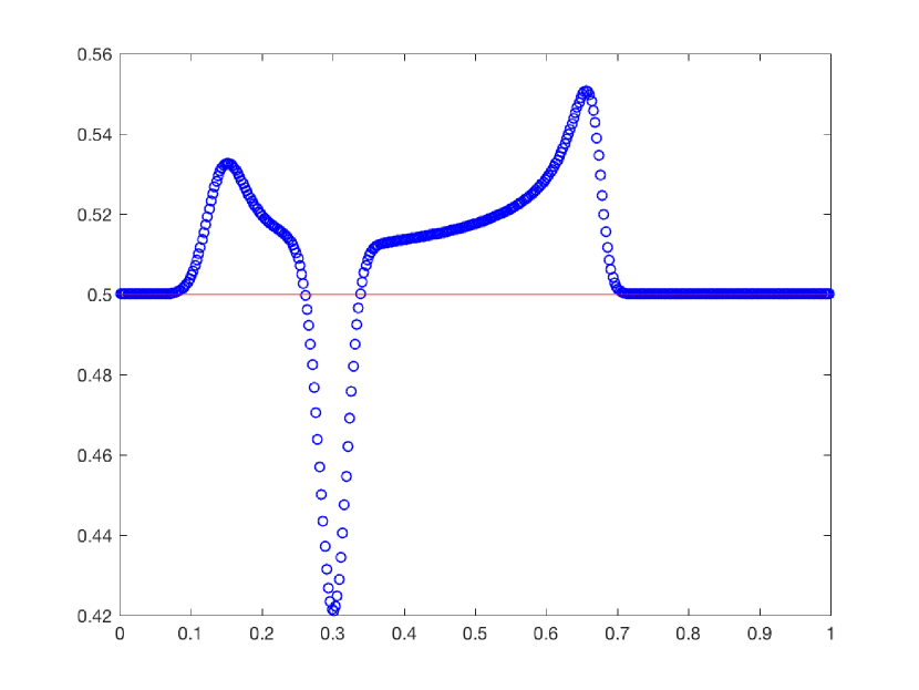
(a) $\rho$

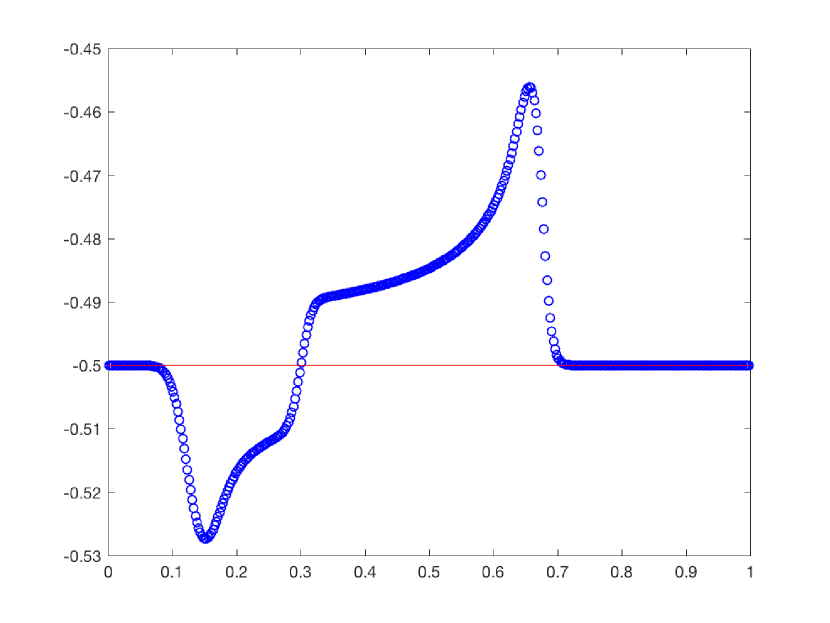
(b) $u$

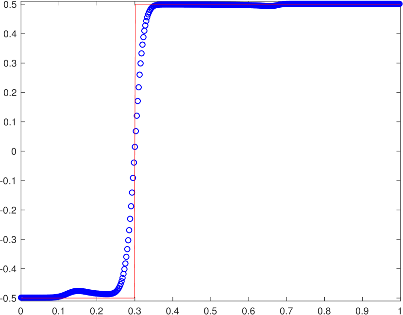
(c) $v$

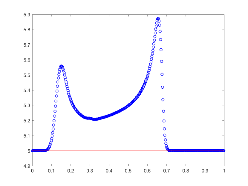
(d) $p$

Figure 1: Example 2.1: The solutions at $t=0.4$ obtained by the first-order Godunov method along the line $y=0.5$ with $400\times 40$ uniform cells.

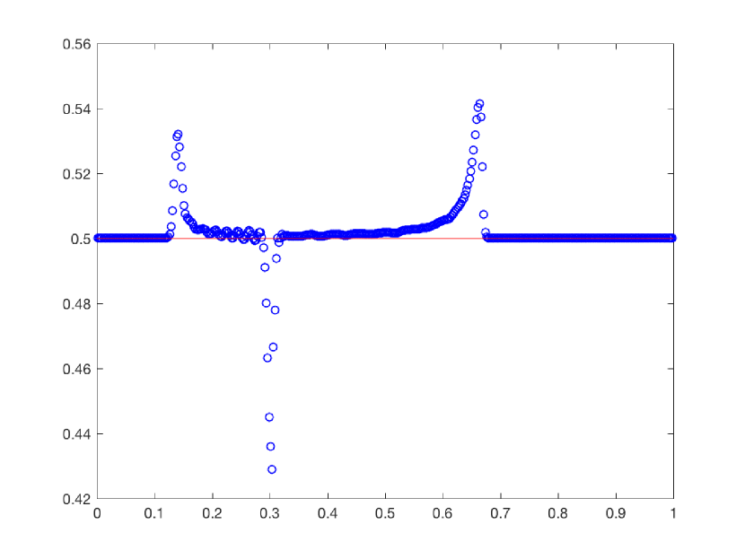
(a) $\rho$

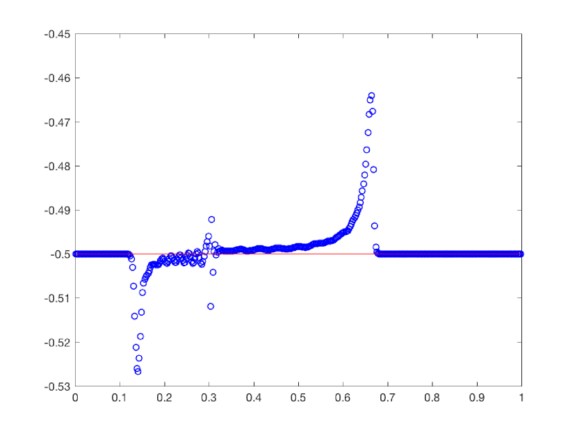
(b) $u$

(c) $v$

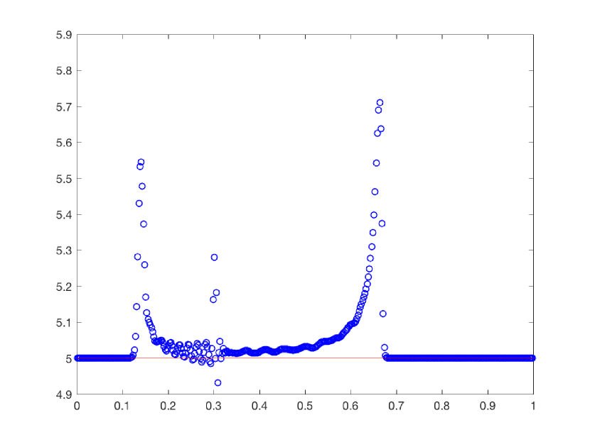
(d) $p$

Figure 2: Same as Fig. 1 except for two-stage fourth-order conservative scheme with the reconstructed characteristic variables.

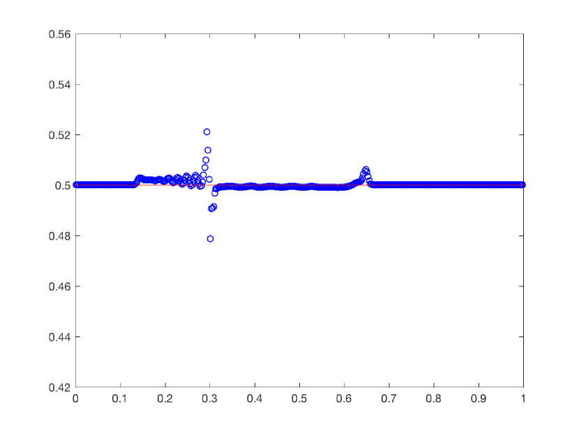
(a) $\rho$

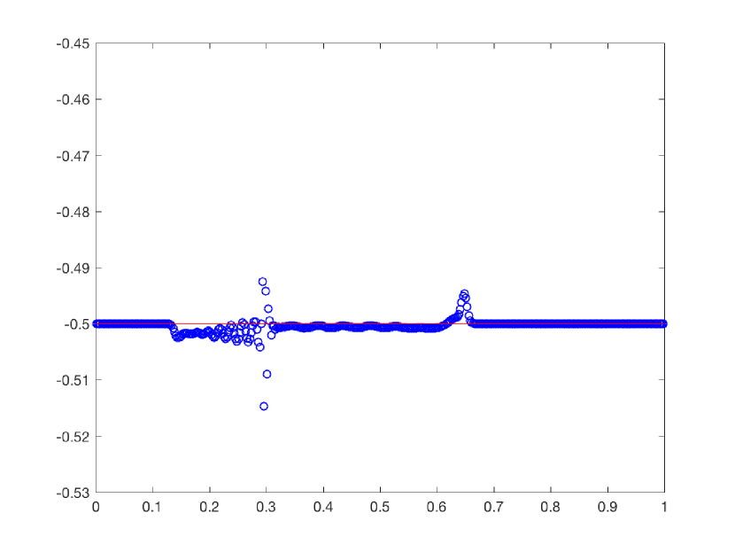
(b) $u$

(c) $v$

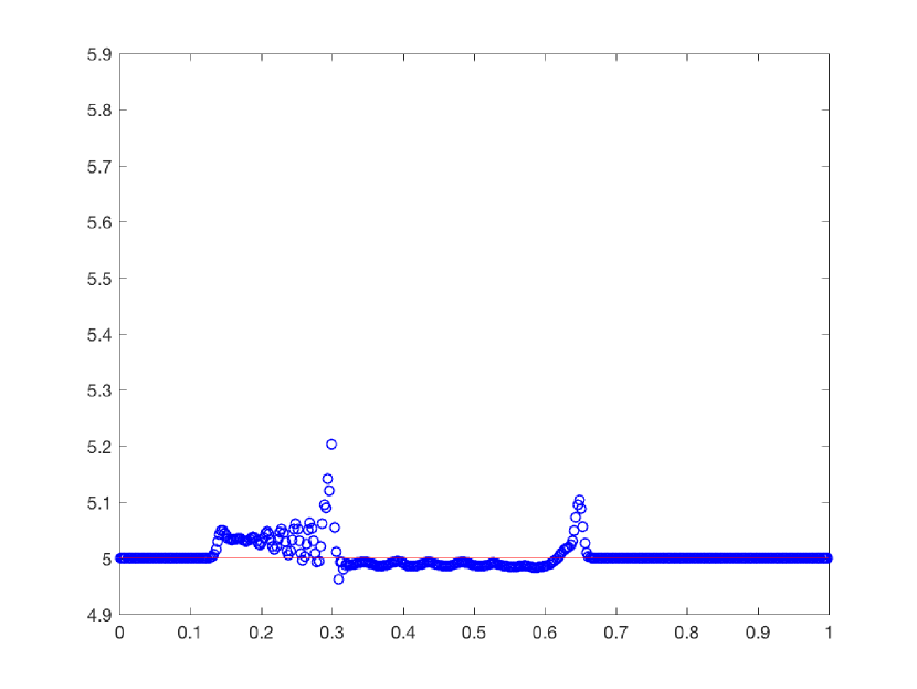
(d) $p$

Figure 3: Same as Fig. 1 except for two-stage fourth-order adaptive primitive-conservative scheme with the reconstructed characteristic variables.

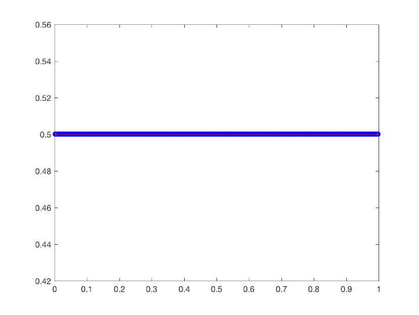
(a) $\rho$

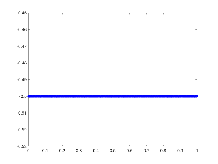
(b) $u$

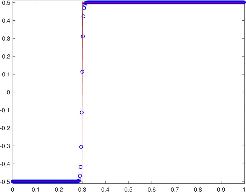
(c) $v$

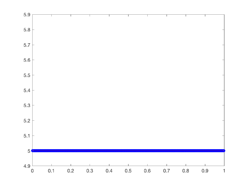
(d) $p$

Figure 4: Same as Fig. 3 except for the reconstructed primitive variables.

With the given “initial” cell-average data $\{{\overline{\mbox{\boldmath\small$U$}}}^{n}_{jk}\}$, in the $x-$direction, we want to reconstruct $\mbox{\boldmath\small$U$}^{\pm,n}_{j+\frac{1}{2},k_{l}}$, $(\partial_{x}\mbox{\boldmath\small$U$})^{\pm,n}_{j+\frac{1}{2},k_{l}}$ and $(\partial_{x}\mbox{\boldmath\small$F$}_{2})^{\pm,n}_{j+\frac{1}{2},k_{l}}$, where $\mbox{\boldmath\small$U$}^{\pm,n}_{j+\frac{1}{2},k_{l}}\approx\mbox{\boldmath\small$U$}(x_{j+\frac{1}{2}}\pm 0,y_{k_{l}}^{G},t_{n})$, $(\partial_{x}\mbox{\boldmath\small$U$})^{\pm,n}_{j+\frac{1}{2},k_{l}}\approx(\partial_{x}\mbox{\boldmath\small$U$})(x_{j+\frac{1}{2}}\pm 0,y_{k_{l}}^{G},t_{n})$, $(\partial_{y}\mbox{\boldmath\small$F$}_{2})^{\pm,n}_{j+\frac{1}{2},k_{l}}\approx(\partial_{y}\mbox{\boldmath\small$F$}_{2})(x_{j+\frac{1}{2}}\pm 0,y_{k_{l}}^{G},t_{n})$, here $y_{k_{l}}^{G}\in(y_{k-\frac{1}{2}},y_{k+\frac{1}{2}})$ denotes the associated Gauss-Legendre point, $l=1,2,\cdots,K$. The procedure is given as follows:

(1)

Calculate $\mbox{\boldmath\small$U$}^{\pm,n}_{j+\frac{1}{2},k_{l}}$ and $(\partial_{x}\mbox{\boldmath\small$U$})^{\pm,n}_{j+\frac{1}{2},k_{l}}$ by the following two steps:

$-$

For each $j$, use the standard 5th-order WENO technique [14] to reconstruct the approximate value of $U$ at the point $y_{k_{l}}^{G}$, denoted by $\overline{\mbox{\boldmath\small$U$}}_{j,k_{l}}^{n}$, which is an approximation of $\frac{1}{\Delta x}\int_{x_{j-\frac{1}{2}}}^{x_{j+\frac{1}{2}}}\mbox{\boldmath\small$U$}(x,y_{k_{l}}^{G},t_{n})\;dx$, $l=1,2,\cdots,K$.

$-$

Reconstruct $\mbox{\boldmath\small$U$}^{\pm,n}_{j+\frac{1}{2},k_{l}}$ and $(\partial_{x}\mbox{\boldmath\small$U$})^{\pm,n}_{j+\frac{1}{2},k_{l}}$ by the initial reconstruction procedure in Section 2.2 and the data $\{\overline{\mbox{\boldmath\small$U$}}_{j,k_{l}}^{n}\}$.

(2)

Calculate $(\partial_{y}\mbox{\boldmath\small$F$}_{2})^{\pm,n}_{j+\frac{1}{2},k_{l}}$ as follows:

$-$

Calculate $\{{\mbox{\boldmath\small$F$}}_{2}({\overline{\mbox{\boldmath\small$U$}}}^{n}_{jk})\}$ and then for each $j$, use those data and the 5th-order WENO technique to reconstruct $(\overline{\mbox{\boldmath\small$F$}}_{2})_{j,k+\frac{1}{2}}^{\pm,n}$, approximating $\frac{1}{\Delta x}\int_{x_{j-\frac{1}{2}}}^{x_{j+\frac{1}{2}}}$ $\mbox{\boldmath\small$F$}_{2}(x,y_{k+\frac{1}{2}}\pm 0,t_{n})\;dx$.

$-$

Calculate ${(\overline{\partial_{y}\mbox{\boldmath\small$F$}_{2}})}^{n}_{j,k}=\frac{1}{\Delta y}\big{(}(\overline{\mbox{\boldmath\small$F$}}_{2})_{j,k+\frac{1}{2}}^{-,n}-(\overline{\mbox{\boldmath\small$F$}}_{2})_{j,k-\frac{1}{2}}^{+,n}\big{)}$, and then use those data and the 5th-order WENO technique to reconstruct $(\overline{\partial_{y}\mbox{\boldmath\small$F$}_{2}})_{j,k_{l}}^{n}$ at the point $y_{k_{l}}^{G}$. Here $(\overline{\partial_{y}\mbox{\boldmath\small$F$}_{2}})_{j,k_{l}}^{n}\approx\frac{1}{\Delta x}\int_{x_{j-\frac{1}{2}}}^{x_{j+\frac{1}{2}}}\partial_{y}\mbox{\boldmath\small$F$}_{2}(x,y_{k_{l}}^{G},t_{n})\;dx$ and $l=1,2,\cdots,K$.

$-$

Use the data $\{(\overline{\partial_{y}\mbox{\boldmath\small$F$}_{2}})_{j,k_{l}}^{n}\}$ and the 5th-order WENO technique to get $(\partial_{y}\mbox{\boldmath\small$F$}_{2})^{\pm,n}_{j+\frac{1}{2},k_{l}}$.

Such reconstruction is also used at $t_{*}=t_{n}+\tau/(3-3\alpha)$, where $\alpha=\alpha(\hat{\tau})$ is a differentiable function of $\hat{\tau}$ and satisfies $\alpha(0)=1/3$, $\alpha\neq 1$, and $\hat{\tau}=C\tau^{p}$ with $p\geq 1$ and $C$ independent on $\tau$.

The two-stage fourth-order time discretizations in Section 2.1 can be applied to the 2D RHD equations by the following steps.

• In the $x$-direction, solve the local Riemann problem

  $$\begin{cases}\mbox{\boldmath\small$U$}_{t}+\mbox{\boldmath\small$F$}_{1}(\mbox{\boldmath\small$U$})_{x}=0,\\ \mbox{\boldmath\small$U$}(x,y_{k_{l}}^{G},t_{n})=\begin{cases}{\mbox{\boldmath\small$U$}^{-,n}_{j+\frac{1}{2},k_{l}}},&x<x_{j+\frac{1}{2}},\\ {\mbox{\boldmath\small$U$}^{+,n}_{j+\frac{1}{2},k_{l}}},&x>x_{j+\frac{1}{2}},\end{cases}\end{cases}$$ (25)

  to get $\mbox{\boldmath\small$U$}_{j+\frac{1}{2},k_{l}}^{RP,n}$ and $\mbox{\boldmath\small$V$}_{j+\frac{1}{2},k_{l}}^{RP,n}$, and resolve the local “quasi 1D” GRP of

  $$\mbox{\boldmath\small$U$}_{t}+\mbox{\boldmath\small$F$}_{1}(\mbox{\boldmath\small$U$})_{x}=-{\widehat{(\partial_{y}\mbox{\boldmath\small$F$}_{2})}^{n}_{j+\frac{1}{2},k_{l}}},\ t>t_{n},\\$$ (26)

  to obtain $\left(\frac{\partial}{\partial t}\mbox{\boldmath\small$U$}\right)_{j+\frac{1}{2},k_{l}}^{n}$ and $\left(\frac{\partial}{\partial t}\mbox{\boldmath\small$V$}\right)_{j+\frac{1}{2},k_{l}}^{n}$, where

  $$\widehat{(\partial_{y}\mbox{\boldmath\small$F$}_{2})}^{n}_{j+\frac{1}{2},k_{l}}=\mbox{\boldmath\small$R$}\mbox{\boldmath\small$I$}^{+}\mbox{\boldmath\small$R$}^{-}(\partial_{y}\mbox{\boldmath\small$F$}_{2})^{-,n}_{j+\frac{1}{2},k_{l}}+\mbox{\boldmath\small$R$}\mbox{\boldmath\small$I$}^{-}\mbox{\boldmath\small$R$}^{-}(\partial_{y}\mbox{\boldmath\small$F$}_{2})^{+,n}_{j+\frac{1}{2},k_{l}},$$

  and

  $$\mbox{\boldmath\small$A$}=\frac{\partial\mbox{\boldmath\small$F$}_{1}}{\partial\mbox{\boldmath\small$U$}}(\mbox{\boldmath\small$U$}_{j+\frac{1}{2},k_{l}}^{RP,n})=\mbox{\boldmath\small$R$}\mbox{\boldmath\small$\Lambda$}\mbox{\boldmath\small$R$}^{-},\mbox{\boldmath\small$\Lambda$}=\mbox{diag}\{\lambda_{i}\},\ \mbox{\boldmath\small$I$}^{\pm}=\frac{1}{2}\mbox{diag}\{1\pm\mbox{sign}(\lambda_{i})\}.$$

  The analytical resolution of the “quasi-1D” GRP is give in Appendix A. Similarly, solve the Riemann problem and resolve the “quasi 1D” GRP in the $y$-direction to get $\mbox{\boldmath\small$U$}_{j_{l},k+\frac{1}{2}}^{RP,n}$, $\left(\frac{\partial}{\partial t}\mbox{\boldmath\small$U$}\right)_{j_{l},k+\frac{1}{2}}^{n}$, $\mbox{\boldmath\small$V$}_{j_{l},k+\frac{1}{2}}^{RP,n}$ and $\left(\frac{\partial}{\partial t}\mbox{\boldmath\small$V$}\right)_{j_{l},k+\frac{1}{2}}^{n}$.

• Compute the intermediate solutions $\overline{\mbox{\boldmath\small$U$}}_{jk}^{*}$ or $\overline{\mbox{\boldmath\small$V$}}_{jk}^{*}$ at $t^{*}$ with the adaptive procedure [17, Section 3.3], whereby the conservative scheme is only applied to the cells in which the shock waves are involved and the primitive scheme is used elsewhere to address the issue mentioned in Example 2.1. With the help of $\mbox{\boldmath\small$U$}_{j\pm\frac{1}{2},k_{l}}^{RP,n}$ and $\mbox{\boldmath\small$U$}_{j_{l},k\pm\frac{1}{2}}^{RP,n}$, the pressures $p_{j\pm\frac{1}{2},k_{l}}^{n}$ and $p_{j_{l},k\pm\frac{1}{2}}^{n}$, the fastest shock speeds $s_{j+\frac{1}{2},k_{l}}^{n,L}$, $s_{j-\frac{1}{2},k_{l}}^{n,R}$, $s_{j_{l},k+\frac{1}{2}}^{n,L}$, $s_{j-\frac{1}{2},k_{l}}^{n,R}$ are first obtained and then we do the followings.

  • If

    $$\begin{cases}\frac{p_{j+\frac{1}{2},k_{l}}^{n}}{p_{jk}^{n}}>P_{\mbox{sw}},\\ s_{j+\frac{1}{2},k_{l}}^{n,L}<0,\end{cases}\mbox{or}\;\begin{cases}\frac{p_{j-\frac{1}{2},k_{l}}^{n}}{p_{jk}^{n}}>P_{\mbox{sw}},\\ s_{j-\frac{1}{2},k_{l}}^{n,R}>0,\end{cases}\mbox{or}\;\begin{cases}\frac{p_{j_{l},k+\frac{1}{2}}^{n}}{p_{jk}^{n}}>P_{\mbox{sw}},\\ s_{j_{l},k+\frac{1}{2}}^{n,L}<0,\end{cases}\mbox{or}\;\begin{cases}\frac{p_{j_{l},k-\frac{1}{2}}^{n}}{p_{jk}^{n}}>P_{\mbox{sw}},\\ s_{j_{l},k-\frac{1}{2}}^{n,R}>0,\end{cases}$$

    the cell $I_{jk}$ is marked and the solution in $I_{jk}$ is evolved by the conservative scheme

    $$\overline{\mbox{\boldmath\small$U$}}_{jk}^{*}=\overline{\mbox{\boldmath\small$U$}}^{n}_{jk}+\frac{\tau}{3(1-\alpha)}L_{jk}(\overline{\mbox{\boldmath\small$U$}}^{n})+\frac{\tau^{2}}{12(1-\alpha)}\partial_{t}L_{jk}(\overline{\mbox{\boldmath\small$U$}}^{n}),$$

    where

    $$L_{jk}^{n}(\mbox{\boldmath\small$U$})= -\frac{1}{\Delta x}\left(\sum_{l=1}^{K}\omega_{l}\mbox{\boldmath\small$F$}_{1}(\mbox{\boldmath\small$U$}_{j+\frac{1}{2},k_{l}}^{RP,n})-\sum_{l=1}^{K}\omega_{l}\mbox{\boldmath\small$F$}_{1}(\mbox{\boldmath\small$U$}_{j-\frac{1}{2},k_{l}}^{RP,n})\right)\;$$

    $$-\;\frac{1}{\Delta y}\left(\sum_{l=1}^{K}\omega_{l}\mbox{\boldmath\small$F$}_{2}(\mbox{\boldmath\small$U$}_{j_{l},k+\frac{1}{2}}^{RP,n})-\sum_{l=1}^{K}\omega_{l}\mbox{\boldmath\small$F$}_{2}(\mbox{\boldmath\small$U$}_{j_{l},k-\frac{1}{2}}^{RP,n})\right),$$

    the term $\partial_{t}L_{jk}(\overline{\mbox{\boldmath\small$U$}}^{n})$ can be similarly given to (19), and $P_{\mbox{sw}}=1+\epsilon$ denotes the shock sensing parameter.

  • Otherwise, the cell $I_{jk}$ is marked to be updated by the non-conservative scheme

    $$\overline{\mbox{\boldmath\small$V$}}_{jk}^{*}=\overline{\mbox{\boldmath\small$V$}}^{n}_{jk}+\frac{\tau}{3(1-\alpha)}\widetilde{L}_{jk}(\overline{\mbox{\boldmath\small$V$}}^{n})+\frac{\tau^{2}}{12(1-\alpha)}\partial_{t}\widetilde{L}_{jk}(\overline{\mbox{\boldmath\small$V$}}^{n}),$$

    with

    $$-\widetilde{L}_{jk}(\overline{\mbox{\boldmath\small$V$}}^{n})= \frac{1}{\Delta x}\sum_{l=1}^{K}\omega_{l}\left(\int_{{\mbox{\boldmath\small$V$}^{-,n}_{j-\frac{1}{2},k_{l}}}}^{\mbox{\boldmath\small$V$}_{j-\frac{1}{2},k_{l}}^{RP,n}}\widetilde{\mbox{\boldmath\small$A$}}^{+}\;d\mbox{\boldmath\small$V$}+\int^{{\mbox{\boldmath\small$V$}^{+,n}_{j+\frac{1}{2},k_{l}}}}_{\mbox{\boldmath\small$V$}_{j+\frac{1}{2},k_{l}}^{RP,n}}\widetilde{\mbox{\boldmath\small$A$}}^{-}\;d\mbox{\boldmath\small$V$}+\int_{\mbox{\boldmath\small$V$}_{j-\frac{1}{2},k_{l}}^{RP,n}}^{\mbox{\boldmath\small$V$}_{j+\frac{1}{2},k_{l}}^{RP,n}}\widetilde{\mbox{\boldmath\small$A$}}\;d\mbox{\boldmath\small$V$}\right)$$

    $$+ \frac{1}{\Delta y}\sum_{l=1}^{K}\omega_{l}\left(\int_{{\mbox{\boldmath\small$V$}^{-,n}_{j_{l},k-\frac{1}{2}}}}^{\mbox{\boldmath\small$V$}_{j_{l},k-\frac{1}{2}}^{RP,n}}\widetilde{\mbox{\boldmath\small$B$}}^{+}\;d\mbox{\boldmath\small$V$}+\int^{{\mbox{\boldmath\small$V$}^{+,n}_{j_{l},k+\frac{1}{2}}}}_{\mbox{\boldmath\small$V$}_{j_{l},k+\frac{1}{2}}^{RP,n}}\widetilde{\mbox{\boldmath\small$B$}}^{-}\;d\mbox{\boldmath\small$V$}+\int_{\mbox{\boldmath\small$V$}_{j_{l},k-\frac{1}{2}}^{RP,n}}^{\mbox{\boldmath\small$V$}_{j_{l},k+\frac{1}{2}}^{RP,n}}\widetilde{\mbox{\boldmath\small$B$}}\;d\mbox{\boldmath\small$V$}\right),$$

    and

    $$-\partial_{t}\widetilde{L}_{jk}(\overline{\mbox{\boldmath\small$V$}}^{n})= \frac{1}{\Delta x}\sum_{l=1}^{K}\omega_{l}\left(\widetilde{\mbox{\boldmath\small$A$}}(\mbox{\boldmath\small$V$}_{j+\frac{1}{2},k_{l}}^{RP,n})\cdot\partial_{t}\mbox{\boldmath\small$V$}_{j+\frac{1}{2},k_{l}}^{n}-\widetilde{\mbox{\boldmath\small$A$}}(\mbox{\boldmath\small$V$}_{j-\frac{1}{2},k_{l}}^{RP,n})\cdot\partial_{t}\mbox{\boldmath\small$V$}_{j-\frac{1}{2},k_{l}}^{n}\right)$$

    $$+ \frac{1}{\Delta y}\sum_{l=1}^{K}\omega_{l}\left(\widetilde{\mbox{\boldmath\small$B$}}(\mbox{\boldmath\small$V$}_{j_{l},k+\frac{1}{2}}^{RP,n})\cdot\partial_{t}\mbox{\boldmath\small$V$}_{j_{l},k+\frac{1}{2}}^{n}-\widetilde{\mbox{\boldmath\small$B$}}(\mbox{\boldmath\small$V$}_{j_{l},k-\frac{1}{2}}^{RP,n})\cdot\partial_{t}\mbox{\boldmath\small$V$}_{j_{l},k-\frac{1}{2}}^{n}\right),$$

    where $\mbox{\boldmath\small$V$}^{\pm,n}_{j+\frac{1}{2},k_{l}},\mbox{\boldmath\small$V$}^{\pm,n}_{j_{l},k+\frac{1}{2}}$ are obtained from $\mbox{\boldmath\small$U$}^{\pm,n}_{j+\frac{1}{2},k_{l}},\mbox{\boldmath\small$U$}^{\pm,n}_{j_{l},k+\frac{1}{2}}$. The above integrals are evaluated by using a numerical integration such as the Gauss-Legendre quadrature along a simple canonical path defined by

    $$\mbox{\boldmath\small$\Psi$}(s;\mbox{\boldmath\small$V$}_{L},\mbox{\boldmath\small$V$}_{R})=\mbox{\boldmath\small$V$}_{L}+s(\mbox{\boldmath\small$V$}_{R}-\mbox{\boldmath\small$V$}_{L}),\quad s\in[0,1].$$ (27)

• With the “initial” data $\{\overline{\mbox{\boldmath\small$U$}}^{*}_{{jk}}\}$, reconstruct values $\mbox{\boldmath\small$U$}^{\pm,*}_{j+\frac{1}{2},k_{l}},(\partial_{x}\mbox{\boldmath\small$U$})^{\pm,*}_{j+\frac{1}{2},k_{l}},(\partial_{y}\mbox{\boldmath\small$F$}_{2})^{\pm,*}_{j+\frac{1}{2},k_{l}}$ and $\mbox{\boldmath\small$U$}^{\pm,*}_{j_{l},k+\frac{1}{2}},(\partial_{x}\mbox{\boldmath\small$U$})^{\pm,*}_{j_{l},k+\frac{1}{2}},(\partial_{x}\mbox{\boldmath\small$F$}_{1})^{\pm,*}_{j_{l},k+\frac{1}{2}}$. Then, similar to Step 1, compute $\mbox{\boldmath\small$U$}_{{j+\frac{1}{2},k_{l}}}^{RP,*}$, $\left(\frac{\partial}{\partial t}\mbox{\boldmath\small$U$}\right)_{{j+\frac{1}{2},k_{l}}}^{*}$, $\mbox{\boldmath\small$U$}_{j_{l},k+\frac{1}{2}}^{RP,*}$ and $\left(\frac{\partial}{\partial t}\mbox{\boldmath\small$U$}\right)_{{j_{l},k+\frac{1}{2}}}^{*}$.

• Evolve the solution $\overline{\mbox{\boldmath\small$U$}}_{{jk}}^{n+1}$ or $\overline{\mbox{\boldmath\small$V$}}_{{jk}}^{n+1}$ at $t_{n+1}=t_{n}+\Delta t$ by the adaptive primitive-conservative scheme in Step 2 with

  $$\overline{\mbox{\boldmath\small$U$}}_{jk}^{n+1}=\overline{\mbox{\boldmath\small$U$}}_{jk}^{n}+\tau L_{jk}(\overline{\mbox{\boldmath\small$U$}}^{n})+\frac{\alpha\tau^{2}}{2}\partial_{t}L_{jk}(\overline{\mbox{\boldmath\small$U$}}^{n})+\frac{(1-\alpha)\tau^{2}}{2}\partial_{t}L_{jk}(\overline{\mbox{\boldmath\small$U$}}^{*}),$$ (28)

  and

  $$\overline{\mbox{\boldmath\small$V$}}_{jk}^{n+1}=\overline{\mbox{\boldmath\small$V$}}_{jk}^{n}+\tau\widetilde{L}_{jk}(\overline{\mbox{\boldmath\small$V$}}^{n})+\frac{\alpha\tau^{2}}{2}\partial_{t}\widetilde{L}_{jk}(\overline{\mbox{\boldmath\small$V$}}^{n})+\frac{(1-\alpha)\tau^{2}}{2}\partial_{t}\widetilde{L}_{jk}(\overline{\mbox{\boldmath\small$V$}}^{*}).$$ (29)

3 Numerical results

In this section, several one-dimensional and two-dimensional tests are presented to demonstrate the performance of our methods. Unless otherwise stated, the time stepsizes for the 1D and 2D schemes are respectively chosen as

$$\tau=\frac{\mu\Delta x}{\max_{\ell,j}\{|\lambda_{\ell}^{1}(\overline{\mbox{\boldmath\small$U$}}_{j}^{n})|\}},$$

and

$$\tau=\frac{\mu}{\max_{\ell,j,k}\{|\lambda_{\ell}^{1}\left(\overline{\mbox{\boldmath\small$U$}}_{jk}^{n}\right)|\}/{\Delta x}+\max_{\ell,j,k}\{|\lambda_{\ell}^{2}\left(\overline{\mbox{\boldmath\small$U$}}_{jk}^{n}\right)|\}/{\Delta y}},$$

where $\lambda_{\ell}^{1}$ (resp. $\lambda_{\ell}^{2}$) is the $\ell$th eigenvalue of 2D RHD equations in the direction $x$ (resp. $y$), $\ell=1,2,3,4$. The parameter $\alpha$ is taken $\frac{1}{3}$, the CFL number $\mu$ are taken as $0.7$ and $0.5$ for the 1D and 2D problems, respectively. Our numerical experiments show that there is no obvious difference between $\alpha=\frac{1}{3}$ and $\alpha=(1-6{\tau})/(3-6{\tau})$ or $\alpha=\frac{1}{3}+\tau$. Here we take $K\geq 3$ in order to ensure that the degree of the algebraic precision of corresponding quadrature is at least 4.

3.1 One-dimensional case

Example 3.1 (Smooth problem)

It is used to verify the numerical accuracy. The initial data are taken as

$$(\rho,u,p)(x,0)\;=\;(1+0.2\sin(2x),0.2,1),\ x\in[0,\pi],$$

and the periodic boundary condition is specified. The exact solutions can be given by

$$\rho(x,t)\;=\;1+0.2\sin\big{(}2(x-ut)\big{)},\ u(x,t)=0.2,\ p(x,t)=1.$$

In our computations, the adiabatic index $\Gamma=5/3$ and $\tau=\frac{\mu\Delta x^{5/4}}{\max_{\ell,j}\{|\lambda_{\ell}^{1}(\overline{\mbox{\boldmath\small$U$}}_{j}^{n})|\}},$ the computational domain $[0,\pi]$ is divided into $N$ uniform cells. Tables 1$-$3 list the errors and convergence rates in $\rho$ at $t=2$ obtained by using our 1D method with different $\alpha$. It is seen that the two-stage schemes can get the theoretical orders.

Table 1: The errors and convergence rates for solution at $t=2$. $\alpha=\frac{1}{3}$.

$N$	$l^{1}$ error	order	$l^{2}$ error	order	$l^{\infty}$ error	order
5	2.8450e-02	-	3.2450e-02	-	4.5761e-02	-
10	2.5393e-03	3.4859	2.9509e-03	3.4590	3.8805e-03	3.5598
20	1.1042e-04	4.5233	1.3168e-04	4.4861	1.9960e-04	4.2811
40	3.3904e-06	5.0255	4.0143e-06	5.0357	7.2420e-06	4.7846
80	1.0513e-07	5.0112	1.2192e-07	5.0412	2.1990e-07	5.0415
160	3.3151e-09	4.9870	3.7593e-09	5.0193	6.9220e-09	4.9895

Table 2: Same as Table 1 except for $\alpha=\frac{1-6\tau}{3-6\tau}$.

$N$	$l^{1}$ error	order	$l^{2}$ error	order	$l^{\infty}$ error	order
5	2.8452e-02	-	3.2453e-02	-	4.5767e-02	-
10	2.5392e-03	3.4861	2.9509e-03	3.4591	3.8805e-03	3.5600
20	1.1042e-04	4.5233	1.3168e-04	4.4861	1.9960e-04	4.2810
40	3.3904e-06	5.0255	4.0143e-06	5.0357	7.2420e-06	4.7846
80	1.0513e-07	5.0112	1.2192e-07	5.0412	2.1990e-07	5.0415
160	3.3151e-09	4.9870	3.7593e-09	5.0193	6.9221e-09	4.9895

Table 3: Same as Table 1 except for $\alpha=\frac{1}{3}+\tau$.

$N$	$l^{1}$ error	order	$l^{2}$ error	order	$l^{\infty}$ error	order
5	2.8448e-02	-	3.2447e-02	-	4.5756e-02	-
10	2.5393e-03	3.4858	2.9510e-03	3.4588	3.8805e-03	3.5596
20	1.1042e-04	4.5233	1.3168e-04	4.4861	1.9960e-04	4.2811
40	3.3904e-06	5.0255	4.0143e-06	5.0357	7.2420e-06	4.7846
80	1.0513e-07	5.0112	1.2192e-07	5.0412	2.1990e-07	5.0415
160	3.3151e-09	4.9870	3.7593e-09	5.0193	6.9224e-09	4.9894

Example 3.2 (Riemann problems)

This example considers four Riemann problems, whose initial data are given in Table 4 with the initial discontinuity located at $x=0.5$ in the computational domain $[0,\,1]$. The adiabatic index $\Gamma$ is taken as $5/3$, but $4/3$ for the third problem. The numerical solutions (“$\circ$”) at $t=0.4$ are displayed in Figs. 5-8 with 400 uniform cells, respectively. The exact solutions (“solid line”) with 2000 uniform cells are also provided for comparison. It is seen that the numerical solutions are in good agreement with the exact, and the shock and rarefaction waves and contact discontinuities are well captured, and the positivity of the density and the pressure can be well-preserved. However, there exist slight oscillations in the density behind the left-moving shock wave of RP3 and serious undershoots in the density at $x=0.5$ of RP4, similar to those in the literature, see e.g. [31, 35, 37]. It is worth noting that no obvious oscillation is observed in the densities of RP3 obtained by the Runge-Kutta central DG methods [39] and the adaptive moving mesh method [10].

Table 4: Initial data of four RPs.

		$\rho$	$u$	$p$			$\rho$	$u$	$p$
RP1	left state	10	0	40/3	RP2	left state	1	0	$10^{3}$
	right state	1	0	$10^{-6}$		right state	1	0	$10^{-2}$
RP3	left state	1	0.9	1	RP4	left state	1	$-0.7$	20
	right state	1	0	10		right state	1	0.7	20

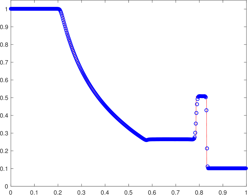
(a) $\rho/10$

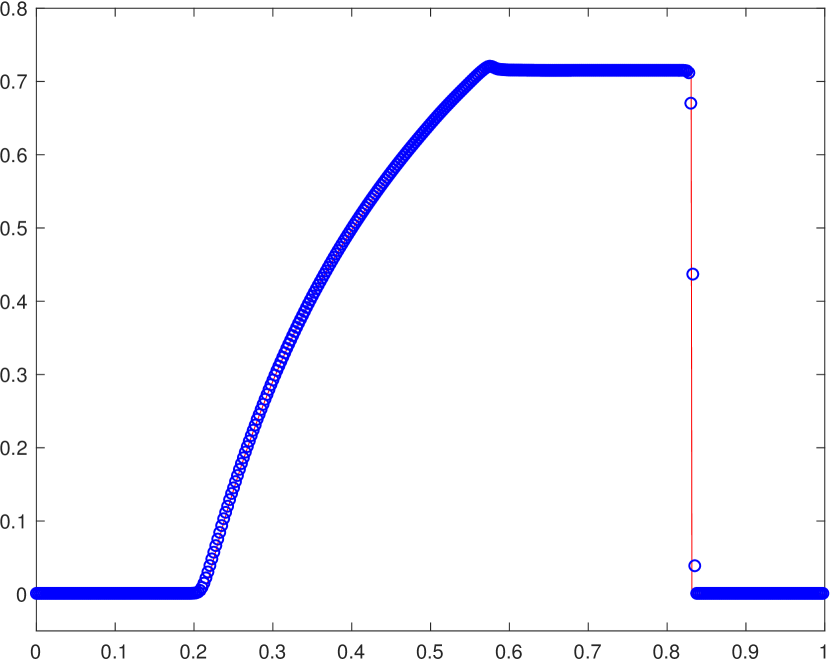
(b) $u$

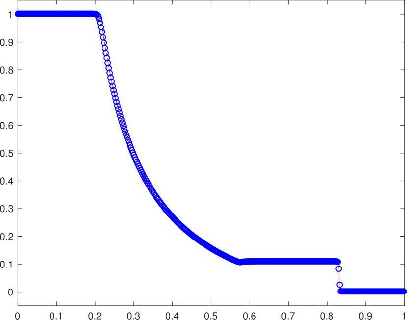
(c) $\frac{3}{40}p$

Figure 5: RP1 in Example 3.2: The solutions at $t=0.4$.

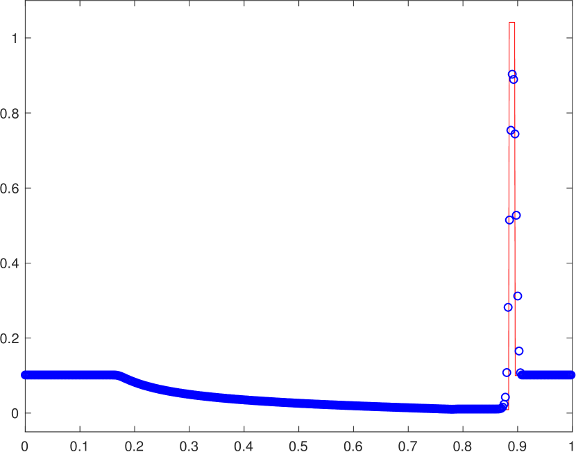
(a) $\rho/7$

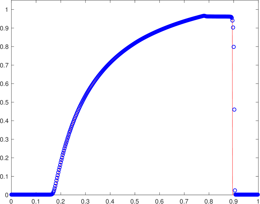
(b) $u$

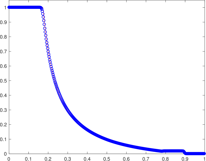
(c) $p/1000$

Figure 6: RP2 in Example 3.2: The solutions at $t=0.4$.

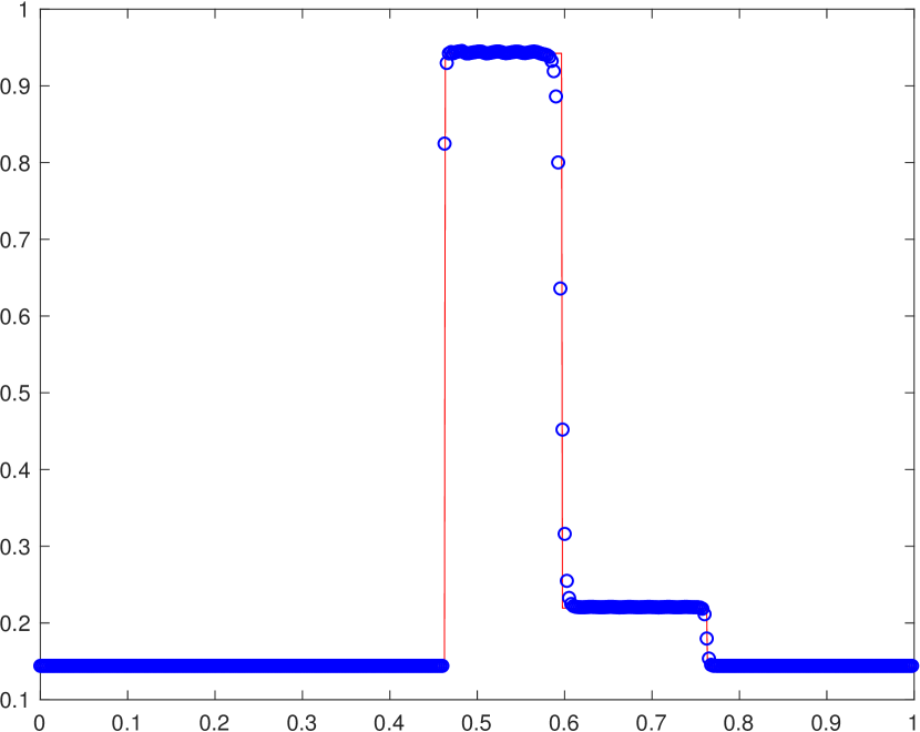
(a) $\rho/7$

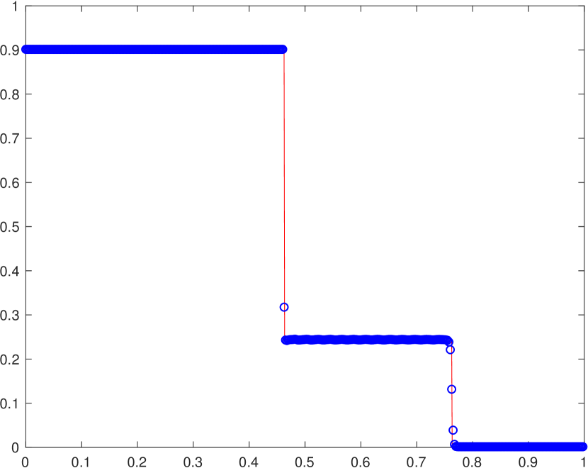
(b) $u$

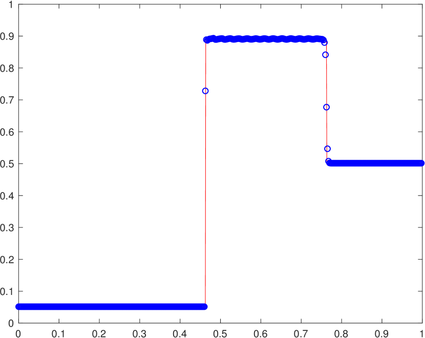
(c) $p/20$

Figure 7: RP3 in Example 3.2: The solutions at $t=0.4$.

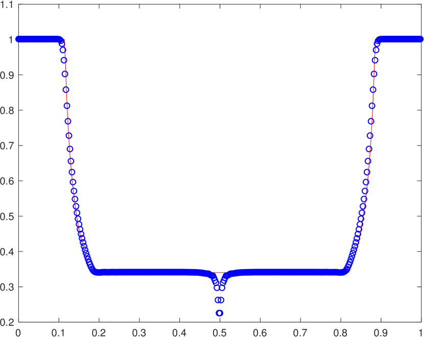
(a) $\rho$

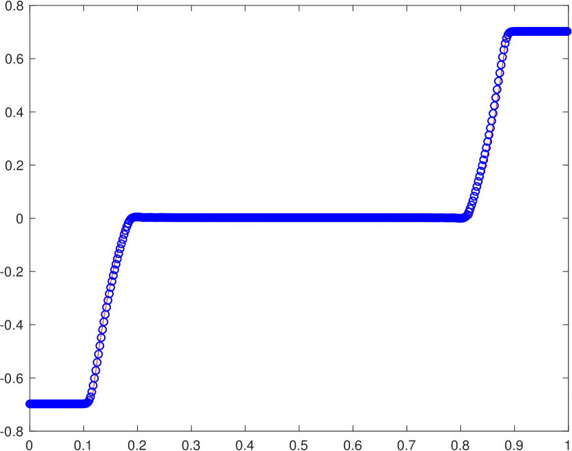
(b) $u$

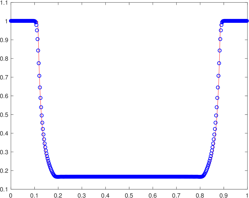
(c) $p/20$

Figure 8: RP4 in Example 3.2: The solutions at $t=0.4$.

Example 3.3 (Density perturbation problem)

This is a more general Cauchy problem obtained by including a density perturbation in the initial data of corresponding Riemann problem in order to test the ability of shock-capturing schemes to resolve small scale flow features, which may give a good indication of the numerical (artificial) viscosity of the scheme. The initial data are given by

$$(\rho,u,p)(x,0)=\begin{cases}(5,\,0,\,50),&x<0.5,\\ (2+0.3\sin(50x),\,0,\,5),&x>0.5.\end{cases}$$

The computational domain is taken as $[0,\,1]$ with the out-flow boundary conditions. Fig. 9 shows the solutions at $t=0.35$ with 400 uniform cells and $\Gamma=5/3$, where the reference solution (“solid line”) are obtained with 2000 uniform cells. It can be seen that our scheme resolves the high frequency waves better than the third order GRP scheme [35].

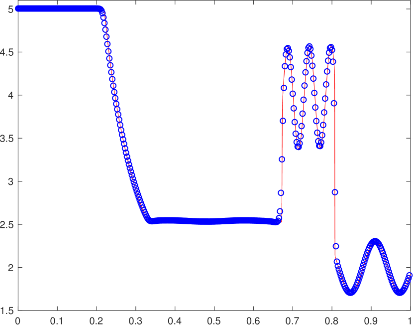
(a) $\rho$

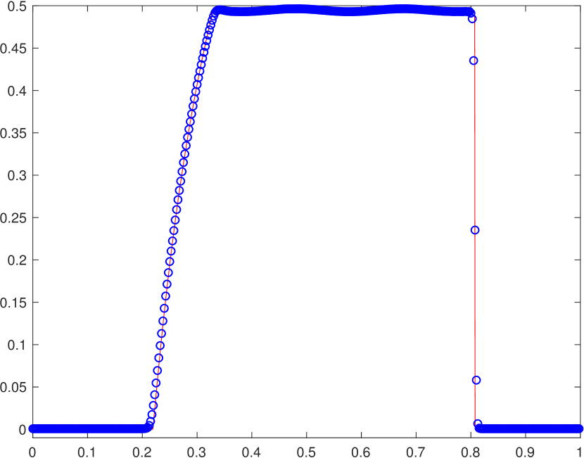
(b) $u$

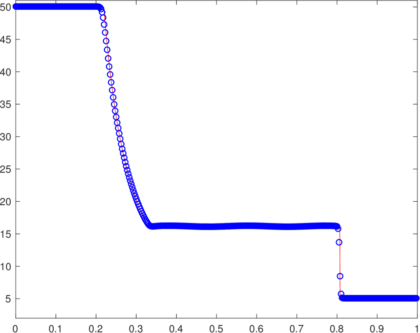
(c) $p$

Figure 9: Example 3.3: The solutions at $t=0.35$.

Example 3.4 (Collision of two blast waves)

The last 1D example simulates the collision of two strong relativistic blast waves. The initial data for this initial-boundary value problems consist of three constant states of an ideal gas with $\Gamma=1.4$, at rest in the domain [0,1] with outflow boundary conditions at $x=0$ and 1. The initial data are given by

$$(\rho,u,p)(x,0)=\begin{cases}(1,\,0,\,10^{3}),&0\leq x<0.1,\\ (1,\,0,\,10^{-2}),&0.1\leq x<0.9,\\ (1,\,0,\,10^{2}),&0.9\leq x<1.0.\end{cases}$$

Two strong blast waves develop and collide, producing a new contact discontinuity. Figs. 10$-$12 show the close-up of solutions at $t=0.43$ with 4000 uniform cells and different $\alpha$, where the exact solution ( “solid line”) are obtained by the exact RP solver with 4000 uniform cells. It is seen that our scheme can well resolve those strong discontinuities, and clearly capture the relativistic wave configurations generated by the collision of the two strong relativistic blast waves.

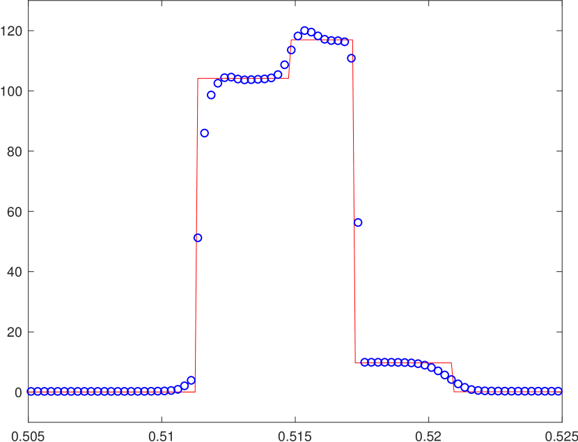
(a) $\rho$

(b) $u$

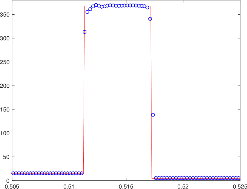
(c) $p$

Figure 10: Example 3.4: Close-up of the solutions at $t=0.43$. $\alpha=\frac{1}{3}$.

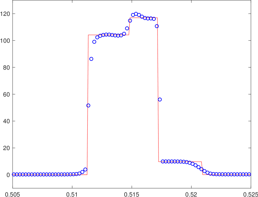
(a) $\rho$

(b) $u$

(c) $p$

Figure 11: Same as Fig. 10 except for $\alpha=\frac{1-6\tau}{3-6\tau}$.

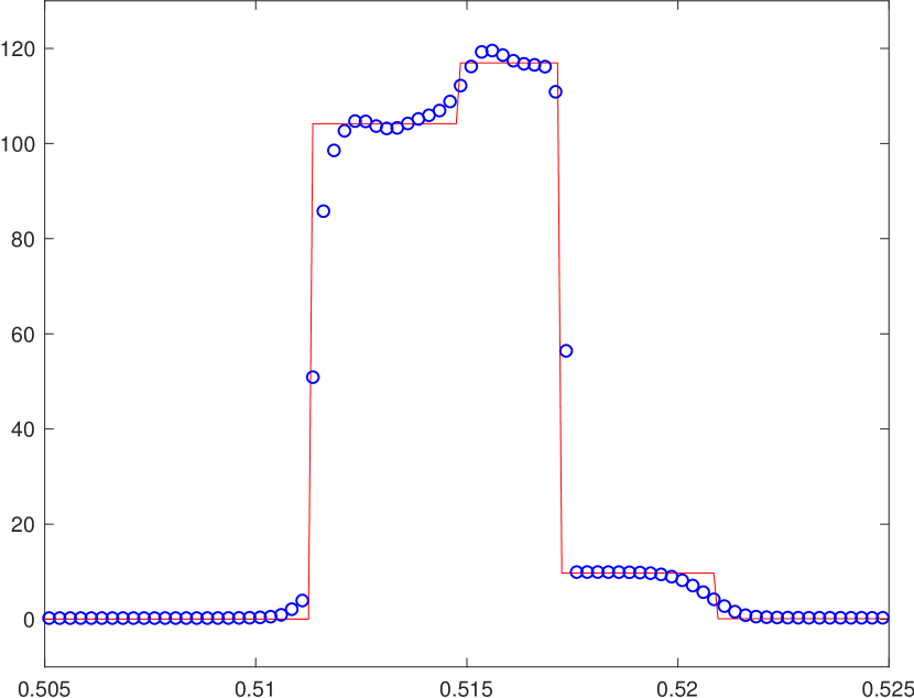
(a) $\rho$

(b) $u$

(c) $p$

Figure 12: Same as Fig. 10 except for $\alpha=\frac{1}{3}+\tau$.

3.2 Two-dimensional case

Unless otherwise stated, the adiabatic index $\Gamma$ is taken as $5/3$ and the parameter $\epsilon$ in the adaptive switch procedure is specified as $0.05$, that is to say, $P_{\mbox{sw}}=1.05$.

Example 3.5 (Smooth problem)

The problem considered here describes a RHD sine wave propagating periodically in the domain $\Omega=[0,2/\sqrt{3}]\times[0,2]$ at an angle of $\alpha=30^{\circ}$ with the $x$-axis. The initial data are taken as

$$\begin{cases}\rho(x,y,0)=1+0.2\sin(2\pi(x\cos\alpha+y\sin\alpha)),\\ u(x,y,0)=0.2,\quad v(x,y,0)=0.2,\quad p(x,y,0)=1.\end{cases}$$

The exact solution can be given by

$$\begin{cases}\rho(x,y,t)=1+0.2\sin(2\pi((x-ut)\cos\alpha+(y-vt)\sin\alpha)),\\ u(x,y,t)=0.2,\quad v(x,y,t)=0.2,\quad p(x,y,t)=1.\end{cases}$$

In our computations, $\tau=\frac{\mu}{\max_{\ell,j,k}\{|\lambda_{\ell}^{1}\left(\overline{\mbox{\boldmath\small$U$}}_{jk}^{n}\right)|\}/{\Delta x^{5/4}}+\max_{\ell,j,k}\{|\lambda_{\ell}^{2}\left(\overline{\mbox{\boldmath\small$U$}}_{jk}^{n}\right)|\}/{\Delta y^{5/4}}}$. Tables 5$-$7 list the errors and convergence rates in $\rho$ at $t=2$ obtained by using our 2D scheme with $N\times N$ uniform cells and different $\alpha$. The results show that our 2D two-stage schemes can have the theoretical orders.

Table 5: The errors and convergence rates for solution at $t=2$. $\alpha=\frac{1}{3}$.

$N$	$l^{1}$ error	order	$l^{2}$ error	order	$l^{\infty}$ error	order
5	8.8639e-02	-	6.4567e-02	-	6.1366e-02	-
10	7.3103e-03	3.6000	5.2506e-03	3.6202	4.8578e-03	3.6591
20	3.4830e-04	4.3915	2.6427e-04	4.3124	2.7917e-04	4.1211
40	1.0722e-05	5.0217	8.2909e-06	4.9943	9.4647e-06	4.8824
80	3.3578e-07	4.9969	2.5428e-07	5.0271	2.9210e-07	5.0180
160	1.0576e-08	4.9887	7.8638e-09	5.0150	9.2428e-09	4.9820

Table 6: Same as Table 5 except for $\alpha=\frac{1-6\tau}{3-6\tau}$.

$N$	$l^{1}$ error	order	$l^{2}$ error	order	$l^{\infty}$ error	order
5	8.8544e-02	-	6.4503e-02	-	6.1296e-02	-
10	7.3094e-03	3.5986	5.2467e-03	3.6199	4.8472e-03	3.6606
20	3.4800e-04	4.3926	2.6414e-04	4.3120	2.7981e-04	4.1146
40	1.0709e-05	5.0222	8.2864e-06	4.9944	9.5006e-06	4.8803
80	3.3590e-07	4.9946	2.5419e-07	5.0268	2.9340e-07	5.0171
160	1.0589e-08	4.9875	7.8733e-09	5.0128	9.3046e-09	4.9788

Table 7: Same as Table 5 except for $\alpha=\frac{1}{3}+\tau$.

$N$	$l^{1}$ error	order	$l^{2}$ error	order	$l^{\infty}$ error	order
5	8.8719e-02	-	6.4621e-02	-	6.1424e-02	-
10	7.3109e-03	3.6011	5.2537e-03	3.6206	4.8660e-03	3.6580
20	3.4852e-04	4.3907	2.6437e-04	4.3127	2.7868e-04	4.1261
40	1.0731e-05	5.0214	8.2950e-06	4.9942	9.4376e-06	4.8840
80	3.3618e-07	4.9964	2.5446e-07	5.0267	2.9111e-07	5.0188
160	1.0593e-08	4.9881	7.8775e-09	5.0136	9.1963e-09	4.9844

Example 3.6 (Riemann problems)

This example solves three 2D Riemann problems to verify the capability of the 2D two-stage scheme in capturing the complex 2D relativistic wave configurations. The computational domain is taken as $[0,1]\times[0,1]$ and divided into $300\times 300$ uniform cells. The output solutions at $t=0.4$ will be plotted with $30$ equally spaced contour lines.

The initial data of RP1 are given by

$$(\rho,u,v,p)(x,0)=\begin{cases}(0.5,\,0.5,\,-0.5,\,0.5),&x>0.5,\,y>0.5,\\ (1,\,0.5,\,0.5,\,5),&x<0.5,\,y>0.5,\\ (3,\,-0.5,\,0.5,\,5),&x<0.5,\,y<0.5,\\ (1.5,\,-0.5,\,-0.5,\,5),&x>0.5,\,y<0.5.\end{cases}$$

It describes the interaction of four contact discontinuities (vortex sheets) with the same sign (the negative sign). Fig. 13 shows the contour of the density and pressure logarithms. The results show that the four initial vortex sheets interact each other to form a spiral with the low density around the center of the domain as time increases, which is the typical cavitation phenomenon in gas dynamics.

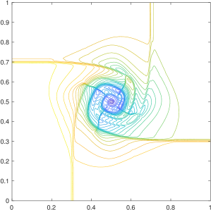
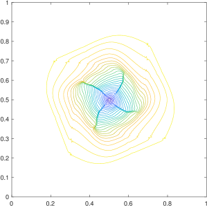
Figure 13: RP1 of Example 3.6: Left: $\log\rho$; right: $\log p$.

The initial data of RP2 are given by

$$(\rho,u,v,p)(x,0)\;=\;\begin{cases}(1,\,0,\,0,\,1),&x>0.5,\,y>0.5,\\ (0.5771,\,-0.3529,\,0,\,0.4),&x<0.5,\,y>0.5,\\ (1,\,-0.3529,\,-0.3529,\,1),&x<0.5,\,y<0.5,\\ (0.5771,\,0,\,-0.3529,\,0.4),&x>0.5,\,y<0.5.\end{cases}$$

Fig. 14 shows the contour of the density and pressure logarithms. The results show that those four initial discontinuities first evolve as four rarefaction waves and then interact each other and form two (almost parallel) curved shock waves perpendicular to the line $x=y$ as time increases.

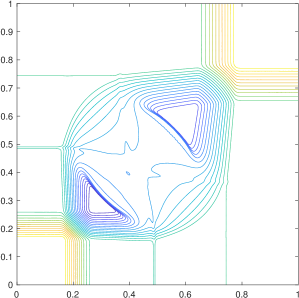
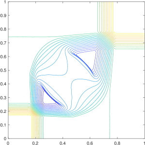
Figure 14: RP2 of Example 3.6: Left: $\log\rho$; right: $\log p$.

The initial data of RP3 are given by

$$(\rho,u,v,p)(x,0)\;=\;\begin{cases}(0.035145216124503,\,0,\,0,\,0.162931056509027),&x>0.5,\,y>0.5,\\ (0.1,\,0.7,\,0.0,\,1.0),&x<0.5,\,y>0.5,\\ (0.5,\,0.0,\,0.0,\,1.0),&x<0.5,\,y<0.5,\\ (0.1,\,0.0,\,0.7,\,1.0),&x>0.5,\,y<0.5,\end{cases}$$

where the left and bottom discontinuities are two contact discontinuities and the top and right are two shock waves with the speed of $0.9345632754$.

Fig. 15 shows the contour of the density and pressure logarithms. We see that four initial discontinuities interact each other and form a “mushroom cloud” around the point $(0.5,0.5)$ as $t$ increases.

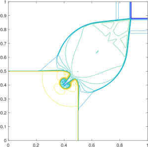
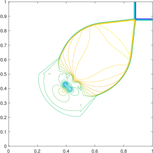
Figure 15: RP3 of Example 3.6: Left: $\log\rho$; right: $\log p$.

Example 3.7 (Double Mach reflection problem)

The double Mach reflection problem for the ideal relativistic fluid with the adiabatic index $\Gamma=1.4$ within the domain $\Omega=[0,4]\times[0,1]$ has been widely used to test the high-resolution shock-capturing scheme, see e.g. [10, 29, 38]. Initially, a right-moving oblique shock with speed $v_{s}=0.4984$ is located at $(x,y)=(1/6,0)$ and makes a $60^{\circ}$ angle with $x$-axis. Thus its position at time $t$ may be given by $h(x,t)=\sqrt{3}(x-1/6)-2v_{s}t$. The left and right states of the shock wave for the primitive variables are given by

$$\mbox{\boldmath\small$V$}(x,y,0)\;=\;\begin{cases}\mbox{\boldmath\small$V$}_{L},&y>h(x,0),\\ \mbox{\boldmath\small$V$}_{R},&y<h(x,0),\end{cases}$$

with $\mbox{\boldmath\small$V$}_{L}=(8.564,0.4247\sin(\pi/3),-0.4247\cos(\pi/3),0.3808)^{T}$ and $\mbox{\boldmath\small$V$}_{R}=(1.4,0.0,0.0,0.0025)^{T}$. The setup of boundary conditions can be found in [10, 29, 38]. Figs. 16$-$18 give the contours of the density and pressure at time $t=5.5$ with $640\times 160$ uniform cells and different $\alpha$. We see that the complicated structure around the double Mach region can be clearly captured.

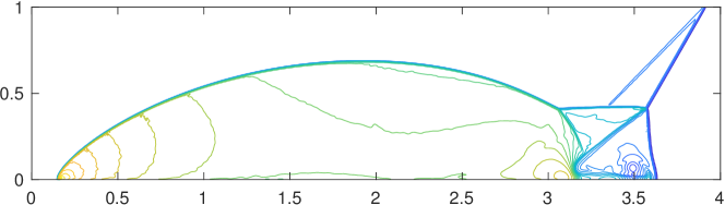
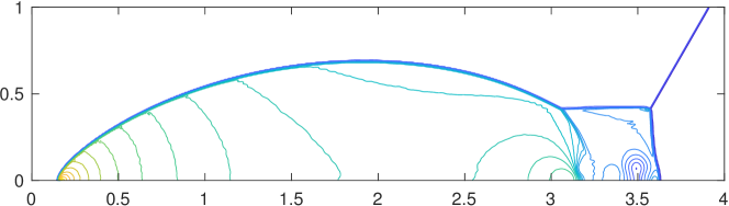
Figure 16: Example 3.7: the contours of $\rho$ (top) and $p$ (bottom) with $30$ equally spaced contour lines. $\alpha=\frac{1}{3}$.

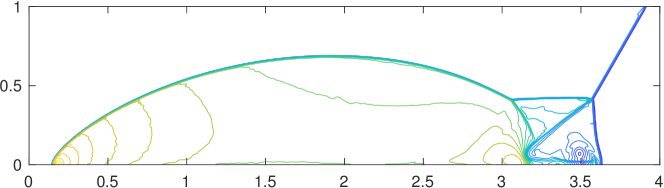
Figure 17: Same as Fig. 16 except for $\alpha=\frac{1-6\tau}{3-6\tau}$.

Figure 18: Same as Fig. 16 except for $\alpha=\frac{1}{3}+\tau$.

Example 3.8 (Shock-bubble interaction problems)

The final example considers two shock-bubble interaction problems within the computational domain $[0,325]\times[0,90]$. Their detailed setup can be found in [29].

For the first shock-bubble interaction problem, the left and right states of planar shock wave moving left are given by

$$\mbox{\boldmath\small$V$}(x,y,0)=\begin{cases}(1,0,0,0.05)^{T},&x<265,\\ (1.865225080631180,-0.196781107378299,0,0.15)^{T},&x>265,\end{cases}$$

and the bubble is described as $\mbox{\boldmath\small$V$}(x,y,0)=(0.1358,0,0,0.05)^{T}$ if $\sqrt{(x-215)^{2}+(y-45)^{2}}\leq 25$. The setup of the second shock-bubble problem is the same as the first, except for that the initial state of the fluid in the bubble is replaced with $\mbox{\boldmath\small$V$}(x,y,0)=(3.1538,0,0,0.05)^{T}$ if $\sqrt{(x-215)^{2}+(y-45)^{2}}\leq 25$.

Fig. 19 gives the contour plots of the density at $t=90,180,270,360,450$ (from top to bottom) of the first shock-bubble interaction problem, obtained by using our scheme with $325\times 90$ uniform cells. Fig. 20 presents the contour plots of the density at several moments $t=100,200,300,400,500$ (from top to bottom) of the second shock-bubble interaction problem, obtained by using our 2D two-stage scheme with $325\times 90$ uniform cells. Those results show that the discontinuities and some small wave structures including the curling of the bubble interface are captured well and accurately, and at the same time, the multi-dimensional wave structures are also resolved clearly. Those plots are also clearly displaying the dynamics of the interaction between the shock wave and the bubble and obviously different wave patterns of the interactions between those shock waves and the bubbles.

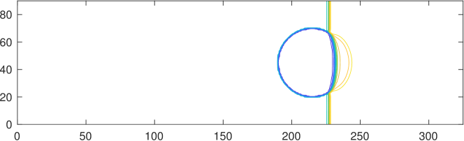
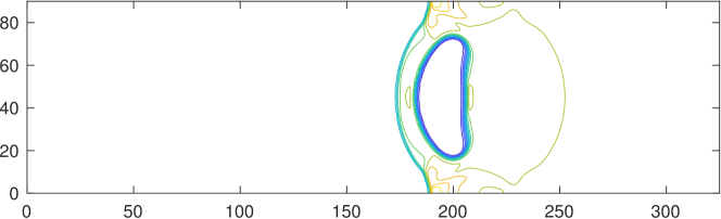
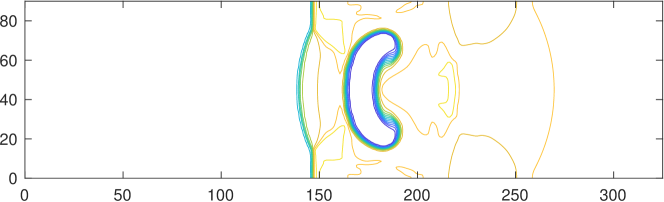
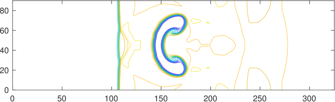
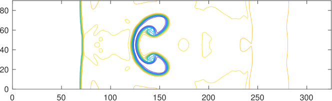
Figure 19: The first problem of Example 3.8: the contours of $\rho$ at $t=90,180,270,360,450$ with $15$ equally spaced contour lines.

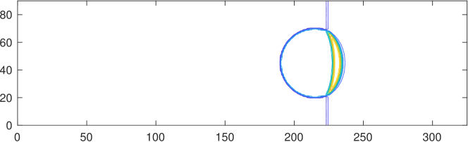
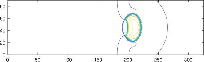
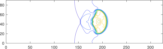
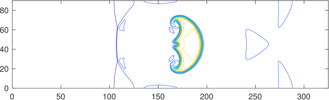
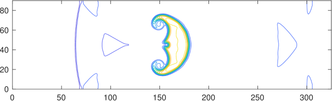
Figure 20: The second problem of Example 3.8: the contours of $\rho$ at $t=100,200,300,400,500$ with $15$ equally spaced contour lines.

4 Conclusions

The paper studied the two-stage fourth-order accurate time discretization [18] and its application to the special relativistic hydrodynamical (RHD) equations. It was shown that new two-stage fourth-order accurate time discretizations could be proposed. The local “quasi 1D” GRP (generalized Riemann problem) of the special RHD equations was also analytically resolved. With the aid of the direct Eulerian GRP methods [37, 38] and the analytical resolution of local “quasi 1D” GRP as well as the adaptive primitive-conservative scheme [17], the two-stage fourth-order accurate time discretizations were successfully implemented for the 1D and 2D special RHD equations. The adaptive primitive-conservative scheme was used to reduce the spurious solution generated by the conservative scheme across the contact discontinuity. Several numerical experiments were conducted to demonstrate the performance and accuracy as well as robustness of our schemes.

Appendix A The resolution of quasi 1D GRP of special RHD equations

The equation (26) can be equivalently written into the primitive variable form

$$\partial_{t}\mbox{\boldmath\small$V$}+\widetilde{\mbox{\boldmath\small$A$}}(\mbox{\boldmath\small$V$})\partial_{x}\mbox{\boldmath\small$V$}=\mbox{\boldmath\small$C$}=[C_{1},C_{2},C_{3},C_{4}]^{T},$$ (30)

where

$$C_{4}= \frac{1}{1-(u^{2}+v^{2})c_{s}^{2}}[h_{4}(\Gamma-1+(u^{2}+v^{2})c_{s}^{2})-\frac{\Gamma-1}{W}h_{1}-(c_{s}^{2}+\Gamma-1)(uh_{2}+vh_{3})],$$

$$C_{2}= \frac{1}{\rho hW^{2}}[h_{2}-uh_{4}-uC_{4}],\ C_{3}=\frac{1}{\rho hW^{2}}[h_{3}-vh_{4}-vC_{4}],C_{1}=\frac{h_{1}}{W}-W^{2}\rho(uC_{2}+vC_{3}),$$

and $\mbox{\boldmath\small$h$}:=(h_{1},\,h_{2},\,h_{3},\,h_{4})^{T}$ denotes the right hand of (26).

For the matrix $\widetilde{\mbox{\boldmath\small$A$}}(\mbox{\boldmath\small$V$})$ given in (24), its eigenvalues and (right and left) eigenvector matrices can be easily given as follows

$$\lambda_{1}=\dfrac{u(1-c_{s}^{2})-c_{s}W^{-1}H^{1/2}}{1-(u^{2}+v^{2})c_{s}^{2}},\ \lambda_{2}=\lambda_{3}=u,\ \lambda_{4}=\dfrac{u(1-c_{s}^{2})+c_{s}W^{-1}H^{1/2}}{1-(u^{2}+v^{2})c_{s}^{2}},$$ (31)

$$\widetilde{\mbox{\boldmath\small$R$}}(\mbox{\boldmath\small$V$})=\begin{pmatrix}\dfrac{\rho W^{2}}{c_{s}}&1&0&\dfrac{\rho W^{2}}{c_{s}}\\ -WH^{1/2}&0&0&WH^{1/2}\\ \dfrac{v(uWH^{1/2}-c_{s})}{1-u^{2}}&0&1&-\dfrac{v(uWH^{1/2}+c_{s})}{1-u^{2}}\\ \rho hc_{s}W^{2}&0&0&\rho hc_{s}W^{2}\end{pmatrix},$$ (32)

and

$$\widetilde{\mbox{\boldmath\small$R$}}^{-}(\mbox{\boldmath\small$V$})=\frac{1}{|\widetilde{\mbox{\boldmath\small$R$}}(\mbox{\boldmath\small$V$})|}\begin{pmatrix}0&-\rho hc_{s}W^{2}&0&WH^{1/2}\\ |\widetilde{\mbox{\boldmath\small$R$}}(\mbox{\boldmath\small$V$})|&0&0&\dfrac{-2\rho W^{3}H^{1/2}}{c_{s}}\\ 0&\dfrac{2uv\rho hc_{s}W^{3}H^{1/2}}{1-u^{2}}&|\widetilde{\mbox{\boldmath\small$R$}}(\mbox{\boldmath\small$V$})|&\dfrac{2vc_{s}WH^{1/2}}{1-u^{2}}\\ 0&\rho hc_{s}W^{2}&0&WH^{1/2}\end{pmatrix},$$ (33)

where $|\widetilde{\mbox{\boldmath\small$R$}}(\mbox{\boldmath\small$V$})|=2\rho hc_{s}W^{3}H^{1/2}$.

For the sake of brevity, we will omit the notation $(\cdot)_{*}$ widely used in the direct Eulerian GRP methods [8, 9, 30, 35, 36, 37, 38].

A.1 Resolution of shock wave

It is very similar to that given in [38] except for $(3.43)$, because the source terms affect $\frac{D}{Ds}:=\partial_{t}+s\cdot\partial_{x}$ as follows

$$\begin{cases}\frac{Du}{Ds}=\frac{1-us}{1-u^{2}}\cdot\frac{Du}{Dt}+\frac{u-s}{1-u^{2}}\cdot\frac{H}{\rho hc_{s}^{2}}\cdot\frac{Dp}{Dt}+\frac{s-u}{(1-u^{2})}\cdot\left[u\,C_{2}+\frac{H}{\rho hc_{s}^{2}}C_{4}\right],\\ \frac{Dp}{Ds}=\frac{1-us}{1-u^{2}}\cdot\frac{Dp}{Dt}+\frac{u-s}{1-u^{2}}\cdot\rho hW^{2}\cdot\frac{Du}{Dt}+\frac{s-u}{(1-u^{2})}\cdot\left[u\,C_{4}+\rho hW^{2}C_{2}\right],\end{cases}$$

where $s$ is the shock speed. The present result is given in the following lemma.

Lemma A.1

The limiting values of $(Du/Dt)_{*}$ and $(Dp/Dt)_{*}$ satisfy

$$a_{R}\,\left(\frac{Du}{Dt}\right)_{*}\;+\;b_{R}\,\left(\frac{Dp}{Dt}\right)_{*}\;=\;d_{R},$$ (34)

where

$$A_{us}=uC_{2}+\frac{H}{\rho hc_{s}^{2}}C_{4},\ A_{ps}=\rho hW^{2}C_{2}+uC_{4},$$

and

$$\begin{cases}a_{R}=A_{u}+\frac{u-s}{1-us}\rho hW^{2}A_{p},\\ b_{R}=A_{p}+\frac{u-s}{1-us}\frac{H}{\rho hc_{s}^{2}}A_{u},\\ d_{R}=\frac{1-u^{2}}{1-us}A_{rhs}+\frac{u-s}{1-us}\cdot\left(A_{us}A_{u}+A_{ps}A_{p}\right),\end{cases}$$

with $A_{u}$ and $A_{p}$ defined in [38].

A.2 Resolution of centered rarefaction wave

With the help of $\widetilde{\mbox{\boldmath\small$R$}}(\mbox{\boldmath\small$V$})$, we can easily derive the Riemann invariants

$$\begin{cases}\mbox{for}\;\lambda_{1}:&\psi_{+},\,S,\,V,\\ \mbox{for}\;\lambda_{2}(\lambda_{3}):&u,\,p,\\ \mbox{for}\;\lambda_{4}:&\psi_{-},\,S,\,V,\end{cases}$$ (35)

where $V=hvW$, $\psi_{\pm}=\dfrac{1}{2}\ln\left(\dfrac{1+u}{1-u}\right)\pm\int^{p}\varphi dp=\dfrac{1}{2}\ln\left(\dfrac{1+u}{1-u}\right)\pm\int^{\rho}\tilde{\varphi}d\rho$, and

$$\varphi=\dfrac{H^{1/2}}{\rho hc_{s}W(1-u^{2})}=\dfrac{\sqrt{h^{2}+V^{2}(1-c_{s}^{2})}}{\rho c_{s}(h^{2}+V^{2})},\quad\tilde{\varphi}=hc_{s}^{2}\varphi.$$ (36)

The Riemann invariants $\psi_{\pm}$ satisfy

$$d\psi_{\pm}=\dfrac{1}{1-u^{2}}du\pm\left[\varphi dp+K_{S}dS+K_{V}dV\right],$$ (37)

where

$$\begin{cases}K_{S}=\tilde{K}_{S}-\varphi\frac{\partial p}{\partial S},\\ K_{V}=\frac{\partial}{\partial V}\int^{p}\varphi dp,\\ \tilde{K}_{S}=\frac{\partial}{\partial S}\int^{\rho}\tilde{\varphi}d\rho,\\ \frac{\partial\varphi}{\partial V}=\varphi V\left(\frac{1-c_{s}^{2}}{h^{2}+V^{2}(1-c_{s}^{2})}-\frac{2}{h^{2}+V^{2}}\right).\end{cases}$$ (38)

Note that the lower limits of two integrals in (38) may be $\rho_{0}>0$ and $p_{0}>0$, respectively.

Thanks to the thermodynamic relation $TdS=de-\frac{p}{\rho^{2}}d\rho$ and the $\Gamma$-law $p=(\Gamma-1)\rho e$, one has

$$TdS=\frac{1}{(\Gamma-1)\rho}\left(dp-hc_{s}^{2}d\rho\right).$$

Together with $V=hWv$, (37) and (30), we obtain

$$\begin{cases}\partial_{t}\psi_{-}+\lambda_{1}\partial_{x}\psi_{-}=B_{1}-(\lambda_{1}-u)\cdot(K_{S}\partial_{x}S+K_{V}\partial_{x}V),\\ \partial_{t}\psi_{+}+\lambda_{4}\partial_{x}\psi_{+}=B_{2}+(\lambda_{4}-u)\cdot(K_{S}\partial_{x}S+K_{V}\partial_{x}V),\\ T(\partial_{t}S+u\partial_{x}S)=B_{3},\\ \partial_{t}V+u\partial_{x}V=B_{4},\\ \end{cases}$$ (39)

where

$$\begin{cases}B_{1}=\frac{1}{1-u^{2}}C_{2}-\varphi C_{4}-\frac{K_{S}}{T}B_{3}-K_{V}B_{4},\\ B_{2}=\frac{1}{1-u^{2}}C_{2}+\varphi C_{4}+\frac{K_{S}}{T}B_{3}+K_{V}B_{4},\\ B_{3}=\frac{1}{(\Gamma-1)\rho}\cdot\left(C_{4}-hc_{s}^{2}C_{1}\right)=\frac{1}{\rho}\cdot\left(h_{4}-uh_{2}-vh_{3}-\frac{h}{W}h_{1}\right),\\ B_{4}=-\frac{hv}{\rho}h_{1}+\frac{1}{\rho W}h_{3}.\end{cases}$$

Based on the above preparation, following the procedure in [38], one can get the main result of resolving the left rarefaction waves.

Lemma A.2

The limiting values of $(Du/Dt)_{*}$ and $(Dp/Dt)_{*}$ satisfy

$$a_{L}\,\left(\frac{Du}{Dt}\right)_{*}\;+\;b_{L}\,\left(\frac{Dp}{Dt}\right)_{*}\;=\;d_{L},$$ (40)

with

$$\begin{cases}a_{L}=\frac{1}{1-u^{2}},\ \ b_{L}=\varphi,\\ d_{L}=\dfrac{\lambda_{4}-u}{\lambda_{4}-\lambda_{1}}\left(\frac{\partial t}{\partial\alpha}\right)^{-1}\frac{\partial\psi_{+}}{\partial\alpha}+\dfrac{u-\lambda_{1}}{\lambda_{4}-\lambda_{1}}\left[B_{2}+(\lambda_{4}-u)(K_{S}\partial_{x}S+K_{V}\partial_{x}V)\right]-\frac{K_{S}}{T}B3-K_{V}B_{4},\end{cases}$$

where $\partial_{x}S$, $\partial_{x}V$ and $\frac{\partial\psi_{+}}{\partial\alpha}$ are calculated by (42), (43) and (A.2), respectively.

• Since

  $$T\frac{\partial S}{\partial\alpha}= \frac{\partial t}{\partial\alpha}\cdot\left[B_{3}+(\lambda_{1}-u)T\frac{\partial S}{\partial x}\right],\ T\frac{\partial S}{\partial\beta}=\frac{\partial t}{\partial\beta}\cdot\left[B_{3}+(\lambda_{4}-u)T\frac{\partial S}{\partial x}\right],$$ (41)

  taking $\alpha$-derivative to (41) gives

  $$\frac{\partial}{\partial\alpha}\left(T\frac{\partial S}{\partial\beta}\right)=\frac{\partial^{2}t}{\partial\beta\partial\alpha}\cdot\left[B_{3}+(\lambda_{4}-u)T\frac{\partial S}{\partial x}\right]+\frac{\partial t}{\partial\beta}\cdot\frac{\partial}{\partial\alpha}\left[B_{3}+(\lambda_{4}-u)T\frac{\partial S}{\partial x}\right].$$

  Together with

  $$\frac{\partial}{\partial\beta}\left(T\frac{\partial S}{\partial\alpha}\right)=\frac{\partial T}{\partial\beta}\frac{\partial S}{\partial\alpha}+\frac{\partial^{2}S}{\partial\beta\partial\alpha},\ \frac{\partial}{\partial\alpha}\left(T\frac{\partial S}{\partial\beta}\right)=\frac{\partial T}{\partial\alpha}\frac{\partial S}{\partial\beta}+\frac{\partial^{2}S}{\partial\beta\partial\alpha},$$

  setting $\alpha=0$ gives

  $$\frac{\partial}{\partial\beta}\left(T\frac{\partial S}{\partial\alpha}(0,\beta)\right)=\left[\frac{\partial\ln T}{\partial\beta}+\frac{(\lambda_{4}-u)}{(\lambda_{4}-\lambda_{1})(\lambda_{1}-u)}\right]\bigg{|}_{\alpha=0}\left(T\frac{\partial S}{\partial\alpha}(0,\beta)\right)+\frac{B_{3}}{u-\lambda_{1}}\bigg{|}_{\alpha=0}\frac{\partial t}{\partial\alpha}(0,\beta).$$

  Hence it holds

  $$\left(\frac{\partial t}{\partial\alpha}\bigg{|}_{L}\right)^{-1}\left(T\frac{\partial S}{\partial\alpha}\right)\bigg{|}_{\alpha=0}= \dfrac{T}{T_{L}}\bigg{|}_{\alpha=0}\mbox{exp}\left(\int^{\beta}_{\beta_{L}}\frac{(\lambda_{4}-u)}{(\lambda_{4}-\omega)(\omega-u)}d\omega\right)\Bigg{[}B_{3}^{L}+(\lambda_{1}-u)|_{L}T_{L}S^{\prime}_{L}$$

  $$+\int^{\beta}_{\beta_{L}}\frac{B_{3}}{u-\beta}\dfrac{\partial_{\alpha}t(0,\beta)}{\partial_{\alpha}t(0,\beta_{L})}\dfrac{T_{L}}{T}\mbox{exp}\left(\int^{\beta}_{\beta_{L}}\frac{(\lambda_{4}-u)}{(\lambda_{4}-\omega)(u-\omega)}d\omega\right)d\beta\Bigg{]},$$

  where

  $$\dfrac{\partial_{\alpha}t(0,\beta)}{\partial_{\alpha}t(0,\beta_{L})}=\exp\left(\int^{\beta}_{\beta_{L}}\frac{1}{(\lambda_{4}-\omega)}d\omega\right),\quad\dfrac{T}{T_{L}}\bigg{|}_{\alpha=0}=\dfrac{(hc_{s}^{2})|_{\alpha=0}}{(hc_{s}^{2})|_{L}},$$

  and the subscript $L$ represents $(0,\beta_{L})$. Therefore, one gets

  $$\left(T\frac{\partial S}{\partial x}\right)\bigg{|}_{\alpha=0}\;=\;\frac{1}{u-\lambda_{1}}\bigg{|}_{\alpha=0}\cdot\left[B_{3}-\left(\frac{\partial t}{\partial\alpha}\right)^{-1}T\frac{\partial S}{\partial\alpha}\right]\bigg{|}_{\alpha=0}.$$ (42)

  Similarly, one can calculate $\frac{\partial V}{\partial x}(0,\beta)$ as

  $$\frac{\partial V}{\partial x}(0,\beta)\;=\;\frac{1}{u-\lambda_{1}}\bigg{|}_{\alpha=0}\cdot\left[B_{4}-\left(\frac{\partial t}{\partial\alpha}\right)^{-1}\frac{\partial V}{\partial\alpha}\right]\bigg{|}_{\alpha=0},$$ (43)

  where

  $$\left(\frac{\partial t}{\partial\alpha}\bigg{|}_{L}\right)^{-1}\frac{\partial V}{\partial\alpha}(0,\beta)= \mbox{exp}\left(\int^{\beta}_{\beta_{L}}\frac{(\lambda_{4}-u)}{(\lambda_{4}-\omega)(\omega-u)}d\omega\right)\Bigg{[}B_{4}^{L}+(\lambda_{1}-u)|_{L}V^{\prime}_{L},$$

  $$+\int^{\beta}_{\beta_{L}}\frac{B_{4}}{u-\beta}\dfrac{\partial_{\alpha}t(0,\beta)}{\partial_{\alpha}t(0,\beta_{L})}\mbox{exp}\left(\int^{\beta}_{\beta_{L}}\frac{(\lambda_{4}-u)}{(\lambda_{4}-\omega)(u-\omega)}d\omega\right)d\beta\Bigg{]}.$$

Finally, let us calculate $\frac{\partial\psi_{+}}{\partial\alpha}(0,\beta)$. Since

$$\frac{\partial\psi_{+}}{\partial\alpha}= \frac{\partial t}{\partial\alpha}\cdot\left[\frac{D_{+}}{Dt}\psi_{+}+(\lambda_{1}-\lambda_{4})\frac{\partial\psi_{+}}{\partial x}\right],\ \frac{\partial\psi_{+}}{\partial\beta}=\frac{\partial t}{\partial\beta}\cdot\frac{D_{+}}{Dt}\psi_{+},$$

where $\frac{D_{+}}{Dt}=\frac{\partial}{\partial t}+\lambda_{4}\frac{\partial}{\partial x}$, setting $\alpha=0$ gives

$$\frac{\partial}{\partial\beta}\left(\frac{\partial\psi_{+}}{\partial\alpha}(0,\beta)\right)=\bigg{(}\dfrac{1}{\lambda_{4}-\lambda_{1}}\frac{\partial t}{\partial\alpha}\cdot\left[B_{2}+(\lambda_{4}-u)\cdot(K_{S}\partial_{x}S+K_{V}\partial_{x}V)\right]\bigg{)}\bigg{|}_{\alpha=0}.$$

Some tedious manipulations yield

$$\left(\frac{\partial t}{\partial\alpha}\bigg{|}_{L}\right)^{-1} \frac{\partial\psi_{+}}{\partial\alpha}(0,\beta)=B_{2}^{L}+(\lambda_{1}-u)|_{L}\cdot\left[\dfrac{K_{S}^{L}}{T_{L}}T_{L}S^{\prime}_{L}+K_{V}^{L}V^{\prime}_{L}\right]$$

$$+(\lambda_{1}-\lambda_{4})|_{L}\cdot\left[\dfrac{1}{1-u_{L}^{2}}u^{\prime}_{L}+\varphi_{L}p^{\prime}_{L}\right]$$

$$+\int^{\beta}_{\beta_{L}}\frac{1}{\lambda_{4}-\omega}\dfrac{\partial_{\alpha}t(0,\omega)}{\partial_{\alpha}t(0,\beta_{L})}\left[B_{2}+(\lambda_{4}-u)\cdot(K_{S}\partial_{x}S+K_{V}\partial_{x}V)\right]\;d\omega.$$ (44)

Together with (37) and (39), the proof of Lemma A.2 is completed.       

A.3 Time derivatives of solutions at singularity point

Solving the $2\times 2$ linear system formed by (34) in Lemma A.1 and (40) in Lemma A.2 may give the values of the total derivatives of the normal velocity and the pressure and the the limiting values of time derivatives $\,(\partial u/\partial t)_{*}\,$ and $\,(\partial p/\partial t)_{*}$.

A.3.1 General case

Theorem A.3

The limiting value $\,(\partial u/\partial t)_{*}\,$ and $\,(\partial p/\partial t)_{*}\,$ are calculated as follows.

• (Nonsonic case) The limiting values of time derivatives $\,(\partial u/\partial t)_{*}\,$ and $\,(\partial p/\partial t)_{*}\,$ can be calculated as

  $$\left\{\begin{array}[]{l}\partial_{t}u=\frac{1}{1-u^{2}}\left[\frac{Du}{Dt}+\frac{uH}{\rho hc_{s}^{2}}\frac{Dp}{Dt}-u\cdot\left(uC_{2}+\frac{H}{\rho hc_{s}^{2}}C_{4}\right)\right],\\ \partial_{t}p=\frac{1}{1-u^{2}}\left[\frac{Dp}{Dt}+u\rho hW^{2}\frac{Du}{Dt}-u\cdot\left(\rho hW^{2}C_{2}+uC_{4}\right)\right].\end{array}\right.$$

• (Sonic case) If assuming that the $t$-axis is located inside the rarefaction wave associated with the $\,\lambda_{1}\,$ characteristic family, then

  $$\begin{cases}\partial_{t}u=\frac{1-u^{2}}{2}\left[\frac{\lambda_{4}}{\lambda_{4}-u}\cdot\Big{(}d_{L}(0)-\varphi C_{4}\Big{)}+\frac{\lambda_{4}-2u}{\lambda_{4}-u}\cdot\frac{1}{1-u^{2}}C_{2}\right],\\ \partial_{t}p=\frac{1}{2\varphi}\left[\frac{\lambda_{4}}{\lambda_{4}-u}\cdot\Big{(}d_{L}(0)-\dfrac{1}{1-u^{2}}C_{2}\Big{)}+\frac{\lambda_{4}-2u}{\lambda_{4}-u}\cdot\varphi C_{4}\right].\end{cases}$$

• Here consider the sonic case. As the $t$-axis is located inside the rarefaction wave associated with the $\,\lambda_{1}\,$ characteristic family, then we have $\,\lambda_{1}=0$.

  Thanks to

  $$\frac{D_{-}u}{Dt}-C_{2}=\Phi\cdot\left(\frac{D_{-}p}{Dt}-C_{4}\right),$$

  with $\Phi=\frac{H^{1/2}}{\rho hc_{s}W}=(1-u^{2})\varphi$ and $\frac{D_{-}}{Dt}:=\frac{\partial}{\partial t}+\lambda_{1}\frac{\partial}{\partial x}$, one has

  $$\dfrac{1}{1-u^{2}}\partial_{t}u-\varphi\partial_{t}p=\dfrac{1}{1-u^{2}}C_{2}-\varphi C_{4}.$$ (45)

  On the other hand, together with (40), $\frac{D}{Dt}=\frac{u-\lambda_{1}}{\lambda_{4}-\lambda_{1}}\frac{D_{-}}{Dt}+\frac{\lambda_{4}-u}{\lambda_{4}-\lambda_{1}}\frac{D_{+}}{Dt}$ and

  $$\frac{D_{+}u}{Dt}-C_{2}=-\Phi\cdot\left(\frac{D_{+}p}{Dt}-C_{4}\right),$$

  with $\frac{D_{+}}{Dt}:=\frac{\partial}{\partial t}+\lambda_{4}\frac{\partial}{\partial x}$, one gets

  $$\dfrac{1}{1-u^{2}}\partial_{t}u+\varphi\partial_{t}p=\dfrac{\lambda_{4}}{\lambda_{4}-u}d_{L}(0)-\dfrac{u}{\lambda_{4}-u}\cdot[\dfrac{1}{1-u^{2}}C_{2}+\varphi C_{4}].$$ (46)

  With the help of (45) and (46), the proof can be completed.       

Theorem A.4

The limiting value $\,(\partial\rho/\partial t)_{*}\,$ and $\,(\partial v/\partial t)_{*}\,$ are calculated as follows.

• If $\,u_{*}>0\,$, they are obtained by

  $$\left(\frac{\partial\rho}{\partial t}\right)_{*}= \frac{1}{hc^{2}_{1*}}\cdot\left[\left(\frac{\partial p}{\partial t}\right)_{*}-\frac{1}{T}\left(\frac{\partial p}{\partial S}\right)_{\rho}\left(B_{3}-u_{*}\left(T\frac{\partial S}{\partial x}\right)_{*}\right)\right],$$

  $$\left(\frac{\partial v}{\partial t}\right)_{*}= \frac{-1}{hW(1+W^{2}v^{2})}\Big{[}\,Wv\partial_{t}h+VW^{2}u\partial_{t}u+u\partial_{x}V-B_{4}\,\Big{]},$$

  where $\partial_{x}V$ is given in (43) and $dh=\frac{\Gamma}{\Gamma-1}\left(\frac{1}{\rho}dp-\frac{p}{\rho^{2}}d\rho\right)$.

• If $\,u_{*}<0\,$, they are given by

  $$\left(\frac{\partial\rho}{\partial t}\right)_{*}=\dfrac{1}{s-u}\left[s\left(\frac{D\rho}{Dt}\right)_{*}-u\left(\frac{D\rho}{Ds}\right)_{*}\right],$$

  $$\left(\frac{\partial v}{\partial t}\right)_{*}=\frac{-1}{hW(1+W^{2}v^{2})}\Big{[}\,Wv\partial_{t}h+VW^{2}u\partial_{t}u+u\partial_{x}V-B_{4}\,\Big{]},$$

  where $\left(\frac{D\rho}{Ds}\right)_{*}$ is given in [38, (3.39)], and

  $$\begin{cases}\left(\frac{D\rho}{Dt}\right)_{*}=\dfrac{1}{hc^{2}}\cdot\left(\left(\frac{Dp}{Dt}\right)_{*}-C_{4}\right)+C_{1},\\ \partial_{x}V=\frac{1}{s-u_{*}}\cdot\Big{[}B_{4}^{R}+(s-u_{R})\partial_{x}V_{R}-B_{4}\Big{]},\\ \partial_{x}V_{R}=\Big{[}Wv\partial_{x}h+VW^{2}u\partial_{x}u+hW(1+W^{2}v^{2})\partial_{x}v\Big{]}\Big{|}_{R}.\end{cases}$$

A.3.2 Acoustic case

When $\mbox{\boldmath\small$U$}_{L}=\mbox{\boldmath\small$U$}_{R}=\mbox{\boldmath\small$U$}_{*}$ and $\mbox{\boldmath\small$U$}^{\prime}_{L}\neq\mbox{\boldmath\small$U$}^{\prime}_{R}$, we meet the acoustic case.

Theorem A.5

If assuming $(\lambda_{1})_{*}<0$ and $(\lambda_{4})_{*}>0$, then $(\partial u/\partial t)_{*}$ and $(\partial p/\partial t)_{*}$ can be calculated by

$$\begin{cases}\left(\frac{\partial u}{\partial t}\right)_{*}=\frac{1}{\lambda_{4}-\lambda_{1}}\Big{(}\lambda_{4}\cdot[C_{2}^{L}+(M+\lambda_{1}-u)|_{L}u^{\prime}_{L}-N_{u}^{L}p^{\prime}_{L}]-\lambda_{1}\cdot[C_{2}^{R}+(M+\lambda_{4}-u)|_{R}u^{\prime}_{R}-N_{u}^{L}p^{\prime}_{R}]\Big{)},\\ \left(\frac{\partial p}{\partial t}\right)_{*}=\frac{1}{\lambda_{4}-\lambda_{1}}\Big{(}\lambda_{4}\cdot[C_{4}^{L}+(M+\lambda_{1}-u)|_{L}p^{\prime}_{L}-N_{p}^{L}u^{\prime}_{L}]-\lambda_{1}\cdot[C_{4}^{R}+(M+\lambda_{4}-u)|_{R}p^{\prime}_{R}-N_{p}^{L}u^{\prime}_{R}]\Big{)},\end{cases}$$

where

$$M=u-\dfrac{\lambda_{4}+\lambda_{1}}{2},\quad N_{u}=\dfrac{\lambda_{4}-\lambda_{1}}{2}\Phi,\quad N_{p}=\dfrac{\lambda_{4}-\lambda_{1}}{2}\Phi^{-1}.$$

With the aid of the EOS $p=p(\rho,S)$, $(\partial\rho/\partial t)_{*}$ is calculated by

$$\left(\frac{\partial\rho}{\partial t}\right)_{*}=\begin{cases}\frac{1}{hc_{s}^{2}}\cdot\left[\left(\frac{\partial p}{\partial t}\right)_{*}+u\;\Big{(}p^{\prime}_{L}-(c_{s}^{2}h)|_{L}\rho^{\prime}_{L}\Big{)}-(\Gamma-1)\rho B_{3}\right],&u>0,\\ \frac{1}{hc_{s}^{2}}\cdot\left[\left(\frac{\partial p}{\partial t}\right)_{*}+u\;\Big{(}p^{\prime}_{R}-(c_{s}^{2}h)|_{R}\rho^{\prime}_{R}\Big{)}-(\Gamma-1)\rho B_{3}\right],&u<0,\end{cases}$$

and $\,(\partial v/\partial t)_{*}\,$ is gotton by

$$\left(\frac{\partial v}{\partial t}\right)_{*}=\frac{-1}{hW(v^{2}W^{2}+1)}\cdot\begin{cases}Wv\partial_{t}h+hvW^{3}u\partial_{t}u-B_{4}+u\partial_{x}V|_{L},&u_{*}>0,\\ Wv\partial_{t}h+hvW^{3}u\partial_{t}u-B_{4}+u\partial_{x}V|_{R},&u_{*}<0,\end{cases}$$

where $\partial_{x}V=Wv\partial_{x}h+hvW^{3}u\partial_{x}u+hW(v^{2}W^{2}+1)\partial_{x}v$.

References

- [1] M. Anderson, E.W. Hirschmann, S.L. Liebling, and D. Neilsen, Relativistic MHD with adaptive mesh refinement, Class. Quantum Grav., 23(2006), 6503-6524.
- [2] D.S. Balsara, Riemann solver for relativistic hydrodynamics, J. Comput. Phys., 114(1994), 284-297.
- [3] M. Ben-Artzi and J. Q. Li, Hyperbolic conservation laws: Riemann invariants and the generalized Riemann problem, Numer. Math., 106(2007), 369-425.
- [4] Y.P. Chen, Y.Y. Kuang, and H.Z. Tang, Second-order accurate genuine BGK schemes for the ultra-relativistic flow simulations, J. Comput. Phys., 349(2017), 300-327.
- [5] L. Del Zanna and N. Bucciantini, An efficient shock-capturing central-type scheme for multidimensional relativistic flows I: Hydrodynamics, Astron. Astrophys., 390(2002), 1177-1186.
- [6] L. Del Zanna, N. Bucciantini, and P. Londrillo, An efficient shock-capturing central-type scheme for multidimensional relativistic flows I. Hydrodynamics, Astron. Astrophys., 390(2002), 1177-1186.
- [7] R. Donat, J.A. Font, J.M. Ibez, and A. Marquina, A flux-split algorithm applied to relativistic flows, J. Comput. Phys., 146(1998), 58-81.
- [8] EE Han, J.Q. Li, and H.Z. Tang, An adaptive GRP scheme for compressible fluid flows, J. Comput. Phys., 229(2010), 1448-1466.
- [9] EE Han, J.Q. Li, and H.Z. Tang, Accuracy of the adaptive GRP scheme and the simulation of 2-D Riemann problems for compressible Euler equations, Commun. Comput. Phys., 10(2011), 577-606.
- [10] P. He and H.Z. Tang, An adaptive moving mesh method for two-dimensional relativistic hydrodynamics, Commun. Comput. Phys., 11(2012), 114-146.
- [11] P. He and H.Z. Tang, An adaptive moving mesh method for two-dimensional relativistic magnetohydrodynamics, Computers & Fluids, 60(2012), 1-20.
- [12] V. Honkkila and P. Janhunen, HLLC solver for ideal relativistic MHD, J. Comput. Phys., 223(2007), 643-656.
- [13] B. van der Holst, R. Keppens, and Z. Meliani, A multidimensional grid-adaptive relativistic magnetofluid code, Comput. Phys. Comm., 179(2008), 617-627.
- [14] G.S. Jiang and C.-W. Shu, Efficient implementation of Weighted ENO schemes, J. Comput. Phys., 126(1996), 202-228.
- [15] A.V. Koldoba, O.A. Kuznetsov, and G.V. Ustyugova, An approximate Riemann solver for relativistic magnetohydrodynamics, Mon. Not. R. Astron. Soc., 333(2002), 932-942.
- [16] S.S. Komissarov, A Godunov-type scheme for relativistic magnetohydrodynamics, Mon. Not. R. Astron. Soc., 303(1999), 343-366.
- [17] B.J. Lee, E.F. Toro, C.E. Castro, and N. Nikiforakis, Adaptive Osher-type scheme for the Euler equations with highly nonlinear equations of state, J. Comput. Phys., 246(2013), 165-183.
- [18] J.Q. Li and Z.F. Du, A two-stage fourth order time-accurate discretization for Lax-Wendroff type flow solvers I. Hyperbolic conservation laws, SIAM J. Sci. Comput., 38(2016), A3046-A3069.
- [19] M.M. May and R.H.White, Hydrodynamic calculations of general-relativistic collapse, Phys. Rev., 141(1966), 1232-1241.
- [20] M.M. May and R.H. White, Stellar dynamics and gravitational collapse, in Methods in Computational Physics, Vol. 7, Astrophysics (B. Alder, S. Fernbach, and M. Rotenberg edited), Academic Press, 1967, 219-258.
- [21] A. Mignone and G. Bodo, An HLLC Riemann solver for relativistic flows - I. Hydrodynamics, Mon. Not. R. Astron. Soc., 364(2005), 126-136.
- [22] L. Pan, K. Xu, Q.B. Li, and J.Q. Li, An efficient and accurate two-stage fourth-order gas-kinetic scheme for the Euler and Navier-Stokes equations, J. Comput. Phys., 326(2016), 197-221.
- [23] S. Qamar and G. Warnecke, A high-order kinetic flux-splitting method for the relativistic magnetohydrodynamics, J. Comput. Phys., 205(2005), 182-204.
- [24] T. Qin, C.-W. Shu and Y. Yang, Bound-preserving discontinuous Galerkin methods for relativistic hydrodynamics, J. Comput. Phys., 315(2016), 323-347.
- [25] E.F. Toro, Riemann Solvers and Numerical Methods for Fluid Dynamics, 3rd edition, Springer, Berlin, 2009.
- [26] J.R. Wilson, Numerical study of fluid flow in a Kerr space, Astrophys. J., 173(1972), 431-438.
- [27] J.R. Wilson, A numerical method for relativistic hydrodynamics, in Sources of Gravitational Radiation, L.L. Smarr edited, Cambridge University Press, 1979, 423-446.
- [28] K. Wu, Design of provably physical-constraint-preserving methods for general relativistic hydrodynamics, Phys. Rev. D, 95(2017), 103001.
- [29] K.L. Wu and H.Z. Tang, Finite volume local evolution Galerkin method for two-dimensional relativistic hydrodynamics, J. Comput. Phys., 256(2014), 277-307.
- [30] K.L. Wu and H.Z. Tang, A direct Eulerian GRP scheme for spherically symmetric general relativistic hydrodynamics, SIAM J. Sci. Comput., 38(2016), B458-B489.
- [31] K.L. Wu and H.Z. Tang, High-order accurate physical-constraints-preserving finite difference WENO schemes for special relativistic hydrodynamics, J. Comput. Phys., 298(2015), 539-564.
- [32] K.L. Wu and H.Z. Tang, Admissible states and physical constraints preserving numerical schemes for special relativistic magnetohydrodynamics, Math. Models and Meth. in Appl. Sci., 27(2017), 1871-1928.
- [33] K.L. Wu and H.Z. Tang, Physical-constraints-preserving central discontinuous Galerkin methods for special relativistic hydrodynamics with a general equation of state, Astrophys. J. Suppl. series, 228(2017), 3.
- [34] K.L. Wu and H.Z. Tang, On physical-constraints-preserving schemes for special relativistic magnetohydrodynamics with a general equation of state, submitted to ZAMP, arXiv: 1709.05838, 2017.
- [35] K.L. Wu, Z.C. Yang, and H.Z. Tang, A third-order accurate direct Eulerian GRP scheme for one-dimensional relativistic hydrodynamics, East Asian J. Appl. Math., 4(2014), 95-131.
- [36] K.L. Wu, Z.C. Yang, and H.Z. Tang, A third-order accurate direct Eulerian GRP scheme for the Euler equations in gas dynamics, J. Comput. Phys., 264(2014), 177-208.
- [37] Z.C. Yang, P. He, and H.Z. Tang, A direct Eulerian GRP scheme for relativistic hydrodynamics: One-dimensional case, J. Comput. Phys., 230(2011), 7964-7987.
- [38] Z.C. Yang and H.Z. Tang, A direct Eulerian GRP scheme for relativistic hydrodynamics: Two-dimensional case, J. Comput. Phys., 231(2012), 2116-2139.
- [39] J. Zhao and H.Z. Tang, Runge-Kutta discontinuous Galerkin methods for the special relativistic magnetohydrodynamics, J. Comput. Phys., 343(2017), 33-72.
- [40] J. Zhao and H.Z. Tang, Runge-Kutta central discontinuous Galerkin methods for the special relativistic hydrodynamics, Commun. Comput. Phys., 22(2017), 643-682.