Properties of Two-Temperature Dissipative Accretion Flow Around Black Holes

Abstract

We study the properties of two-temperature accretion flow around a non-rotating black hole in presence of various dissipative processes where pseudo-Newtonian potential is adopted to mimic the effect of general relativity. The flow encounters energy loss by means of radiative processes acted on the electrons and at the same time, flow heats up as a consequence of viscous heating effective on ions. We assumed that the flow is exposed with the stochastic magnetic fields which leads to Synchrotron emission of electrons and these emissions are further strengthen by Compton scattering. We obtain the two-temperature global accretion solutions in terms of dissipation parameters, namely, viscosity ($\alpha$) and accretion rate (${\dot{m}}$), and find for the first time in the literature that such solutions may contain standing shock waves. Solutions of this kind are multi-transonic in nature as they simultaneously pass through both inner critical point ($x_{\rm in}$) and outer critical point ($x_{\rm out}$) before crossing the black hole horizon. We calculate the properties of shock induced global accretion solutions in terms of the flow parameters. We further show that two-temperature shocked accretion flow is not a discrete solution, instead such solution exists for wide range of flow parameters. We identify the effective domain of the parameter space for standing shock and observe that parameter space shrinks as the dissipation is increased. Since the post-shock region is hotter due to the effect of shock compression, it naturally emits hard X-rays and therefore, the two-temperature shocked accretion solution has the potential to explain the spectral properties of the black hole sources.

1 Introduction

The accretion of matter around black hole is considered to be the key physical mechanism both in X-ray binaries (XRBs) and active galactic nuclei (AGNs) as immensely large amount of energy is released in this processes (Frank, King & Raine, 2002). In order to explain the observed hard X-ray spectra from black hole candidate Cyg-X1, Shapiro, Lightman & Eardley (1976) (hereafter SLE) suggested two-temperature accretion disc model as standard Shakura & Sunyaev (1973) (hereafter SS73) disc was unable to explain observed hard X-rays. Very soon, the above approach drew lot of attention among the accretion physicists due to the presence of a ‘hotter’ branch in the solution of SLE model. Eventually, SLE model has been widely studied and applied to XRBs and AGNs (e.g. Kusunose & Takahara (1988, 1989); White & Lightman (1989); Wandel & Liang (1991); Luo & Liang (1994)). However, Pringle (1976) and Piran (1978) showed that SLE model is thermally unstable. The growth of instability in SLE model is so rapid that may brake the equilibrium of the accretion disc, which is not expected from the realistic configuration of an accretion disc (Ding et al., 2000). So, advection comes into the picture of SLE model. The effect of advection on SLE model has been studied extensively for black hole accretion (Abramowicz et al., 1988; Kato, Honma & Matsumoto, 1988; Narayan & Popham, 1993; Abramowicz et al., 1995; Narayan & Yi, 1994, 1995; Chen, 1995; Chen & Taam, 1995; Misra & Melia, 1996; Nakamura et al., 1996; Wu, 1997; Ding et al., 2000). It has been established that thermal instability exists only if the disc is cooling dominated but disappears with addition of advection in it. Similarly, SS73 model is also appeared unstable due to the thermal and viscous instabilities (Lightman & Eardley, 1974; Eardley, Lightman & Shapiro, 1975; Shakura & Sunyaev, 1976). Therefore, based on the above considerations, a two-temperature viscous accretion disc model is invoked as a realistic configuration of accretion disc around black holes (Narayan & Yi, 1995; Nakamura et al., 1996; Chakrabarti & Titarchuk, 1995; Manmoto, Mineshige & Kusunose, 1997; Mandal & Chakrabarti, 2005; Rajesh & Mukhopadhyay, 2010).

Initially, Narayan & Yi (1995) investigated two-temperature accretion flow around black hole including radial advection, particularly for low mass accretion rate. In their study, they adopted the method of self-similarity while obtaining the global accretion solutions. Latter on, several attamepts were made to calculate the self-consistent generalized transonic accretion solutions of two-temperature collisionles plasmas accreting on to compact objects (Nakamura et al., 1996; Manmoto, Mineshige & Kusunose, 1997; Rajesh & Mukhopadhyay, 2010). However, in all these studies, special emphasis was given on a specific class of accretion solutions that only pass through the inner critical points before crossing the horizon. Indeed, these solutions are merely a subset of complete global accretion solutions around black holes. Meanwhile, Chakrabarti & Titarchuk (1995); Mandal & Chakrabarti (2005); Chakrabarti & Mandal (2006) investigated the feasibility of two-temperature accretion solutions including shock waves while modeling the spectral characteristics commonly observed in black hole sources. Nevertheless, these models were developed considering the fact that the self-consistent electron heating effect is decoupled from the governing hydrodynamical disc equations.

In an accretion disc around black hole, rotating flow experiences centrifugal repulsion against gravity that effectively constructs a virtual barrier in the vicinity of the black holes. Depending on the flow variables, eventually, such a virtual barrier triggers discontinuous transition of the flow variables in the form of shock waves. Indeed, Becker & Kazanas (2001) argued that according to the second law of thermodynamics, shock induced global accretion solutions are thermodynamically preferred as they possess high entropy content. Meanwhile, several attempts were made in order to examine the existence of shock waves in the accretion flows around black holes both in theoretical as well as numerical fronts (Fukue, 1987; Chakrabarti, 1989; Molteni, Sponholz & Chakrabarti, 1996; Chakrabarti, 1996; Molteni, Ryu & Chakrabarti, 1996; Lu, Gu & Yuan, 1999; Becker & Kazanas, 2001; Das, Chattopadhyay & Chakrabarti, 2001; Chakrabarti & Das, 2004; Fukumura & Tsuruta, 2004; Das, 2007; Das et al., 2014; Okuda & Das, 2015; Aktar, Das & Nandi, 2015; Sarkar & Das, 2016; Aktar et al., 2017; Sarkar et al., 2017). Due to shock compression, since the post-shock flow becomes hot and dense, all the relevant thermodynamic and radiative processes are very much active in this region that eventually reprocessed the synchrotron and bremsstrahlung photons in the post-shock region into hard radiations via inverse Comptonization mechanism (Chakrabarti & Titarchuk, 1995; Mandal & Chakrabarti, 2005). Apparently, the presence of shock waves in the accretion solutions leads to the formation of post-shock corona (PSC) around the black holes and therefore, PSC seems to regulate the spectral features of the black hole sources. Moreover, due to presence of excess thermal gradient across the shock front, a part of the accreting matter is deflected at PSC and eventually diverted in the vertical direction to produce bipolar jets and outflows (Chakrabarti, 1999; Das et al., 2001; Das & Chattopadhyay, 2008; Aktar, Das & Nandi, 2015). Interestingly, when PSC undulates, the emergent hard radiations exhibit quasi-periodic oscillation (QPO) which is observed in spectral states of many black hole sources (Chakrabarti & Manickam, 2000; Nandi et al., 2001a, b, 2012). Meanwhile, with an extensive numerical study, Das et al. (2014) showed that the oscillation of PSC displays QPO features along with the variable mass outflows originated from the inner part of the disc.

It is to be noted that all the above studies were carried out considering the fact that the electrons and ions hold very strong coupling between them and hence, they are able to maintain a common single temperature profile all throughout. Very recently, in a brief note, Dihingia, Das, & Mandal (2015) reported that two-temperature global accretion solutions may harbour shock waves and subsequently hinted that solutions of this kind are very much promising to explain the characteristics of the spectral states of the black hole sources as well. Motivating with this, in this paper, we model the two-temperature accretion flow around a Schwarzschild black hole in the realm of sub-Keplerian flow paradigm. We consider a set of governing equations that describe the accreting matter in presence of various dissipative processes, such as viscosity and radiative cooling. We adopt a pseudo-Newtonian potential to mimic the space-time geometry around the black hole (Paczyńsky & Wiita, 1980). This eventually allow us to tackle the problem following the Newtonian approach while retaining the salient features of general relativity. We consider bremsstrahlung, synchrotron and Compton cooling mechanisms as key radiative processes active in the flow. Moreover, in order to address the heating of ions due to viscous dissipation and the angular momentum transport of the accretion flow, we regard the mixed shear stress prescription to delineate the effect of viscosity as proposed by Chakrabarti & Molteni (1995). With this, we self-consistently solve the governing equations to obtain two-temperature global accretion solutions and show how the nature of the accretion solution changes with the dissipation parameters, namely viscosity ($\alpha$) and accretion rate (${\dot{m}}$). We identify the accretion solutions that are essential for standing shock formation and calculate all the relevant dynamical and thermodynamical flow variables for shocked accretion solutions. We observe that dynamics of the shock front (equivalently PSC) can be controlled by the dissipation parameters, in particular, shock moves toward the horizon when strength of dissipation is increased. Further, we examine the shock properties in terms of the dissipation parameters and find that shocked accretion solution is not an isolated solution, instead such solution exists even for high dissipation limits. Moreover, we identify the effective region of parameter space spanned by the specific energy (${\mathcal{E}}_{\rm in}$) and specific angular momentum ($\lambda_{\rm in}$) of the flow measured at the inner critical point ($x_{\rm in}$) and find that parameter space shrinks when the dissipation is increased. Overall, in this work, we demonstrate a useful formalism to study the two-temperature global accretion flow including shock wave that provides self-consistent accretion solutions for a wide range of viscosity ($\alpha$) and accretion rate (${\dot{m}}$). To our knowledge, no self-consistent theoretical attempt has been made so far to study the two-temperature global transonic accretion flow including shock wave by combing the hydrodynamics and radiative processes simultaneously.

In §2, we describe the governing equations and perform the critical point analysis. In §3, we present the global accretion solutions with and without shock waves and study the shock dynamics and shock properties as a function of dissipation parameters. In §4, we classify the shock parameter space and finally, in §5, we present discussion and concluding remarks.

2 Assumptions and Model Equations

2.1 Basic Hydrodynamics

In order to investigate the hydrodynamic properties of the two-temperature accreting plasma, we consider a steady, thin, axisymmetric and viscous accretion disc around a Schwarzschild black hole. While doing this, we choose a cylindrical coordinate system where the central black hole is assumed to be located at the origin. The space-time geometry around the black hole is approximated by adopting the pseudo Newtonian potential $\Phi=-GM_{\rm BH}/(r-2GM_{\rm BH}/c^{2})$ (Paczyńsky & Wiita, 1980), where, $G$ is the gravitational constant, $M_{\rm BH}$ is the mass of the black hole, $c$ is the speed of light and $r$ is the radial coordinate. In this work, we use an unit system as $G=1/2$, $M_{\rm BH}=1$ and $c=1$, respectively that allows us to express all the flow variables in dimensionless unit. With this, the units of radial coordinate, velocity and specific angular momentum of the flow are expressed as $2GM_{\rm BH}/c^{2}$, $c$ and $2GM_{\rm BH}/c$, respectively. For representation, in this work, we choose the mass of the black hole as $10M_{\odot}$ all throughout unless stated otherwise, where $M_{\odot}$ stands for the solar mass.

In the steady state, the hydrodynamic equations that govern the infalling matter are given by,

(a) The radial momentum equation:

$$u\frac{du}{dx}+\frac{1}{\rho}\frac{dP}{dx}-\frac{\lambda^{2}}{x^{3}}+F(x)=0,$$

where, $x$ is the radial distance, $u$ is the radial velocity, $\lambda$ is the specific angular momentum, $P$ is the isotropic pressure and $\rho$ is the density of the flow, respectively. Moreover, $F(x)$ denotes the gravitational acceleration and is obtained as $F(x)=d\Phi/dx$.

(b) The mass conservation equation:

$$\dot{M}=2\pi\Sigma xu,$$

where, $\dot{M}$ represents the mass accretion rate which we treat as global constant all through out. Moreover, in this work, we consider $u$ to be positive. In the subsequent analysis, we express accretion rate in terms of Eddington rates as ${\dot{m}}={\dot{M}}/{\dot{M}}_{\rm Edd}$. Here, $2\pi$ is the geometric constant and $\Sigma$ denotes the surface mass density of the accreting matter (Matsumoto et al., 1984).

(c) The azimuthal momentum equation:

$$u\frac{d\lambda}{dx}+\frac{1}{\Sigma x}\frac{d}{dx}\left(x^{2}W_{x\phi}\right)=0.$$

Here, we assume that $x-\phi$ component of the viscous stress dominates over rest of the components and it is denoted by $W_{x\phi}$.

(d) Finally, the entropy equations for ions and electrons are given by,

$$\frac{u}{\gamma_{i}-1}\left(\frac{1}{\rho_{i}}\frac{dP_{i}}{dx}-\frac{\gamma_{i}P_{i}}{\rho_{i}^{2}}\frac{d\rho_{i}}{dx}\right)=\Lambda_{i}-\Gamma_{i},$$

and

$$\frac{u}{\gamma_{e}-1}\left(\frac{1}{\rho_{e}}\frac{dP_{e}}{dx}-\frac{\gamma_{e}P_{e}}{\rho_{e}^{2}}\frac{d\rho_{e}}{dx}\right)=\Lambda_{e}-\Gamma_{e},$$

where, $\gamma_{i,e}$ represents the ratio of specific heats. In addition, $\Gamma_{i,e}$ is the dimensionless total heating terms and $\Lambda_{i,e}$ is the dimensionless total cooling terms of the ions and electrons, respectively. We consider $\gamma_{i}=3/2$ for non-relativistic ions as the thermal energy of ions usually never exceeds $10\%$ of the rest mass energy of ions and $\gamma_{e}=4/3$ for relativistic electrons. Moreover, total gas pressure ($P$) of the flow is given by,

$$P=P_{i}+P_{e}=\frac{\rho_{i}k_{B}T_{i}}{\mu_{i}m_{p}}+\frac{\rho_{e}k_{B}T_{e}}{\mu_{e}m_{e}},$$

where, the effect due to radiation pressure is neglected. Here, the quantities have their usual meaning with subscripts $i$ and $e$ are for ions and electrons, respectively. In addition, $m_{e}$ and $m_{p}$ denote the mass of the electron and ion, $k_{B}$ is the Boltzmann constant and $\mu$ is the mean molecular weight which is given by $\mu_{i}=1.23$ and $\mu_{e}=1.14$ (Narayan & Yi, 1995). With this, in this work, we define the sound speed as $a=\sqrt{P/\rho}$.

Following Chakrabarti & Molteni (1995), we adopt the viscosity prescription as $W_{x\phi}=-\alpha(W+\Sigma u^{2})$ where, $\alpha$ refers the viscosity parameter and $W$ is the vertically integrated gas pressure (Matsumoto et al., 1984). This provides the heating of ions due to viscous dissipation as,

$$\Gamma_{i}=-2\alpha I_{n}x\left(ga^{2}+u^{2}\right)\frac{d\Omega}{dx}.$$

where, $g=I_{n+1}/I_{n}$, $I_{n}=(2^{n}n!)^{2}/(2n+1)!$ (Matsumoto et al., 1984), $n=1/(\gamma_{i}-1)$ and $\Omega$ is the angular velocity of the flow. The cooling of ions takes place due to the energy transfer from ions to electron via Coulomb coupling $(Q_{ei})$ and through the inverse bremsstrahlung $(Q_{ib})$ process. The overall cooling rate of ions is therefore given by,

$$Q_{i}^{-}=Q_{ei}+Q_{ib},$$

where, the explicit expression of the Coulomb coupling is given by (Spitzer, 1965; Colpi, Maraschi & Treves, 1984; Mandal & Chakrabarti, 2005):

$$Q_{ei}=1.6\times 10^{-13}\frac{K_{B}\sqrt{m_{e}}{\rm ln}~{}\Lambda_{0}}{m_{p}}n^{2}\left(T_{i}-T_{e}\right){T_{e}}^{-3/2},$$

and the inverse bremsstrahlung is given by (Rybicki & Lightman, 1979; Colpi, Maraschi & Treves, 1984; Mandal & Chakrabarti, 2005):

$$Q_{ib}=1.4\times 10^{-27}n^{2}\left(\frac{m_{e}}{m_{p}}T_{i}\right)^{1/2}.$$

In Eq. (8), ${\rm ln}~{}\Lambda_{0}$ is the Coulomb logarithm and in Eq. (8-9), $n$ is the number density distribution of the flow (same for ion and electron). Finally, we obtain the dimensionless total cooling term for ions as $\Lambda_{i}=\left(Q_{i}^{-}/\rho\right)\times(2GM_{\rm BH}/c^{5})$.

The same coulomb coupling acts as heating terms for electrons and therefore we have,

$$Q_{e}^{+}=Q_{ei}.$$

Electrons are lighter than ions and cool more efficiently by bremsstrahlung process $(Q_{b})$, cyclo-synchrotron process $(Q_{cs})$, and Comptonization process $(Q_{mc})$, respectively. Thus, the effective electron cooling is obtained as,

$$Q_{e}^{-}=Q_{b}+Q_{cs}+Q_{mc}.$$

where, the explicit expressions for these terms are given by (Rybicki & Lightman, 1979; Mandal & Chakrabarti, 2005),

(a) bremsstrahlung process:

$$Q_{b}=1.4\times 10^{-27}n^{2}T_{e}^{1/2}\left(1+4.4\times 10^{-10}T_{e}\right).$$

(b) cyclo-synchrotron process:

$$Q_{cs}=\frac{2\pi}{3c^{2}}K_{B}T_{e}\frac{\nu_{a}^{3}}{x},$$

where, $\nu_{a}$ is the critical frequency or cut-off frequency of synchrotron self-absorption, which depends on the electron temperature and magnetic field. We consider only thermal electrons and calculate $\nu_{a}$ by equating the surface and volume emission of synchrotron radiation from PSC (Mandal & Chakrabarti, 2005). The expression of $\nu_{a}$ is given by,

$$\nu_{a}=\frac{3}{2}\nu_{0}\theta_{e}^{2}x_{m},$$

where,

$$\theta_{e}=\frac{K_{B}T_{e}}{m_{e}c^{2}};~{}~{}~{}~{}\nu_{0}=\frac{eB}{2\pi m_{e}c}~{}~{}{\rm and}~{}~{}~{}~{}x_{m}=\frac{2\nu_{c}}{3\nu_{0}\theta_{e}^{2}}.$$

Synchrotron emission is observed when the charged particles interact with the magnetic fields. In the absence of satisfactory description of magnetic fields in an accretion disc, we assume the existence of random or stochastic magnetic fields that possibly originate due to the turbulent nature of the accretion flow. Such magnetic fileds may or may not be in equipartition with the flow. With this consideration, we approximate the strength of the magnetic fields $B$ taking the ratio of the magnetic pressure to the gas pressure as a global parameter ($\beta$) as

$$\beta=\frac{B^{2}/8\pi}{P}.$$

In general, $\beta\lesssim 1$ in order to ensure that the magnetic fields remain confined within the disc. In this work, we consider $\beta=0.1$ all throughout unless stated otherwise.

(c) Comptonization process:

$$Q_{mc}=Q_{cs}\mathcal{F}.$$

Here, $\mathcal{F}$ is the enhancement factor for Comptonization of synchrotron radiation. We follow the prescription proposed by Mandal & Chakrabarti (2005) to calculate $Q_{mc}$.

Finally, we obtain the dimensionless total heating and cooling terms for electrons as $\Gamma_{e}=\left(Q_{e}^{+}/\rho\right)\times(2GM_{\rm BH}/c^{5})$ and $\Lambda_{e}=\left(Q_{e}^{-}/\rho\right)\times(2GM_{\rm BH}/c^{5})$, respectively.

2.2 Critical Point Analysis

To obtain the global accretion solution around a black hole, we solve Eqs. (1-5) by following the method described in Chakrabarti (1989); Das (2007). Evidently, these accretion flows must be transonic in nature in order to satisfy the inner boundary conditions imposed by the black hole event horizon. Following the above insight, we proceed to obtain the critical point conditions by calculating the radial velocity gradient as,

$$\frac{du}{dx}=\frac{N}{D},$$

where, the numerator $(N)$ and the denominator $(D)$ are given by,

$$N= ~{}\Lambda_{i}(x,u,a,\lambda,T_{e})$$

$$+\frac{2\alpha^{2}I_{n}(ga^{2}+u^{2})^{2}}{ux}-\frac{4\alpha I_{n}(ga^{2}+u^{2})\lambda}{x^{2}}$$

$$+\frac{4\alpha^{2}I_{n}ga^{2}(ga^{2}+u^{2})}{u}\left\{\frac{3}{2x}+\frac{1}{2F(x)}\frac{dF(x)}{dx}\right\}$$

$$-\bigg{[}\frac{\gamma_{i}+1}{\gamma_{i}-1}u-\frac{4\alpha^{2}I_{n}g(ga^{2}+u^{2})}{u}\bigg{]}\times\bigg{\{}\frac{\lambda^{2}}{x^{3}}-F(x)\bigg{\}}$$

$$-\frac{2\gamma_{i}ua^{2}}{\gamma_{i}-1}\left\{\frac{3}{2x}-\frac{1}{2F(x)}\frac{dF(x)}{dx}\right\},$$

and

$$D=\frac{2\gamma_{i}a^{2}}{\gamma_{i}-1}-\frac{\gamma_{i}+1}{\gamma_{i}-1}u^{2}+2\alpha^{2}I_{n}(ga^{2}+u^{2})\bigg{\{}(2g-1)-\frac{ga^{2}}{u^{2}}\bigg{\}}.\\$$

It is to be noted that within the range of few tens of Schwarzschild radius ($r_{g}$) from the black hole horizon, electron temperature ($T_{e}$) usually remains lower than the ion temperature ($T_{e}$) and therefore, for simplicity, we consider $P\sim P_{i}$ to obtain equation (18).

The gradient of sound speed is calculated as,

$$\frac{da}{dx}=~{}\bigg{\{}\frac{a}{u}-\frac{u}{a}\bigg{\}}\frac{du}{dx}+\frac{1}{a}\bigg{\{}\frac{\lambda^{2}}{x^{3}}-F(x)\bigg{\}}+\bigg{\{}\frac{3a}{2x}+\frac{a}{2F(x)}\frac{dF(x)}{dx}\bigg{\}},\\$$

The gradient of angular momentum is obtained as,

$$\frac{d\lambda}{dx}=~{}\frac{\alpha(ga^{2}+u^{2})}{u}-\frac{\alpha x(ga^{2}-u^{2})}{u^{2}}\frac{du}{dx}+\frac{2\alpha gax}{u}\frac{da}{dx},$$

The gradient of electron temperature is given by,

$$\frac{dT_{e}}{dx}= ~{}\frac{(\gamma_{e}-1)m_{p}\mu_{e}}{k_{B}u}(\Lambda_{e}-\Gamma_{e})$$

$$- (\gamma_{e}-1)T_{e}\bigg{\{}\frac{3}{2x}+\frac{1}{2F(x)}\frac{dF(x)}{dx}\bigg{\}}-\frac{(\gamma_{e}-1)T_{e}}{a}\frac{da}{dx}$$

$$-\frac{(\gamma_{e}-1)T_{e}}{u}\frac{du}{dx}.$$

In reality, the flow starts accreting with negligible radial velocity from the outer edge of the disc and eventually, crosses the event horizon with velocity equal to the speed of light. This findings demand that the radial velocity gradient of the flow along the streamline must be real and finite everywhere between the outer edge of the disc and the event horizon. However, Eq. (20) suggests that there may be locations where the denominator ($D$) vanishes. In order to maintain the flow to be smooth everywhere along the streamline, the numerator must also vanishes at the same point where $D$ goes to zero. Such special points where both $N$ and $D$ simultaneously vanish are known as the critical points and the conditions $N=D=0$ are called as critical point conditions. Setting $D=0$, we find Mach number ($M=u/a$) at the critical point ($x_{c}$) which yields as,

$$M_{c}=\left(\frac{-m_{2}\pm\sqrt{m_{2}^{2}-4m_{1}m_{3}}}{2m_{1}}\right)^{1/2}$$

where,

$$m_{1}= (\gamma_{i}+1)-2\alpha^{2}g(2g-1)(\gamma_{i}-1),$$

$$m_{2}= 4\alpha^{2}g(1-g)(\gamma_{i}-1)-2\gamma_{i},$$

$$m_{3}= 2\alpha^{2}g^{2}(\gamma_{i}-1).$$

Now, setting $N=0$, we obtain the algebric equation of the sound speed which is given by,

$$\Lambda_{i}(x_{c},a_{c},\lambda_{c},T_{e,x_{c}})+\mathcal{A}a^{3}_{c}+\mathcal{B}a^{2}_{c}+\mathcal{C}a_{c}=0,$$

where,

$$\mathcal{A}=\frac{2\alpha^{2}I_{n}(g+M_{c}^{2})^{2}}{M_{c}x_{c}}$$

$$+\left\{\frac{4\alpha^{2}I_{n}g(g+M_{c}^{2})}{x_{c}M_{c}}-\frac{2\gamma_{i}M_{c}}{\gamma_{i}-1}\right\}\left\{\frac{3}{2x_{c}}+\frac{1}{2F(x_{c})}\frac{dF(x)}{dx}\bigg{\rvert}_{c}\right\},$$

$$\mathcal{B}=-\frac{4\alpha I_{n}(g+M_{c}^{2})\lambda_{c}}{x_{c}^{2}},$$

$$\mathcal{C}=-\left\{\frac{\lambda_{c}^{2}}{x_{c}^{3}}-F(x_{c})\right\}\left\{\frac{\gamma_{i}+1}{\gamma_{i}-1}M_{c}-\frac{4\alpha^{2}I_{n}g(g+M_{c}^{2})}{M_{c}}\right\}.$$

We solve equation (25) to find the sound speed at the critical point ($a_{c}$) using the input parameters of the flow. Subsequently, we calculate the radial velocity at the critical point ($u_{c}$) using equation (24). At the critical point, radial velocity gradient has the form $(du/dx)=0/0$, and therefore, we apply the l^′Hospital rule to calculate the radial velocity gradient at the critical point ($x_{c}$). Details are given at Appendix. It is to be noted that the linear expansion of the wind equation (18) around the critical points also provides the same result (Kopp & Holzer, 1976; Holzer, 1977; Jacques, 1978). In general, at the critical point, radial velocity gradient owns two distinct values; between them one is for accretion and the remaining one is for wind. When both the radial velocity gradients are real and of opposite sign, the corresponding critical point is called as saddle type critical point (Matsumoto et al., 1984; Kato et al., 1993; Chakrabarti & Das, 2004, and references therein) and such critical points have special importance as the global transonic accretion flow can only pass through it. Accordingly, in this work, we deal with the saddle type critical points which are subsequently referred as critical points in rest of the paper. Interestingly, accretion flow may contain multiple critical points depending on the input parameters. When critical points form close to the horizon, we call them as inner critical points ($x_{\rm in}$) and when they form far away from the black hole, we call them as outer critical points ($x_{\rm out}$). The procedure to obtain the location of multiple critical points is explicitly described in the next section.

3 Global Accretion Solutions

Following the above considerations, we obtain the two-temperature global accretion solution around black hole by employing the flow parameters assigned at a given radial coordinate. Evidently, critical point location turns out to be the preferred radial coordinate for the same as all the physically acceptable black hole solutions are transonic in nature that connects the black hole horizon with the outer edge of the disc. Accordingly, we supply the following input parameters, namely, $T_{e,c}$, $\lambda_{c}$, $\alpha$, and ${\dot{m}}$, respectively at the critical point location ($x_{c}$) as the boundary conditions and integrate equations (18-23) from $x_{c}$, once inward up to the horizon and then outward up to the outer edge of the disc. Finally, we join these two parts of the solution in order to get a complete transonic global accretion solution.

3.1 Accretion solutions containing inner critical point

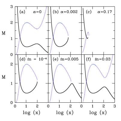
Figure 1: Variation of Mach number $M(=u/a)$ with radial distance $x$. Solid curve denotes the accretion solution and dotted curve represent the corresponding wind solution. See text for details.

In Fig. 1, we investigate the variation of Mach number ($M$) of the flow as function of logarithmic radial distance. In the upper panel, we examine the effect of viscosity ($\alpha$) on the transonic accretion solution, while in the lower panel, effect of accretion rate (${\dot{m}}$) is studied. In Fig. 1a, we choose the input parameters of the flow at the inner critical point as $x_{\rm in}=2.784$, $\lambda(x_{\rm in})=1.543$ (hereafter, $\lambda_{\rm in}$), $T_{e}(x_{\rm in})=8.7\times 10^{9}{\rm K}$ (hereafter, $T_{\rm e,~{}in}$), $\alpha=0$, and ${\dot{m}}=0.005$, respectively. In this work, although we intend to focus only on the accretion solutions, in Fig. 1, we illustrate both accretion (solid curve) and its corresponding wind branch (doted) for the purpose of completeness. In the invicid limit, the sub-sonic flow at the outer edge gains its radial velocity and subsequently becomes supersonic after crossing the inner critical point before falling in to the black hole. Solutions of this kind was studied earlier by Narayan & Yi (1995); Manmoto, Mineshige & Kusunose (1997); Rajesh & Mukhopadhyay (2010). In panel (b) and (c), viscosity is increased further and the accretion solution becomes closed and it fails to connect the horizon with the outer edge of the disc. This essentially indicates that there exists a limiting viscosity that changes the character of the accretion solutions from open to close one. The accretion solution of this kind may join with another solution that passes through the outer critical point provided a shock is formed (this will be discussed in the subsequent section) and finally merges with the Keplerian disc at the outer edge. When the viscosity is increased further, the closed topology having same inner critical point properties shrinks gradually and finally disappears. Therefore, when a global accretion flow possesses multiple critical points, there exists two critical $\alpha$ corresponding to a given set of flow parameters, where multiple critical points induct with the lower critical value of $\alpha$ and then multiple critical points disappear for the higher critical $\alpha$.

In the lower panel of Fig. 1, we demonstrate the variation of accretion solutions with accretion rate (${\dot{m}}$). For a very low accretion rate, we get a closed accretion solution shown in Fig. 1d. In this case, we choose the input flow parameters same as in Fig. 1a except the viscosity as $\alpha=0.001$. We have already pointed out above that this kind of solutions do not represent accretion solution unless they are connected with another solutions passing through the outer critical point via shock waves. When the accretion rate is increased as ${\dot{m}}=0.005$ keeping the input parameters of the flow unchanged, shock free Bondi-type accretion solution is obtained which is shown in Fig. 1e. With the continuous increase of the accretion rate, accretion solution monotonically opens up further as depicted in Fig. 1f. Note that there exists a critical accretion rate that separates the closed accretion solutions from the open accretion solutions (similar to Bondi-type). Obviously, this critical ${\dot{m}}$ is not universal, instead depends on the input parameters of the flow.

3.2 Accretion solutions with fixed outer edge

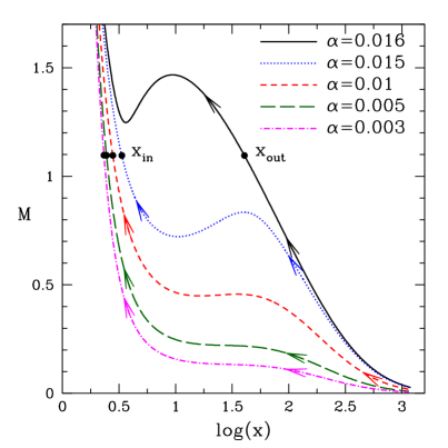
Figure 2: Variation of Mach number $M(=u/a)$ with radial distance $x$ for accretion flows injected from a fixed outer edge having different viscosity ($\alpha$). Results depicted using dot-dashed, long-dashed, dashed, dotted and solid curves are for $\alpha=0.003,0.005,0.01,0.015$ and $0.016$ respectively. Inner and outer critical points are marked in the figure as $x_{\rm in}$ and $x_{\rm out}$. See text for details.

During accretion, sub-Keplerian matter deviates from the Keplerian disc at a large distance and starts accreting towards the black hole subsonically. In accordance to this accretion scenario, it is worthy to study the dynamical properties of the accreting matter by fixing the initial conditions of the flow at the outer edge of the disc ($x_{\rm edge}$). Accordingly, for representation, we choose $x_{\rm edge}=1200$ and investigate the characteristics of the accretion solution in terms of the flow parameters fixed at $x_{\rm edge}$. We proceed to select the flow parameters at $x_{\rm edge}$ in the following manner. As before, we consider the input parameters of the flow at the inner critical point as $x_{\rm in}=2.329$, $\lambda_{\rm in}=1.719$, $T_{\rm e,~{}in}=1.789\times 10^{10}{\rm K}$, $\alpha=0.003$, and ${\dot{m}}=0.001$, respectively. Using these parameter values, we integrate equations (18-23) first inward up to horizon and then outward upto $x_{\rm edge}=1200$. Subsequently, we join these two parts of the solution to get a complete transonic global accretion solution which is denoted by the dot-dashed curve (magenta) in Fig. 2. Here, we note the flow variables at $x_{\rm edge}$ which are obtain as $u_{\rm edge}=1.56\times 10^{-4}$, $a_{\rm edge}=2.798\times 10^{-2}$, $\lambda_{\rm edge}=18.827$ and $T_{\rm e,~{}edge}=4.074\times 10^{9}{\rm K}$, respectively. Moreover, employing these local flow variables, we calculate the local energy of the flow at $x_{\rm edge}$ as ${\cal E}_{\rm edge}=2.057\times 10^{-3}$ by utilizing the expression of local energy as given by ${\cal E}(x)=0.5u^{2}+\gamma_{i}a^{2}/(\gamma_{i}-1)+0.5\lambda^{2}/x^{2}-0.5/(x-1)$. In reality, upon integrating equations (18-23) using these outer edge flow variables, one can get the same solution. Here, arrows indicate the direction of the flow towards the black hole. Next, we increase viscosity as $\alpha=0.005$ keeping $\lambda_{\rm edge}$, ${\cal E}_{\rm edge}$, $T_{\rm e,~{}edge}$ and ${\dot{m}}$ fixed at $x_{\rm edge}=1200$ and obtain another global accretion solution by suitably adjusting the values of $u_{\rm edge}=2.58\times 10^{-4}$ and $a_{\rm edge}=2.800\times 10^{-2}$ that enters into the black hole after passing through the inner critical point at $x_{\rm in}=2.4515$. In this case, the additional information of $u_{\rm edge}$ and $a_{\rm edge}$ is required to obtain the accretion solution as the critical point is not known apriori. In Fig. 2, we plot this solution using long-dashed (green) curve. Upon increasing the viscosity ($\alpha$) gradually, we identify the maximum value of viscosity as $\alpha^{\rm max}=0.015$, above this value accretion flow fails to pass through the inner critical point which is indicated by the dotted (blue) curve. The obtained results as respectively depicted by dot-dashed, long-dashed, dashed and dotted curves correspond to the solutions of advection dominated accretion flow (Narayan & Yi, 1995; Manmoto, Mineshige & Kusunose, 1997; Rajesh & Mukhopadhyay, 2010). When $\alpha$ is increased further as $0.016$, we find that the accretion solution passes through the outer critical point ($x_{\rm out}=40.594$) instead of the inner critical point ($x_{\rm in}$) which is shown by the solid (black) curve. To our knowledge, in the context of two-temperature accretion flow, self-consistent accretion solutions of this kind are not studied so far. Interestingly, accretion flows that become transonic after passing through the outer critical point ($x_{\rm out}$) are specially portentous as they may contain centrifugally supported shock waves (see §3.3).

3.3 Procedure of calculating shock locations

In an accretion flow, the inflowing matter containing multiple critical points experiences the discontinuous transition of flow variables in the form of shock waves when the Rankine-Hugoniot standing shock conditions are satisfied (Landau & Lifshitz, 1959). These conditions essentially describe the state of the accretion flow on both sides of the shock wave. At the shock front, these conditions are expressed as (a) Conservation of mass flux: $\dot{m}_{+}=\dot{m}_{-}$, (b) Conservation of energy flux: ${\cal E}_{+}={\cal E}_{-}$ and (c) Conservation of momentum: $W_{+}+\Sigma_{+}u^{2}_{+}=W_{-}+\Sigma_{-}u^{2}_{-}$, where, all the quantities have their usual meaning and ‘$-$’ and ‘$+$’ denote the quantities measured immediately before and after the shock transition. It is to be noted that in this study, we consider the shock to be thin, steady and non-dissipative in nature.

When the accretion flow possesses shock wave, inflowing matter experiences compression while crossing the shock front. In a two temperature accretion flow, such compression arises primarily due to ions only because of their higher inertia compared to the electrons. Due to compression, as ions are slowed down, kinetic energy of the ions is converted into thermal energy and electrons are expected to get a part of this thermal energy via Coulomb coupling. However, in reality, the relaxation time for electron-ion collision ($t_{\text{ei}}$) is generally higher than both the electron-electron ($t_{\text{ee}}$) and ion-ion ($t_{\text{ii}}$) collision time scales (Colpi, Maraschi & Treves, 1984; Frank, King & Raine, 2002). Hence, electron temperature is expected to be mostly unaffected across the shock front due to the shock transition. With this consideration, in this work, we assume $T_{e+}=T_{e-}$, immediately just before and after the shock.

In an accretion disc, sub-Keplerian flow starts it journey towards the black hole with almost negligible radial velocity after deviating from the Keplerian disc (Chakrabarti, 1990). Due to the gravitational attraction, flow gains it radial velocity and becomes supersonic after crossing the outer critical point ($x_{\rm out}$). Flow continues to move further before jumping to the sub-sonic branch via shock transition and subsequently crosses the inner critical point ($x_{\rm in}$) before falling in to the black hole. In order to obtain such a global accretion solution including shock wave, for computational simplicity, we begin our numerical integration of equations (18,21,22,23) from $x_{\rm out}$ and continue once outward up to $x_{\rm edge}$ for subsonic branch and then inward towards the black hole horizon for the supersonic branch. While calculating the supersonic branch, we search for the shock location and associated inner critical point in the following way. Using a set of supersonic local flow variables, namely $x$, $u$, $a$, $M$ and $\rho$, we calculate the total pressure and local energy of the flow. Since these quantities along with the accretion rate, specific angular momentum and electron temperature remain conserved across the shock front, we employ these conserved quantities to calculate the same set of local flow variables for the subsonic branch (Chakrabarti & Das, 2004). Employing these subsonic local flow variables, we continue integration towards the black hole horizon to find an inner critical point ($x_{\rm in}$) where $N$ and $D$ of equation (18) tend to zero simultaneously. Upon failing to obtain the inner critical point, we choose another set of supersonic local flow variables by decreasing $x$ and again look for $x_{\rm in}$. We continue the process and once $x_{\rm in}$ is found, the shock location ($x_{s}$) is obtained as $x_{s}=x$. Needless to mention that the obtained $x_{\rm in}$ represents an unique location corresponding to a given set of input flow parameters including $x_{\rm out}$. Using the inner critical point flow variables, we again carry out the numerical integration further and continue up to the inner edge of the disc. With this, eventually we obtain a global accretion solution that passes through two saddle type critical point (namely, $x_{\rm in}$ and $x_{\rm out}$) and these points are connected through the shock wave located at $x_{s}$. What is more is that following the above procedure, we uniquely determine the shock location for a given set of input parameters chosen at the outer critical point ($x_{\rm out}$). Conversely, one can repeat the same exercise choosing the flow parameters at the inner critical point ($x_{\rm in}$) as well while calculating the location of shock transition.

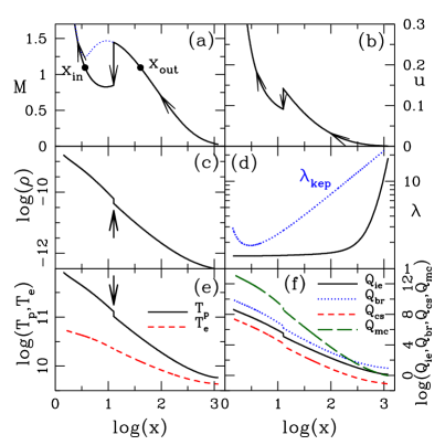
Figure 3: Variation of (a) Mach number $M(=u/a)$, (b) radial velocity ($u$), (c) density ($\rho$), (d) angular momentum ($\lambda$), (e) electron and ion temperature ($T_{e},T_{i}$), and (f) cooling rates of the accretion flow as a function of radial distance. The shock solution presented here corresponds to result depicted by solid (black) curve in Fig. 2. See text for details.

3.4 Accretion solutions containing shock

In Fig. 3a, we demonstrate the shock induced global accretion solution corresponding to the result depicted using solid curve (black) in Fig. 2. Here, inflowing matter changes its sonic state after crossing the outer critical point ($x_{\rm out}=40.594$) to become super-sonic and continues to accrete towards the black hole. In principle, such supersonic matter can smoothly enter into the black hole as indicated by the dotted curve (Fig. 3a). However, we observe that the supersonic matter has the potential to join with the subsonic branch passing through the inner critical point ($x_{\rm in}=3.6529$) having $\lambda_{\rm in}=1.3947$ and $T_{\rm e,in}=4.074\times 10^{10}{\rm K}$ through a shock transition. We find that the shock conditions are favourable in both the pre-shock and post-shock flow and these conditions are satisfied at $x_{\rm s}=12.6370$, where the supersonic flow encounters a discontinuous transitions of its variables to the subsonic branch. In the figure, inner critical point ($x_{\rm in}$) and the outer critical point ($x_{\rm out}$) are marked and the solid vertical arrow indicates the shock jump. In Fig. 3b, we present the variation of radial velocity corresponding the solution presented in Fig. 3a. Discontinuous transition of radial velocity from supersonic to subsonic value is indicated by the vertical arrow. As before, the direction of the arrows shows the direction of the flow motion towards the black hole. According to the second law of thermodynamics, nature favors those accretion solutions that have high entropy content (Becker & Kazanas, 2001). Incidentally, the supersonic inflowing matter passing through outer critical point possesses less entropy than the subsonic inflowing matter passing through inner critical point. Hence, supersonic inflowing matter prefers to follow the subsonic branch of the solution while falling towards the black hole and this happens through the discontinuous shock transition. In Fig. 3c, we present the variation of density profile as function of radial distance. We observe the compression of the inflowing matter in the post-shock region as density jumps sharply across the shock. This is shown by the solid curve where vertical arrow indicates density enhancement at shock. This happens mainly due to the reduction of radial velocity in the post-shock region. In Fig. 3d, we show the radial variation of angular momentum for the same solution as shown in Fig. 3a and it is denoted by the solid curve. We also depict the Keplerian angular momentum distribution in the plot which is shown by the dotted curve (blue). The adopted viscosity prescription confirms the continuity of the angular momentum distribution across the shock. We continue our investigation of disc structure and in Fig. 3e, we show the temperature distribution of ion (obtained using sound speed) and electron for the same solution as depicted in Fig. 3a, where solid and dashed curves represent the results for ions and electrons, respectively. Here, the collisional energy transfer between ions and electrons is largely inefficient and the cooling time scale of the fast moving electrons are shorter than the slowly moving ions. These considerations permit the inflowing matter to maintain two temperature distribution. In addition to that ion temperature shoots up discontinuously in the post shock region due to shock compression which is denoted by the solid vertical arrow. The electron temperature remain unaffected across the shock as we consider that the relaxation time for $e-i$ collision ($t_{\text{ei}}$) is large compared to the $e-e$ and $i-i$ collision time scales (Colpi, Maraschi & Treves, 1984; Frank, King & Raine, 2002). For instance, we calculate the ratio of time scales across the shock front which are obtained as $t_{\rm ei}/t_{\rm ee}\sim 920$ and $t_{\rm ii}/t_{\rm ee}\sim 425$, respectively. Fig. 3f shows the energy dissipation rates per unit volume resulting from the Coulomb coupling, bremsstrahlung process, synchrotron process and inverse Comptonization of synchrotron photons, respectively. Solid, dotted, dashed and long-dashed curves denote the radial variation of coulomb coupling $(Q_{ie})$, bremsstrahlung cooling rate $(Q_{br})$, synchrotron cooling rate $(Q_{cs})$, and Comptonization due to synchrotron photon $(Q_{mc})$. In the post-shock region all these cooling terms increases efficiently due to increase of density across the shock transition.

Figure 4: Variation of Mach number $M(=u/a)$ with radial distance $x$ for accretion flows injected with various accretion rate (${\dot{m}}$) from the outer edge of the disc. Solutions plotted with dashed, dotted and solid curves are for ${\dot{m}}=10^{-4},0.1$ and $0.2$, respectively. See text for details.

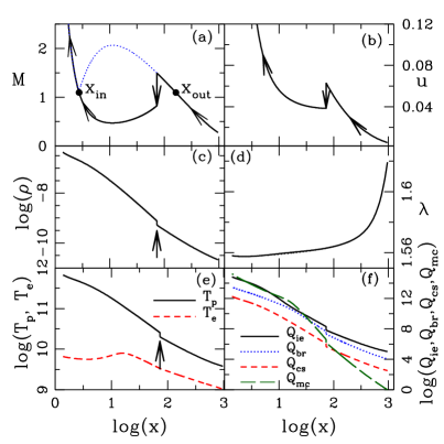
Figure 5: Variation of (a) Mach number $M(=u/a)$, (b) radial velocity ($u$), (c) density ($\rho$), (d) angular momentum ($\lambda$), (e) electron and ion temperature ($T_{e},T_{i}$), and (f) cooling rates as a function of radial distance. This shock solution corresponds to solid (black) curve in Fig. 4. See text for details.

In §3.2, we have shown how the flow characteristics are altered when viscosity is increased for flows having boundary conditions fixed at the outer edge of the disc. In a similar way, here we continue our investigation while making an attempt to examine the role of accretion rate in deciding the characteristic of the accretion flow. Towards this, we choose the outer boundary of the disc as $x_{\rm edge}=1000$, $\lambda_{\rm edge}=1.6257$, $T_{\rm e,~{}edge}=1\times 10^{9}{\rm K}$, ${\cal E}_{\rm edge}=6.197\times 10^{-4}$, ${\dot{m}}=10^{-4}$ and $\alpha=0.001$, respectively and obtain the global accretion solution passing through the inner critical point as $x_{\rm in}=2.7517$ before falling into the black hole. The result is depicted in Fig. 4, where Mach number ($M$) is plotted as function of radial coordinate. In the figure, the dashed curve denotes the accretion solution corresponding to ${\dot{m}}=10^{-4}$. Next, we increase the accretion rate as ${\dot{m}}=0.1$ keeping the remaining flow parameters fixed at $x_{\rm edge}$ and get the accretion solution analogous to the result obtained for ${\dot{m}}=10^{-4}$. This result is depicted using dotted curve in Fig. 4. When the accretion rate is increased further as ${\dot{m}}=0.2$, inflowing matter changes its character as it passes through the outer critical point ($x_{\rm out}=162.837$) instead of inner critical point and the result is shown by the solid curve. After crossing $x_{\rm out}$, accretion flow becomes supersonic and continues to proceed towards the black hole. Eventually, centrifugal repulsion turns out to be comparable against gravity that renders the triggering of the discontinuous transition of flow variables in the form of shock wave. In Fig. 5, we present the radial variation of Mach number ($M$), radial velocity ($u$), density ($\rho$), angular momentum ($\lambda$), temperatures ($T_{e},T_{i}$) and various cooling rates ($Q_{ie},Q_{br},Q_{cs},Q_{mc}$) including shock transition for ${\dot{m}}=0.2$. The general behavior of the above mentioned flow variables with radial coordinate are very much similar to the results presented in Fig. 3 and therefore, here we skip their description to avoid repetition although Fig. 3f and Fig. 5f indicates that the contributions from the different cooling heads are strongly depended on the accretion rate which is indeed firmly expected.

3.5 Shock Dynamics and Shock Properties

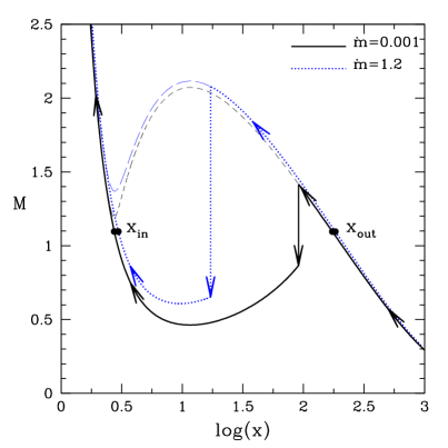
Figure 6: Plot of global accretion solutions including shock waves. Flows with fixed outed boundary parameters are injected with different accretion rates (${\dot{m}}$ which are marked in the figure. Each solution contains shock waves which are shown by the vertical arrow as $x_{s}=91.107$ (solid) and $x_{s}=16.757$ (dotted). See text for details.

In the course of shock study, it is customary to explore the influence of the global flow parameters, namely accretion rate (${\dot{m}}$) and viscosity ($\alpha$), on the dynamical behavior of shock waves. Hence, as an example, we first choose an accretion flow having outer boundary parameters as $x_{\rm edge}=1000$, $\lambda_{\rm edge}=1.844$, $T_{\rm e,~{}edge}=2\times 10^{9}{\rm K}$, ${\cal E}_{\rm edge}=5.322\times 10^{-4}$ and $\alpha=0.005$, respectively and vary the accretion rate (${\dot{m}}$). When ${\dot{m}}=0.001$ is considered, we find that flow encounters stationary shock transition at $x_{s}=91.107$. This result is depicted in Fig. 6, where the variation of Mach number is plotted as function of radial coordinate. In the figure, solid curve denotes the shock induced global accretion solution corresponding to ${\dot{m}}=0.001$. Moreover, the solid vertical arrow indicates the location of shock transition and $x_{\rm in}$ and $x_{\rm out}$ denote the inner and outer critical points. Overall, arrows indicate the direction of flow motion towards the black hole. As ${\dot{m}}$ is increased, the effective radiative cooling efficiency in the post-shock region is enhanced that reduces the post-shock pressure. Eventually, shock front moves inward in order to maintain the pressure balance across the shock. Accordingly, we identify the maximum value of the accretion rate as $\dot{m}^{\rm max}=1.2$ that allows the flow to pass through the stationary shock transition. Needless to mention that $\dot{m}^{\rm max}$ does not possess the universal value, instead it strongly depends on the other flow parameters. For this accretion rate ($\dot{m}^{\rm max}=1.2$), we calculate the global accretion solution including shock and plot it using dotted curve in Fig. 6. As before, vertical dotted arrow indicates the shock location at $x_{s}=16.787$. When $\dot{m}>\dot{m}^{\rm max}$, accretion solution including standing shock ceases to exist. However, non-steady shock may still continue to present in the flow which could exhibit the time dependent physical processes similar to quasi-periodic oscillations (QPOs) as frequently observed in the case of Galactic black hole sources. Unfortunately, the study of such scenarios are beyond the scope of the present paper. We plan to consider the numerical investigation as a future project and will be reported elsewhere.

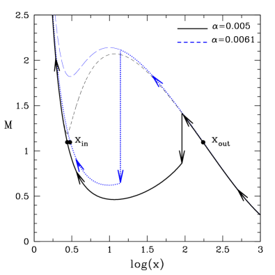
Figure 7: Same as Fig. 6, but the accretion solutions are obtained for different viscosity ($\alpha$) which are marked in the figure. Each solution contains shock waves which are shown by the vertical arrow as $x_{s}=91.107$ (solid) and $x_{s}=13.969$ (dotted). See text for details.

In the subsequent analysis, we examine the role of viscosity ($\alpha$) in deciding the formation of stationary shock in an accretion flow having fixed outer boundary conditions. As in the case of Fig. 6, here again we consider the accretion flow having outer boundary conditions as $x_{\rm edge}=1000$, $\lambda_{\rm edge}=1.844$, $T_{\rm e,~{}edge}=2\times 10^{9}{\rm K}$, ${\cal E}_{\rm edge}=5.322\times 10^{-4}$, ${\dot{m}}=0.001$ and vary $\alpha$ to obtain the shock induced global accretion solutions. When viscosity is chosen as $\alpha=0.005$, we find that flow encounters standing shock transition at $x_{s}=91.107$ which is denoted by the solid vertical arrow in Fig. 7. Here again, arrows indicate the direction of the flow motion during the course of accretion on to the black hole. In addition, inner and outer critical points are indicated in the figure as $x_{\rm in}$ and $x_{\rm out}$, respectively. When viscosity is increased, angular momentum of the flow is being transported outwards more rapidly that causes the weakening of centrifugal repulsion against gravity. As a consequence, shock front settles down at a smaller radial coordinate just to maintain the pressure balance across the shock. We calculate the minimum shock location ($x_{s}^{\rm min}$) by increasing the $\alpha$ and find $x_{s}^{\rm min}=13.969$ for $\alpha=0.0061$. Obviously, the obtained $x_{s}^{\rm min}$ depends on the other flow variables that we keep fixed here at the outer edge of the disc. In the figure, we indicate the shock transition corresponding to $\alpha=0.0061$ by the dotted vertical arrow. When $\alpha>0.0061$, standing shock conditions are not favorable, and therefore, stationary shock disappears.

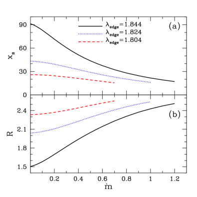
Figure 8: Variation of (a) shock location ($x_{s}$) and (b) compression ratio ($R$) with accretion rate $(\dot{m})$ for flows with fixed outer boundary parameters. Solid, dotted and dashed curves are for $1.844$, $1.824$ and $1.804$ respectively. See text for details.

In Fig. 8, we investigate the shock properties as function of accretion rate ${\dot{m}}$. Here, we choose the outer edge of the disc at $x_{\rm edge}=1000$ and inject matter with ${\cal E}_{\rm edge}=5.322\times 10^{-4}$, $T_{\rm e,edge}=2\times 10^{9}{\rm K}$ and $\alpha=0.005$. In the upper panel (Fig. 8a), we show the variation of shock location corresponding to the different $\lambda_{\rm edge}$. The solid, dotted and dashed curves are for $\lambda_{\rm edge}=1.844$, $1.824$ and $1.804$, respectively. For a given $\lambda_{\rm edge}$, as illustrated in the figure, shock front proceeds towards the black hole horizon with the increase of accretion rate (${\dot{m}}$) irrespective to the angular momentum at the outer edge. Evidently, it is not possible to get the shocked accretion solution when ${\dot{m}}$ is exceedingly large. This is because there exists a maximum value of accretion rate (${\dot{m}^{\rm max}}$ ) corresponding to the chosen outer boundary flow parameters. When ${\dot{m}}>{\dot{m}^{\rm max}}$, the possibility of shock formation fails as shock conditions are not satisfied there. Moreover, for a given ${\dot{m}}$ we find the shock to form further out for flows with higher $\lambda_{\rm edge}$. This establishes the fact that the possibility of shock transition is perhaps centrifugally driven. Meanwhile, we have pointed out in the Fig. (3) and Fig. (5) that density is enhanced in the post-shock region due to shock compression. Since the radiative cooling processes largely depend on the matter density, emergent radiations from the disc are also rely upon it and therefore, it is worthy to examine the density jump of the flow across the shock. Accordingly, we calculate the density compression of the flow across the shock by computing the compression ratio which is defined as the ratio of vertically averaged post-shock and the pre-shock density ($R=\Sigma_{+}/\Sigma_{-}$). In Fig. 8b, we present the variation of the compression ratio ($R$) with ${\dot{m}}$ for the same set of flow parameters as used in Fig. 8a. With the increase of ${\dot{m}}$, as the shock front proceeds towards the black hole horizon, post-shock flow experiences further compression and hence, $R$ increases with the increase of ${\dot{m}}$.

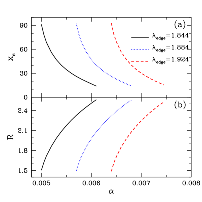
Figure 9: Variation of (a) shock location ($x_{s}$) and (b) compression ratio ($R$) as function of viscosity ($\alpha$) for flows injected with fixed outer boundary parameters. Solid, dotted and dashed curves are for $\lambda_{\rm edge}=1.844,1.884$ and $1.924$, respectively. See text for details.

In the next, we carry out the investigation of shock properties by varying viscosity $\alpha$ for flows with fixed outer boundary conditions. The obtained results are presented in Fig. 9 where we choose $x_{\rm edge}=1000$, ${\cal E}_{\rm edge}=5.322\times 10^{-4}$, $T_{\rm e,edge}=2\times 10^{9}{\rm K}$ and ${\dot{m}}=0.001$, respectively. Here, solid, dotted and dashed curves represented the results corresponding to $\lambda_{\rm edge}=1.844$, $1.884$ and $1.924$, respectively. As illustrated in Fig. 9a, shock front proceeds towards the black hole horizon with the increase of $\alpha$ irrespective to the angular momentum at the outer edge. For a given $\lambda_{\rm edge}$, when $\alpha$ is increased, $\lambda(x)$ is decreased along the flow motion. This weakens the centrifugal repulsion against the gravity and causes the shock front to move inward. Moreover, for a fixed $\alpha$, shock forms at a larger distance from the horizon when $\lambda_{\rm edge}$ is increased. This happens because large $\lambda_{\rm edge}$ increases the strength of the centrifugal barrier and therefore, the shock front is pushed outside. This findings again clearly indicates that the centrifugal force eventually plays the pivotal role in deciding the formation of shock wave in an accretion disc. In addition, there exists a limiting range of $\alpha$ associated to a given outer boundary conditions of the flow. Out side this range of $\alpha$, standing shock conditions are not favorable and therefore, global accretion solution including shock wave ceases to exist. As before, we calculate the compression ratio ($R$) across the shock front corresponding to the shocked accretion solution depicted in Fig. 9a. We plot the obtained results in Fig. 9b where we observe positive correlation between $R$ and $\alpha$.

4 Shock Parameter Space

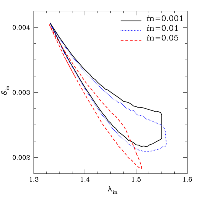
Figure 10: Plot of $\lambda_{\rm in}-{\cal E}_{\rm in}$ parameter space for shock. Region bounded by solid, dotted and dashed curves for ${\dot{m}}=0.001,0.01$ and $0.05$, respectively. As ${\dot{m}}$ is enhanced, parameter space is shifted to lower energy side due to energy dissipation in the form of radiative cooling. See text for details.

It is already observed that the two-temperature transonic accretion flows around black holes possess shock waves and accretion solutions of this kind are not the discrete solutions, in fact they exist for a wide range of flow parameters. To validate this claim and also to understand the influence of flow parameters on the shock induced global accretion solutions, we separate the regions of parameter space spanned by the angular momentum ($\lambda_{\rm in}$, measured at $x_{\rm in}$) and the local energy of the flow (${\cal E}_{\rm in}$, measured at $x_{\rm in}$) that allows shocked accretion solutions. We calculate the shock parameter space at $x_{\rm in}$ due to the fact that the acceptable range of the angular momentum at the inner edge of the disc and the location of the inner critical points are $1.2\lesssim\lambda_{\rm in}\lesssim 2$ and $2\lesssim x_{\rm in}\lesssim 4$, respectively (Chakrabarti, 1990; Chakrabarti & Das, 2004). Therefore, we can safely assume that the flow enters in to the black hole with angular momentum and energy similar to their values measured at $x_{\rm in}$. In Fig. 10, we present the classification of shock parameter space in terms of the accretion rate (${\dot{m}}$). The region bounded by the solid, dotted and dashed curves are obtained for ${\dot{m}}=0.001,0.01$ and $0.05$, respectively. Here, we choose $\alpha=0.01$ and $T_{\rm e,in}=6.75\times 10^{9}{\rm K}$. As ${\dot{m}}$ is increased, the effective region of the parameter space for shock is shrunk. When the adopted cooling processes are active in the flow, inflowing matter loses its energy while accreting towards the black hole. This eventually causes the parameter space to shift in the lower energy domain for increasing accretion rate of the flow. Moreover, when ${\dot{m}}$ gradually increases, beyond its critical limit, the parameter space disappears completely as standing shock conditions fail to satisfy there.

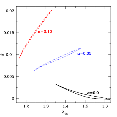
Figure 11: Plot of $\lambda_{\rm in}-{\cal E}_{\rm in}$ parameter space for shock. Region bounded by different line styles are for different viscosity parameter ($\alpha$). The lowermost parameter space is drawn for $\alpha=0$. As $\alpha$ is increased ($\Delta\alpha=0.05$) which are marked in the plot, shock parameter space is shifted to higher energy and lower angular momentum domain. See text for details.

We continue our investigation to study the variation of the shock parameter space for flows with varying viscosity parameters ($\alpha$) and present the results in Fig. 11, where the shock parameter space corresponding to a given viscosity parameter is marked. Here, we choose ${\dot{m}}=0.05$ and $T_{\rm e,in}=6.75\times 10^{9}{\rm K}$, respectively. We observe that shock parameter space is shifted towards the lower angular momentum and higher energy domain when $\alpha$ is increased. This is the consequence of the dual effects of viscosity in an accretion flow where viscosity not only transports the angular momentum outwards, but also dissipates energy as well. Moreover, we observed that standing shocks can form even for a low angular momentum flows provided the viscosity is chosen to be sufficiently large. However, it is not possible to increase the viscosity indefinitely. This is because above a critical viscosity limit, standing shock transition in an accretion flow does not occur and consequently, shock parameter space disappears. It is to be noted that the value of the critical viscosity is not universal, instead it largely depends on the other parameters of the flow.

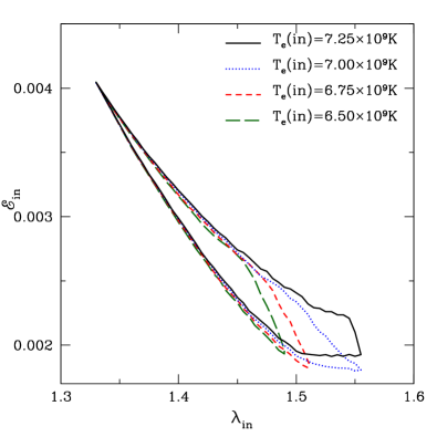
Figure 12: Modification of $\lambda_{\rm in}-{\cal E}_{\rm in}$ shock parameter space as function of $T_{\rm e,in}$. $T_{\rm e,in}$ values are marked in the figure that denote parameter spaces separated with different line styles. See text for details.

We further classify the shock parameter space as function of $T_{\rm e,in}$ and present the results in Fig. 12. Here, we choose ${\dot{m}}=0.05$ and $\alpha=0.01$, respectively. The shock parameter spaces are separated using boundaries drawn with long-dashed, dashed, dotted and solid curves which are obtained for $T_{\rm e,in}=6.50\times 10^{9}{\rm K},6.75\times 10^{9}{\rm K},7.00\times 10^{9}{\rm K}$ and $7.25\times 10^{9}{\rm K}$, respectively. We find that the effective region of the shock parameter space is reduced with the decrease of $T_{\rm e,in}$. This is not surprising because in order to obtain an accretion solution having smaller $T_{\rm e,in}$, the overall cooling efficiency needs to be higher and the increasing cooling effect reduces the effective region of the parameter space for standing shock (see Fig. 10). In addition, Fig. 12 clearly indicates that there exists a range of $T_{\rm e,in}$ which allows standing shock transition for a given set of input parameters of the flow.

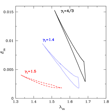
Figure 13: Modification of parameter space for standing shock as function of ions specific heats ratio ($\gamma_{i}$). Parameter spaces bounded with solid, dotted and dashed curves are for $\gamma_{i}=4/3,1.4$ and $1.5$, respectively. See text for details.

In a two-temperature accretion flow, since electrons are lighter than the protons, it is customary to treat electrons as relativistic in nature while protons are considered as non-relativistic. Accordingly, as a conservative estimate, so far we have chosen the adiabatic indices for electrons and ions as $\gamma_{e}=4/3$ and $\gamma_{i}=3/2$, respectively. However, in a realistic scenario, $\gamma_{i}$ is expected to vary depending on the ratio between the thermal energy and the rest mass energy of the ions (Frank, King & Raine, 2002). In order to understand the effect of $\gamma_{i}$ on the two-temperature global shock solutions, we calculate the parameter space for standing shock similar to Fig. 10 for three different values of $\gamma_{i}$ and depict the result in Fig. 13, where the parameter spaces separated with solid, dotted and dashed boundary are for $\gamma_{i}=4/3,1.4$ and $1.5$, respectively. Here, we choose $\alpha=0.01$, ${\dot{m}}=0.05$ and $T_{\rm e,in}=7\times 10^{9}{\rm K}$. We find that standing shock exists in all three cases and also observe that the effective region of the parameter space for standing shock is large for lower values of $\gamma_{i}$ and it reduces considerably when ions changes its character towards the non-relativistic limit.

5 Conclusions

In this paper, we provide a self-consistent formalism to study the properties of a two-temperature accreting flow around a Schwarzschild black hole. We choose the inflowing matter to be rotating, viscous and advection dominated which is confined within a thin disc structure. Radiative processes, namely, bremsstrahlung, cyclo-synchrotron and Comptonization of synchrotron photons processes are considered to be active in the flow. Moreover, we consider that the interaction between electrons and ions is guided by the Coulomb coupling process. During the course of accretion towards the black hole, rotating matter experiences centrifugal repulsion that eventually triggers the discontinuous transition of flow variables in the form of shock waves. Based on the consideration of second law of thermodynamics, shock induced two-temperature global accretion solutions around black holes are thermodynamically preferred over the smooth solutions as the former possess high entropy content (Becker & Kazanas, 2001). With this, for the first time to our knowledge, we obtain the self-consistent two-temperature global accretion solutions including shock waves by solving the coupled hydrodynamic equations for ions and electrons simultaneously. These shocked accretion solutions seem to be essential to understand the observed spectral and timing properties of the black hole candidates (Chakrabarti & Manickam, 2000; Nandi et al., 2001a, b, 2012; Radhika & Nandi, 2014; Iyer, Nandi & Mandal, 2015; Radhika et al., 2016a, b).

We obtain the two-temperature global accretion solutions containing shock waves in presence of dissipation processes, namely, radiative coolings and viscosity (Fig. 3 and Fig. 5). We observe that due to the discontinuous shock transition, post-shock flow (equivalently PSC) is compressed that causes the PSC to become hot and dense. Incidentally, synchrotron and bremsstrahlung photons in PSC are likely to be reprocessed via inverse Comptonozation to produce hard radiations (Chakrabarti & Titarchuk, 1995; Mandal & Chakrabarti, 2005) which are commonly observed from the accretion systems harboring black hole candidates. This clearly gives a hint that the size of the PSC ($i.e.$, shock location, $x_{s}$) perhaps play key role in emitting the high energy photons from the disc. Moreover, for an accretion flow injected from a fixed outer edge, we find that the dynamics of the shock front is regulated by the dissipation parameters. When accretion rate (${\dot{m}}$) is increased, the effect of cooling becomes more efficient in the post-shock flow resulting the reduction of thermal pressure at PSC. In order to maintain the balance of total pressure across the shock front, PSC is forced to settle down to a smaller radius from the black hole (Fig. 6). Similarly, as the viscosity ($\alpha$) is increased, the efficiency of angular momentum transport in the outward direction is enhanced causing the weakening of centrifugal repulsion against gravity. This eventually compels the shock front to move towards the black hole just to maintain pressure balance across the shock front (Fig. 7). Overall, in our two-temperature model, we find that shock induced global accretion solutions are not isolated solutions as shock exists for a wide range of dissipation parameters. Interestingly, when dissipation parameters exceed there critical limits for flows with fixed injection boundary, PSC disappears as the standing shock conditions fail to satisfy for a highly dissipative flow (Fig. 8-9).

One of the motivation of this work is to identify the ranges of flow parameters that allow shock in two-temperature accretion flow. In Fig. 10, we explore the parameter space within which the two-temperature accretion flow with shock can exist as function of angular momentum and energy both measured at the inner critical point for various values of accretion rate (${\dot{m}}$). As ${\dot{m}}$ is increased, dissipation due to cooling is increased and flow loses its energy while advecting towards the black hole. This reduces the possibility of shock formation and effectively the shock parameter space is shrunk and shifted towards the lower energy side. Further, we separate the parameter space for shock as function of viscosity ($\alpha$) as well and find that shock region is reduced and displaced towards the higher energy and lower angular momentum domain as $\alpha$ is increased (Fig. 11). This happens due to the dual role of viscosity as the increase of $\alpha$ enhances the outward diffusion of angular momentum and also dissipates energy in the flow. Moreover, we calculate the shock parameter space as function of electron temperature at the inner critical point ($T_{\rm e,in}$) and find the the effective region of the shock parameter space is reduced with the decrease of $T_{\rm e,in}$ (Fig.12).

Since ions are more massive than electrons, in this work, we treat ions as thermally non-relativistic and consider the adiabatic index for ions in most of cases as $\gamma_{i}=3/2$. However, in reality, the theoretical limit of $\gamma_{i}$ lies in the range between $4/3$ to $5/3$ depending on the ratio between the thermal energy and the rest mass energy of the ions (Frank, King & Raine, 2002). To infer this, we calculate the shock parameter space for three different $\gamma_{i}$ and observe that global shock solutions exist in all cases. Moreover, we find that shock parameter space is shrunk as $\gamma_{i}$ is increased which essentially indicates that possibility of shock formation is reduced for higher $\gamma_{i}$.

The self-consistent two-temperature global shocked accretion solutions have extensive implications in the context of modeling of observational features of black hole sources. In fact, these hydrodynamical shock solutions in presence of the relevant cooling mechanisms are perhaps essential to calculate the emission spectrum of a black hole system (Chakrabarti & Titarchuk, 1995; Mandal & Chakrabarti, 2005). So far, several theoretical attempts were made to examine the spectral behavior of black hole sources considering shock properties in a parametric way Mandal & Chakrabarti (2005); Chakrabarti & Mandal (2006). In order for generalization, a study of the spectral properties of black holes involving the self-consistent two-temperature shocked accretion solution is under progress and will be reported elsewhere.

Finally, we discuss the limitations of the present work as it is developed based on some approximations. We use pseudo-Newtonian gravitational potential to describe the space-time geometry around the black hole which allows us to study the non-linear shock phenomenon and its properties avoiding the complicated general relativistic calculations. Moreover, we consider the constant adiabatic indices for both ions and electrons instead of estimating them self-consistently based on the thermal properties of the flow (Ryu, Chattopadhyay & Choi, 2006; Kumar et al., 2013; Kumar & Chattopadhyay, 2014) . Further, we choose stochastic magnetic field configuration rather ignoring the large scale magnetic fields and also neglect the effects of radiation pressure. Of course, the implementation of such issues is beyond the scope of present paper. However, we believe that the basic conclusions of this work will remain qualitatively unaltered due to the above approximations.

Appendix: Calculation of radial velocity gradient at critical point

The radial velocity gradient at the critical point ($x_{c}$) has the form $(du/dx)=0/0$. Hence, in order to understand the behavior of the flow properly, we apply the l^′Hospital rule at $x_{c}$ (Kopp & Holzer, 1976; Holzer, 1977; Jacques, 1978) and therefore, obtain the expression of the radial velocity gradient at the critical point ($x_{c}$) as,

$$\left(\frac{du}{dx}\right)_{c}=\frac{N_{1}-D_{2}\pm\sqrt{(N_{1}-D_{2})^{2}+4D_{1}N_{2}}}{2D_{1}},$$

where

$$N_{1}= \Lambda_{11}-\Gamma_{21}-\frac{\frac{\lambda^{2}}{x^{3}}-F}{\gamma_{i}-1}-\frac{\gamma_{i}a}{\gamma_{i}-1}-\frac{\gamma_{i}a^{2}}{\gamma_{i}-1}\left(\frac{3}{2x}-\frac{1}{2F}\frac{dF}{dx}\right)$$

$$-\frac{u}{\gamma_{i}-1}\frac{2\lambda\lambda_{11}}{x^{3}}-\frac{\gamma_{i}au}{\gamma_{i}-1}a_{121}$$

$$-\bigg{[}\frac{\gamma_{i}u}{\gamma_{i}-1}+\frac{2\gamma_{i}au}{\gamma_{i}-1}\left(\frac{3}{2x}-\frac{1}{2F}\frac{dF}{dx}\right)\bigg{]}a_{11},$$

$$N_{2}= \Lambda_{12}-\Gamma_{22}-\frac{u}{\gamma_{i}-1}\left(\frac{2\lambda\lambda_{12}}{x^{3}}-\frac{3\lambda^{2}}{x^{4}}-\frac{dF}{dx}\right)-\frac{\gamma_{i}au}{\gamma_{i}-1}a_{122}$$

$$-\frac{\gamma_{i}a^{2}u}{\gamma_{i}-1}\left(-\frac{3}{2x^{2}}+\frac{1}{2F^{2}}\left(\frac{dF}{dx}\right)^{2}-\frac{1}{2F}\frac{d^{2}F}{dx^{2}}\right)$$

$$-\bigg{[}\frac{\gamma_{i}u}{\gamma_{i}-1}+\frac{2\gamma_{i}au}{\gamma_{i}-1}\left(\frac{3}{2x}-\frac{1}{2F}\frac{dF}{dx}\right)\bigg{]}a_{12},$$

$$D_{1}= \frac{4\gamma_{i}a}{\gamma_{i}-1}a_{11}-2\frac{\gamma_{i}+1}{\gamma_{i}-1}u+\Gamma_{11},$$

$$D_{2}= \frac{4\gamma_{i}a}{\gamma_{i}-1}a_{12}+\Gamma_{12},$$

$$\Lambda_{11}= -\left(\Lambda_{ie}+\Lambda_{ib}\right)\left(\frac{a_{11}}{a}+\frac{1}{u}\right)$$

$$+\left(\frac{\Lambda_{ie}}{T_{i}-T_{e}}+\frac{\Lambda_{ib}}{2T_{i}}\right)T_{21}-\Lambda_{ie}\left(\frac{1}{T_{i}-T_{e}}-\frac{3}{2T_{e}}\right)T_{11},$$

$$\Lambda_{12}= -(\Lambda_{ie}+\Lambda_{ib})\left(\frac{a_{12}}{a}+\frac{3}{2x}-\frac{1}{2F}\frac{dF}{dx}\right)$$

$$+\left(\frac{\Lambda_{ie}}{T_{i}-T_{e}}+\frac{\Lambda_{ib}}{2T_{i}}\right)T_{22}-\Lambda_{ie}\left(\frac{1}{T_{i}-T_{e}}-\frac{3}{2T_{e}}\right)T_{12},$$

$$\Gamma_{11}= \frac{-4\alpha I_{n}(gaa_{11}+u)\lambda_{11}}{x}-\frac{2\alpha I_{n}(ga^{2}+u^{2})\lambda_{111}}{x},$$

$$\Gamma_{12}= \frac{-4\alpha I_{n}(gaa_{12})\lambda_{11}}{x}-\frac{2\alpha I_{n}(ga^{2}+u^{2})\lambda_{112}}{x}$$

$$+\frac{2\alpha I_{n}(ga^{2}+u^{2})\lambda_{11}}{x^{2}},$$

$$\Gamma_{21}= \frac{-4\alpha I_{n}(gaa_{11}+u)\lambda_{12}}{x}-\frac{2\alpha I_{n}(ga^{2}+u^{2})\lambda_{121}}{x}$$

$$+\frac{8\alpha I_{n}(gaa_{11}+u)\lambda}{x^{2}}+\frac{4\alpha I_{n}(ga^{2}+u^{2})\lambda_{11}}{x^{2}},$$

$$\Gamma_{22}= \frac{-4\alpha I_{n}gaa_{12}\lambda_{12}}{x}-\frac{2\alpha I_{n}(ga^{2}+u^{2})\lambda_{122}}{x}$$

$$+\frac{2\alpha I_{n}(ga^{2}+u^{2})\lambda_{12}}{x^{2}}+\frac{8\alpha I_{n}gaa_{12}\lambda}{x^{2}}$$

$$+\frac{4\alpha I_{n}(ga^{2}+u^{2})\lambda_{12}}{x^{2}}-\frac{8\alpha I_{n}(ga^{2}+u^{2})\lambda}{x^{3}},$$

$$a_{111}= \left(\frac{1}{u}+\frac{u}{a^{2}}\right)a_{11}-\left(\frac{1}{a}+\frac{a}{u^{2}}\right),$$

$$a_{112}= \left(\frac{1}{u}+\frac{u}{a^{2}}\right)a_{12},$$

$$a_{121}= -\frac{1}{a^{2}}\bigg{\{}\frac{\lambda^{2}}{x^{3}}-F\bigg{\}}a_{11}+\bigg{\{}\frac{3}{2x}+\frac{1}{2F}\frac{dF}{dx}\bigg{\}}a_{11}+\frac{2\lambda\lambda_{11}}{ax^{3}},$$

$$a_{122}= -\frac{1}{a^{2}}\bigg{\{}\frac{\lambda^{2}}{x^{3}}-F\bigg{\}}a_{12}+\bigg{\{}\frac{3}{2x}+\frac{1}{2F}\frac{dF}{dx}\bigg{\}}a_{12}+\frac{2\lambda\lambda_{12}}{ax^{3}}$$

$$-\frac{1}{a}\left(\frac{3\lambda^{2}}{x^{4}}+\frac{dF}{dx}\right)+a\bigg{\{}-\frac{3}{2x^{2}}+\frac{1}{2F^{2}}\left(\frac{dF}{dx}\right)^{2}-\frac{1}{2F}\frac{d^{2}F}{dx^{2}}\bigg{\}},$$

$$\lambda_{111}= \frac{\alpha(ga^{2}-u^{2})}{u^{3}}-\frac{2\alpha(gaa_{11}-u)}{u^{2}}$$

$$+\frac{2\alpha gaxa_{11}}{u}\left(\frac{a_{11}}{a}-\frac{1}{u}+\frac{a_{111}}{a_{11}}\right),$$

$$\lambda_{112}= -\frac{2\alpha gaa_{12}}{u^{2}}+\frac{2\alpha gaxa_{11}}{u}\left(\frac{1}{x}+\frac{a_{12}}{a}+\frac{a_{112}}{a_{11}}\right),$$

$$\lambda_{121}= \frac{2\alpha gaxa_{12}}{u}\left(\frac{a_{11}}{a}-\frac{1}{u}+\frac{a_{121}}{a_{12}}\right)$$

$$-\frac{\alpha(ga^{2}+u^{2})}{u^{2}}+\frac{2\alpha(gaa_{11}+u)}{u},$$

$$\lambda_{122}= \frac{2\alpha gaxa_{12}}{u}\left(\frac{1}{x}+\frac{a_{12}}{a}+\frac{a_{122}}{a_{12}}\right)+\frac{2\alpha gaa_{12}}{u},$$

$$a_{11}= \frac{a}{u}-\frac{u}{a},$$

$$a_{12}= \frac{1}{a}\bigg{\{}\frac{\lambda^{2}}{x^{3}}-F\bigg{\}}+\bigg{\{}\frac{3a}{2x}+\frac{a}{2F}\frac{dF}{dx}\bigg{\}},$$

$$\lambda_{11}= -\frac{\alpha(ga^{2}-u^{2})}{u^{2}}+\frac{2\alpha gaxa_{11}}{u},$$

$$\lambda_{12}= \frac{2\alpha gaxa_{12}}{u}+\frac{\alpha(ga^{2}+u^{2})}{u},$$

$$T_{11}= -\frac{(\gamma_{e}-1)a_{11}T_{e}}{a}-\frac{(\gamma_{e}-1)T_{e}}{u},$$

$$T_{12}= \frac{(\gamma_{e}-1)m_{p}\mu_{e}}{k_{B}u}(\Lambda_{e}-\Gamma_{e})$$

$$-(\gamma_{e}-1)T_{e}\bigg{\{}\frac{3}{2x}+\frac{1}{2F(x)}\frac{dF(x)}{dx}\bigg{\}}-\frac{(\gamma_{e}-1)a_{12}T_{e}}{a},$$

$$T_{21}= \left(\frac{2m_{p}\mu_{p}aa_{11}}{k_{B}}-\frac{\mu_{p}}{\mu_{e}}T_{11}\right){\rm and}$$

$$T_{22}= \left(\frac{2m_{p}\mu_{p}aa_{12}}{k_{B}}-\frac{\mu_{p}}{\mu_{e}}T_{12}\right).$$

Here, all the quantities have their meaning already defined earlier in the text.

References

- Abramowicz et al. (1995) Abramowicz M. A., Chen X., Kato S., Lasota J.-P., Regev O., 1995, ApJ, 438, L37
- Abramowicz et al. (1988) Abramowicz M. A., Czerny B., Lasota J. P., Szuszkiewicz E., 1988, ApJ, 332, 646
- Aktar, Das & Nandi (2015) Aktar R., Das S., Nandi A., 2015, MNRAS, 453, 3414
- Aktar et al. (2017) Aktar R., Das S., Nandi A., Sreehari H., 2017, MNRAS, 471, 4806
- Becker & Kazanas (2001) Becker P. A., Kazanas D., 2001, ApJ, 546, 429
- Chakrabarti (1989) Chakrabarti S. K., 1989, ApJ, 347, 365
- Chakrabarti (1990) Chakrabarti S. K., 1990, Theory of Transonic Astrophysical Flows
- Chakrabarti & Titarchuk (1995) Chakrabarti S., Titarchuk L. G., 1995, ApJ, 455, 623
- Chakrabarti & Molteni (1995) Chakrabarti S. K., Molteni D., 1995, MNRAS, 272, 80
- Chakrabarti (1996) Chakrabarti S. K., 1996, ApJ, 464, 664
- Chakrabarti (1999) Chakrabarti S. K., 1999, A&A, 351, 185
- Chakrabarti & Manickam (2000) Chakrabarti S. K., Manickam S. G., 2000, ApJ, 531, L41
- Chakrabarti & Das (2004) Chakrabarti S. K., Das S., 2004, MNRAS, 349, 649
- Chakrabarti & Mandal (2006) Chakrabarti S. K., Mandal S., 2006, ApJ, 642, L49
- Chen (1995) Chen X., 1995, MNRAS, 275, 641
- Chen & Taam (1995) Chen X., Taam R. E., 1995, ApJ, 441, 354
- Colpi, Maraschi & Treves (1984) Colpi M., Maraschi L., Treves A., 1984, ApJ, 280, 319
- Das, Chattopadhyay & Chakrabarti (2001) Das S., Chattopadhyay I., Chakrabarti S. K., 2001, ApJ, 557, 983
- Das et al. (2001) Das S., Chattopadhyay I., Nandi A., Chakrabarti S. K., 2001, A&A, 379, 683
- Das (2007) Das S., 2007, MNRAS, 376, 1659
- Das & Chattopadhyay (2008) Das S., Chattopadhyay I., 2008, New Astron., 13, 549
- Das et al. (2014) Das S., Chattopadhyay I., Nandi A., Molteni D., 2014, MNRAS, 442, 251
- Dihingia, Das & Mandal (2015) Dihingia I. K., Das S., Mandal S., 2015, in Astronomical Society of India Conference Series, Vol. 12, Astronomical Society of India Conference Series
- Ding et al. (2000) Ding S.-X., Lan-Tian Y., Xue-Bing W., Ye L., 2000, MNRAS, 317, 737
- Eardley, Lightman & Shapiro (1975) Eardley D. M., Lightman A. P., Shapiro S. L., 1975, ApJ, 199, L153
- Frank, King & Raine (2002) Frank J., King A., Raine D. J., 2002, Accretion Power in Astrophysics: Third Edition. p. 398
- Fukue (1987) Fukue J., 1987, PASJ, 39, 309
- Fukumura & Tsuruta (2004) Fukumura K., Tsuruta S., 2004, ApJ, 611, 964
- Holzer (1977) Holzer T. E., 1977, JGR, 82, 23
- Iyer, Nandi & Mandal (2015) Iyer N., Nandi A., Mandal S., 2015, ApJ, 807, 108
- Jacques (1978) Jacques S. A., 1978, ApJ, 226, 632
- Kato, Honma & Matsumoto (1988) Kato S., Honma F., Matsumoto R., 1988, MNRAS, 231, 37
- Kato et al. (1993) Kato S., Wu X. B., Yang L. T., Yang Z. L., 1993, MNRAS, 260, 317
- Kopp & Holzer (1976) Kopp R. A., Holzer T. E., 1976, SoPh, 49, 43
- Kumar & Chattopadhyay (2014) Kumar R., Chattopadhyay I., 2014, MNRAS, 443, 3444
- Kumar et al. (2013) Kumar R., Singh C. B., Chattopadhyay I., Chakrabarti S. K., 2013, MNRAS, 436, 2864
- Kusunose & Takahara (1988) Kusunose M., Takahara F., 1988, PASJ, 40, 435
- Kusunose & Takahara (1989) Kusunose M., Takahara F., 1989, PASJ, 41, 263
- Landau & Lifshitz (1959) Landau L. D., Lifshitz E. M., 1959, Fluid mechanics
- Lightman & Eardley (1974) Lightman A. P., Eardley D. M., 1974, ApJ, 187, L1
- Lu, Gu & Yuan (1999) Lu J.-F., Gu W.-M., Yuan F., 1999, ApJ, 523, 340
- Luo & Liang (1994) Luo C., Liang E. P., 1994, MNRAS, 266, 386
- Mandal & Chakrabarti (2005) Mandal S., Chakrabarti S. K., 2005, A&A, 434, 839
- Manmoto, Mineshige & Kusunose (1997) Manmoto T., Mineshige S., Kusunose M., 1997, ApJ, 489, 791
- Matsumoto et al. (1984) Matsumoto R., Kato S., Fukue J., Okazaki A. T., 1984, PASJ, 36, 71
- Misra & Melia (1996) Misra R., Melia F., 1996, ApJ, 465, 869
- Molteni, Ryu & Chakrabarti (1996) Molteni D., Ryu D., Chakrabarti S. K., 1996, ApJ, 470, 460
- Molteni, Sponholz & Chakrabarti (1996) Molteni D., Sponholz H., Chakrabarti S. K., 1996, ApJ, 457, 805
- Nakamura et al. (1996) Nakamura K. E., Matsumoto R., Kusunose M., Kato S., 1996, PASJ, 48, 761
- Nandi et al. (2001a) Nandi A., Chakrabarti S. K., Vadawale S. V., Rao A. R., 2001a, A&A, 380, 245
- Nandi et al. (2012) Nandi A., Debnath D., Mandal S., Chakrabarti S. K., 2012, A&A, 542, A56
- Nandi et al. (2001b) Nandi A., Manickam S. G., Rao A. R., Chakrabarti S. K., 2001b, MNRAS, 324, 267
- Narayan & Popham (1993) Narayan R., Popham R., 1993, Nature, 362, 820
- Narayan & Yi (1994) Narayan R., Yi I., 1994, ApJ, 428, L13
- Narayan & Yi (1995) Narayan R., Yi I., 1995, ApJ, 452, 710
- Okuda & Das (2015) Okuda T., Das S., 2015, MNRAS, 453, 147
- Paczyńsky & Wiita (1980) Paczyńsky B., Wiita P. J., 1980, A&A, 88, 23
- Piran (1978) Piran T., 1978, ApJ, 221, 652
- Pringle (1976) Pringle J. E., 1976, MNRAS, 177, 65
- Radhika & Nandi (2014) Radhika D., Nandi A., 2014, Advances in Space Research, 54, 1678
- Radhika et al. (2016a) Radhika D., Nandi A., Agrawal V. K., Mandal S., 2016a, MNRAS, 462, 1834
- Radhika et al. (2016b) Radhika D., Nandi A., Agrawal V. K., Seetha S., 2016b, MNRAS, 460, 4403
- Rajesh & Mukhopadhyay (2010) Rajesh S. R., Mukhopadhyay B., 2010, MNRAS, 402, 961
- Rybicki & Lightman (1979) Rybicki G. B., Lightman A. P., 1979, Radiative processes in astrophysics
- Ryu, Chattopadhyay & Choi (2006) Ryu D., Chattopadhyay I., Choi E., 2006, ApJS, 166, 410
- Sarkar & Das (2016) Sarkar B., Das S., 2016, MNRAS, 461, 190
- Sarkar et al. (2017) Sarkar B., Das S., Mandal S., 2017, MNRAS, in press
- Shakura & Sunyaev (1973) Shakura N. I., Sunyaev R. A., 1973, A&A, 24, 337
- Shakura & Sunyaev (1976) Shakura N. I., Sunyaev R. A., 1976, MNRAS, 175, 613
- Shapiro, Lightman & Eardley (1976) Shapiro S. L., Lightman A. P., Eardley D. M., 1976, ApJ, 204, 187
- Spitzer (1965) Spitzer L., 1965, Physics of fully ionized gases
- Wandel & Liang (1991) Wandel A., Liang E. P., 1991, ApJ, 380, 84
- White & Lightman (1989) White T. R., Lightman A. P., 1989, ApJ, 340, 1024
- Wu (1997) Wu X.-B., 1997, MNRAS, 292, 113