Stability of ferromagnetism in many-electron systems

Abstract

We construct a model-independent framework describing stabilities of ferromagnetism in strongly correlated electron systems; Our description relies on the operator theoretic correlation inequalities. Within the new framework, we reinterpret the Marshall-Lieb-Mattis theorem and Lieb’s theorem; in addition, from the new perspective, we prove that Lieb’s theorem still holds true even if the electron-phonon and electron-photon interactions are taken into account. We also examine the Nagaoka-Thouless theorem and its stabilities. These examples verify the effectiveness of our new viewpoint.

1 Introduction

1.1 Overview

Although magnetism has a long history, its mechanism has been mystery and are actively studied even today. Heisenberg was the first to try to explain the mechanism in terms of the quantum mechanics [14]. A modern approach to magnetism, more precisely, metalic ferromagnetism was initiated by Gutzwiller, Kanamori and Hubbard [13, 18, 16]. They introduced a very simplified model which is nowaday called the Hubbard model to explain ferromagnetism. The Hubbard model on a finite lattice $\Lambda$ is given by

$$H_{\mathrm{H}}=\sum_{x,y\in\Lambda}\sum_{\sigma=\uparrow,\downarrow}t_{xy}c_{x\sigma}^{*}c_{y\sigma}+\sum_{x,y\in\Lambda}\frac{U_{xy}}{2}(n_{x}-1)(n_{y}-1).$$ (1.1)

With regard to more precise definition, see Section 1.3. Despite the simplicity of the Hamiltonian, the Hubbard model involves the three essential factors of many-electron systems: first, the electron itineracy which is described by the first term of the RHS of (1.1); second, the electron-electron Coulomb repulsion, the second term of the RHS of (1.1); finally, the Fermi statistics which is expressed by the fact that $H_{\mathrm{H}}$ acts on the fermionic Fock space. We expect that ferromagnetism arises from an exquisite interplay of these factors. To reveal the interplay mathematically has been a long-standing problem in the theory of ferromagnetism. Note that if any one of the factors are lacking, ferromagnetism will never appear, which indicates that the mathematical analysis of ferromagnetism is essentially nonperturbative. This aspect makes the problem difficult.

Despite the extensive research regarding ferromagnetism, only few exact results are currently known. Below, we explain two rigorous results which are related with the present study.

Nagaoka-Thouless’ theorem: In 1965, Nagaoka constructed a first rigorous example of the ferromagnetism [41]. He proved that the ground state of the model exhibits ferromagnetism when one electron is fewer than half-filling and the Coulomb strength $U$ is infinitely large. We remark that Thouless also discussed the same mechanism in [55].

Lieb’s theorem: In 1989, the ground state of the Hubbard model on some bipartite lattices at half-filling is shown to exhibit ferrimagnetism by Lieb [25]. His method called the spin-reflection positivity originates from the axiomatic quantum field theory [12, 42]. In the Nagaoka-Thouless theorem, the Coulomb strength is assumed to be infinitely large, on the other hand, such a restriction is unnecessary in Lieb’s theorem.

Other than the above, flat-band ferromagnetism is attracting attention [28, 29, 30, 52, 53], but this is not our concerns in the present paper. For a review of the history and rigorous results concerning the Hubbard model, we refer to [52].

On the one hand, electrons always interact with phonons and electromagnetic fields in actual metals; on the other hand, ferromagnetism is experimentally observed in various metals and has a wide range of uses in daily life. Therefore, if the Nagaoka-Thouless and Lieb’s theorems contain an essence of real ferromagnetism, these theorems should be stable under the influence of the electron-phonon and electron-photon interactions. Stabilities of magnetism have been studied by the author and obtained affirmative results; it is proved that the Nagaoka-Thouless theorem is stable under the influence of the above-mentioned perturbations [36]; in addition, Lieb’s theorem is proved to be stable even if the electron-phonon interaction is taken into consideration [35, 37].

The main purpose in the present paper is to reveal a mathematical framework describing the stability of ferromagnetism. As we will see, this is attained by introducing a new concept of stability class. The stability classes are described by operator theoretic correlation inequalities established in [31, 32, 34, 35, 37]. The main advantage of our approach is that we can clearly recognize a model-independent structure behind stabilities of ferromagnetism in many electron systems.

In [35, 36, 37], we have already examined the stabilitiy problems. However, our approach in the present study is quite different from those in [35, 36, 37], and provide a unified viewpoint of stability of ferromagnetism.

1.2 Summary of results

1.2.1 Positivity in Hilbert spaces

To state our results, we have to introduce some terminologies concerning self-dual cones: Let $\mathfrak{P}$ be a convex cone in the Hilbert space $\mathfrak{H}$. We say that $\mathfrak{P}$ is self-dual if $\mathfrak{P}=\{\eta\in\mathfrak{H}\,|\,\langle\eta|\xi\rangle\geq 0\ \forall\xi\in\mathfrak{P}\}.$ A vector $\eta\in\mathfrak{P}$ is called strictly positive w.r.t. $\mathfrak{P}$ whenever $\langle\xi|\eta\rangle>0$ for all $\xi\in\mathfrak{P}\backslash\{0\}$. We write this as $\eta>0$ w.r.t. $\mathfrak{P}$. In this way, once we fix a self-dual cone in $\mathfrak{H}$, the corresponding positivity can be naturally defined. In general, there could be infinitely many self-dual cones in $\mathfrak{H}$, which implies that we can introduce various positivities in $\mathfrak{H}$. See Section 2 for further details.

1.2.2 Basic definitions in many-electron systems

In the present study, we will examine many-electron systems. To describe a brief summary of our results, we will give some basic definitions.

Consider electrons in a finite lattice $\Lambda$. The Hilbert space of the electrons is given by

$$\mathfrak{E}=\bigoplus_{n\geq 0}\bigwedge^{n}(\ell^{2}(\Lambda)\oplus\ell^{2}(\Lambda)),$$ (1.2)

the fermionic Fock space over $\ell^{2}(\Lambda)\oplus\ell^{2}(\Lambda)$; here, $\bigwedge^{n}\mathfrak{h}$ indicates the $n$-fold antisymmetric tensor product of $\mathfrak{h}$.

The electron annihilation- and creation operators with spin $\sigma\in\{\uparrow,\downarrow\}$ at $x\in\Lambda$ are denoted by $c_{x\sigma}$ and $c_{x\sigma}^{*}$, respectively. Of course, $c_{x\sigma}$ and $c_{x\sigma}^{*}$ act on the Hilbert space $\mathfrak{E}$ and satisfy the standard anticommutation relations:

$$\{c_{x\sigma},c^{*}_{y\sigma^{\prime}{}}\}=\delta_{xy}\delta_{\sigma\sigma^{\prime}{}},\ \ \ \{c_{x\sigma},c_{y\sigma^{\prime}}\}=0,$$ (1.3)

where $\delta_{xy}$ is the Kronecker delta.

The electron number operator at $x\in\Lambda$ is given by $n_{x}=n_{x\uparrow}+n_{x\downarrow}$ with $n_{x\sigma}=c_{x\sigma}^{*}c_{x\sigma}$. The total electron number operator is defined by

$$N_{\mathrm{el}}=\sum_{x\in\Lambda}n_{x}.$$ (1.4)

The $n$-electron subspace of $\mathfrak{E}$ is given by

$$\mathfrak{E}_{n} =\ker(N_{\mathrm{el}}-n)=\bigwedge^{n}\big{(}\ell^{2}(\Lambda)\oplus\ell^{2}(\Lambda)\big{)}.$$ (1.5)

The spin operators at $x\in\Lambda$ are defined by

$$S_{x}^{(j)}=\frac{1}{2}\sum_{\sigma,\sigma^{\prime}=\uparrow,\downarrow}c_{x\sigma}^{*}\Big{(}s^{(j)}\Big{)}_{\sigma\sigma^{\prime}}c_{x\sigma^{\prime}},\ \ j=1,2,3,$$ (1.6)

where $s^{(j)}\ (j=1,2,3)$ are the Pauli matricies. These satisfy the standard commutation relations:

$$[S_{x}^{(j)},S_{y}^{(k)}]=i\varepsilon_{jkl}\delta_{xy}S_{x}^{(l)},$$ (1.7)

where $\varepsilon_{jkl}$ is the Levi-Civita symbol.

The total spin operators are defined by

$$S_{\mathrm{tot}}^{(j)}=\sum_{x\in\Lambda}S_{x}^{(j)},\ \ j=1,2,3.$$ (1.8)

In addition, we set

$$S_{\mathrm{tot}}^{2}=\sum_{j=1}^{3}\Big{(}S_{\mathrm{tot}}^{(j)}\Big{)}^{2}$$ (1.9)

with eigenvalues $S(S+1)$. If $\varphi$ is an eigenvector of $S_{\mathrm{tot}}^{2}$ with $S_{\mathrm{tot}}^{2}\varphi=S(S+1)\varphi$, then we say that $\varphi$ has total spin $S$.

Now let us consider the $n$-electron subspace $\mathfrak{E}_{n}$. For each $M\in\mathrm{spec}(S_{\mathrm{tot}}^{(3)})$, we define the $M$-subspace of $\mathfrak{E}_{n}$ by $\mathfrak{E}_{n}[M]=\ker(S_{\mathrm{tot}}^{(3)}-M)\cap\mathfrak{E}_{n}$. Let $\mathfrak{H}$ be a Hilbert space containing $\mathfrak{E}$ as a subspace. Thus, the total spin operators and the electron number operator can be viewed as operators acting on $\mathfrak{H}$, naturally. The $n$-electron subspace of $\mathfrak{H}$ is defined by $\mathfrak{H}_{n}=\ker(N_{\mathrm{el}}-n)\cap\mathfrak{H}$, and the $M$-subspace of $\mathfrak{H}_{n}$ is defined by $\mathfrak{H}_{n}[M]=\ker(S_{\mathrm{tot}}^{(3)}-M)\cap\mathfrak{H}_{n}$.

In concrete applications examined in the present study, we will mainly explore the case where $\mathfrak{H}=\mathfrak{E}\otimes\mathfrak{X}$, where $\mathfrak{X}$ is some Hilbert space, e.g., the phonon-Fock space. In this case, we can regard $\mathfrak{E}$ as a subspace of $\mathfrak{H}$ in the following manner: Given a normalized vector $x_{0}\in\mathfrak{X}$, let $\mathfrak{E}\otimes x_{0}$ be a closed subspace of $\mathfrak{E}\otimes\mathfrak{X}$ defined by $\mathfrak{E}\otimes x_{0}=\{\psi\otimes x_{0}\,|\,\psi\in\mathfrak{E}\}$. We readily confirm that a map $\tau:\mathfrak{E}\ni\psi\mapsto\psi\otimes x_{0}\in\mathfrak{E}\otimes x_{0}$ is an isometry, which provides an identification $\mathfrak{E}$ with $\mathfrak{E}\otimes x_{0}$. Under this identification, $\mathfrak{E}$ can be viewed as a subspace of $\mathfrak{H}$.

For later use, we slightly extend the definition of the $M$-subspace as follows. Let $Q$ be an orthogonal projection on $\mathfrak{E}_{n}$. We suppose the following condition:

(Q) $Q$ commutes with the total spin operators $S_{\mathrm{tot}}^{(j)},\ j=1,2,3$.

We call $Q\mathfrak{E}_{n}[M]$ the $M$-subspace as well. Note that $Q$ is a projection onto a subspace where the problem becomes relatively easier to treat. A typical example of $Q$ is the Gutzwiller projection given by (1.28), see also (1.18) as another example of $Q$.

Let $\mathbb{H}$ be the set of all Hilbert spaces which contain $\mathfrak{E}$ as a subspace. We define a family of self-adjoint operators by

$$\mathscr{H}_{n}=\bigcup_{\mathfrak{H}\in\mathbb{H}}\Big{\{}H\,\Big{|}\, H n \mathfrak{H}_{n}$$ is a self-adjoint operator acting on the -electron subspace ,

$$\mbox{ bounded from below, and commutes with $Q$ and $S_{\mathrm{tot}}^{(j)},\ j=1,2,3$}\Big{\}}.$$

Physically, $\mathscr{H}_{n}$ is the set of all Hamiltonians in which we are interested. Note that even if $H$ is a self-adjoint operator on $Q\mathfrak{E}_{n}$ which commutes with $S_{\mathrm{tot}}^{(j)},\,j=1,2,3$, we can naturally regard $H$ as an element in $\mathscr{H}_{n}$. For a given $H\in\mathscr{H}_{n}$, let $\mathfrak{H}_{H}\in\mathbb{H}$ be a corresponding Hilbert space on which $H$ acts. We set $H[M]=H\restriction\mathfrak{H}_{H}[M]$, the restriction of $H$ onto the $M$-subspace $\mathfrak{H}_{H}[M]$.

1.2.3 Stability of ferromagnetism: A general form

Our results in Section 3 can be briefly summarized as follows.

Theorem 1.1 (Summary of Section 3)

Let $Q$ be an orthogonal projection on $\mathfrak{E}_{n}$ satisfying (Q). Let $H_{*}$ be a Hamiltonian acting on $Q\mathfrak{E}_{n}$. We assume the the following:

• $H_{*}$ commutes with the total spin operators $S_{\mathrm{tot}}^{(j)},\ j=1,2,3$. In addition, the ground state of $H_{*}$ has total spin $S_{*}$ and, is unique apart from the trivial $(2S_{*}+1)$-degeneracy.

• There exist an $M_{*}\in\mathrm{spec}(S_{\mathrm{tot}}^{(3)})$ with $|M_{*}|\leq S_{*}$ and a self-dual cone $\mathfrak{P}_{*}$ in the $M_{*}$-subspace $Q\mathfrak{E}_{n}[M_{*}]$ such that the unique ground state $\psi_{*}$ of $H_{*}[M_{*}]$ fullfils $\psi_{*}>0$ w.r.t. $\mathfrak{P}_{*}$.

Then there exists a family of Hamiltonians $\mathscr{U}(H_{*})\subset\mathscr{H}_{n}$ with the following properties:

• For every $H\in\mathscr{U}(H_{*})$, the ground state of $H$ has the common total spin $S_{*}$, and is unique apart from the trivial $(2S_{*}+1)$-degeneracy.

• The cardinality of $\mathscr{U}(H_{*})$ is greater than $\aleph_{0}$, the cardinality of the natural numbers. In this sense, $\mathscr{U}(H_{*})$ is rich enough.

• For each $H\in\mathscr{U}(H_{*})$, let $\mathfrak{H}_{H}$ be the corresponding Hilbert space on which $H$ acts. Then there exists a self-dual cone $\mathfrak{P}_{H}$ in the $M_{*}$-subspace $\mathfrak{H}_{H}[M_{*}]$ such that the unique ground state of $H[M_{*}]$ satisfies $\psi_{H}>0$ w.r.t. $\mathfrak{P}_{H}$. Note that there could be another self-dual cone $\mathfrak{P}^{\prime}_{H}$ such that $\psi_{H}>0$ w.r.t. $\mathfrak{P}^{\prime}_{H}$.

• Every Hamiltonian in $\mathscr{U}(H_{*})$ inherits the strict positivity of the ground state from $H_{*}$. More precisely, for each $H\in\mathscr{U}(H_{*})$, there exists a sequence of Hamiltonians $\{H_{j}\}_{j=1}^{N}\subset\mathscr{U}(H_{*})$ with $H_{1}=H_{*}$ and $H_{N}=H$ possessing the following properties: Let $\mathscr{C}_{j}$ be the set of all self-dual cones in $\mathfrak{H}_{H_{j}}[M_{*}]$ satisfying (iii) : $\mathscr{C}_{j}=\{\mathfrak{P}_{H_{j}}\,|\,\psi_{H_{j}}>0\,\mbox{w.r.t. $\mathfrak{P}_{H_{j}}$}\}$. Let $P_{j,j+1}$ be the orthogonal projection from $\mathfrak{H}_{H_{j+1}}[M_{*}]$ onto $\mathfrak{H}_{H_{j}}[M_{*}]$. Then there exist pairs of self-dual cones $(\mathfrak{P}_{2},\mathfrak{P}_{2}^{\prime}),(\mathfrak{P}_{3},\mathfrak{P}_{3}^{\prime}),\dots,(\mathfrak{P}_{N-1},\mathfrak{P}_{N-1}^{\prime})$ such that:

  • $(\mathfrak{P}_{j},\mathfrak{P}_{j}^{\prime})\in\mathscr{C}_{j}\times\mathscr{C}_{j},\,j=2,3,\dots,N-1$.

  • $P_{j,j+1}\mathfrak{P}_{j+1}^{\prime}\subseteq\mathfrak{P}_{j+1}^{\prime},\ j=1,2,\dots,N-1$, where $\mathfrak{P}_{N}^{\prime}=\mathfrak{P}_{H}$.

  • Set $\mathfrak{P}_{1}=\mathfrak{P}_{*}$. We have $\mathfrak{P}_{1}=P_{1,2}\mathfrak{P}_{2}^{\prime},\ \mathfrak{P}_{2}=P_{2,3}\mathfrak{P}_{3}^{\prime},\dots,\mathfrak{P}_{N-1}=P_{N-1,N}\mathfrak{P}_{N}^{\prime}$.

  Note that $\mathfrak{P}_{j}^{\prime}$ could be equal to $\mathfrak{P}_{j}$.

Remark 1.2

• The family of Hamiltonians $\mathscr{U}(H_{*})$ in the above is called the $H_{*}$- stability class.

• The property (iv) implies that $\langle\psi_{*}|P_{1,2}\psi_{H_{2}}\rangle\langle\psi_{H_{2}}|P_{2,3}\psi_{H_{3}}\rangle\cdots\langle\psi_{H_{N-1}}|P_{N-1,N}\psi_{H_{N}}\rangle>0$, which will play an important role in Section 3.

• In concrete applications of the above theorem, we will only use the properties (i) and (ii) in order to make statements simpler. However, a remarkable point in the above theorem is that every Hamiltonian in $\mathscr{U}(H_{*})$ inherits the strict positivity of the ground state from $H_{*}$; Indeed, (i) and (ii) can be regarded as by-products of the properties (iii) and (iv), see Sections 2 and 3 for details

• As we will see in Section 3, our construction of $\mathscr{U}(H_{*})$ clarifies conditions when a given Hamiltonian actually belongs to $\mathscr{U}(H)_{*}$.

• We will also discuss ferromagnetism and long-range orders in the ground state from a viewpoint of stability class. $\diamondsuit$

To understand the importance of the above theorem, we will give two examples in this section; Indeed, we will examine stability of Lieb’s theorem and the Nagaoka-Thouless theorem in terms of the stability class.

In Section 6, we will further discuss various stabilities of ferromagnetism. Typical examples are the following:

• Stabilities of ferromagnetism under deformations of parameters including $t_{xy}$ and $U_{xy}$ in (1.1).

• Stabilities of ferromagnetism against randomness comming from the enviroment.

1.3 Models

To illustrate applications of the main theorem, we introduce three models.

1.3.1 The Hubbard model

The Hamiltonian of the Hubbard model on $\Lambda$ is defined by

$$H_{\mathrm{H}}=\sum_{x,y\in\Lambda}\sum_{\sigma=\uparrow,\downarrow}t_{xy}c_{x\sigma}^{*}c_{y\sigma}+\sum_{x,y\in\Lambda}\frac{U_{xy}}{2}(n_{x}-1)(n_{y}-1),$$ (1.10)

where $t_{xy}$ is the hopping matrix, and $U_{xy}$ is the energy of the Coulomb interaction. We suppose that $\{t_{xy}\}$ and $\{U_{xy}\}$ are real symmetric $|\Lambda|\times|\Lambda|$ matrices. The Hamiltonian $H_{\mathrm{H}}$ acts on the Hilbert space $\mathfrak{E}$.

1.3.2 The Holstein-Hubbard model

In the present paper, we omit trivial tensor products; let $\mathfrak{X}_{1}$ and $\mathfrak{X}_{2}$ be Hilbert spaces, and let $A$ and $B$ be linear operators on $\mathfrak{X}_{1}$ and $\mathfrak{X}_{2}$, respectively. We identify $A\otimes 1=A$ and $1\otimes B=B$, if no confusion arises.

Let us consider the Holstein-Hubbard model of interacting electrons coupled to dispersionless phonons of frequency $\omega>0$. The Hamiltonian is

$$H_{\mathrm{HH}}=H_{\mathrm{H}}+\sum_{x,y\in\Lambda}g_{xy}(n_{x}-1)(b_{y}^{*}+b_{y})+\sum_{x\in\Lambda}\omega b_{x}^{*}b_{x},$$ (1.11)

where $H_{\mathrm{H}}$ is the Hubbard Hamiltonian; $b_{x}^{*}$ and $b_{x}$ are bosonic creation- and annihilation operators at site $x\in\Lambda$, respectively. The operators $b_{x}^{*}$ and $b_{x}$ satisfy the canonical commutation relations:

$$[b_{x},b_{y}^{*}]=\delta_{xy},\ \ [b_{x},b_{y}]=0.$$ (1.12)

$g_{xy}$ is the strength of the electron-phonon interaction. We assume that $\{g_{xy}\}$ is a real symmetric matrix. $H_{\mathrm{HH}}$ lives in the Hilbert space $\mathfrak{E}\otimes\mathfrak{F}_{\mathrm{ph}}$, where $\mathfrak{E}$ is given by (1.2), and $\mathfrak{F}_{\mathrm{ph}}=\bigoplus_{n=0}^{\infty}\otimes_{\mathrm{s}}^{n}\ell^{2}(\Lambda)$, the bosonic Fock space over $\ell^{2}(\Lambda)$; here, $\otimes_{\mathrm{s}}^{n}\mathfrak{h}$ indicates the $n$-fold symmetric tensor product of $\mathfrak{h}$. By the Kato-Rellich theorem [43, Theorem X. 12], $H_{\mathrm{HH}}$ is self-adjoint on $\mathrm{dom}(N_{\mathrm{ph}})$ and bounded from below, where $N_{\mathrm{ph}}=\sum_{x\in\Lambda}b_{x}^{*}b_{x}$ and $\mathrm{dom}(A)$ indicates the domain of the linear operator $A$.

1.3.3 A many-electron system coupled to the quantized radiation field

Consider a many-electron system coupled to the quantized radiation field. We suppose that $\Lambda$ is embedded into the region $V=[-L/2,L/2]^{3}\subset\mathbb{R}^{3}$ with $L>0$. The system is described by the following Hamiltonian:

$$H_{\mathrm{rad}}= \sum_{x,y\in\Lambda}\sum_{\sigma=\uparrow,\downarrow}t_{xy}\exp\Bigg{\{}i\int_{C_{xy}}dr\cdot A(r)\Bigg{\}}c_{x\sigma}^{*}c_{y\sigma}+\sum_{x,y\in\Lambda}\frac{U_{xy}}{2}(n_{x}-1)(n_{y}-1)$$

$$+\sum_{k\in V^{*}}\sum_{\lambda=1,2}\omega(k)a(k,\lambda)^{*}a(k,\lambda).$$ (1.13)

The Hamiltonian $H_{\mathrm{rad}}$ acts on the Hilbert space $\mathfrak{E}\otimes\mathfrak{F}_{\mathrm{rad}}$, where $\mathfrak{E}$ is given by (1.2), and $\mathfrak{F}_{\mathrm{rad}}$ is the bosonic Fock space over $\ell^{2}(V^{*}\times\{1,2\})$ with $V^{*}=(\frac{2\pi}{L}\mathbb{Z})^{3}$. $a(k,\lambda)^{*}$ and $a(k,\lambda)$ are bosonic creation- and annihilation operators, respectively. As usual, these operators satisfy the following relations:

$$[a(k,\lambda),a(k^{\prime},\lambda^{\prime})^{*}]=\delta_{\lambda\lambda^{\prime}}\delta_{kk^{\prime}},\ \ \ [a(k,\lambda),a(k^{\prime},\lambda^{\prime})]=0.$$ (1.14)

$A(r)\,(r\in V)$ is the quantized vector potential given by

$$A(r)=|V|^{-1/2}\sum_{k\in V^{*}}\sum_{\lambda=1,2}\frac{\chi_{\kappa}(k)}{\sqrt{2\omega(k)}}{\bm{\varepsilon}}_{\lambda}(k)\Big{(}e^{ik\cdot r}a(k,\lambda)+e^{-ik\cdot r}a(k,\lambda)^{*}\Big{)}.$$ (1.15)

$\chi_{\kappa}$ is the indicator function of the ball of radius $0<\kappa<\infty$ centered at the origin, where $\kappa$ is the ultraviolet cutoff. The dispersion relation $\omega(k)$ is chosen to be $\omega(k)=|k|$ for $k\in V^{*}\backslash\{0\}$, $\omega(0)=m_{0}$ with $0<m_{0}<\infty$. $C_{xy}$ is a piecewise smooth curve from $x$ to $y$. For concreteness, the polarization vectors are chosen as

$${\bm{\varepsilon}}_{1}(k)=\frac{(k_{2},-k_{1},0)}{\sqrt{k_{1}^{2}+k_{2}^{2}}},\ \ {\bm{\varepsilon}}_{2}(k)=\frac{k}{|k|}\wedge\varepsilon(k,1).$$ (1.16)

To avoid ambiguity, we set ${\bm{\varepsilon}}_{\lambda}(k)=0$ if $k_{1}=k_{2}=0$. $A(r)$ is essentially self-adjoint. We denote its closure by the same symbol. This model was introduced by Giuliani et al. in [9]. Remark that $H_{\mathrm{rad}}$ is essentially self-adjoint and bounded from below. We denote its closure by the same symbol.

1.4 Stability of Lieb’s theorem

As an application of Theorem 1.1, we explore stabilities of Lieb’s theorem.

1.4.1 Basic definitions

Definition 1.3

Let $\Lambda$ be a finite lattice. Let $\{M_{xy}\}$ be a real symmetric $|\Lambda|\times|\Lambda|$ matrix.

• We say that $\Lambda$ is connected by $\{M_{xy}\}$, if, for every $x,y\in\Lambda$, there are $x_{1},\dots,x_{n}\in\Lambda$ such that $M_{xx_{1}}M_{x_{1}x_{2}}\cdots M_{x_{n}y}\neq 0.$

• We say that $\Lambda$ is bipartite in terms of $\{M_{xy}\}$, if $\Lambda$ can be divided into two disjoint sets $A$ and $B$ such that $M_{xy}=0$, whenever $x,y\in A$ or $x,y\in B$. $\diamondsuit$

1.4.2 The Marshall-Lieb-Mattis stability class

The Marshall-Lieb-Mattis Hamiltonian is defined by

$$H_{\mathrm{MLM}}={\bm{S}}_{A}\cdot{\bm{S}}_{B},$$ (1.17)

where ${\bm{S}}_{A}=\sum_{x\in A}{\bm{S}}_{x}$ and ${\bm{S}}_{B}=\sum_{x\in B}{\bm{S}}_{x}.$ Here, $A$ and $B$ are subsets of $\Lambda$ in Definition 1.3. The Hamiltonian $H_{\mathrm{MLM}}$ acts on $\mathfrak{E}_{n=|\Lambda|}$. Let $Q$ be the orthogonal projection defined by

$$Q=\prod_{x\in\Lambda}(n_{x\uparrow}-n_{x\downarrow})^{2}.$$ (1.18)

We readily check that $Q$ satisfies (Q).

In Section 4, we will prove the following.

Theorem 1.4

The Hamiltonian $H_{\mathrm{MLM}}$ satisfies (U. 1) and (U. 2) with $S_{*}=\big{|}|A|-|B|\big{|}/2$. Hence, by Theorem 1.1, the $H_{\mathrm{MLM}}$-stability class $\mathscr{U}(H_{\mathrm{MLM}})$ has the following properties: For each $H\in\mathscr{U}(H_{\mathrm{MLM}})$, the ground state of $H$ has total spin $S=\big{|}|A|-|B|\big{|}/2$, and is unique apart from the trivial $(2S+1)$-degeneracy.

Remark 1.5

$\mathscr{U}(H_{\mathrm{MLM}})$ is called the Marshall-Lieb-Mattis stability class. $\diamondsuit$

1.4.3 Lieb’s theorem

We examine the Hubbard model $H_{\mathrm{H}}$. We assume the following:

• $\Lambda$ is connected by $\{t_{xy}\}$;

• $\Lambda$ is bipartite in terms of $\{t_{xy}\}$;

• $\{U_{xy}\}$ is positive definite.

Note that the number of electron is conserved, that is, $N_{\mathrm{el}}$ commutes with $H_{\mathrm{H}}$. Since we are interested in the half-filled system, we will study the following Hamiltonian:

$$H_{\mathrm{H},|\Lambda|} =H_{\mathrm{H}}\restriction\mathfrak{E}_{n=|\Lambda|},$$ (1.19)

In Section 4, we will prove the following.

Theorem 1.6 (Lieb’s theorem [25])

Assume that $|\Lambda|$ is even. Assume (A. 1), (A. 2) and (A. 3). Then $H_{\mathrm{H},|\Lambda|}$ belongs to $\mathscr{U}(H_{\mathrm{MLM}})$. Thus, by Theorem 1.4, the ground state of $H_{\mathrm{H},|\Lambda|}$ has total spin $S=\frac{1}{2}\big{|}|A|-|B|\big{|}$ and is unique apart from the trivial $(2S+1)$-degeneracy.

1.4.4 Stability of Lieb’s theorem I

Let us consider the Holstein-Hubbard model $H_{\mathrm{HH}}$. As before, the number of electrons is conserved. We will study the half-filled case; thus, we focus our attention on the restricted Hamiltonian:

$$H_{\mathrm{HH},|\Lambda|}=H_{\mathrm{HH}}\restriction\mathfrak{E}_{n=|\Lambda|}\otimes\mathfrak{F}_{\mathrm{ph}}.$$ (1.20)

Here, we continue to assume (A. 1) and (A. 2). On the other hand, the assumption (A. 3) will be replaced by a new condition (A. 5) below. As to the electron-phonon interaction, we assume the following:

• $\sum_{x\in\Lambda}g_{xy}$ is a constant independent of $y\in\Lambda$.

An important example satisfying (A. 4) is the on-site interaction: $g_{xy}=g\delta_{xy}$.

To state our result, we introduce the effective Coulomb interaction by

$$U_{\mathrm{eff},xy}=U_{xy}-\frac{2}{\omega}\sum_{z\in\Lambda}g_{xz}g_{yz}.$$ (1.21)

Our new assumption in stated as follows.

• $\{U_{\mathrm{eff},xy}\}$ is positive definite.

Theorem 1.7

Assume that $|\Lambda|$ is even. Assume that (A. 1), (A. 2), (A. 4) and (A. 5). Then $H_{\mathrm{HH},|\Lambda|}$ belongs to $\mathscr{U}(H_{\mathrm{MLM}})$. Hence, by Theorem 1.4, the ground state of $H_{\mathrm{HH},|\Lambda|}$ has total spin $S=\frac{1}{2}\big{|}|A|-|B|\big{|}$ and is unique apart from the trivial $(2S+1)$-degeneracy.

We will provide a proof of Theorem 1.7 in Section 4.

1.4.5 Stability of Lieb’s theorem II

Next, let us consider a many-electron system coupled to the quantized radiation field. Note that the number of electrons is conserved, as before. We will study the Hamiltonian at half-filling:

$$H_{\mathrm{rad},|\Lambda|}=H_{\mathrm{rad}}\restriction\mathfrak{E}_{n=|\Lambda|}\otimes\mathfrak{F}_{\mathrm{rad}}.$$ (1.22)

Theorem 1.8

Assume that $|\Lambda|$ is even. Assume that (A. 1), (A. 2) and (A. 3). Then $H_{\mathrm{rad},|\Lambda|}$ belongs to $\mathscr{U}(H_{\mathrm{MLM}})$. Thus, by Theorem 1.4, the ground state of $H_{\mathrm{rad},|\Lambda|}$ has total spin $S=\frac{1}{2}\big{|}|A|-|B|\big{|}$ and is unique apart from the trivial $(2S+1)$-degeneracy.

As far as we know, this theorem is new. We provide a proof of Theorem 1.8 in the following sections.

1.5 Stability of the Nagaoka-Thouless theorem

As an additional example, we explore the stabilities of the Nagaoka-Thouless theorem in this subsection.

1.5.1 Basic definitions

To explain the Nagaoka-Thouless ferromagnet, we introduce the hole-connectivity as follows.

The set of spin configurations with a single hole is denoted by $\mathcal{S}$:

$$\mathcal{S}=\Big{\{}{\bm{\sigma}}= \{\sigma_{x}\}_{x\in\Lambda}\in\{\uparrow,0,\downarrow\}^{\Lambda}\,\Big{|}\,$$

$$\mbox{There exists an $x_{0}\in\Lambda$ such that $\sigma_{x_{0}}=0$ and $\sigma_{x}\neq 0$ if $x\neq x_{0}$ }\Big{\}}.$$ (1.23)

We say that the $x_{0}$ in (1.23) is the position of the hole. For each ${\bm{\sigma}}\in\mathcal{S}$, the position of the hole is denoted by $x_{0}({\bm{\sigma}})$.

For each ${\bm{\sigma}}\in\mathcal{S}$, we denote by $n_{\uparrow}({\bm{\sigma}})$ (resp., $n_{\downarrow}({\bm{\sigma}})$) the number of up spins (resp., down spins) in ${\bm{\sigma}}$. For each $M\in\{-(|\Lambda|-1)/2,\,-(|\Lambda|-3)/2,\dots,(|\Lambda|-1)/2\}$, we set $\mathcal{S}_{M}=\{{\bm{\sigma}}\in\mathcal{S}\,|\,n_{\uparrow}({\bm{\sigma}})-n_{\downarrow}({\bm{\sigma}})=2M\}$.

An element $(x,{\bm{\sigma}})\in\Lambda\times\mathcal{S}_{M}$ is called the hole-spin configuration, if $x=x_{0}({\bm{\sigma}})$. The set of all hole-spin configurations is denoted by $\mathcal{C}_{M}$. For each $y\in\Lambda$, we define a map $S_{y}:\mathcal{C}_{M}\to\mathcal{C}_{M}$ by $S_{y}(x,{\bm{\sigma}})=(y,{\bm{\sigma}}^{\prime}),$ where ${\bm{\sigma}}^{\prime}=\{\sigma_{z}^{\prime}\}_{z\in\Lambda}\in\mathcal{S}_{M}$ is given by

$$\sigma_{z}^{\prime}=\begin{cases}\sigma_{y}&\mbox{if $z=x$}\\ 0&\mbox{if $z=y$}\\ \sigma_{z}&\mbox{otherwise}\end{cases}.$$ (1.24)

If $x=y$, then we set $S_{y}(x,{\bm{\sigma}})=(x,{\bm{\sigma}})$.

Definition 1.9

Let $\{M_{xy}\}$ be a real symmetric matrix. We say that $\Lambda$ has the hole-connectivity associated with $\{M_{xy}\}$, if the following condition holds: For every pair $(x,{\bm{\sigma}}),(y,{\bm{\tau}})\in\mathcal{C}_{M}$ with $(x,{\bm{\sigma}})\neq(y,{\bm{\tau}})$, there exist sites $x_{1},\dots,x_{\ell}\in\Lambda$ such that

$$M_{yx_{\ell}}M_{x_{\ell}x_{\ell-1}}\cdots M_{x_{2}x_{1}}M_{x_{1}x}\neq 0$$ (1.25)

and

$$\Big{(}S_{y}\circ S_{x_{\ell}}\circ S_{x_{\ell-1}}\circ\cdots\circ S_{x_{1}}\Big{)}(x,{\bm{\sigma}})=(y,{\bm{\tau}}).\ \ \ \ \diamondsuit$$ (1.26)

Example 1

It is known that models with the following (i) and (ii) satisfy the hole-connectivity associated with $\{t_{xy}\}$ [52, Section 4.3]:

• $\Lambda$ is a triangular, square cubic, fcc or bcc lattice;

• $t_{xy}$ is nonvanishing between nearest neighbor sites. $\diamondsuit$

1.5.2 The Nagaoka-Thouless theorem

Let us consider the Hubbard model $H_{\mathrm{H}}$. We assume the following:

• $t_{xy}\geq 0$ for all $x,y\in\Lambda$.

• $\Lambda$ has the hole-connectivity associated with $\{t_{xy}\}$.

For simplicity, let us suppose the following condition:

• The on-site Coulomb energy is independent of $x$: $U_{xx}=U$ for all $x\in\Lambda$.

We are interested in the $N=|\Lambda|-1$ electron system. Thus, we will study the restricted Hamiltonian:

$$H_{\mathrm{H},|\Lambda|-1}=H_{\mathrm{H}}\restriction\mathfrak{E}_{n=|\Lambda|-1}$$ (1.27)

First, we derive the effective Hamiltonian describing the system with $U=\infty$. To this end, we introduce the Gutzwiller projection by

$$P_{\mathrm{G}}=\prod_{x\in\Lambda}(1-n_{x\uparrow}n_{x\downarrow}).$$ (1.28)

$P_{\mathrm{G}}$ is the orthogonal projection onto the subspace with no doubly occupied sites.

Proposition 1.10 ([36, 51])

We define the effective Hamiltonian by $H_{\mathrm{H}}^{\infty}=P_{\mathrm{G}}H_{\mathrm{H},|\Lambda|-1}^{U=0}P_{\mathrm{G}}$, where $H_{\mathrm{H},|\Lambda|-1}^{U=0}$ is the Hamiltonian $H_{\mathrm{H},|\Lambda|-1}$ with $U=0$. For all $z\in\mathbb{C}\backslash\mathbb{R}$, we have

$$\lim_{U\to\infty}\big{(}H_{\mathrm{H},|\Lambda|-1}-z\big{)}^{-1}=\big{(}H_{\mathrm{H}}^{\infty}-z\big{)}^{-1}P_{\mathrm{G}}$$ (1.29)

in the operator norm topology.

We set $\mathfrak{E}^{U=\infty}=P_{\mathrm{G}}\mathfrak{E}_{n=|\Lambda|-1}$. The restriction of $H_{\mathrm{H}}^{\infty}$ onto $\mathfrak{E}^{U=\infty}$ is denoted by the same symbol, if no confusion occurs.

In [51], Tasaki extended Nagaoka’s theorem as follows.

Theorem 1.11 (Generalized Nagaoka-Thouless theorem)

Assume (B. 1), (B. 2) and (B. 3). The ground state of $H_{\mathrm{H}}^{\infty}$ has total spin $S=(|\Lambda|-1)/2$ and is unique apart from the trivial $(2S+1)$-degeneracy.

1.5.3 The Nagaoka-Thouless stability class

In Section 5, we will prove the following theorem, which is a special case of Theorem 1.1. Note that we choose $Q$ as $Q=P_{\mathrm{G}}$ in Theorem 1.12 below. We readily check that $P_{\mathrm{G}}$ satisfies the condition (Q).

Theorem 1.12

Let $H_{\mathrm{H}}^{\infty}$ be the Hamiltonian given in Proposition 1.10. The Hamiltonian $H_{\mathrm{H}}^{\infty}$ satisfies (U. 1) and (U. 2) with $S_{*}=(|\Lambda|-1)/2$. Hence, by Theorem 1.1, the $H_{\mathrm{H}}^{\infty}$-stability class $\mathscr{U}(H_{\mathrm{H}}^{\infty})$ has the following properties: For each $H\in\mathscr{U}(H_{\mathrm{H}}^{\infty})$, the ground state of $H$ has total spin $S=(|\Lambda|-1)/2$, and is unique apart from the trivial $(2S+1)$-degeneracy.

Remark 1.13

$\mathscr{U}(H_{\mathrm{NT}})$ is called the Nagaoka-Thouless stability class. $\diamondsuit$

1.5.4 Stability of the Nagaoka-Thouless theorem I

Let us consider the Holstein-Hubbard Hamiltonian $H_{\mathrm{HH}}$. We will study the $N=|\Lambda|-1$ electron system. Hence, we concentrate our attention on the Hamiltonian

$$H_{\mathrm{HH},|\Lambda|-1}=H_{\mathrm{HH}}\restriction\mathfrak{E}_{n=|\Lambda|-1}\otimes\mathfrak{F}_{\mathrm{ph}}.$$ (1.30)

As before, we can derive an effective Hamiltonian describing the system with $U=\infty$.

Proposition 1.14 ([36])

We define the effective Hamiltonian by $H_{\mathrm{HH}}^{\infty}=P_{\mathrm{G}}H_{\mathrm{HH},|\Lambda|-1}^{U=0}P_{\mathrm{G}}$, where $H_{\mathrm{HH},|\Lambda|-1}^{U=0}$ is the Hamiltonian $H_{\mathrm{HH},|\Lambda|-1}$ with $U=0$. For all $z\in\mathbb{C}\backslash\mathbb{R}$, we have

$$\lim_{U\to\infty}\big{(}H_{\mathrm{HH},|\Lambda|-1}-z\big{)}^{-1}=\big{(}H_{\mathrm{HH}}^{\infty}-z\big{)}^{-1}P_{\mathrm{G}}$$ (1.31)

in the operator norm topology.

The restriction of $H_{\mathrm{HH}}^{\infty}$ to $\mathfrak{E}^{U=\infty}\otimes\mathfrak{F}_{\mathrm{ph}}$ is denoted by the same symbol.

Theorem 1.15 (Stability I)

Assume (B. 1), (B. 2)and (B. 3). Then $H_{\mathrm{HH}}^{\infty}$ belongs to $\mathscr{U}(H_{\mathrm{H}}^{\infty})$. Thus, by Theorem 1.12, the ground state of $H_{\mathrm{HH}}^{\infty}$ has total spin $S=(|\Lambda|-1)/2$ and is unique apart from the trivial $(2S+1)$-degeneracy.

We will prove Theorem 1.15 in Section 5.

1.5.5 Stability of the Nagaoka-Thouless theorem II

Here, we will study the Hamiltonian $H_{\mathrm{rad},|\Lambda|-1}=H_{\mathrm{rad}}\restriction\mathfrak{E}_{n=|\Lambda|-1}\otimes\mathfrak{F}_{\mathrm{rad}}$.

Proposition 1.16 ([36])

We define the effective Hamiltonian by $H_{\mathrm{rad}}^{\infty}=P_{\mathrm{G}}H_{\mathrm{rad},|\Lambda|-1}^{U=0}P_{\mathrm{G}}$, where $H_{\mathrm{rad},|\Lambda|-1}^{U=0}$ is the Hamiltonian $H_{\mathrm{rad},|\Lambda|-1}$ with $U=0$. For all $z\in\mathbb{C}\backslash\mathbb{R}$, we have

$$\lim_{U\to\infty}\big{(}H_{\mathrm{rad},|\Lambda|-1}-z\big{)}^{-1}=\big{(}H_{\mathrm{rad}}^{\infty}-z\big{)}^{-1}P_{\mathrm{G}}$$ (1.32)

in the operator norm topology.

As before, we express the restriction of $H_{\mathrm{rad}}^{\infty}$ to $\mathfrak{E}^{U=\infty}\otimes\mathfrak{F}_{\mathrm{rad}}$ by the same symbol.

Theorem 1.17 (Stability II)

Assume (B. 1), (B. 2) and (B. 3). Then $H_{\mathrm{rad}}^{\infty}$ belongs to $\mathscr{U}(H_{\mathrm{H}}^{\infty})$. Hence, by Theorem 1.12, the ground state of $H_{\mathrm{rad}}^{\infty}$ has total spin $S=(|\Lambda|-1)/2$ and is unique apart from the trivial $(2S+1)$-degeneracy.

We will provide a proof of Theorem 1.17 in Section 5.

1.6 Organization

The organization of the paper is as follows: In Section 2, we first introduce operator theoretic correlation inequalities. Using these operator inequalities, we establish a general framework of stability of ferromagnetism.

In Section 3, we construct a theory of stability of ferromagnetism in many-electron systems. We will give a proof of Theorem 1.1 stated in Section 1.2. Within this theory, we discuss the existence of ferromagnetism and long-range orders in the ground state.

In Section 4, we study Lieb’s theorem from a viewpoint of stability class: We define the Marshall-Lieb-Mattis stability class, and show that various models belong to this class. Stabilities of Lieb’s theorem are immediate consequences of this fact.

In Section 5, we study the Nagaoka-Thouless theorem from a viewpoint of stability class: the Nagaoka-Thouless stability class is introduced; we prove that some models belong to this class. As immediate results, we show Theorems 1.15 and 1.17.

In Section 6, we present concluding remarks.

Appendices A–E are devoted to proving the results in Section 4. We provide a proof of a theorem stated in Section 6 in Appendix F. In Appendix G, we prove the theorems stated in Section 5. In Appendices H and I, we collect useful propositions concerning our operator theoretic correlation inequalities. These propositions will be used repeatedly in this study.

Acknowledgements.

I am grateful to J. Fröhlich and the anoymous referees for useful comments. It is a pleasure to thank Keiko Miyao for drawing the figures. I thank the Mathematisches Forschungsinstitut Oberwolfach for its hospitality. I also thank A. Arai for financial support. This work was partially supported by KAKENHI 15K04888 and KAKENHI 18K0331508.

2 General theory of stability of ferromagnetism

2.1 Preliminaries

In order to exhibit our results, we introduce some useful terminologies in this subsection. Many of results here are taken from [31, 32, 34, 35, 37].

2.1.1 Self-dual cones

Let $\mathfrak{H}$ be a complex Hilbert space. By a convex cone, we understand a closed convex set $\mathfrak{P}\subset\mathfrak{H}$ such that $t\mathfrak{P}\subseteq\mathfrak{P}$ for all $t\geq 0$ and $\mathfrak{P}\cap(-\mathfrak{P})=\{0\}$.

Definition 2.1

The dual cone of $\mathfrak{P}$ is defined by $\mathfrak{P}^{\dagger}=\{\eta\in\mathfrak{H}\,|\,\langle\eta|\xi\rangle\geq 0\ \forall\xi\in\mathfrak{P}\}.$ We say that $\mathfrak{P}$ is self-dual if $\mathfrak{P}=\mathfrak{P}^{\dagger}.$ $\diamondsuit$

In what follows, we always assume that $\mathfrak{P}$ is self-dual.

Definition 2.2

• A vector $\xi$ is said to be positive w.r.t. $\mathfrak{P}$ if $\xi\in\mathfrak{P}$. We write this as $\xi\geq 0$ w.r.t. $\mathfrak{P}$.

• A vector $\eta\in\mathfrak{P}$ is called strictly positive w.r.t. $\mathfrak{P}$, whenever $\langle\xi|\eta\rangle>0$ for all $\xi\in\mathfrak{P}\backslash\{0\}$. We write this as $\eta>0$ w.r.t. $\mathfrak{P}$. $\diamondsuit$

Example 2

Let $\mathfrak{X}$ be a finite dimensional Hilbert space. Let $\{x_{n}\}_{n=1}^{N}$ be a complete orthonormal system in $\mathfrak{X}$. We set $\mathfrak{P}=\mathrm{Coni}\{x_{n}\}_{n=1}^{N}$, where $\mathrm{Coni}(S)$ is the conical hull of $S$. Then $\mathfrak{P}$ is a self-dual cone. $x\geq 0$ w.r.t. $\mathfrak{P}$, if and only if $\langle x_{n}|x\rangle\geq 0$ for all $n\in\mathbb{N}$. Moreover, $x>0$ w.r.t. $\mathfrak{P}$, if and only if $\langle x_{n}|x\rangle>0$ w.r.t. $\mathfrak{P}$ for all $n\in\mathbb{N}$. $\diamondsuit$

Example 3

Let $(M,\mathfrak{M},\mu)$ be a $\sigma$-finite measure space. We set

$$L^{2}(M,d\mu)_{+}=\{f\in L^{2}(M,d\mu)\,|\,f(m)\geq 0\ \ \mbox{$\mu$-a.e.}\}.$$ (2.1)

$L^{2}(M,d\mu)_{+}$ is a self-dual cone in $L^{2}(M,d\mu)$. (Indeed, the reader can easily check the conditions (i)–(iii) of Theorem H.1.) $f\geq 0$ w.r.t. $L^{2}(M,d\mu)_{+}$ if and only if $f(m)\geq 0$ $\mu$-a.e. Furthermore, $f>0$ w.r.t. $L^{2}(M,d\mu)_{+}$ if and only if $f(m)>0$ $\mu$-a.e. $\diamondsuit$

2.1.2 Operator inequalities associated with self-dual cones

In subsequent sections, we use the following operator inequalities.

We denote by $\mathscr{B}(\mathfrak{H})$ the set of all bounded linear operators on $\mathfrak{H}$.

Definition 2.3

Let $A,B\in\mathscr{B}(\mathfrak{H})$. Let $\mathfrak{P}$ be a self-dual cone in $\mathfrak{H}$.

If $A\mathfrak{P}\subseteq\mathfrak{P},$ we then write this as $A\unrhd 0$ w.r.t. $\mathfrak{P}$. In this case, we say that $A$ preserves the positivity w.r.t. $\mathfrak{P}$. $\diamondsuit$

Remark 2.4

$A\unrhd 0$ w.r.t. $\mathfrak{P}$ $\Longleftrightarrow$ $\langle\xi|A\eta\rangle\geq 0$ for all $\xi,\eta\in\mathfrak{P}$. $\diamondsuit$

Example 4

Let $\mathfrak{P}$ be a self-dual cone defined in Example 2. A matrix $A$ acting on $\mathfrak{X}$ satisfies $A\unrhd 0$ w.r.t. $\mathfrak{P}$, if and only if $\langle x_{m}|Ax_{n}\rangle\geq 0$ for all $m,n\in\{1,\dots,N\}$. $\diamondsuit$

Proof. Let $x,y\in\mathfrak{P}$. We can express $x,y$ as $x=\sum_{n=1}^{N}\alpha_{n}x_{n}$ and $y=\sum_{n=1}^{N}\beta_{n}x_{n}$ with $\alpha_{n},\beta_{n}\geq 0$. Since $\langle x|Ay\rangle=\sum_{m,n=1}^{N}\langle x_{m}|Ax_{n}\rangle\alpha_{n}\beta_{m}$, we conlude the desired assertion by Remark 2.4. $\Box$

Example 5

Let us consider the self-dual cone $L^{2}(M,d\mu)_{+}$ defined in Example 3. Let $F\in L^{\infty}(M,d\mu)$. We identify $F$ with the multiplication operator by $F$. Then $F\unrhd 0$ w.r.t. $L^{2}(M,d\mu)_{+}$, if and only if $F(m)\geq 0$ $\mu$-a.e. $\diamondsuit$

Definition 2.5

Let $A\in\mathscr{B}(\mathfrak{H})$. We write $A\rhd 0$ w.r.t. $\mathfrak{P}$, if $A\xi>0$ w.r.t. $\mathfrak{P}$ for all $\xi\in\mathfrak{P}\backslash\{0\}$. In this case, we say that $A$ improves the positivity w.r.t. $\mathfrak{P}$. $\diamondsuit$

Example 6

Consider a Hilbert space $L^{2}(\mathbb{R}^{n})$. By Example 3, $L^{2}(\mathbb{R}^{n})_{+}$ is a self-dual cone in $L^{2}(\mathbb{R}^{n})$. Let $E=-\Delta+x^{2}$, where $\Delta$ is the $n$-dimensional Laplacian. It is well-known that $e^{-\beta E}\rhd 0$ w.r.t. $L^{2}(\mathbb{R}^{n})_{+}$ for all $\beta>0$, see, e.g., [44, Theorems XIII.44 and XIII. 47]. $\diamondsuit$

2.2 Definitions and results

Let $\mathfrak{H}$ be a complex Hilbert space. Let $A$ be a linear operator on $\mathfrak{H}$. We say that $A$ has purely discrete spectrum, if essential spectrum of $A$ is empty. In the present study, the following class of linear operators is important:

$$\mathscr{O}(\mathfrak{H})=\{A\ |\,\mbox{$A$ is self-adjoint, and has purely discrete spectrum}\}.$$ (2.2)

Definition 2.6

Let $O\in\mathscr{O}(\mathfrak{H})\cap\mathscr{B}(\mathfrak{H})$. We say that a Hamiltonian $H\in\mathscr{O}(\mathfrak{H})$ is in $\mathscr{C}_{0}(O)$, if the following conditions are satisfied:

• $H$ is bounded from below;

• $e^{isO}e^{itH}=e^{itH}e^{isO}$ for all $s,t\in\mathbb{R}$.

We remark that $H\in\mathscr{C}_{0}(O)$ could be unbounded in general. $\diamondsuit$

Definition 2.7

For a given self-dual cone $\mathfrak{P}$ in $\mathfrak{H}$, let $\mathscr{C}_{0}(O,\mathfrak{P})$ be the set of all Hamiltonians in $\mathscr{C}_{0}(O)$ satisfying the following condition:

• $(H+s)^{-1}\rhd 0$ w.r.t. $\mathfrak{P}$ for all $s>-E(H)$, where $E(H)=\inf\mathrm{spec}(H)$.

Now we define an important family of Hamiltonians by $\mathscr{C}(O)=\bigcup_{\mathfrak{P}}\mathscr{C}_{0}(O,\mathfrak{P}),$ where the union runs over all self-dual cones in $\mathfrak{H}$. $\diamondsuit$

Remark 2.8

• (H. 1) implies that $H$ has ground states and $E(H)>-\infty$.

• (H. 2) is equivalent to the condition that spectral measures of $H$ and $O$ commute with each other. Physically, this means that the eigenvalues of $O$ are good quantum numbers.

• By Theorem H.10, (H. 3) implies uniqueness of ground states of $H$. $\diamondsuit$

Definition 2.9

Let $\mathfrak{H}$ be a complex Hilbert space and let $\mathfrak{H}_{*}$ be a closed subspace of $\mathfrak{H}$. Let $\mathfrak{P}$ (resp. $\mathfrak{P}_{*}$) be a self-dual cone in $\mathfrak{H}$ (resp. $\mathfrak{H}_{*}$). Let $P$ be the orthogonal projection onto $\mathfrak{H}_{*}$. We suppose that

$$[O,P]=0.$$ (2.3)

Note that $O\restriction\mathfrak{H_{*}}\in\mathscr{O}(\mathfrak{H}_{*})$ by (2.3).

We consider two Hamiltonians $H\in\mathscr{C}(O)$ and $H_{*}\in\mathscr{C}(O\restriction\mathfrak{H}_{*})$. (Note that $H$ (resp. $H_{*}$) acts on $\mathfrak{H}$ (resp. $\mathfrak{H}_{*}$).) Let $U\in\mathscr{B}(\mathfrak{H})$ be a unitary operator which commutes with $O$. If $H,H_{*}$ and $U$ satisfy the following (i)–(iv), then we write this as $H\leadsto H_{*}$:

• $P\unrhd 0$ w.r.t. $\mathfrak{P}$;

• $\mathfrak{P}_{*}=P\mathfrak{P}$;

• $U(H+s)^{-1}U^{-1}\rhd 0$ w.r.t. $\mathfrak{P}$ for all $s>-E(H)$;

• $(H_{*}+s)^{-1}\rhd 0$ w.r.t. $\mathfrak{P}_{*}$ for all $s>-E(H_{*})$. $\diamondsuit$

The following proposition will be often useful.

Proposition 2.10

Let $H\in\mathscr{C}(O)$ and $H_{*}\in\mathscr{C}(O\restriction\mathfrak{H}_{*})$. Assume that $H\leadsto H_{*}$. Let $V$ be a unitary operator. Then one has

$$VHV^{-1}\in\mathscr{C}(VOV^{-1}),\ VH_{*}V^{-1}\in\mathscr{C}(VOV^{-1}\restriction V\mathfrak{H}_{*}).$$ (2.4)

In addition, $VHV^{-1}\leadsto VH_{*}V^{-1}$.

Proof. Note that $V\mathfrak{P}$ and $V\mathfrak{P}_{*}$ are self-dual cones in $V\mathfrak{H}$ and $V\mathfrak{H}_{*}$, respectively. To show (2.4) is easy. To prove that $VHV^{-1}\leadsto VH_{*}V^{-1}$, we will confirm all conditions in Definition 2.9 with the following correspondence:

$$(H,\ H_{*};\ \mathfrak{H},\ \mathfrak{H}_{*};\ P;\ \mathfrak{P},\ \mathfrak{P}_{*};O;U)$$

$$\leftrightarrow (VHV^{-1},\ VH_{*}V^{-1};\ V\mathfrak{H},\ V\mathfrak{H}_{*};\ VPV^{-1};\ V\mathfrak{P},\ V\mathfrak{P}_{*};VOV^{-1};VUV^{-1}).$$ (2.5)

By (i) of Definition 2.9, we have $VPV^{-1}\unrhd 0$ w.r.t. $V\mathfrak{P}$. In addition, we have $V\mathfrak{P}_{*}=VPV^{-1}V\mathfrak{P}$, so that (ii) of Defintion of 2.9 is satisfied. We readily check that $VU(H+s)^{-1}U^{-1}V^{-1}\rhd 0$ w.r.t. $V\mathfrak{P}$ for all $s>-E(H)$ and $V(H_{*}+s)^{-1}V^{-1}\rhd 0$ w.r.t. $V\mathfrak{P}_{*}$ for all $s>-E(H_{*})$. Thus, (iii) and (iv) of Definition 2.9 are fulfilled. $\Box$

Let $H\in\mathscr{C}(O)$ be a Hamiltonian. A nonzero vector in $\ker(H-E(H))$ is called a ground state of $H$. As mentioned in Remark 2.8, $\dim\ker(H-E(H))=1$. Now, let $\psi\in\ker(H-E(H))$ be the normalized ground state of $H$. Since $O$ is conserved by (H. 2), there exists a $\mu(H)\in\mathrm{spec}(O)$ such that

$$O\psi=\mu(H)\psi.$$ (2.6)

Our purpose in this section is to study properties of $\mu(H)$.

Theorem 2.11

If $H{\leadsto}H_{*}$, then $\mu(H)=\mu(H_{*})$.

Remark 2.12

We explain the definition of $\mu(H_{*})$ just in case. By (iv) of Definition 2.9, ground states of $H_{*}$ is unique. Let $\psi_{*}$ be the unique ground state of $H_{*}$. Because $H_{*}$ commutes with $O\restriction\mathfrak{H}_{*}$, $\psi_{*}$ must be an eigenvector of $O$. The corresponding eigenvalue is denoted by $\mu(H_{*})$. $\diamondsuit$

We will provide a proof of Theorem 2.11 in Section 2.3.

Next, we will generalize Definition 2.9 for later use. Let $P$ be an orthogonal projection on $\mathfrak{H}$ such that

$$[O,P]=0.$$ (2.7)

We set $O\restriction P:=O\restriction\mathrm{ran}(P)$. We introduce the following set of Hamiltonians:

$$\mathscr{P}_{0}(O)=\bigcup_{P\ \mathrm{satisfying}\ (\ref{OPO})}\mathscr{C}(O\restriction P).$$ (2.8)

We extend the binary relation “$\leadsto$” to $\mathscr{P}_{0}(O)$ as follows.

Definition 2.13

Let $H_{1},H_{2}\in\mathscr{P}_{0}(O)$. Then there exist orthogonal projections $P_{1}$ and $P_{2}$ such that $H_{1}\in\mathscr{C}(O\restriction P_{1})$ and $H_{2}\in\mathscr{C}(O\restriction P_{2})$. Let $\mathfrak{P}_{1}$ and $\mathfrak{P}_{2}$ be self-dual cones in $\mathrm{ran}(P_{1})$ and $\mathrm{ran}(P_{2})$, respectively. Let $U\in\mathscr{B}(\mathrm{ran}(P_{1}))$ be a unitary operator which commutes with $O\restriction P_{1}$. If the following (i)–(v) are satisfied, then we write this as $H_{1}\leadsto H_{2}$:

• $P_{1}\geq P_{2};$

• $P_{2}\unrhd 0$ w.r.t. $\mathfrak{P}_{1}$;

• $\mathfrak{P}_{2}=P_{2}\mathfrak{P}_{1}$;

• $U(H_{1}+s)^{-1}U^{-1}\rhd 0$ w.r.t. $\mathfrak{P}_{1}$ for all $s>-E(H_{1})$;

• $(H_{2}+s)^{-1}\rhd 0$ w.r.t. $\mathfrak{P}_{2}$ for all $s>-E(H_{2})$. $\diamondsuit$

Remark 2.14

Definition 2.13 can be regarded as a special case of Defintion 2.9 with

$$(H,H_{*};\mathfrak{H},\mathfrak{H}_{*};P;\mathfrak{P},\mathfrak{P}_{*};O;U)=(H_{1},H_{2};\mathrm{ran}(P_{1}),\mathrm{ran}(P_{2});P_{2};\mathfrak{P}_{1},\mathfrak{P}_{2};O\restriction P_{1};U).\ \ \ \diamondsuit$$ (2.9)

By Theorem 2.11 and Remark 2.14, we have the following:

Theorem 2.15

Let $H_{1},H_{2}\in\mathscr{P}_{0}(O)$. If $H_{1}\leadsto H_{2}$, then $\mu(H_{1})=\mu(H_{2})$.

Corollary 2.16

Let $H_{1},\dots,H_{n}\in\mathscr{P}_{0}(O)$. If

$$H_{1}\leadsto H_{2},H_{2}\leadsto H_{3},\dots,H_{n-1}\leadsto H_{n},$$ (2.10)

then $\mu(H_{1})=\mu(H_{n})$.

In what follows, we write the condition (2.10) simply as

$$H_{1}\leadsto H_{2}\leadsto\dots\leadsto H_{n-1}\leadsto H_{n}.$$ (2.11)

By the above observation, we arrive at the following definition:

Definition 2.17

Let $H,H_{*}\in\mathscr{P}_{0}(O)$. If there exists a sequence of Hamiltonians $H_{1},\dots,H_{n}\in\mathscr{P}_{0}(O)$ such that $H\leadsto H_{1}\leadsto H_{2}\leadsto\dots\leadsto H_{n}\leadsto H_{*},$ then we write this as $H\overset{\mathrm{\star}}{\leadsto}H_{*}$. Note that if $H\overset{\mathrm{\star}}{\leadsto}H_{*}$, then $\mu(H)=\mu(H_{*})$ by Corollary 2.16. Even if there is no sequence satisfying the above condition but $H\leadsto H_{*}$, we still express this as $H\overset{\mathrm{\star}}{\leadsto}H_{*}$. $\diamondsuit$

The following proposition is important.

Proposition 2.18

The binary relation “ $\overset{\mathrm{\star}}{\leadsto}$” is a preorder on $\mathscr{P}_{0}(O)$; namely, we have the following:

• $H\overset{\mathrm{\star}}{\leadsto}H$;

• $H_{1}\overset{\mathrm{\star}}{\leadsto}H_{2},\ \ H_{2}\overset{\mathrm{\star}}{\leadsto}H_{3}\Longrightarrow H_{1}\overset{\mathrm{\star}}{\leadsto}H_{3}$.

Proof. (i) Because $H\in\mathscr{P}_{0}(O)$, there exists an orthogonal projection $P$ such that $H\in\mathscr{C}(O\restriction P)$. In particular, there is a self-dual cone $\mathfrak{P}$ in $\mathrm{ran}(P)$ such that $(H+s)^{-1}\rhd 0$ w.r.t. $\mathfrak{P}$ for all $s>-E(H)$. It is easy to check all conditions in Definition 2.9 with

$$(H,H_{*};\mathfrak{H},\mathfrak{H}_{*};P;\mathfrak{P},\mathfrak{P}_{*};O;U)=(H,H;\mathfrak{H},\mathfrak{H};1;\mathfrak{P},\mathfrak{P};O;1).$$ (2.12)

(Or we can directly check all conditions in Definition 2.13.) Thus $H\leadsto H$, which implies (i). (ii) immediately follows from Definition 2.17. $\Box$

Definition 2.19

Let $H_{1},H_{2}\in\mathscr{P}_{0}(O)$. If $H_{1}\overset{\mathrm{\star}}{\leadsto}H_{2}$ and $H_{2}\overset{\mathrm{\star}}{\leadsto}H_{1}$, then we write this as $H_{1}\equiv H_{2}$. The binary relation “ $\equiv$ ” is an equivalence relation on $\mathscr{P}_{0}(O)$.

Let $\mathscr{P}(O)$ be the set of equivalence classes: $\mathscr{P}(O)=\mathscr{P}_{0}(O)/\equiv$. The equivalence class containing $H$ is denoted by $[H]$. The binary relation “$\overset{\mathrm{\star}}{\leadsto}$” on $\mathscr{P}(O)$ is naturally defined by $[H_{1}]\overset{\mathrm{\star}}{\leadsto}[H_{2}]\ \ \ \mbox{if}\ \ H_{1}\overset{\mathrm{\star}}{\leadsto}H_{2}.$ This is a partial order on $\mathscr{P}(O)$; namely, we have, by Proposition 2.18,

• $[H]\overset{\mathrm{\star}}{\leadsto}[H]$;

• $[H_{1}]\overset{\mathrm{\star}}{\leadsto}[H_{2}],\ [H_{2}]\overset{\mathrm{\star}}{\leadsto}[H_{1}]\Longrightarrow[H_{1}]=[H_{2}]$;

• $[H_{1}]\overset{\mathrm{\star}}{\leadsto}[H_{2}],\ [H_{2}]\overset{\mathrm{\star}}{\leadsto}[H_{3}]\Longrightarrow[H_{1}]\overset{\mathrm{\star}}{\leadsto}[H_{3}]$. $\diamondsuit$

We abbreviate $[H]$ simply as $H$, if no confusion occurs.

Let $[H]\in\mathscr{P}(O)$. Remark that if $H_{1}\equiv H_{2}$, then $\mu(H_{1})=\mu(H_{2})$ by Theorem 2.11. Thus, it is natural to define $\mu([H])$ by $\mu([H]):=\mu(H)$. We also abbreviate $\mu([H])$ as $\mu(H)$.

By Corollary 2.16, we immediately obtain the following:

Theorem 2.20

Let $H_{1},H_{2}\in\mathscr{P}(O)$. If $H_{1}\overset{\mathrm{\star}}{\leadsto}H_{2}$, then $\mu(H_{1})=\mu(H_{2})$.

Definition 2.21

We define a binary relation “${\bm{\rightsquigarrow}}$” on $\mathscr{P}(O)$ by

$$H_{1}{\bm{\rightsquigarrow}}H_{2}\ \mbox{ if $H_{1}\overset{\mathrm{\star}}{\leadsto}H_{2}$ and $H_{1}\neq H_{2}.$}$$ (2.13)

The binary relation “${\bm{\rightsquigarrow}}$” is a strict order. Namely,

• $H{\bm{\rightsquigarrow}}H$ does not hold for any $H\in\mathscr{P}(O)$;

• If $H_{1}{\bm{\rightsquigarrow}}H_{2}$, then $H_{2}{\bm{\rightsquigarrow}}H_{1}$ does not hold;

• If $H_{1}{\bm{\rightsquigarrow}}H_{2}$ and $H_{2}{\bm{\rightsquigarrow}}H_{3}$, then $H_{1}{\bm{\rightsquigarrow}}H_{3}$ holds. $\diamondsuit$

Theorem 2.22

Let $H,H_{*}\in\mathscr{P}(O)$. Assume that $H{\bm{\rightsquigarrow}}H_{*}$. Then we have $\mu(H)=\mu(H_{*})$.

Proof. Use Theorem 2.20. $\Box$

Definition 2.23

Let $H_{*}\in\mathscr{P}(O)$. The $H_{*}$-stability class $\mathscr{U}_{O}(H_{*})$ is defined by

$$\mathscr{U}_{O}(H_{*})=\{H\in\mathscr{P}(O)\,|\,H{\bm{\rightsquigarrow}}H_{*}\}\cup\{H_{*}\}.$$ (2.14)

Remark that $H_{*}\notin\{H\in\mathscr{P}(O)\,|\,H{\bm{\rightsquigarrow}}H_{*}\}$ by (i) of Definition 2.21. We can also express $\mathscr{U}_{O}(H_{*})$ as $\mathscr{U}_{O}(H_{*})=\{H\in\mathscr{P}(O)\,|\,H\overset{\mathrm{\star}}{\leadsto}H_{*}\}$. $\diamondsuit$

By Theorem 2.22, we conclude the following:

Theorem 2.24

For every Hamiltonian $H\in\mathscr{P}(O)$ in the $H_{*}$-stability class, we have $\mu(H)=\mu(H_{*})$.

This theorem is a prototype of Theorem 1.1 in Section 1.2; Indeed, we will apply the idea here to construct stability classes in many electron systems.

2.3 Proof of Theorem 2.11

We begin with the following proposition:

Proposition 2.25

Let $A\in\mathscr{B}(\mathfrak{H})$ with $A\neq 0$. Assume that $u>0$ w.r.t. $\mathfrak{P}$. If $A\unrhd 0$ w.r.t. $\mathfrak{P}$, then $Au\neq 0$.

Proof. We will divide our proof into two parts.

Step 1. In this step, we prove the following claim: Let $A\in\mathscr{B}(\mathfrak{H})$. If $Au=0$ for all $u\in\mathfrak{P}$, then $A=0$.

By Corollary H.2, each $u\in\mathfrak{H}$ can be written as $u=v_{1}-v_{2}+i(w_{1}-w_{2})$, where $v_{1},v_{2},w_{1},w_{2}\in\mathfrak{P}$ such that $\langle v_{1}|v_{2}\rangle=0$ and $\langle w_{1}|w_{2}\rangle=0$. Thus, the assumption implies that $Au=0$ for all $u\in\mathfrak{H}$.

Step 2. In this step, we will complete the proof of Proposition 2.25.

Assume that $Au=0$. Then, $\langle v|Au\rangle=0$ for all $v\in\mathfrak{P}$, implying that $\langle A^{*}v|u\rangle=0$. Since $u>0$ and $A^{*}v\geq 0$ w.r.t. $\mathfrak{P}$, we conclude that $A^{*}v$ must be zero. Because $v$ is arbitrary, $A^{*}=0$ by STEP 1. This contradicts with the assumption $A\neq 0$. $\Box$

Completion of proof of Theorem 2.11

By (iii) of Definition 2.9, and Theorem H.10, the ground state of $UHU^{*}$ is unique and strictly positive w.r.t. $\mathfrak{P}$. Similarly, by (iv) of Definition 2.9, the ground state of $H_{*}$ is unique and strictly positive w.r.t. $\mathfrak{P}_{*}$.

Let $\psi$ be the ground state of $UHU^{*}$. Since $\psi>0$ w.r.t. $\mathfrak{P}$ and $P\unrhd 0$ w.r.t. $\mathfrak{P}$ ((i) of Definition 2.9), we have $P\psi\neq 0$ by Proposition 2.25. Let $\psi_{*}$ be the ground state of $H_{*}$. Since $\psi_{*}>0$ w.r.t. $\mathfrak{P}_{*}=P\mathfrak{P}$ ((ii) of Definition 2.9) and $P\psi\geq 0$ w.r.t. $P\mathfrak{P}$, we have $\langle P\psi|\psi_{*}\rangle>0$. Hence, $\mu(UHU^{*})\langle P\psi|\psi_{*}\rangle=\langle PO\psi|\psi_{*}\rangle=\langle P\psi|O\psi_{*}\rangle=\mu(H_{*})\langle P\psi|\psi_{*}\rangle,$ which implies that $\mu(UHU^{*})=\mu(H_{*})$.

Because $U^{*}\psi$ is the unique ground state of $H$, we have $O(U^{*}\psi)=\mu(H)U^{*}\psi$. Since $U$ commutes with $O$, we have $\mu(UHU^{*})U^{*}\psi=U^{*}O\psi=O(U^{*}\psi)=\mu(H)U^{*}\psi,$ which implies that $\mu(H)=\mu(UHU^{*})$. Combining this and the result in the last paragraph, we conclude that $\mu(H)=\mu(H_{*})$. $\Box$

3 Stability of ferromagnetism in many-electron systems

In this section, we construct a theory of stability of ferromagnetism in many-electron systems. In addition, by taking crystal structures of $\Lambda$ into account, we study ferromagnetism and long-range orders in the ground state from the perspective of the new theory

3.1 Preliminaries

First, we will introduce some basic terminologies and symbols.

3.1.1 The $N$-electron subspaces

Let $\mathfrak{X}$ be a complex Hilbert space. We consider a coupled system $\mathfrak{E}\otimes\mathfrak{X}$ in this section. Recall that $\mathfrak{E}$ can be regarded as a subspace of $\mathfrak{E}\otimes\mathfrak{X}$ by the identification $\mathfrak{E}\cong\mathfrak{E}\otimes x_{0}$, where $x_{0}$ is some normalized vector in $\mathfrak{X}$, see Section 1.2.2 for details. Note that, if $\mathfrak{X}=\mathbb{C}$, then we understand that $\mathfrak{E}\otimes\mathbb{C}=\mathfrak{E}.$ Let $\mathfrak{E}_{n}$ be the $n$-electron subspace defined by (1.5). We also call $Q\mathfrak{E}_{n}$ and $\mathfrak{E}_{n}\otimes\mathfrak{X}$ the $n$-electron subspace, where $Q$ is an orthogonal projection on $\mathfrak{E}_{n}$ satisfying (Q).

In the present paper, we will use the following notation:

Notation 3.1

Let $\mathfrak{Z}_{n}$ be the $n$-electron subspace of $\mathfrak{Z}$: $\mathfrak{Z}_{n}=Q\mathfrak{E}_{n}$ or $\mathfrak{E}_{n}$ or $\mathfrak{E}_{n}\otimes\mathfrak{X}$. Let $X$ be a linear operator on $\mathfrak{Z}$ which commutes with $N_{\mathrm{el}}$. We set $X_{n}=X\restriction\mathfrak{Z}_{n}.$ Remark that $X=\bigoplus_{n=0}^{2|\Lambda|}X_{n}$. $\diamondsuit$

3.1.2 The $M$-subspaces

Here, we recall the definitions of the $M$-subspace and introduce some notations. Let us consider the $n$-electron subspace $\mathfrak{E}_{n}$. Note that $\mathrm{spec}(S^{(3)}_{\mathrm{tot},n})=\{-n/2,-n/2+1,\dots,n/2\}$. Thus, we have the following decomposition:

$$\mathfrak{E}_{n}=\bigoplus_{M\in\mathrm{spec}(S^{(3)}_{\mathrm{tot},n})}\mathfrak{E}_{n}[M],\ \ \ \mathfrak{E}_{n}[M]=\ker(S^{(3)}_{\mathrm{tot},n}-M).$$ (3.1)

The subspace $\mathfrak{E}_{n}[M]$ is called the $M$-subspace. The $M$-subspace of $Q\mathfrak{E}_{n}$ (resp. $\mathfrak{E}_{n}\otimes\mathfrak{X}$) is defined by $Q\mathfrak{E}_{n}[M]$ (resp. $\mathfrak{E}_{n}[M]\otimes\mathfrak{X}$).

Notation 3.2

Let $\mathfrak{Z}_{n}=Q\mathfrak{E}_{n}$ or $\mathfrak{E}_{n}$ or $\mathfrak{E}_{n}\otimes\mathfrak{X}$. Let $\mathfrak{Z}_{n}[M]$ be the $M$-subspace of $\mathfrak{Z}_{n}$. Let $X_{n}$ be a linear operator on $\mathfrak{Z}_{n}$. Suppose that $X_{n}$ commutes with $S_{\mathrm{tot},n}^{(3)}$. We set $X_{n}[M]=X\restriction\mathfrak{Z}_{n}[M].$ Note that $X_{n}=\bigoplus_{M\in\mathrm{spec}(S_{\mathrm{tot},n}^{(3)})}X_{n}[M]$. $\diamondsuit$

3.2 Stability classes in many-electron systems

We introduce an important class of Hamiltonians. To this end, let $P$ be an orthogonal projection on $\mathfrak{E}_{n}\otimes\mathfrak{X}$ such that

$$[S_{\mathrm{tot},n}^{(j)},P]=0,\ \ \ j=1,2,3.$$ (3.2)

We set $S_{\mathrm{tot},n}^{(j)}\restriction P:=S_{\mathrm{tot},n}^{(j)}\restriction\mathrm{ran}(P).$ Define

$$\mathscr{C}_{\mathfrak{X}}^{\#}=\bigcup_{P\ {\rm satisfying}\ (\ref{CPrj})}\bigcap_{j=1}^{3}\mathscr{C}\Big{(}S_{\mathrm{tot},n}^{(j)}\restriction P\Big{)},$$ (3.3)

where $\mathscr{C}(O)$ is given by Definition 2.7. Here, we emphasize the $\mathfrak{X}$-dependence by the subscript $\mathfrak{X}$ in the LHS of (3.3). Clearly, $\mathscr{C}_{\mathfrak{X}}^{\#}\subseteq\mathscr{C}(S_{\mathrm{tot},n}^{2})$.

In what follows, we suppose that every Hamiltonian commutes with $N_{\mathrm{el}}$. Of course, $H_{n}$ indicates the restriction of $H$ onto the $n$-electron subspace.

Definition 3.3

Let $H_{*,n}\in\mathscr{C}_{\mathfrak{X}=\mathbb{C}}^{\#}$ be a Hamiltonian. Assume that the ground state of $H_{*,n}$ has total spin $S_{*}$. The $H_{*,n}$-stability class $\mathscr{U}(H_{*,n})$ is defined by

$$\mathscr{U}(H_{*,n})$$

$$= \{H_{*,n}\}\cup\bigcup_{\mathfrak{X}}\Big{\{}H_{n}\in\mathscr{C}_{\mathfrak{X}}^{\#}\,\Big{|}\,\exists M\in\mathrm{spec}\Big{(}S_{\mathrm{tot},n}^{(3)}\Big{)}\mathrm{s.t.}\ \mbox{$|M|\leq S_{*}$ and}\ H_{n}[M]{\bm{\rightsquigarrow}}H_{*,n}[M]\Big{\}}.$$ (3.4)

where the union runs over all separable Hilbert spaces. Note that $\mathscr{U}(H_{*,n})$ is a kind of generalization of $\mathscr{U}_{O}(H_{*.n})$ with $O=S_{\mathrm{tot},n}^{2}[M]$ given in Definition 2.23. $\diamondsuit$

The following proposition is convenient in the subsequent sections.

Proposition 3.4

Let $\mathfrak{X}$ be a separable Hilbert space. Let $H,H_{1},\dots,H_{K}\in\mathscr{C}_{\mathfrak{X}}^{\#}$ be Hamiltonians. If there exists an $M\in\mathrm{spec}(S_{\mathrm{tot},n}^{(3)})$ such that $H[M]\leadsto H_{1}[M]\leadsto\cdots\leadsto H_{K}[M]\leadsto H_{*,n}[M]$, then $H$ belongs to the $H_{*,n}$-stability class.

Proof. The proposition immediately follows from the definition of the strict order “${\bm{\rightsquigarrow}}$” (Definition 2.21). $\Box$

Example 7

Let us consider the following diagram:

Here, the symbol indicates that there exists an $M\in\mathrm{spec}(S_{\mathrm{tot},n}^{(3)})$ such that $|M|\leq S_{*}$ and $H_{i+1,j}[M]\leadsto H_{i,k}[M]$. By Proposition 3.4, every Hamiltonian $H_{i,j}\ (i,j=1,2,\dots)$ belongs to the $H_{*,n}$- stability class. $\diamondsuit$

The following theorem is an abstract form of the stability of magnetism in many-electron systems.

Theorem 3.5

Let $H_{n}\in\mathscr{U}(H_{*,n})$. Assume that the ground state of $H_{*,n}$ has total spin $S_{*}$. (Remark that the ground state of $H_{*,n}$ is unique apart from the trivial $(2S_{*}+1)$-degeneracy.) Then the ground state of $H_{n}$ has total spin $S_{*}$ and is unique apart from the trivial $(2S_{*}+1)$-degeneracy, as well.

Proof. We divide the proof into several steps.

Step 1. Throughout this proof, we assume that $H$ acts on a Hilbert space $\mathfrak{H}=\mathfrak{E}\otimes\mathfrak{K}$ for notational simplicity. Note that because $H_{n}\in\bigcap_{j=1}^{3}\mathscr{C}\Big{(}S_{\mathrm{tot},n}^{(j)}\Big{)}$, we have $H_{n}[M]\in\mathscr{C}\Big{(}S_{\mathrm{tot},n}^{2}[M]\Big{)}$ for all $M$. Suppose that there is an $M\in\mathrm{spec}\Big{(}S^{(3)}_{\mathrm{tot},n}\Big{)}$ such that $|M|\leq S_{*}$ and $H_{n}[M]{\bm{\rightsquigarrow}}H_{*,n}[M]$. By Theorem 2.22, the ground state of $H_{n}[M]$ is unique and has total spin $S_{*}$.

Step 2. Let us introduce linear operators $S_{\mathrm{tot},n}^{(\pm)}$ by $S_{\mathrm{tot},n}^{(\pm)}=S_{\mathrm{tot},n}^{(1)}+iS_{\mathrm{tot},n}^{(2)}$. As usual, $\mathfrak{H}[M]$ indicates the $M$-subspace of $\mathfrak{H}$. Let $\varphi_{M}$ be the unique ground state of $H_{n}[M]:\ H_{n}[M]\varphi_{M}=E_{M}\varphi_{M}$. Set $\varphi_{M+1}=S_{\mathrm{tot},n}^{(+)}\varphi_{M}$. Since $H_{n}[M+1]S_{\mathrm{tot},n}^{(+)}=S_{\mathrm{tot},n}^{(+)}H_{n}[M]$, we have $H_{n}[M+1]\varphi_{M+1}=E_{M}\varphi_{M+1}$. Because $\varphi_{M+1}$ belongs to the $(M+1)$-subspace, we have $E_{M+1}\leq E_{M}$. Next, let $\psi_{M+1}$ be a ground state of $H_{n}[M+1]:\ H_{n}[M+1]\psi_{M+1}=E_{M+1}\psi_{M+1}$. (At this stage, we have not yet proved the uniqueness.) We set $\psi_{M}=S_{\mathrm{tot},n}^{(-)}\psi_{M+1}\in\mathfrak{H}[M]$. As before, we have $H_{n}[M]\psi_{M}=E_{M+1}\psi_{M}$, which implies $E_{M}\leq E_{M+1}$. Thus, $E_{M}=E_{M+1}$.

Step 3. We will prove the uniqueness of the ground state of $H_{n}[M+1]$. Assume that there exist two ground states of $H_{n}[M+1]$, say $\phi_{1}$ and $\phi_{2}$, such that

$$\langle\phi_{1}|\phi_{2}\rangle=0.$$ (3.5)

Set $\Phi_{1}=S_{\mathrm{tot},n}^{(-)}\phi_{1}$ and $\Phi_{2}=S_{\mathrm{tot},n}^{(-)}\phi_{2}$. Then $\Phi_{1}$ and $\Phi_{2}$ are ground states of $H_{n}[M]$. Because the ground state of $H_{n}[M]$ is unique, there is a constant $c\neq 0$ such that $\Phi_{1}=c\Phi_{2}$. Since $S_{\mathrm{tot},n}^{(-)}$ is a bijective map from $\mathfrak{H}[M+1]$ onto $\mathfrak{H}[M]$, we obtain $\phi_{1}=c\phi_{2}$, which contradicts with (3.5). Thus, the ground state of $H_{n}[M+1]$ must be unique.

Step 4. Repeating the arguments in Step 2 and Step 3, we have $E_{M}=E_{M+\ell}$ and the ground state of $H_{n}[M+\ell]$ is unique for all $\ell\geq 0$ with $\ell+M\leq S_{*}$. Similarly, we can prove that $E_{M}=E_{M-\ell}$ and the ground state of $H_{n}[M-\ell]$ is unique for each $\ell\geq 0$ with $M-\ell\geq-S_{*}$.

Step 5. By Step 4, we know that the ground state of $H_{n}[M^{\prime}{}]$ is unique for all $M^{\prime}{}\in\mathrm{spec}\Big{(}S^{(3)}_{\mathrm{tot},n}\Big{)}$ with $|M^{\prime}|\leq S_{*}$. Let $\psi_{M^{\prime}{}}$ be the unique ground state of $H_{n}[M^{\prime}]$. In this step, we show that each $\psi_{M^{\prime}{}}$ has total spin $S=S_{*}$.

To this end, we observe that $\psi_{M+\ell}=\mathrm{const}.\Big{(}S_{\mathrm{tot},n}^{(+)}\Big{)}^{\ell}\psi_{M}$ by the uniqueness. Since $S_{\mathrm{tot},n}^{2}$ commutes with $S_{\mathrm{tot},n}^{(+)}$, $\psi_{M+\ell}$ has total spin $S=S_{*}$ as well, provided that $M+\ell\leq S_{*}$. Similarly, we can prove that $\psi_{M-\ell}$ has same total spin, provided that $-S_{*}\leq M-\ell$. $\Box$

Example 8

Let us consider the diagram given in Example 7. Assume that the ground state of $H_{*,n}$ has total spin $S_{*}$. By Theorem 3.5, the ground state of $H_{i,j}$ has total spin $S_{*}$ and is unique apart from the trivial $(2S_{*}+1)$-degeneracy for each $i,j=1,2,\dots.$ $\diamondsuit$

3.3 Ferromagnetism in the ground state

Let $\mathscr{P}$ be a Bravais lattice with the set of primitive vectors $\{{\bm{a}}_{1},\dots,{\bm{a}}_{d}\}$. Let $\Lambda_{\mathrm{B}}$ be a subset of $\mathscr{P}$ given by $\Lambda_{\mathrm{B}}=\{n_{1}{\bm{a}}_{1}+\cdots+n_{d}{\bm{a}}_{d}\,|\,n_{j}\in\mathbb{Z}\,\ -L+1\leq n_{j}\leq L\}$. We impose the periodic boundary condition:

$$n_{1}{\bm{a}}_{1}+\cdots+(L+1){\bm{a}}_{j}+\cdots+n_{d}{\bm{a}}_{d}\equiv n_{1}{\bm{a}}_{1}+\cdots+(-L+1){\bm{a}}_{j}+\cdots+n_{d}{\bm{a}}_{d}$$ (3.6)

for each $j=1,\dots,d$. A crystal structure $\Lambda$ is determined by $\Lambda_{\mathrm{B}}$ and a basis $\{{\bm{e}}_{j}\,|\,j=1,\dots,n-1\}$:

$$\Lambda=\{{\bm{r}}+{\bm{e}}_{j}\,|\,{\bm{r}}\in\Lambda_{\mathrm{B}},\ j=1,\dots,n-1\}\cup\Lambda_{\mathrm{B}},$$ (3.7)

where we understand that $\Lambda=\Lambda_{\mathrm{B}}$ if $n=1$. We assume that the basis $\{{\bm{e}}_{j}\,|\,j=1,\dots,n-1\}$ is consistent with the periodic boundary condition.

In the remainder of this section, we will take the crystal structure into consideration. To emphasize $\Lambda$ dependence, we write $\mathfrak{E}_{n}$ as $\mathfrak{E}_{n,\Lambda}$. Suppose that the Hilbert space $\mathfrak{X}$ also depends on $\Lambda$ (or $L$). Therefore, we consider a family of Hilbert spaces $\{\mathfrak{E}_{n,\Lambda}\otimes\mathfrak{X}_{\Lambda}\}$. Corresponding to this, every Hamiltonians in the remainder of this section depends on $\Lambda$ or $L$. We will specify the $\Lambda$-dependence as $H_{n}=H_{n,\Lambda}$. In addition, we simply write $\mathscr{C}^{\#}_{\mathfrak{X}_{\Lambda}}$ as $\mathscr{C}^{\#}_{\Lambda}$ to clarify the $\Lambda$-dependence.

Example 9 (The Lieb lattice)

Consider a 2-dimensional Bravais lattice $\Lambda_{\mathrm{B}}=\{n_{1}{\bm{a}}_{1}+n_{2}{\bm{a}}_{2}\,|\,n_{1},n_{2}\in\mathbb{Z}\cap[-L+1,L]\}$ with ${\bm{a}}_{1}=(2,0)$ and ${\bm{a}}_{2}=(0,2)$. The Lieb lattice is defined by $\Lambda=\{{\bm{r}}+{\bm{e}}_{j}\,|\,{\bm{r}}\in\Lambda,j=1,2\}\cup\Lambda_{\mathrm{B}},$ where ${\bm{e}_{1}}=(1,0),\ {\bm{e}}_{2}=(0,1)$, see Figure 1.

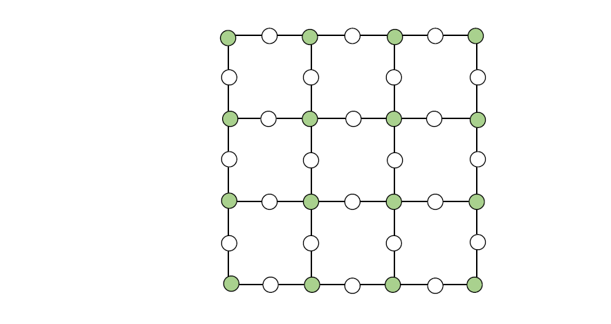
Figure 1: The 2D Lieb lattice

$\diamondsuit$

Definition 3.6

We say that a state exhibits ferromagnetism, if it has total spin $S$ such that $S=c|\Lambda|+o(|\Lambda|)$ with $c>0$. $\diamondsuit$

Theorem 3.7

Let $H_{*,n,\Lambda}\in\mathscr{C}_{\mathfrak{X}=\mathbb{C},\Lambda}^{\#}$ be given for all $L\in\mathbb{N}$. Suppose that $H_{n,\Lambda}\in\mathscr{U}(H_{*,n,\Lambda})$ for all $L$. If the ground state of $H_{*,n,\Lambda}$ exhibits ferromagnetism, then the ground state of $H_{n,\Lambda}$ exhibits ferromagnetism as well.

Proof. Let $S$ and $S_{*}$ be total spins of ground states of $H_{n,\Lambda}$ and $H_{*,n,\Lambda}$, respectively. By Theorem 3.5, we have $S=S_{*}$ for all $L\in\mathbb{N}$. Since $S_{*}=c|\Lambda|+o(|\Lambda|)$ with $c>0$, we conclude that $S=c|\Lambda|+o(|\Lambda|)$. $\Box$

3.4 Existence of long-range orders

We suppose that $H_{n,\Lambda}\in\mathscr{C}_{\Lambda}^{\#}$ acts on $\mathfrak{E}_{n,\Lambda}\otimes\mathfrak{X}_{\Lambda}$ for each $L\in\mathbb{N}$. We say that $H_{n,\Lambda}$ is translation invariant, if it holds that

$$\tau_{a}H_{n,\Lambda}\tau_{a}^{-1}=H_{n,\Lambda},\ \ \ a\in\Lambda_{\mathrm{B}}.$$ (3.8)

Here, $\tau_{a}\,(a\in\Lambda)$ on $\mathfrak{E}_{n,\Lambda}\otimes\mathfrak{X}_{\Lambda}$ is the translation such that

$$\tau_{a}c_{x\sigma}\tau_{a}^{-1}=c_{x+a\,\sigma},\ \ \ \tau_{a}\Omega=\Omega.$$ (3.9)

Example 10

We say that a matrix $\{M_{xy}\}_{x,y\in\Lambda}$ is translation invariant, if $M_{xy}=M_{x-y,o}$ for each $x,y\in\Lambda$. If $\{g_{xy}\},\ \{J_{xy}\},\ \{t_{xy}\}$ and $\{U_{xy}\}$ are translation invariant, then $H_{\mathrm{Heis}},H_{\mathrm{H}},H_{\mathrm{HH}}$ and $H_{\mathrm{rad}}$ are translation invariant. $\diamondsuit$

Example 11

Let us consider the Marshall-Lieb-Mattis Hamiltonian $H_{\mathrm{MLM}}$. Assume that $A+x=A$ and $B+x=B$ for all $x\in\Lambda_{\mathrm{B}}$. Because $\tau_{a}{\bm{S}}_{A}\tau_{a}^{-1}={\bm{S}}_{A+a}$ and $\tau_{a}{\bm{S}}_{B}\tau_{a}^{-1}={\bm{S}}_{B+a}$, $H_{\mathrm{MLM}}$ is translation invariant. $\diamondsuit$

In what follows, we assume that $H_{n,\Lambda}$ is translation invariant.

Let $\psi$ be the unique ground state of $H_{n,\Lambda}$ in the $M=0$-subspace. For each $x\in\Lambda_{\mathrm{B}}$, we define

$$\mathbb{S}_{x}^{(\pm)}=S_{x}^{(\pm)}+\sum_{j=1}^{n-1}S_{x+{\bm{e}}_{j}}^{(\pm)},$$ (3.10)

where $S_{x}^{(\pm)}=S_{x}^{(1)}+iS_{x}^{(2)}$. Here, we understand that $\mathbb{S}_{x}^{(\pm)}=S_{x}^{(\pm)}$ if $n=1$. We introduce the two-point correlation function by

$$G_{\Lambda}(x)=\Big{\langle}\psi\Big{|}\mathbb{S}_{x}^{(+)}\mathbb{S}_{o}^{(-)}\psi\Big{\rangle}=\Big{\langle}\mathbb{S}_{x}^{(+)}\mathbb{S}_{o}^{(-)}\Big{\rangle}.$$ (3.11)

By the translation invariance, we have

$$G_{\Lambda}(x-y)=\Big{\langle}\mathbb{S}_{x}^{(+)}\mathbb{S}_{y}^{(-)}\Big{\rangle},$$ (3.12)

provided that $x,y\in\Lambda_{\mathrm{B}}$. Let $\Lambda^{*}$ be the dual lattice of $\Lambda$. Let $\hat{G}_{\Lambda}(p)$ be the Fourier transformation of $G_{\Lambda}(x)$:

$$\hat{G}_{\Lambda}(p)=(2\pi)^{-d/2}\sum_{x\in\Lambda_{\mathrm{B}}}e^{-ip\cdot x}G_{\Lambda}(x),\ \ p\in\Lambda^{*}.$$ (3.13)

We have, by (3.12),

$$\hat{G}_{\Lambda}(p)=\Big{\langle}\tilde{\mathbb{S}}_{-p}^{(+)}\tilde{\mathbb{S}}_{p}^{(-)}\Big{\rangle},$$ (3.14)

where $\displaystyle\tilde{\mathbb{S}}_{p}^{(\pm)}=|\Lambda|^{-1/2}\sum_{x\in\Lambda_{\mathrm{B}}}e^{-ip\cdot x}\mathbb{S}_{x}^{(\pm)}.$ Since $(\tilde{\mathbb{S}}_{p}^{(+)})^{*}=\tilde{\mathbb{S}}_{-p}^{(-)}$, we have $\hat{G}_{\Lambda}(p)\geq 0$ for all $p\in\Lambda^{*}$.

Definition 3.8

We say that $H_{n,\Lambda}$ has long-range order with ordering wave vector $p$ (simply, LRO[$p$]) in the ground state, if it holds that

$$\liminf_{L\to\infty}\frac{\hat{G}_{\Lambda}(p)}{|\Lambda|}>0.$$ (3.15)

As for a physical interpretation of LRO, see, e.g., [54]. $\diamondsuit$

Proposition 3.9

If the ground state of $H_{n,\Lambda}$ exhibits ferromagnetism, then $H_{n,\Lambda}$ has LRO[$p=0$] in the ground state.

Proof. Since $\displaystyle\hat{G}_{\Lambda}(0)=|\Lambda|^{-1}\Big{\langle}S^{(+)}_{\mathrm{tot},n}S^{(-)}_{\mathrm{tot},n}\Big{\rangle}=\frac{|\Lambda|^{-1}}{2}\Big{\langle}S_{\mathrm{tot},n}^{2}[M=0]\Big{\rangle},$ we obtain the desired result. $\Box$

By Theorem 3.7 and Proposition 3.9, we obtain the following.

Theorem 3.10

Assume that $H_{n,\Lambda}\in\mathscr{U}(H_{*,n,\Lambda})$ for all $L$. If the ground state of $H_{*,n,\Lambda}$ exhibits ferromagnetism, then $H_{n,\Lambda}$ has LRO[$0$] in the ground state.

3.5 Proof of Theorem 1.1

Here, we prove Theorem 1.1 in Section 1.2.

(i) This immediately follows from Theorem 3.5.

(ii) We consider an extended Hilbert space $Q\mathfrak{E}_{n}\otimes\mathbb{C}^{2}$. We define a Hamiltonian $H_{1}$ acting on $Q\mathfrak{E}_{n}\otimes\mathbb{C}^{2}$ by $H_{1}=H_{*}\otimes 1-1\otimes\sigma_{1},$ where $\sigma_{1}$ is the standard Pauli matrix given by $\sigma_{1}=\begin{pmatrix}0&1\\ 1&0\end{pmatrix}$. Remark the following fact: $\mathbb{R}^{2}_{+}=\Big{\{}\begin{pmatrix}x\\ y\end{pmatrix}\in\mathbb{C}^{2}\,\Big{|}\,x,y\geq 0\Big{\}}$ is a self-dual cone in $\mathbb{C}^{2}$. Now we define a self-dual cone in $Q\mathfrak{E}_{n}[M_{*}]\otimes\mathbb{C}^{2}$ by $\mathfrak{P}_{1}=\Big{\{}\Psi_{1}\otimes\begin{pmatrix}1\\ 0\end{pmatrix}+\Psi_{2}\otimes\begin{pmatrix}0\\ 1\end{pmatrix}\Big{|}\,\Psi_{1},\Psi_{2}\in\mathfrak{P}_{*}\Big{\}}.$

Lemma 3.11

For all $s>-E(H_{1}[M_{*}])$, we have $\big{(}H_{1}[M_{*}]+s\big{)}^{-1}\rhd 0$ w.r.t. $\mathfrak{P}_{1}$.

Proof. Let $\eta=\frac{1}{\sqrt{2}}\begin{pmatrix}1\\ 1\end{pmatrix}$. We readily confirm that $\eta$ is the unique ground state of $-\sigma_{1}$ and $\eta>0$ w.r.t. $\mathbb{R}_{+}^{2}$. Let $\psi_{*}$ be the ground state of $H_{*}[M_{*}]$. By (U. 2), it holds that $\psi_{*}>0$ w.r.t. $\mathfrak{P}_{*}$. Trivially, $\psi_{*}\otimes\eta$ is the unique ground state of $H_{1}[M_{*}]$ and, by applying Corollary I.8, $\psi_{*}\otimes\eta>0$ w.r.t. $\mathfrak{P}_{1}$. Hence, by using Theorem H.10, we obtain the desired result. $\Box$

We introduce an orthogonal projection $P$ by $P\Psi\otimes r=\Psi\otimes(0,r_{2})^{T}$ for each $\Psi\in Q\mathfrak{E}_{n}[M_{*}]$ and $r=(r_{1},r_{2})^{T}\in\mathbb{C}^{2}$, where $a^{T}$ indicates the transpose of $a$. We can identify $\mathrm{ran}(P)$ with $Q\mathfrak{E}_{n}[M_{*}]$ by the isometry $\tau:\mathrm{ran}(P)\ni\Psi\otimes(0,r_{2})^{T}\mapsto r_{2}\Psi\in\mathfrak{E}_{n}[M_{*}]$. By definition, we have $P\unrhd 0$ w.r.t. $\mathfrak{P}_{1}$ and $P\mathfrak{P}_{1}=\mathfrak{P}_{*}$ by the aforementioned identification. Hence, we can readily confirm that $H_{1}[M_{*}]\leadsto H_{*}[M_{*}]$.

Next, let us consider a further extended Hilbert space $(Q\mathfrak{E}_{n}\otimes\mathbb{C}^{2})\otimes\mathbb{C}^{2}$. Define a Hamiltonian $H_{2}$ by $H_{2}=H_{1}\otimes 1-1\otimes\sigma_{1}$, and define a self-dual cone $\mathfrak{P}_{2}$ by $\mathfrak{P}_{2}=\Big{\{}\Phi_{1}\otimes\begin{pmatrix}1\\ 0\end{pmatrix}+\Phi_{2}\otimes\begin{pmatrix}0\\ 1\end{pmatrix}\Big{|}\,\Phi_{1},\Phi_{2}\in\mathfrak{P}_{1}\Big{\}}.$ Using arguments similar to those in the last paragraph. we can confirm that $H_{2}[M_{*}]\leadsto H_{1}[M_{*}]$. Repeating this procedure, we can construct a sequence of Hamiltonians $\{H_{\ell}\}$ such that $H_{\ell}[M_{*}]{\bm{\rightsquigarrow}}H_{*}[M_{*}]$. Therefore, $\mathscr{U}(H_{*})$ contains at least countably infinite number of Hamiltonians.

(iii) and (iv) immediately follow from the definition of $\mathscr{U}(H_{*,n})$. $\Box$

4 The Marshall-Lieb-Mattis stability class and stability of Lieb’s theorem

4.1 The Heisenberg model

Consider the spin-$1/2$ antiferromagnetic Heisenberg model on a finite lattice $\Lambda$. The Hamiltonian is

$$H_{\mathrm{Heis}}=\sum_{x,y\in\Lambda}J_{xy}{\bm{S}}_{x}\cdot{\bm{S}}_{y},$$ (4.1)

where $J_{xy}\geq 0$ and ${\bm{S}}_{x}=(S_{x}^{(1)},S_{x}^{(2)},S_{x}^{(3)})$.

We assume the following:

• $\Lambda$ is connected by $\{J_{xy}\}$;

• $\Lambda$ is bipartite in terms of $\{J_{xy}\}$.

$H_{\mathrm{Heis}}$ acts on the Hilbert space $\mathfrak{H}_{Q}=Q\mathfrak{E}_{n=|\Lambda|},$ where the orthogonal projection $Q$ is defined by (1.18).

Remark 4.1

The Marshall-Lieb-Mattis Hamiltonian $H_{\mathrm{MLM}}$ given by (1.17) is a special case of the Heisenberg Hamiltonian with $J_{xy}=1$ if $x\in A,\ y\in B$ or $x\in B,y\in A$, $J_{xy}=0$, otherwise. Of course, this interaction satisfies (C. 1) and (C. 2). $\diamondsuit$

4.2 The Marshall-Lieb-Mattis stability class

We will study the half-filled system, so that the Hilbert space of electron states is $\mathfrak{E}_{n=|\Lambda|}$ or $\mathfrak{H}_{Q}$. In addition, we assume that $|\Lambda|$ is even in the remainder of this section. Note that $H_{\mathrm{MLM}}\in\mathscr{C}_{\mathfrak{X}=\mathbb{C}}^{\#}$.

Definition 4.2

The $H_{\mathrm{MLM}}$- stability class $\mathscr{U}(H_{\mathrm{MLM}})$ is called the Marshall-Lieb-Mattis stability class. $\diamondsuit$

The following is a general form of stability theorems:

Theorem 4.3 (Theorem 1.4)

Suppose that $H$ is in the Marshall-Lieb-Mattis stability class. The ground state of $H$ has total spin $S=\frac{1}{2}\big{|}|A|-|B|\big{|}$ and is unique apart from the trivial $(2S+1)$-degeneracy.

We will provide a proof of Theorem 4.3 in Appendix B.

Example 12

Let us consider the following diagram:

By Theorem 4.3, the ground state of each Hamiltonian $H_{i,j}\,(i,j=1,2,\dots)$ has the total spin $S=\frac{1}{2}\big{|}|A|-|B|\big{|}$ and is unique apart from the trivial $(2S+1)$-degeneracy. $\diamondsuit$

4.3 Ferromagnetism and long-range orders in the ground state

In this subsection, we assume that $\Lambda$ has a crystal structure and every Hamiltonian is translation invariant (as for basic definitions, see Sections 3.3 and 3.4). We will specify the $\Lambda$-dependence of the Hamiltonian $H$ as $H_{\Lambda}$. Recall that the size of $\Lambda$ is determined by $L$, see Section 3.3.

By Theorems 3.7, 3.10 and 4.3, we have the following.

Theorem 4.4

Suppose that $H_{\Lambda}$ belongs to the Marshall-Lieb-Mattis stability class for each $L\in\mathbb{N}$. If there exists a constant $c>0$ independent of $\Lambda$ such that $\big{|}|A|-|B|\big{|}=c|\Lambda|$ , then the ground state of $H_{\Lambda}$ exhibits ferromagnetism. In addition, $H_{\Lambda}$ has LRO[0] in the ground state.

Example 13

Let us consider the Lieb lattice given in Example 9. We choose $A=\{{\bm{r}}+{\bm{e}}_{j}\,|\,{\bm{r}}\in\Lambda_{\mathrm{B}},j=1,2\}$ and $B=\Lambda_{\mathrm{B}}$. Then we can easily check that $\big{|}|A|-|B|\big{|}=\frac{1}{3}|\Lambda|$. Thus, if $H_{\Lambda}$ belongs to the Marshall-Lieb-Mattis stability class, then the ground state of $H$ exhibits ferromagnetism. In addition, $H_{\Lambda}$ has LRO[0] in the ground state. $\diamondsuit$

4.4 The Marshall-Lieb-Mattis theorem

We will explain the well-known Marshall-Lieb-Mattis theorem from the viewpoint of the stability class.

In this subsection, we assume (C. 1) and (C. 2).

Theorem 4.5

$H_{\mathrm{Heis}}$ is equivalent to $H_{\mathrm{MLM}}$ in the sense that $H_{\mathrm{Heis}}[M]\equiv H_{\mathrm{MLM}}[M]$ for all $M\in\mathrm{spec}\Big{(}S_{\mathrm{tot},|\Lambda|}^{(3)}\Big{)}$. (As for the definition of the binary relation “ $\equiv$”, see Definition 2.19.) In particular, $H_{\mathrm{Heis}}$ belongs to the Marshall-Lieb-Mattis stability class.

We will prove Theorem 4.5 in Appendix B.

Combining Theorems 4.3 and 4.5, we obtain the following:

Corollary 4.6 (The Marshall-Lieb-Mattis theorem[27, 24])

The ground state of $H_{\mathrm{Heis}}$ has total spin $S=\frac{1}{2}\big{|}|A|-|B|\big{|}$ and is unique apart from the trivial $(2S+1)$-degeneracy.

4.5 Lieb’s theorem

Here, we will interpret Lieb’s theorem in the context of stability class defined in Section 3.

In this subsection, we assume the following:

• (A. 1)–(A. 3).

• (C. 1), (C. 2).

Theorem 4.7

$H_{\mathrm{H},|\Lambda|}[M]\leadsto H_{\mathrm{Heis}}[M]$ for all $M\in\mathrm{spec}\Big{(}S_{\mathrm{tot},|\Lambda|}^{(3)}\Big{)}$.

We will provide a sketch of proof of Theorem 4.7 in Appendix C.

Corollary 4.8 (Theorem 1.6)

$H_{\mathrm{H},|\Lambda|}$ belongs to the Marshall-Lieb-Mattis stability class.

Proof. By Theorems 4.5 and 4.7, we have the following chain:

$$H_{\mathrm{H},|\Lambda|}[M]\leadsto H_{\mathrm{Heis}}[M]\leadsto H_{\mathrm{MLM}}[M]$$ (4.2)

for all $M\in\mathrm{spec}\Big{(}S_{\mathrm{tot},|\Lambda|}^{(3)}\Big{)}$. Thus, we conclude the assertion in the corollary. $\Box$

Corollary 4.9 (Theorem 1.6)

The ground state of $H_{\mathrm{H},|\Lambda|}$ has total spin $S=\frac{1}{2}\big{|}|A|-|B|\big{|}$ and is unique apart from the trivial $(2S+1)$-degeneracy.

Proof. This immediately follows from Theorem 4.3 and Corollary 4.8. $\Box$

4.6 Stability of Lieb’s theorem I

Let us consider the Holstein-Hubbard model at half-filling: $H_{\mathrm{HH},|\Lambda|}$. In this subsection, we assume the following:

• (A. 1)–(A. 5).

• (C. 1), (C. 2).

Let $\Omega_{\mathrm{ph}}$ be the Fock vacuum in $\mathfrak{F}_{\mathrm{ph}}$. Let us define a closed subspace of $\mathfrak{E}_{n=|\Lambda|}[M]\otimes\mathfrak{F}_{\mathrm{ph}}$ by $\mathfrak{E}_{n=|\Lambda|}[M]\otimes\Omega_{\mathrm{ph}}=\{\varphi\otimes\Omega_{\mathrm{ph}}\,|\,\varphi\in\mathfrak{E}_{n=|\Lambda|}[M]\}$. Now, we define an isometry $\tau$ from $\mathfrak{E}_{n=|\Lambda|}[M]\otimes\Omega_{\mathrm{ph}}$ onto $\mathfrak{E}_{n=|\Lambda|}[M]$ by $\tau\varphi\otimes\Omega_{\mathrm{ph}}=\varphi$. Hence, we can naturally identify $\mathfrak{E}_{n=|\Lambda|}[M]$ with $\mathfrak{E}_{n=|\Lambda|}[M]\otimes\Omega_{\mathrm{ph}}$. By this fact, $\mathfrak{E}_{n=|\Lambda|}[M]$ can be regarded as a closed subspace of $\mathfrak{E}_{n=|\Lambda|}[M]\otimes\mathfrak{F}_{\mathrm{ph}}$.

Theorem 4.10

$H_{\mathrm{HH},|\Lambda|}[M]\leadsto H_{\mathrm{H},|\Lambda|}[M]$ for all $M\in\mathrm{spec}\Big{(}S_{\mathrm{tot},|\Lambda|}^{(3)}\Big{)}$.

Remark 4.11

The Coulomb interactions in $H_{\mathrm{H}}$ and $H_{\mathrm{HH}}$ can be chosen, independently. $\diamondsuit$

We will provide a sketch of proof of Theorem 4.10 in Appendix D.

Corollary 4.12 (Theorem 1.7)

$H_{\mathrm{HH},|\Lambda|}$ belongs to the Marshall-Lieb-Mattis stability class.

Proof. By Theorems 4.5, 4.7 and 4.10, we have the following chain:

$$H_{\mathrm{HH},|\Lambda|}[M]\leadsto H_{\mathrm{H},|\Lambda|}[M]\leadsto H_{\mathrm{Heis}}[M]\leadsto H_{\mathrm{MLM}}[M]$$ (4.3)

for all $M$. Thus, $H_{\mathrm{HH},|\Lambda|}$ belongs to the Marshall-Lieb-Mattis stability class. $\Box$

Corollary 4.13 (Theorem 1.7)

The ground state of $H_{\mathrm{HH},|\Lambda|}$ has total spin $S=\frac{1}{2}\big{|}|A|-|B|\big{|}$ and is unique apart from the trivial $(2S+1)$-degeneracy.

Proof. By Theorem 4.3 and Corollary 4.12, we obtain the desired assertion. $\Box$

4.7 Stability of Lieb’s theorem II

Let us consider the many-electron system coupled to the quantized radiation field. In this subsection, we assume the following:

• (A. 1)–(A. 3).

• (C. 1), (C. 2).

Let $\Omega_{\mathrm{rad}}$ be the Fock vacuum in $\mathfrak{F}_{\mathrm{rad}}$. As before, we can regard $\mathfrak{E}_{n=|\Lambda|}[M]$ as a closed subspace of $\mathfrak{E}_{n=|\Lambda|}[M]\otimes\mathfrak{F}_{\mathrm{rad}}$ by the identification $\mathfrak{E}_{n=|\Lambda|}[M]=\mathfrak{E}_{n=|\Lambda|}[M]\otimes\Omega_{\mathrm{rad}}$.

Theorem 4.14

$H_{\mathrm{rad},|\Lambda|}[M]\leadsto H_{\mathrm{H},|\Lambda|}[M]$ for all $M\in\mathrm{spec}\Big{(}S_{\mathrm{tot},|\Lambda|}^{(3)}\Big{)}$.

We will provide a proof of Theorem 4.14 in Appendix E.

Corollary 4.15 (Theorem 1.8)

$H_{\mathrm{rad},|\Lambda|}$ belongs to the Marshall-Lieb-Mattis stability class.

Proof. By Theorems 4.5, 4.7 and 4.14, we have the following chain:

$$H_{\mathrm{rad},|\Lambda|}[M]\leadsto H_{\mathrm{H},|\Lambda|}[M]\leadsto H_{\mathrm{Heis}}[M]\leadsto H_{\mathrm{MLM}}[M]$$ (4.4)

for all $M$. Thus, $H_{\mathrm{rad},|\Lambda|}$ belongs to the Marshall-Lieb-Mattis stability class. $\Box$

By Theorem 4.3 and Corollary 4.15, we obtain the following:

Corollary 4.16 (Theorem 1.8)

The ground state of $H_{\mathrm{rad},|\Lambda|}$ has total spin $S=\frac{1}{2}\big{|}|A|-|B|\big{|}$ and is unique apart from the trivial $(2S+1)$-degeneracy.

4.8 Summary of Section 4

Our results in this section are summarized in the following diagram:

Example 14

Let us consider the Lieb lattice in Example 9. Suppose that $\{g_{xy}\},\ \{J_{xy}\},\ \{t_{xy}\}$ and $\{U_{xy}\}$ satisfy the conditions in Example 10. By the above diagram, the ground states of $H_{\mathrm{Heis}},\ H_{\mathrm{H},|\Lambda|},\ H_{\mathrm{HH},|\Lambda|}$ and $H_{\mathrm{rad},|\Lambda|}$ exhibit ferrogmanetism and LRO[0]. $\diamondsuit$

5 The Nagaoka-Thouless stability class and stability of the Nagaoka-Thouless theorem

In this section, we explain the Nagaoka-Thouless theorem from the viewpoint of stability class discussed in Section 3.

5.1 The Nagaoka-Thouless stability class

Let us consider the many-electron system with one electron less than half-filling and infinitely large Coulomb strength. The Hilbert space of electrons is $\mathfrak{H}_{\mathrm{NT}}=P_{\mathrm{G}}\mathfrak{E}_{n=|\Lambda|-1},$ where $P_{\mathrm{G}}$ is the Gutzwiller projection defined by (1.28). Recall that $P_{\mathrm{G}}$ satisfies the condition (Q). In this section, we assume

• (B. 1), (B. 2), (B. 3).

For notational simplicity, we set

$$\mathcal{S}^{2}=S_{\mathrm{tot}}^{2}\restriction\mathfrak{H}_{\mathrm{NT}},\ \ \ \mathcal{S}^{(j)}=S_{\mathrm{tot}}^{(j)}\restriction\mathfrak{H}_{\mathrm{NT}},\ \ j=1,2,3.$$ (5.1)

Note that $\mathrm{spec}(\mathcal{S}^{(3)})=\{-(|\Lambda|-1)/2,-(|\Lambda|-3)/2,\dots,(|\Lambda|-1)/2\}$. As before, the $M$-subspace of $\mathfrak{H}_{\mathrm{NT}}$ is defined by $\mathfrak{H}_{\mathrm{NT}}[M]=\ker(\mathcal{S}^{(3)}-M)$ for $M\in\mathrm{spec}(\mathcal{S}^{(3)}).$

Let $X$ be a linear operator on $\mathfrak{H}_{\mathrm{NT}}$ which commutes with $\mathcal{S}^{(3)}$. For each $M\in\mathrm{spec}(\mathcal{S}^{(3)})$, we set $X[M]=X\restriction\mathfrak{H}_{\mathrm{NT}}[M]$ as before.

Let $H_{\mathrm{H}}^{\infty}$ be the effective Hamiltonian defined in Proposition 1.10.

Definition 5.1

The $H_{\mathrm{H}}^{\infty}$-stability class $\mathscr{U}(H_{\mathrm{H}}^{\infty})$ is called the Nagaoka-Thouless stability class. $\diamondsuit$

Before we proceed, recall the Nagaoka-Thouless theorem (Theorem 1.11). The following theorem is a general form of stability of the Nagaoka-Thouless theorem:

Theorem 5.2 (Theorem 1.12)

Suppose that $H$ is in the Nagaoka-Thouless stability class. The ground state of $H$ has total spin $S=(|\Lambda|-1)/2$ and is unique apart from the trivial $(2S+1)$-degeneracy.

We will prove Theorem 5.2 in Appendix G.

Example 15

Let us consider the following diagram:

By Theorem 5.2, the ground state of each Hamiltonian $H_{i,j}\,(i,j=1,2,\dots)$ has the total spin $S=(|\Lambda|-1)/2$ and is unique apart from the trivial $(2S+1)$-degeneracy. $\diamondsuit$

5.2 Ferromagnetism and long-range orders in the ground state

In this subsection, we assume that $\Lambda$ has a crystal structure and every Hamiltonian is translation invariant. We will specify the $\Lambda$-dependence of the Hamiltonian $H$ as $H_{\Lambda}$.

By Theorems 3.7, 3.10 and 5.2, we have the following.

Theorem 5.3

Suppose that $H_{\Lambda}$ is in the Nagaoka-Thouless stability class for all $L\in\mathbb{N}$. Then the ground state of $H_{\Lambda}$ exhibits ferromagnetism. In addition, $H_{\Lambda}$ has LRO[0] in the ground state.

Example 16

Suppose that $\Lambda$ and $t_{xy}$ satisfy the conditions in Example 1. If $H_{\Lambda}$ belongs to the Nagaoka-Thouless stability class, then the ground state of $H_{\Lambda}$ exhibits ferromagnetism and LRO[0]. $\diamondsuit$

5.3 Stability of the Nagaoka-Thouless theorem I

Let $\Omega_{\mathrm{ph}}$ be the Fock vacuum in $\mathfrak{F}_{\mathrm{ph}}$. Let us define a closed subspace of $\mathfrak{H}_{\mathrm{NT}}[M]\otimes\mathfrak{F}_{\mathrm{ph}}$ by $\mathfrak{H}_{\mathrm{NT}}[M]\otimes\Omega_{\mathrm{ph}}=\{\varphi\otimes\Omega_{\mathrm{ph}}\,|\,\varphi\in\mathfrak{H}_{\mathrm{NT}}[M]\}.$ In a similar way as in Section 4.6, we can identify $\mathfrak{H}_{\mathrm{NT}}[M]$ with $\mathfrak{H}_{\mathrm{NT}}[M]\otimes\Omega_{\mathrm{ph}}$. Thus, $\mathfrak{H}_{\mathrm{NT}}[M]$ can be viewed as a closed subspace of $\mathfrak{H}_{\mathrm{NT}}[M]\otimes\mathfrak{F}_{\mathrm{ph}}$.

Let $H_{\mathrm{HH}}^{\infty}$ be the effective Hamiltonian defined in Proposition 1.14.

Theorem 5.4 (Theorem 1.15)

$H_{\mathrm{HH}}^{\infty}[M]\leadsto H_{\mathrm{H}}^{\infty}[M]$ for all $M$. In particular, $H_{\mathrm{HH}}^{\infty}$ belongs to the Nagaoka-Thouless stability class.

We will prove Theorem 5.4 in Appendix G.

By Theorems 5.2 and 5.4, we obtain the following:

Corollary 5.5 (Theorem 1.15)

The ground state of $H_{\mathrm{HH}}^{\infty}$ has total spin $S=\frac{1}{2}(|\Lambda|-1)$ and is unique apart from the trivial $(2S+1)$-degeneracy.

5.4 Stability of the Nagaoka-Thouless theorem II

In this subsection, we regard $\mathfrak{H}_{\mathrm{NT}}[M]$ as a closed subspace of $\mathfrak{H}_{\mathrm{NT}}[M]\otimes\mathfrak{F}_{\mathrm{rad}}$, as we did in Section 5.3.

Let $H_{\mathrm{rad}}^{\infty}[M]$ be the effective Hamiltonian defined in Proposition 1.16.

Theorem 5.6 (Theorem 1.17)

$H_{\mathrm{rad}}^{\infty}[M]\leadsto H_{\mathrm{H}}^{\infty}[M]$ for all $M$. In particular, $H_{\mathrm{rad}}^{\infty}$ belongs to the Nagaoka-Thouless stability class.

We will provide a proof of Theorem 5.6 in Appendix G.

By Theorems 5.2 and 5.6, we obtain the following:

Corollary 5.7 (Theorem 1.17)

The ground state of $H_{\mathrm{rad}}^{\infty}$ has total spin $S=\frac{1}{2}(|\Lambda|-1)$ and is unique apart from the trivial $(2S+1)$-degeneracy.

5.5 Summary of Section 5

Our results in this section are summarized in the following diagram:

Example 17

Assume that $\Lambda$ and $\{t_{xy}\}$ satisfy the conditions in Example 1. By Example 16 or the above diagram, the ground states of $H_{\mathrm{H}}^{\infty},\ H_{\mathrm{HH}}^{\infty}$ and $H_{\mathrm{rad}}^{\infty}$ exhibit ferromagnetism and LRO$[0]$. $\diamondsuit$

6 Concluding remarks

6.1 Why are the on-site Coulomb interactions important?

The Hubbard model with the on-site interaction has occupied an important place in the study of magnetism. In this subsection, we explain a reason for this from the viewpoint of stability class.

Let $H_{\mathrm{H}}^{(U)}$ be the Hubbard Hamiltonian $H_{\mathrm{H}}$ with the on-site Coulomb interaction:

$$U\sum_{x\in\Lambda}(n_{x}-1)^{2}$$ (6.1)

with $U>0$. In a similar way, we can define $H_{\mathrm{HH}}^{(U)}$ and $H_{\mathrm{rad}}^{(U)}$. In this subsection, we assume

• (A. 1), (A. 2).

Theorem 6.1

We have the following:

• Whenever $U>0$ and $\{U_{xy}\}$ is positive definite, we have $H_{\mathrm{H},|\Lambda|}^{(U)}[M]\equiv H_{\mathrm{H},|\Lambda|}[M]$ for all $M\in\mathrm{spec}\Big{(}S_{\mathrm{tot},|\Lambda|}^{(3)}\Big{)}$.

• Whenever $U>0$ and $\{U_{\mathrm{eff},xy}\}$ is positive definite, we have $H_{\mathrm{HH},|\Lambda|}^{(U)}[M]\equiv H_{\mathrm{HH},|\Lambda|}[M]$ for all $M\in\mathrm{spec}\Big{(}S_{\mathrm{tot},|\Lambda|}^{(3)}\Big{)}$.

• Whenever $U>0$ and $\{U_{xy}\}$ is positive definite, we have $H_{\mathrm{rad},|\Lambda|}^{(U)}[M]\equiv H_{\mathrm{rad},|\Lambda|}[M]$ for all $M\in\mathrm{spec}\Big{(}S_{\mathrm{tot},|\Lambda|}^{(3)}\Big{)}$.

We will prove Theorem 6.1 in Appendix F.

Corollary 6.2

Under the same assumptions in Theorem 6.1, we have the following:

• If the ground state of $H_{\mathrm{H},|\Lambda|}^{(U)}$ has total spin $S$, so does $H_{\mathrm{H},|\Lambda|}$.

• If the ground state of $H_{\mathrm{HH},|\Lambda|}^{(U)}$ has total spin $S$, so does $H_{\mathrm{HH},|\Lambda|}$.

• If the ground state of $H_{\mathrm{rad},|\Lambda|}^{(U)}$ has total spin $S$, so does $H_{\mathrm{rad},|\Lambda|}$.

Proof. Apply Theorems 2.11 and 6.1. $\Box$

Remark 6.3

• Theorem 6.1 and Corollary 6.2 indicate that total spin of the ground state is stable under the deformations of the Coulomb interaction.

• Lieb’s theorem tells us that $S=\frac{1}{2}\big{|}|A|-|B|\big{|}$, see Theorem 1.6.

• The Hamiltonian with the on-site Coulomb interaction is a good representative of the equivalence class, because its structure is simpler.

• Similar argument tells us that the total spin of the ground state is stable under the deformation of the hopping matrix.

• Let us consider random Coulomb interactions and random hopping matrices. Whenever the randomness is weak such that (A. 1)–(A. 3) are satisfied almost surely, we can also prove that the total spin of the ground state is stable against the randomness.

• Similar observations hold true for $H_{\mathrm{H}}^{\infty},\ H_{\mathrm{HH}}^{\infty}$ and $H_{\mathrm{rad}}^{\infty}$. $\diamondsuit$

6.2 The Su-Schrieffer-Heeger model

There are many other models which belong to the Marshall-Lieb-Mattis stability class. In this subsection, we provide an example.

The Su-Schrieffer-Heeger model is a one-dimensional model for polyacetylene [50]. The Hamiltonian is

$$H_{\mathrm{SSH}}= \sum_{j=1}^{L-1}\sum_{\sigma=\uparrow,\downarrow}\{t-\delta(Q_{j+1}-Q_{j})\}(c_{j+1\,\sigma}^{*}c_{j\sigma}+c_{j\sigma}^{*}c_{j+1\,\sigma})+U\sum_{j=1}^{L}(n_{j}-1)^{2}$$

$$+\sum_{j=1}^{L}\frac{P_{j}^{2}}{2M}+\sum_{j=1}^{L-1}\frac{K}{2}(Q_{j+1}-Q_{j})^{2},$$ (6.2)

where $Q_{j}$ and $P_{j}$ are the local phonon coordinate and momentum at site $j$. After removal of center-of-mass motion of the phonons, we obtain the following Hamiltonian [32]:

$$\hat{H}_{\mathrm{SSH}}= \sum_{j=1}^{L-1}\sum_{\sigma=\uparrow,\downarrow}f_{j}({\bm{q}})(c_{j+1\,\sigma}^{*}c_{j\sigma}+c_{j\sigma}^{*}c_{j+1\,\sigma})+U\sum_{j=1}^{L}(n_{j}-1)^{2}$$

$$+\sum_{j=1}^{L-1}\Big{(}\frac{p_{j}^{2}}{2M}+\frac{M\omega_{j}^{2}}{2}q_{j}^{2}\Big{)},$$ (6.3)

where $p_{n}=-i\partial/\partial q_{n}$ and

$$f_{j}({\bm{q}}) =t-2\delta\sqrt{\frac{2}{L}}\sum_{n=1}^{L-1}q_{n}\sin(i\theta_{n})\sin\frac{\theta_{n}}{2},\ \ \ \theta_{n}=\frac{n\pi}{L},$$ (6.4)

$$\omega_{n} =\sqrt{\frac{4K}{M}}\sin\frac{\theta_{n}}{2}.$$ (6.5)

Using the result in [32], we obtain the following:

Theorem 6.4

Let us consider the half-filled model $\hat{H}_{\mathrm{SSH},|\Lambda|}$. If $U>0$, then $\hat{H}_{\mathrm{SSH},|\Lambda|}$ belongs to the the Marshall-Lieb-Mattis stability class.

Because the nearest neighbour hopping matrix in the one-dimensional chain satisfies $|A|=|B|$, we have the following:

Corollary 6.5

The ground state of $\hat{H}_{\mathrm{SSH},|\Lambda|}$ is unique and has total spin $S=0$.

6.3 A stability class of the attractive Hubbard model

6.3.1 The attractive Hubbard model

In [25], Lieb studied the attractive Hubbard model, which forms an important stability class. We consider a model with the on-site Coulomb interaction as a representative:

$$H_{\mathrm{AH}}^{(-U)}=\sum_{x,y\in\Lambda}\sum_{\sigma=\uparrow,\downarrow}t_{xy}c_{x\sigma}^{*}c_{y\sigma}-U\sum_{x\in\Lambda}(n_{x}-1)^{2},\ \ \ U>0.$$ (6.6)

We denote by $H_{\mathrm{AH}}$ the (general) attractive Hubbard model, i.e., the Hubbard model (1.1) with the Coulomb interaction replaced by $\{-U_{xy}\}$.

From the viewpoint of stability class, Lieb’s result can be expressed as follows:

Theorem 6.6

Assume (A. 1) and (A. 3). If $U>0$, then $H_{\mathrm{AH},n}$ is equivalent to $H_{\mathrm{AH},n}^{(-U)}$ for every $n$ even. Moreover, the ground state of $H_{\mathrm{AH},n}$ is unique and has total spin $S=0$.

6.3.2 The Holstein model

The Holstein model [15] is defined by

$$H_{\mathrm{Hol}}=\sum_{x,y\in\Lambda}\sum_{\sigma=\uparrow,\downarrow}t_{xy}c_{x\sigma}^{*}c_{y\sigma}+g\sum_{x\in\Lambda}n_{x}(b_{x}+b_{x}^{*})+\omega\sum_{x\in\Lambda}b_{x}^{*}b_{x}.$$ (6.7)

Using the result in [6], we obtain the following:

Theorem 6.7

Assume (A. 1). Assume $U>0$. $H_{\mathrm{Hol},n}$ belongs to $\mathscr{U}(H_{\mathrm{AH},n}^{(-U)})$ for each $n$ even.

By Theorem 6.6, we have the following:

Corollary 6.8

Assume (A. 1). The ground state of $H_{\mathrm{Hol},n}$ is unique and has total spin $S=0$.

Remark that Corollary 6.8 is a main theorem in [6].

6.4 Other models

Here, we mention some other models. In [58, 59], Ueda, Tsunetsugu and Sigirist studied the periodic Anderson model and Kondo lattice model. They applied Lieb’s spin reflection positivity to these models and clarified the total spin in the ground states. Roughly speaking, the above-mentioned models belong to the (generalized) Marshall-Lieb-Mattis stability class. By using the methods in the present paper, the results in [58, 59] can be extended even if the electron-phonon interaction is taken into account. We will publish elsewhere the extensions.

There are several extensions of the Nagaoka-Thouless theorem; we remark that results in [19, 20, 21] can be explained in terms of the (generalized) Nagaoka-Thouless stability class.

In [45, 46, 56, 57], reader can find various models which belong to the stability classes studied in the present paper.

Finally, we conjecture that Mielke-Tasaki’s flat-band ferromagnetism [28, 29, 30, 52, 53] is related to a new stability class.

6.5 Coexistence of long-range orders

In [47], Shen, Qiu and Tian proved that ferromagnetic and antiferromagnetic long-range orders coexist in the ground state of the Hubbard model. From a viewpoint of our theory, this result can be extended as follows: In the ground state of every Hamiltonian in a certain subclass of the Marshall-Lieb-Mattis stability class, ferromagnetic and antiferromagnetic long-range orders coexist in the ground state. We will publish elsewhere this extension.

6.6 How to find a representative of stability class

Let us consider a stability class $\mathscr{U}(H_{*})$. The reader may wonder how to find the representative $H_{*}$ of stability class in actual applications. In many cases, $H_{*}$ can be obtained by a certain scaling limit: For example, the Heisenberg model is a large $U$-limit of the Hubbard model, and the Hubbard model is a large $\omega$-limit of the Holstein-Hubbard model [37]. Remark that this approach was initiated by Lieb [25]. We can also find a representative of the stability class of the Kondo and Anderson models by a suitable scaling arguments. We will publish elsewhere relations between stability classes and scaling limits.

It is noteworthy that there are some interesting similarities between the idea of scaling limit in [37] and that of the gapped quantum liquid phases [60]. To study this aspect is a future problem.

Appendix A Construction of self-dual cones

In this section, we define some self-dual cones which are important in the proofs of theorems in Section 4.

A.1 A canonical cone in $\mathscr{L}^{2}(\mathfrak{H})$

Let $\mathfrak{H}$ be a complex Hilbert space. The set of all Hilbert–Schmidt class operators on $\mathfrak{H}$ is denoted by $\mathscr{L}^{2}(\mathfrak{H})$, i.e., $\mathscr{L}^{2}(\mathfrak{H})=\{\xi\in\mathscr{B}(\mathfrak{H})\,|\,\mathrm{Tr}[\xi^{*}\xi]<\infty\}$. Henceforth, we regard $\mathscr{L}^{2}(\mathfrak{H})$ as a Hilbert space equipped with the inner product $\langle\xi|\eta\rangle_{\mathscr{L}^{2}}=\mathrm{Tr}[\xi^{*}\eta],\,\xi,\eta\in\mathscr{L}^{2}(\mathfrak{H})$.

For each $A\in\mathscr{B}(\mathfrak{H})$, the left multiplication operator is defined by

$$\mathcal{L}(A)\xi=A\xi,\ \ \xi\in\mathscr{L}^{2}(\mathfrak{H}).$$ (A.1)

Similarly, the right multiplication operator is defined by

$$\mathcal{R}(A)\xi=\xi A,\ \ \xi\in\mathscr{L}^{2}(\mathfrak{H}).$$ (A.2)

Note that $\mathcal{L}(A)$ and $\mathcal{R}(A)$ belong to $\mathscr{B}(\mathscr{L}^{2}(\mathfrak{H}))$. It is not difficult to check that

$$\mathcal{L}(A)\mathcal{L}(B)=\mathcal{L}(AB),\ \ \mathcal{R}(A)\mathcal{R}(B)=\mathcal{R}(BA),\ \ A,B\in\mathscr{B}(\mathfrak{H}).$$ (A.3)

Let $\vartheta$ be an antiunitary operator on $\mathfrak{H}$. Let $\Phi_{\vartheta}$ be an isometric isomorphism from $\mathscr{L}^{2}(\mathfrak{H})$ onto $\mathfrak{H}\otimes\mathfrak{H}$ defined by $\Phi_{\vartheta}(|x\rangle\langle y|)=x\otimes\vartheta y\ \ \ \forall x,y\in\mathfrak{H}.$ Then,

$$\mathcal{L}(A)=\Phi_{\vartheta}^{-1}A\otimes 1\Phi_{\vartheta},\ \ \ \mathcal{R}(\vartheta A^{*}\vartheta)=\Phi_{\vartheta}^{-1}1\otimes A\Phi_{\vartheta}$$ (A.4)

for each $A\in\mathscr{B}(\mathfrak{H})$. We write these facts simply as

$$\mathfrak{H}\otimes\mathfrak{H}=\mathscr{L}^{2}(\mathfrak{H}),\ \ A\otimes 1=\mathcal{L}(A),\ \ 1\otimes A=\mathcal{R}(\vartheta A^{*}\vartheta),$$ (A.5)

if no confusion arises. If $A$ is self-adjoint, then $\mathcal{L}(A)$ and $\mathcal{R}(A)$ are self-adjoint.

Recall that a bounded linear operator $\xi$ on $\mathfrak{H}$ is said to be positive if $\langle x|\xi x\rangle_{\mathfrak{H}}\geq 0$ for all $x\in\mathfrak{H}$. We write this as $\xi\geq 0$.

Definition A.1

A canonical cone in $\mathscr{L}^{2}(\mathfrak{H})$ is given by

$$\mathscr{L}^{2}(\mathfrak{H})_{+}=\Big{\{}\xi\in\mathscr{L}^{2}(\mathfrak{H})\,\Big{|}\,\mbox{$\xi$ is self-adjoint and $\xi\geq 0$ as an operator on $\mathfrak{H}$}\Big{\}}.\ \ \ \diamondsuit$$ (A.6)

Theorem A.2

$\mathscr{L}^{2}(\mathfrak{H})_{+}$ is a self-dual cone in $\mathscr{L}^{2}(\mathfrak{H})$.

Proof. Apply [35, Proposition 2.5] and Theorem H.1. $\Box$

Proposition A.3

Let $A\in\mathscr{B}(\mathfrak{H})$. We have $\mathcal{L}(A^{*})\mathcal{R}(A)\unrhd 0$ w.r.t. $\mathscr{L}^{2}(\mathfrak{H})_{+}$.

Proof. For each $\xi\in\mathscr{L}^{2}(\mathfrak{H})_{+}$, we have $\mathcal{L}(A^{*})\mathcal{R}(A)\xi=A^{*}\xi A\geq 0.$ $\Box$

Remark A.4

• In [10], Gross studied a theory of noncommutative integration in the fermionic Fock space; his framework is related to this subsection.

• Proposition A.3 is closely connected with reflection positivity, see, e.g., [8, 7]. $\diamondsuit$

A.2 The hole-particle transformations

Before we proceed, we introduce an important unitary operator $W$ as follows: The hole-particle transformation is a unitary operator $W$ on $\mathfrak{E}$ satisfying the following (i) and (ii):

• For all $x\in\Lambda$, $Wc_{x\uparrow}W^{*}=c_{x\uparrow}$ and $Wc_{x\downarrow}W^{*}=\gamma(x)c_{x\downarrow}^{*},$ where $\gamma(x)=1$ if $x\in A$, $\gamma(x)=-1$ if $x\in B$.

• $\displaystyle W\Omega=\prod_{x\in\Lambda}^{\#}c_{x\downarrow}^{*}\Omega,$ where $\Omega$ is the fermionic Fock vacuum in $\mathfrak{E}$, and $\prod_{x\in\Lambda}^{\#}$ indicates the product taken over all sites in $\Lambda$ with an arbitrarily fixed order.

The hole-particle transformations on $\mathfrak{E}\otimes\mathfrak{F}_{\mathrm{ph}}$ and $\mathfrak{E}\otimes\mathfrak{F}_{\mathrm{rad}}$ are defined by $W\otimes 1$.

Notation A.5

Let $X$ be a linear operator on $\mathfrak{Z}$. Suppose that $X$ commutes with $N_{\mathrm{el}}$ and $S_{\mathrm{tot}}^{(3)}$. We will use the following notations:

• $\tilde{X}=WXW^{-1}$;

• $\tilde{X}_{n}=WX_{n}W^{-1}$;

• $\tilde{X}_{n}[M]=WX_{n}[M]W^{-1}=\tilde{X}\restriction W\mathfrak{Z}_{n}[M]$. $\diamondsuit$

A.3 Some useful expressions of $W\mathfrak{E}_{n=|\Lambda|}[M]$ and $W\mathfrak{H}_{Q}$

Let $\mathfrak{E}(\mathfrak{X})$ be the fermionic Fock space over $\mathfrak{X}$. Remark the factorization property: $\mathfrak{E}(\mathfrak{X}_{1}\oplus\mathfrak{X}_{2})=\mathfrak{E}(\mathfrak{X}_{1})\otimes\mathfrak{E}(\mathfrak{X}_{2})$. By this fact, we have

$$\mathfrak{E}=\mathfrak{E}(\ell^{2}(\Lambda)\oplus\ell^{2}(\Lambda))=\mathfrak{E}(\ell^{2}(\Lambda))\otimes\mathfrak{E}(\ell^{2}(\Lambda)).$$ (A.7)

In this expression, the $N$-electron subspace becomes

$$\mathfrak{E}_{N}=\bigoplus_{N_{1}+N_{2}=N}\mathcal{E}^{N_{1}}\otimes\mathcal{E}^{N_{2}},$$ (A.8)

where $\mathcal{E}^{K}=\bigwedge^{K}\ell^{2}(\Lambda)$. Moreover, the $M$-subspace can be written as

$$\mathfrak{E}_{N}[M]=\mathcal{E}^{\frac{N}{2}+M}\otimes\mathcal{E}^{\frac{N}{2}-M}.$$ (A.9)

Because $\tilde{N}_{\mathrm{el}}=WN_{\mathrm{el}}W^{*}=2S^{(3)}_{\mathrm{tot}}+|\Lambda|$ and $\tilde{S}_{\mathrm{tot}}^{(3)}=WS_{\mathrm{tot}}^{(3)}W^{*}=\frac{N_{\mathrm{el}}}{2}-\frac{|\Lambda|}{2},$ we obtain, by (A.9), that

$$W\mathfrak{E}_{n=|\Lambda|}[M]=\mathfrak{E}_{n=2M+|\Lambda|}[M=0]=\mathcal{E}^{M^{\dagger}}\otimes\mathcal{E}^{M^{\dagger}},$$ (A.10)

where $M^{\dagger}=M+|\Lambda|/2$. This expression will play an important role in the present paper. Using this, we have

$$W\mathfrak{H}_{Q}[M]=\tilde{Q}\mathcal{E}^{M^{\dagger}}\otimes\mathcal{E}^{M^{\dagger}}.$$ (A.11)

The following formula will be useful:

$$\tilde{Q}=WQW^{*}=\prod_{x\in\Lambda}(n_{x}-1)^{2}.$$ (A.12)

We derive a convenient expression of $W\mathfrak{H}_{Q}[M]$ for later use. To this end, we set $\mathcal{S}=\{0,1\}^{\Lambda}$. For each ${\bm{m}}=({\bm{m}}_{\uparrow},{\bm{m}}_{\downarrow})\in\mathcal{S}\times\mathcal{S}$ with ${\bm{m}}_{\sigma}=\{m_{x\sigma}\}_{x\in\Lambda}\,(\sigma=\uparrow,\downarrow)$, we define

$$|{\bm{m}}\rangle=\prod^{\#}_{x\in\Lambda}\Big{(}c_{x\uparrow}^{*}\Big{)}^{m_{x\uparrow}}\Big{(}c_{x\downarrow}^{*}\Big{)}^{m_{x\downarrow}}\Omega.$$ (A.13)

Clearly, $\{|{\bm{m}}\rangle\,|\,{\bm{m}}\in\mathcal{S}\times\mathcal{S}\}$ is a complete orthonormal system (CONS) of $\mathfrak{E}$. Using $|{\bm{m}}\rangle$, we can represent $W\mathfrak{H}_{Q}[M]$ as

$$W\mathfrak{H}_{Q}[M]=\mathrm{Lin}\Big{\{}|{\bm{m}}\rangle\ \Big{|}\ {\bm{m}}_{\uparrow}={\bm{m}}_{\downarrow},\ \ |{\bm{m}}_{\uparrow}|=|{\bm{m}}_{\downarrow}|=M^{\dagger}\Big{\}},$$ (A.14)

where $|{\bm{m}_{\sigma}}|=\sum_{x\in\Lambda}m_{x\sigma}$.

A.4 A self-dual cone in $W\mathfrak{E}_{n=|\Lambda|}[M]$

Corresponding to the identification (A.7), we have

$$c_{x\uparrow}=\mathsf{c}_{x}\otimes 1,\ \ \ c_{x\uparrow}=(-1)^{\mathsf{N}}\otimes\mathsf{c}_{x},$$ (A.15)

where $\mathsf{c}_{x}$ is the annihilation operator on $\mathfrak{E}(\ell^{2}(\Lambda))$, and $\mathsf{N}=\sum_{x\in\Lambda}\mathsf{n}_{x}$ with $\mathsf{n}_{x}=\mathsf{c}_{x}^{*}\mathsf{c}_{x}$.

Let us define a natural self-dual cone in $W\mathfrak{E}_{n=|\Lambda|}[M]$. By the identifications (A.5) and (A.10), we have

$$W\mathfrak{E}_{n=|\Lambda|}[M]=\mathscr{L}^{2}(\mathcal{E}^{M^{\dagger}}).$$ (A.16)

Here, the antiunitary $\vartheta$ for this expression is defined as

$$\vartheta\mathsf{c}_{x}\vartheta=\mathsf{c}_{x},\ \ \ \ \vartheta\Omega=\Omega,$$ (A.17)

where $\Omega$ is the Fock vacuum in $\mathfrak{E}(\ell^{2}(\Lambda))$. (As for $\vartheta$, see Section A.1.) Now, we define a natural self-dual cone $\mathfrak{P}_{\mathrm{H}}[M]$ in $\mathscr{L}^{2}(\mathcal{E}^{M^{\dagger}})$ by

$$\mathfrak{P}_{\mathrm{H}}[M]=\mathscr{L}^{2}(\mathcal{E}^{M^{\dagger}})_{+}.$$ (A.18)

A.5 A self-dual cone in $W\mathfrak{E}_{n=|\Lambda|}[M]\otimes\mathfrak{F}_{\mathrm{ph}}$

We set $p_{x}=i\sqrt{\frac{\omega}{2}}(b_{x}^{*}-b_{x})$ and $q_{x}=\frac{1}{\sqrt{2\omega}}(b_{x}^{*}+b_{x}).$ Both operators are essentially self-adjoint. We denote their closures by the same symbols. Remark the following identification: $\mathfrak{F}_{\mathrm{ph}}=L^{2}(\mathcal{Q},d{\bm{q}})=L^{2}(\mathcal{Q}),$ where $\mathcal{Q}=\mathbb{R}^{|\Lambda|},\ d{\bm{q}}=\prod_{x\in\Lambda}dq_{x}$ is the $|\Lambda|$-dimensional Lebesgue measure on $\mathcal{Q}$, and $L^{2}(\mathcal{Q})$ is the Hilbert space of the square integrable functions on $\mathcal{Q}$. Under this identification, $q_{x}$ and $p_{x}$ can be viewed as multiplication and partial differential operators, respectively. This expression of $p_{x}$ and $q_{x}$ in $L^{2}(\mathcal{Q})$ is called the Schrödinger representation. The Hilbert space $W\mathfrak{E}_{n=|\Lambda|}[M]\otimes\mathfrak{F}_{\mathrm{ph}}$ can be identified with $W\mathfrak{E}_{n=|\Lambda|}[M]\otimes L^{2}(\mathcal{Q})$ in this representation.

A natural self-dual cone in $W\mathfrak{E}_{n=|\Lambda|}[M]\otimes\mathfrak{F}_{\mathrm{ph}}$ is defined by

$$\mathfrak{P}_{\mathrm{HH}}[M]=\int_{\mathcal{Q}}^{\oplus}\mathfrak{P}_{\mathrm{H}}[M]d{\bm{q}},$$ (A.19)

where the RHS of (A.19) is the direct integral of $\mathfrak{P}_{\mathrm{H}}[M]$, see Appendix I for details.

A.5.1 A self-dual cone in $W\mathfrak{H}_{Q}[M]$

Using the expression (A.14), we define a self-dual cone in $W\mathfrak{H}_{Q}[M]$ by

$$\mathfrak{P}_{\mathrm{Heis}}[M]=\mathrm{Coni}\Big{\{}|{\bm{m}}\rangle\ \Big{|}\ {\bm{m}}_{\uparrow}={\bm{m}}_{\downarrow},\ |{\bm{m}}_{\uparrow}|=|{\bm{m}}_{\downarrow}|=M^{\dagger}\Big{\}}.$$ (A.20)

The following property will be useful:

Proposition A.6

Under the identification (A.16), we have $\mathfrak{P}_{\mathrm{Heis}}[M]=\tilde{Q}\mathfrak{P}_{\mathrm{H}}[M],$ where $\tilde{Q}$ is given by (A.12).

Proof. Let $\varphi\in W\mathfrak{E}_{n=|\Lambda|}[M]$. $\varphi$ can be expressed as $\varphi=\sum_{{\bm{m}}_{\uparrow},{\bm{m}}_{\downarrow}\in\mathcal{S}(M^{\dagger})}\varphi_{{\bm{m}}_{\uparrow},{\bm{m}}_{\downarrow}}|{\bm{m}}\rangle,$ where $\mathcal{S}(M^{\dagger})=\{{\bm{m}\in\mathcal{S}\,|\,|{\bm{m}}|=M^{\dagger}}\}$. We say that $\{\varphi_{{\bm{m}}_{\uparrow},{\bm{m}}_{\downarrow}}\}$ is positive semidefinite, if $\sum_{{\bm{m}}_{\uparrow},{\bm{m}}_{\downarrow}\in\mathcal{S}(M^{\dagger})}\varphi_{{\bm{m}}_{\uparrow},{\bm{m}}_{\downarrow}}z^{*}_{{\bm{m}}_{\uparrow}}z_{{\bm{m}}_{\downarrow}}\geq 0$ for all ${\bm{z}}=\{z_{{\bm{m}}}\}_{{\bm{m}}\in\mathcal{S}(M^{\dagger})}\in\mathbb{C}^{|\mathcal{S}(M^{\dagger})|}$. Remark that $\varphi_{{\bm{m}}_{\uparrow},{\bm{m}}_{\downarrow}}\geq 0$ if ${\bm{m}}_{\uparrow}={\bm{m}}_{\downarrow}$ in this case.

We note that $\varphi\in\mathfrak{P}_{\mathrm{H}}[M]$ if and only if $\{\varphi_{{\bm{m}}_{\uparrow},{\bm{m}}_{\downarrow}}\}$ is positive semidefinite. To see this, we just remark that, by the definition of $\Phi_{\vartheta}$ in Section A.1, $\varphi$ can be written as $\varphi=\sum_{{\bm{m}}_{\uparrow},{\bm{m}}_{\downarrow}\in\mathcal{S}(M^{\dagger})}\varphi_{{\bm{m}}_{\uparrow},{\bm{m}}_{\downarrow}}|{\bm{m}}_{\uparrow}\rangle\langle{\bm{m}}_{\downarrow}|.$ Here, we used the fact that $|\vartheta{\bm{m}}_{\downarrow}\rangle=|{\bm{m}}_{\downarrow}\rangle$ by (A.17).

For each $x\in\Lambda$, we observe that $(n_{x}-1)^{2}|{\bm{m}}\rangle\neq 0$, if and only if $m_{x\uparrow}=m_{x\downarrow}$. Hence, $\tilde{Q}|{\bm{m}}\rangle\neq 0$, if and only if ${\bm{m}}_{\uparrow}={\bm{m}}_{\downarrow}$. Therefore, for each $\varphi\in\mathfrak{P}_{\mathrm{H}}[M]$, we obtain

$$\tilde{Q}\varphi=\sum_{{\bm{m}}_{\uparrow}={\bm{m}}_{\downarrow}\in\mathcal{S}(M^{\dagger})}\varphi_{{\bm{m}}_{\uparrow},{\bm{m}}_{\downarrow}}|{\bm{m}}\rangle.$$ (A.21)

Because $\varphi_{{\bm{m}}_{\uparrow},{\bm{m}}_{\downarrow}}\geq 0$ provided that ${\bm{m}}_{\uparrow}={\bm{m}}_{\downarrow}$, the RHS of (A.21) belongs to $\mathfrak{P}_{\mathrm{Heis}}[M]$. $\Box$

Appendix B Proof of Theorems 4.3 and 4.5

In this appendix, we will prove Theorems 4.3 and 4.5. Because several notations are defined in Appendix A, the reader is suggested to study Appendix A first.

B.1 Basic properties of $H_{\mathrm{Heis}}$

For each $x,y\in\Lambda$ with $x\neq y$ and $\sigma\in\{\uparrow,\downarrow\}$, set $A_{xy\sigma}=c_{x\sigma}c_{y\sigma}^{*}.$ One can express $H_{\mathrm{Heis}}$ as

$$H_{\mathrm{Heis}} =\sum_{x,y\in\Lambda}\frac{J_{xy}}{2}\bigg{\{}-(A_{xy\uparrow}A_{xy\downarrow}^{*}+A_{xy\uparrow}^{*}A_{xy\downarrow})+\frac{1}{2}(n_{x\uparrow}-n_{x\downarrow})(n_{y\uparrow}-n_{y\downarrow})\bigg{\}}.$$ (B.1)

By the hole-particle transformation $W$, we have $\tilde{H}_{\mathrm{Heis}}=WH_{\mathrm{Heis}}W^{-1}=-T+V,$ where

$$T=\sum_{x,y\in\Lambda}\frac{J_{xy}}{2}(A_{xy\uparrow}^{*}A_{xy\downarrow}^{*}+A_{xy\uparrow}A_{xy\downarrow}),\ \ \ V=\sum_{x,y\in\Lambda}\frac{J_{xy}}{4}(n_{x}-1)(n_{y}-1).$$ (B.2)

For each $x,y\in\Lambda$, we set $T_{xy}=\frac{J_{xy}}{2}A_{xy\uparrow}A_{xy\downarrow}.$ Trivially, we have $T=\sum_{x,y\in\Lambda}(T_{xy}+T_{xy}^{*})$.

Lemma B.1

Let $x,y\in\Lambda$ with $x\neq y$. For all ${\bm{m}}=({\bm{m}}_{\uparrow},{\bm{m}}_{\downarrow})\in\mathcal{S}\times\mathcal{S}$ with ${\bm{m}}_{\uparrow}={\bm{m}}_{\downarrow}$, we have the following:

• $\displaystyle T_{xy}|{\bm{m}}\rangle=\frac{J_{xy}}{2}\big{|}{\bm{m}_{\uparrow}-{\bm{\delta}}_{x}+{\bm{\delta}}_{y}},{\bm{m}_{\downarrow}-{\bm{\delta}}_{x}+{\bm{\delta}}_{y}}\big{\rangle}$, where ${\bm{\delta}}_{a}=\{\delta_{ax}\}_{x\in\Lambda}$.

• $\displaystyle T_{xy}^{*}|{\bm{m}}\rangle=\frac{J_{xy}}{2}\big{|}{\bm{m}_{\uparrow}+{\bm{\delta}}_{x}-{\bm{\delta}}_{y}},{\bm{m}_{\downarrow}+{\bm{\delta}}_{x}-{\bm{\delta}}_{y}}\big{\rangle}$.

In the above, we understand that

$$\big{|}{\bm{m}_{\uparrow}-{\bm{\delta}}_{x}+{\bm{\delta}}_{y}},{\bm{m}_{\downarrow}-{\bm{\delta}}_{x}+{\bm{\delta}}_{y}}\big{\rangle}=0$$ (B.3)

if $m_{\uparrow x}=0$ or $m_{\uparrow y}=1$ or $m_{\downarrow x}=0$ or $m_{\downarrow y}=1$, and

$$\big{|}{\bm{m}_{\uparrow}+{\bm{\delta}}_{x}-{\bm{\delta}}_{y}},{\bm{m}_{\downarrow}+{\bm{\delta}}_{x}-{\bm{\delta}}_{y}}\big{\rangle}=0$$ (B.4)

if $m_{\uparrow x}=1$ or $m_{\uparrow y}=0$ or $m_{\downarrow x}=1$ or $m_{\downarrow y}=0$.

Proof. This lemma immediately follows from (A.13) and (B.1). $\Box$

Let $\mathfrak{P}_{\mathrm{Heis}}[M]$ be the self-dual cone in $W\mathfrak{H}_{Q}[M]$ defined by (A.20).

Lemma B.2

We have $T_{xy}\unrhd 0$ w.r.t. $\mathfrak{P}_{\mathrm{Heis}}[M]$. Therefore, we have $T\unrhd 0$ and $e^{\beta T}\unrhd 0$ w.r.t. $\mathfrak{P}_{\mathrm{Heis}}[M]$ for all $\beta\geq 0$.

Proof. By Lemma B.1, we immediately get $T_{xy}\unrhd 0$ w.r.t. $\mathfrak{P}_{\mathrm{Heis}}[M]$, which implies that $T\unrhd 0$ w.r.t. $\mathfrak{P}_{\mathrm{Heis}}[M]$. Thus, applying Proposition H.7, we conclude that $e^{\beta T}\unrhd 0$ w.r.t. $\mathfrak{P}_{\mathrm{Heis}}[M]$ for all $\beta\geq 0$. $\Box$

Lemma B.3

$e^{-\beta V}\unrhd 0$ w.r.t. $\mathfrak{P}_{\mathrm{Heis}}[M]$ for all $\beta\geq 0$.

Proof. Since $n_{x}|{\bm{m}}\rangle=(m_{x\uparrow}+m_{x\downarrow})|{\bm{m}}\rangle$, every $|{\bm{m}}\rangle$ is an eigenvector of $V$: $V|{\bm{m}}\rangle=V({\bm{m}})|{\bm{m}}\rangle$, where $V({\bm{m}})$ is the corresponding eigenvalue. Hence, $e^{-\beta V}|{\bm{m}}\rangle=e^{-\beta V({\bm{m}})}|{\bm{m}}\rangle$, which implies $e^{-\beta V}\unrhd 0$ w.r.t. $\mathfrak{P}_{\mathrm{Heis}}[M]$. $\Box$

Proposition B.4

$e^{-\beta\tilde{H}_{\mathrm{Heis}}[M]}\unrhd 0$ w.r.t. $\mathfrak{P}_{\mathrm{Heis}}[M]$ for all $\beta\geq 0$.

Proof. By Lemmas B.2, B.3 and Theorem H.9, we arrive at the assertion in the proposition. $\Box$

Theorem B.5

Assume (C. 1) and (C. 2). We have $\big{(}\tilde{H}_{\mathrm{Heis}}[M]+s\big{)}^{-1}\rhd 0$ w.r.t. $\mathfrak{P}_{\mathrm{Heis}}[M]$ for all $s>-E\big{(}\tilde{H}_{\mathrm{Heis}}[M]\big{)}$. In particular, $\big{(}\tilde{H}_{\mathrm{MLM}}[M]+s\big{)}^{-1}\rhd 0$ w.r.t. $\mathfrak{P}_{\mathrm{Heis}}[M]$ for all $s>-E\big{(}\tilde{H}_{\mathrm{MLM}}[M]\big{)}$.

Proof. Before we will enter the proof, we remark the following. Let $\psi\in\mathfrak{P}_{\mathrm{Heis}}[M]$. Set $S_{M}=\{{\bm{m}}=({\bm{m}}_{\uparrow},{\bm{m}}_{\downarrow})\in\mathcal{S}\times\mathcal{S}\,|\,{\bm{m}}_{\uparrow}={\bm{m}}_{\downarrow},\ |{\bm{m}}_{\uparrow}|=|{\bm{m}}_{\downarrow}|=M^{\dagger}\}$. We can express $\psi$ as $\psi=\sum_{{\bm{m}}\in S_{M}}\psi({\bm{m}})|{\bm{m}}\rangle$ with $\psi({\bm{m}})\geq 0$ for all ${\bm{m}}\in S_{M}$.

We will apply Theorem H.15 with $A=-T$ and $B=V$. To this end, we will check all assumptions in the theorem.

The assumption (b) is satisfied by Lemma B.3. To check (a) and (c), we set $V_{n}=(1-e^{-n})V,\ n\in\mathbb{N}$. Trivially, $-T+V_{n}$ converges to $\tilde{H}_{\mathrm{Heis}}[M]$, and $\tilde{H}_{\mathrm{Heis}}[M]-V_{n}$ converges to $-T$ in the uniform topology as $n\to\infty$. Thus, the assumption (a) is fulfilled. To see (c), take $\psi,\psi^{\prime}\in\mathfrak{P}_{\mathrm{Heis}}[M]$. Suppose that $\langle\psi|\psi^{\prime}\rangle=0$. We can express these as

$$\psi=\sum_{{\bm{m}}\in S_{M}}\psi({\bm{m}})|{\bm{m}}\rangle,\ \ \ \psi^{\prime}{}=\sum_{{\bm{m}}\in S_{M}}\psi^{\prime}{}({\bm{m}})|{\bm{m}}\rangle$$ (B.5)

with $\sum_{{\bm{m}}\in S_{M}}\psi({\bm{m}})\psi^{\prime}({\bm{m}})=0$. Because $\psi({\bm{m}})$ and $\psi^{\prime}({\bm{m}})$ are nonnegative, we conclude $\psi(\bm{m})\psi^{\prime}(\bm{m})=0$ for all ${\bm{m}}\in S_{M}$. Thus,

$$\langle\psi|e^{-\beta V_{n}}\psi^{\prime}\rangle=\sum_{{\bm{m}}\in S_{M}}\psi(\bm{m})\psi^{\prime}(\bm{m})e^{-\beta(1-e^{-n})V({\bm{m}})}=0,$$ (B.6)

where $V({\bm{m}})$ is defined in the proof of Lemma B.3. Therefore, (c) is satisfied.

Choose $\psi,\psi^{\prime}{}\in\mathfrak{P}_{\mathrm{Heis}}[M]\backslash\{0\}$, arbitrarily. Again we express these vectors as (B.5). Since $\psi$ and $\psi^{\prime}{}$ are nonzero, there exist ${\bm{m}},{\bm{m}}^{\prime}{}\in S_{M}$ such that $\psi({\bm{m}})>0$ and $\psi^{\prime}{}({\bm{m}^{\prime}{}})>0$. Because $\psi\geq\psi({\bm{m}})|{\bm{m}}\rangle$ and $\psi^{\prime}{}\geq\psi^{\prime}{}({\bm{m}}^{\prime}{})|{\bm{m}}^{\prime}{}\rangle$ w.r.t. $\mathfrak{P}_{\mathrm{Heis}}[M]$, we see that

$$\langle\psi|e^{\beta T}|\psi^{\prime}{}\rangle\geq\psi({\bm{m}})\psi^{\prime}{}({\bm{m}}^{\prime}{})\langle{\bm{m}}|e^{\beta T}|{\bm{m}}^{\prime}{}\rangle$$ (B.7)

by Lemma B.2.

By Lemma B.2 again, we have

$$e^{\beta T}=\sum_{n=0}^{\infty}\frac{\beta^{n}}{n!}T^{n}\unrhd\frac{\beta^{\ell}}{\ell!}T^{\ell}$$ (B.8)

w.r.t. $\mathfrak{P}_{\mathrm{Heis}}[M]$ for all $\beta\geq 0$ and $\ell\in\mathbb{N}_{0}$. On the other hand, using the assumption (C. 1) and Lemma B.2, there are sequencces $\{x_{1},x_{2},\dots,x_{\ell};y_{1},y_{2},\dots,y_{\ell}\}$ and $\{\#_{1},\dots,\#_{\ell}\}\in\{{\pm}\}^{\ell}$such that

$$\Big{\langle}{\bm{m}}\Big{|}T_{x_{1}y_{1}}^{\#_{1}}T_{x_{2}y_{2}}^{\#_{2}}\cdots T_{x_{\ell}y_{\ell}}^{\#_{\ell}}\Big{|}{\bm{m}}^{\prime}{}\Big{\rangle}>0,$$ (B.9)

where $a^{\#}=a$ if $\#=-$, $a^{\#}=a^{*}$ if $\#=+$. Since $T\unrhd T_{xy}$ for all $x,y\in\Lambda$, we have

$$T^{\ell}\unrhd T_{x_{1}y_{1}}^{\#_{1}}T_{x_{2}y_{2}}^{\#_{2}}\cdots T_{x_{\ell}y_{\ell}}^{\#_{\ell}}$$ (B.10)

w.r.t. $\mathfrak{P}_{\mathrm{Heis}}[M]$ for all $\beta\geq 0$. Combining (B.8), (B.9) and (B.10), we obtain

$$\langle{\bm{m}}|e^{\beta T}|{\bm{m}}^{\prime}{}\rangle\geq\frac{\beta^{\ell}}{\ell!}\Big{\langle}{\bm{m}}\Big{|}T_{x_{1}y_{1}}^{\#_{1}}T_{x_{2}y_{2}}^{\#_{2}}\cdots T_{x_{\ell}y_{\ell}}^{\#_{\ell}}\Big{|}{\bm{m}}^{\prime}{}\Big{\rangle}>0.$$ (B.11)

By this and (B.7), we conclude that $e^{\beta T}\rhd 0$ w.r.t. $\mathfrak{P}_{\mathrm{Heis}}[M]$ for all $\beta>0$. Therefore, we conclude that, by Theorem H.15, $e^{-\beta\tilde{H}_{\mathrm{Heis}}[M]}\rhd 0$ w.r.t. $\mathfrak{P}_{\mathrm{Heis}}[M]$ for all $\beta>0$. Because $H_{\mathrm{MLM}}$ is a special case of the Heisenberg model, we also get $e^{-\beta\tilde{H}_{\mathrm{MLM}}[M]}\rhd 0$ w.r.t. $\mathfrak{P}_{\mathrm{Heis}}[M]$ for all $\beta>0$. By applying Proposition H.6, we obtain the desired result in Theorem B.5. $\Box$

B.2 Proof of Theorem 4.3

We begin with the following proposition [27, 24]:

Proposition B.6

The ground state of $H_{\mathrm{MLM}}$ has total spin $S=\frac{1}{2}\big{|}|A|-|B|\big{|}$ and is unique apart from the trivial $(2S+1)$-degeneracy.

Proof. By Theorems H.10 and B.5, the ground state of $H_{\mathrm{MLM}}[M]$ is unique for all $M\in\mathrm{spec}\Big{(}S_{\mathrm{tot},|\Lambda|}^{(3)}\Big{)}$. Let us work in the $M=0$ subspace. Since $2H_{\mathrm{MLM}}=({\bm{S}}_{A}+{\bm{S}}_{B})^{2}-{\bm{S}}_{A}^{2}-{\bm{S}}_{B}^{2}$, we see that the ground state of $H_{\mathrm{MLM}}[M=0]$ has total spin $S=\frac{1}{2}\big{|}|A|-|B|\big{|}$. We denote by $\varphi_{0}$ the ground state of $H_{\mathrm{MLM}}[0]$. Let $S_{\mathrm{tot}}^{(\pm)}=S_{\mathrm{tot}}^{(1)}\pm iS_{\mathrm{tot}}^{(2)}.$ We set $\varphi_{M}=(S_{\mathrm{tot}}^{(+)})^{M}\varphi_{0}$ for $M>0$ and $\varphi_{M}=(S_{\mathrm{tot}}^{(-)})^{|M|}\varphi_{0}$ for $M<0$. Because $H_{\mathrm{MLM}}$ commutes with $S_{\mathrm{tot}}^{(\pm)}$, we know that $\varphi_{M}$ is the unique ground state of $H_{\mathrm{MLM}}[M]$ which has total spin $S=\frac{1}{2}\big{|}|A|-|B|\big{|}$. Thus, the ground state of $H_{\mathrm{MLM}}$ is unique apart from the trivial $(2S+1)$-degeneracy. $\Box$

Completion of proof of Theorem 4.3

By applying Theorem 3.5 and Proposition B.6, one obtains Theorem 4.3. $\Box$

B.3 Proof of Theorem 4.5

By Theorem B.5, we can check all conditions in Definition 2.9 with

$$(H,\ H_{*};\ \mathfrak{H},\ \mathfrak{H}_{*};\ P;\ \mathfrak{P},\ \mathfrak{P}_{*};O;U)$$

$$= \Big{(}\tilde{H}_{\mathrm{Heis}}[M],\,\tilde{H}_{\mathrm{MLM}}[M];\,W\mathfrak{H}_{Q}[M],\ W\mathfrak{H}_{Q}[M];1;\,\mathfrak{P}_{\mathrm{Heis}}[M],\,\mathfrak{P}_{\mathrm{Heis}}[M];\tilde{S}_{\mathrm{tot},|\Lambda|}^{2}[M];1\Big{)}.$$

Hence, $\tilde{H}_{\mathrm{Heis}}[M]\leadsto\tilde{H}_{\mathrm{MLM}}[M]$ for all $M\in\mathrm{spec}\Big{(}S_{\mathrm{tot},|\Lambda|}^{(3)}\Big{)}$.

By interchanging the roles of $H_{\mathrm{Heis}}$ and $H_{\mathrm{MLM}}$ in the above, we have $\tilde{H}_{\mathrm{MLM}}[M]\leadsto\tilde{H}_{\mathrm{Heis}}[M]$ for all $M\in\mathrm{spec}\Big{(}S_{\mathrm{tot},|\Lambda|}^{(3)}\Big{)}$. Thus, $\tilde{H}_{\mathrm{MLM}}[M]\equiv\tilde{H}_{\mathrm{Heis}}[M]$. By applying Proposition 2.10 with $V=W$, we conclude that $H_{\mathrm{MLM}}[M]\equiv H_{\mathrm{Heis}}[M]$. Especially, $H_{\mathrm{Heis}}$ belongs to the Marshall-Lieb-Mattis stability class. $\Box$

Appendix C Proof of Theorem 4.7

Because several notations are defined in Appendix A, the reader is suggested to study Appendix A first.

C.1 Basic materials

C.1.1 Properties of $\tilde{Q}$

Let $\mathfrak{P}_{\mathrm{H}}[M]$ be the self-dual cone in $W\mathfrak{E}_{n=|\Lambda|}[M]$ defined by (A.18). Recall that $\tilde{Q}$ is defined by $\tilde{Q}=WQW^{-1}$, see Notation A.5 for more details.

Proposition C.1

We have $\tilde{Q}\unrhd 0$ w.r.t. $\mathfrak{P}_{\mathrm{H}}[M]$ for all $M\in\mathrm{spec}\Big{(}S_{\mathrm{tot},|\Lambda|}^{(3)}\Big{)}$.

Proof. Recall the formula (A.12). Set $q_{x}=(1-n_{x})^{2}$. Since

$$q_{x}=1-n_{x}+2n_{x\uparrow}n_{x\downarrow}=1-\mathcal{L}({\mathsf{n}}_{x})-\mathcal{R}(\mathsf{n}_{x})+2\mathcal{L}(\mathsf{n}_{x})\mathcal{R}(\mathsf{n}_{x}),$$ (C.1)

we have, by Theorem H.12,

$$e^{tq_{x}}\unrhd 0\ \ \ \mbox{ w.r.t. $\mathfrak{P}_{\mathrm{H}}[M]$ for all $t\geq 0$.}$$ (C.2)

Because $q_{x}$ is an orthogonal projection, we have

$$e^{tq_{x}}=1+q_{x}(e^{t}-1)=q_{x}^{\perp}+q_{x}e^{t}.$$ (C.3)

By (C.2) and (C.3), we obtain $e^{-t}q_{x}^{\perp}+q_{x}\unrhd 0$ w.r.t. $\mathfrak{P}_{\mathrm{H}}[M]$. Taking $t\to\infty$, we arrive at $q_{x}\unrhd 0$ w.r.t. $\mathfrak{P}_{\mathrm{H}}[M]$, which implies that $\displaystyle\tilde{Q}=\prod_{x\in\Lambda}q_{x}\unrhd 0$ w.r.t. $\mathfrak{P}_{\mathrm{H}}[M]$. $\Box$

C.1.2 Properties of $\tilde{H}_{\mathrm{H},|\Lambda|}[M]$

First, we remark that, by the hole-particle transformation, the Coulomb interaction term becomes

$$W\sum_{x,y\in\Lambda}\frac{U_{xy}}{2}(n_{x}-1)(n_{y}-1)W^{-1}=\sum_{x,y\in\Lambda}\frac{U_{xy}}{2}(n_{x\uparrow}-n_{x\downarrow})(n_{y\uparrow}-n_{y\downarrow}).$$ (C.4)

Using the identification (A.16), we can express $\tilde{H}_{\mathrm{H},|\Lambda|}[M]$ as $\tilde{H}_{\mathrm{H},|\Lambda|}[M]=\mathbb{T}-\mathbb{U},$ where

$$\mathbb{T}=\mathcal{L}(T)+\mathcal{R}(T),\ \ \ T=\sum_{x,y\in\Lambda}\bigg{(}t_{xy}\mathsf{c}_{x}^{*}\mathsf{c}_{y}+\frac{U_{xy}}{2}\mathsf{n}_{x}\mathsf{n}_{y}\bigg{)}$$ (C.5)

and $\mathbb{U}=\sum_{x,y\in\Lambda}U_{xy}\mathcal{L}(\mathsf{n}_{x})\mathcal{R}(\mathsf{n}_{y}).$ Here, recall that $\mathsf{c}_{x}$ and $\mathsf{n}_{x}$ are defined in Section A.4. Also, recall that $\mathcal{L}(\cdot)$ and $\mathcal{R}(\cdot)$ are defined in Section A.1.

Lemma C.2

We have $\mathbb{U}\unrhd 0$ w.r.t. $\mathfrak{P}_{\mathrm{H}}[M]$.

Proof. Since $\mathbf{U}=\{U_{xy}\}_{x,y}$ is a positive definite matrix by (A. 3), all eigenvalues $\{\lambda_{x}\}_{x\in\Lambda}$ of $\mathbf{U}$ are strictly positive, and there exists an orthogonal matrix $\mathbf{P}$ such that $\mathbf{U}=\mathbf{P}\mathbf{D}\mathbf{P}^{\mathrm{T}}$, where $\mathbf{D}=\mathrm{diag}(\lambda_{x})$. We set $\mathbf{n}=\{\mathsf{n}_{x}\}_{x\in\Lambda}$ and set $\hat{\mathbf{n}}=\mathbf{P}^{\mathrm{T}}\mathbf{n}$. Denoting $\hat{\mathbf{n}}=\{\hat{\mathsf{n}}_{x}\}_{x\in\Lambda}$, we have

$$\mathbb{U}=\big{\langle}\mathcal{L}(\mathbf{n})|\mathbf{U}\mathcal{R}(\mathbf{n})\big{\rangle}=\big{\langle}\mathcal{L}(\hat{\mathbf{n}})|\mathbf{D}\mathcal{R}(\hat{\mathbf{n}})\big{\rangle}=\sum_{x\in\Lambda}\lambda_{x}\mathcal{L}(\hat{\mathsf{n}}_{x})\mathcal{R}(\hat{\mathsf{n}}_{x})\unrhd 0.$$ (C.6)

This completes the proof. $\Box$

Proposition C.3

We have $\big{(}\tilde{H}_{\mathrm{H},|\Lambda|}[M]+s\big{)}^{-1}\unrhd 0$ w.r.t. $\mathfrak{P}_{\mathrm{H}}[M]$ for all $s>-E\big{(}\tilde{H}_{\mathrm{H},|\Lambda|}[M]\big{)}$.

Proof. We remark that $\mathbb{U}\unrhd 0$ w.r.t. $\mathfrak{P}_{\mathrm{H}}[M]$ by Lemma C.2, and

$$e^{-\beta\mathbb{T}}=\mathcal{L}(e^{-\beta T})\mathcal{R}(e^{-\beta T})\unrhd 0\ \ \mbox{w.r.t. $\mathfrak{P}_{\mathrm{H}}[M]$}.$$ (C.7)

Therefore, by Theorem H.8, we have $e^{-\beta\tilde{H}_{\mathrm{H},|\Lambda|}[M]}\unrhd 0$ w.r.t. $\mathfrak{P}_{\mathrm{H}}[M]$ for all $\beta>0$. By applying Proposition H.5, we conclude the assertion in Proposition C.3. $\Box$

In [32, Theorem 4.6], we proved the following stronger result:

Theorem C.4

We have $\big{(}\tilde{H}_{\mathrm{H},|\Lambda|}[M]+s\big{)}^{-1}\rhd 0$ w.r.t. $\mathfrak{P}_{\mathrm{H}}[M]$ for all $s>-E\big{(}\tilde{H}_{\mathrm{H},|\Lambda|}[M]\big{)}$.

C.2 Completion of proof of Theorem 4.7

We will check all conditions in Definition 2.9 with

$$(H,\ H_{*};\ \mathfrak{H},\ \mathfrak{H}_{*};\ P;\ \mathfrak{P},\ \mathfrak{P}_{*};O;U)$$

$$= \Big{(}\tilde{H}_{\mathrm{H},|\Lambda|}[M],\,\tilde{H}_{\mathrm{Heis}}[M];\,W\mathfrak{E}_{n=|\Lambda|}[M],\ W\mathfrak{H}_{Q}[M];\,\tilde{Q};\,\mathfrak{P}_{\mathrm{H}}[M],\,\mathfrak{P}_{\mathrm{Heis}}[M];\ \tilde{S}_{\mathrm{tot},|\Lambda|}^{2}[M];1\Big{)}.$$

By Proposition C.1, (i) of Definition 2.9 is satisfied. (ii) of Definition 2.9 follows from Proposition A.6. (iii) and (iv) of Definition 2.9 follow from Theorem C.4 and Theorem B.5, respectively. Taking Proposition 2.10 (with $V=W$) into consideration, we obtain Theorem 4.7. $\Box$

Appendix D Proof of Theorem 4.10

D.1 Basic materials

D.1.1 Properties of $P_{\mathrm{ph}}$

Let $P_{\mathrm{ph}}=1\otimes|\Omega_{\mathrm{ph}}\rangle\langle\Omega_{\mathrm{ph}}|$. Let $\mathfrak{P}_{\mathrm{HH}}[M]$ be the self-dual cone in $W\mathfrak{E}_{n=|\Lambda|}[M]\otimes\mathfrak{F}_{\mathrm{ph}}$ defined by (A.19).

Proposition D.1

We have $P_{\mathrm{ph}}\unrhd 0$ w.r.t. $\mathfrak{P}_{\mathrm{HH}}[M]$ for all $M\in\mathrm{spec}\Big{(}S_{\mathrm{tot},|\Lambda|}^{(3)}\Big{)}$.

Proof. Remark that, in the Schrödinger representation, the Fock vacuum $\Omega_{\mathrm{ph}}$ can be expressed as $\Omega_{\mathrm{ph}}({\bm{q}})=\pi^{-|\Lambda|/4}\exp(-{\bm{q}}^{2}/2)$, which is strictly positive for all ${\bm{q}}$. Hence, for each $\varphi\in L^{2}(\mathcal{Q})_{+}$, we have $\langle\Omega_{\mathrm{ph}}|\varphi\rangle\geq 0$, which implies that $|\Omega_{\mathrm{ph}}\rangle\langle\Omega_{\mathrm{ph}}|\unrhd 0$ w.r.t. $L^{2}(\mathcal{Q})_{+}$. Thus, by Corollary I.4, we conclude the assertion in Proposition D.1. $\Box$

Proposition D.2

Under the identification by $\tau$ in Section 4.6, we have $P_{\mathrm{ph}}\mathfrak{P}_{\mathrm{HH}}[M]=\mathfrak{P}_{\mathrm{H}}[M]$ for all $M\in\mathrm{spec}\Big{(}S_{\mathrm{tot},|\Lambda|}^{(3)}\Big{)}$.

Proof. It is easily checked that $P_{\mathrm{ph}}\mathfrak{P}_{\mathrm{HH}}[M]=\mathfrak{P}_{\mathrm{H}}[M]\otimes\Omega_{\mathrm{ph}}$. Hence, by the identification in Section 4.6, we obtain the desired result. $\Box$

D.1.2 Properties of $\tilde{H}_{\mathrm{HH},|\Lambda|}[M]$

We work in the Schrödinger representation introduced in Section A.5. Let

$$L=-i\sqrt{2}\omega^{-3/2}\sum_{x,y\in\Lambda}g_{xy}(n_{x\uparrow}-n_{x\downarrow})p_{y}.$$ (D.1)

$L$ is essentially anti-self-adjoint. We denote its closure by the same symbol. A unitary operator $e^{L}$ is called the Lang-Firsov transformation [23]. We remark the following properties:

$$e^{L}c_{x\uparrow}e^{-L} =\exp\Bigg{\{}+i\sqrt{2}\omega^{-3/2}\sum_{y\in\Lambda}g_{xy}p_{y}\Bigg{\}}c_{x\uparrow},$$ (D.2)

$$e^{L}c_{x\downarrow}e^{-L} =\exp\Bigg{\{}-i\sqrt{2}\omega^{-3/2}\sum_{y\in\Lambda}g_{xy}p_{y}\Bigg{\}}c_{x\downarrow},$$ (D.3)

$$e^{L}b_{x}e^{-L} =b_{x}-\omega^{-1}\sum_{y\in\Lambda}g_{xy}(n_{y\uparrow}-n_{y\downarrow}).$$ (D.4)

The following facts will be used:

$$e^{-i\frac{\pi}{2}N_{\mathrm{ph}}}q_{x}e^{i\frac{\pi}{2}N_{\mathrm{ph}}}=\omega^{-1}p_{x},\ \ \ e^{-i\frac{\pi}{2}N_{\mathrm{ph}}}p_{x}e^{i\frac{\pi}{2}N_{\mathrm{ph}}}=\omega q_{x},$$ (D.5)

where $N_{\mathrm{ph}}=\sum_{x\in\Lambda}b_{x}^{*}b_{x}=\frac{1}{2}\sum_{x\in\Lambda}(p_{x}^{2}+\omega^{2}q_{x}^{2}-1)$.

Lemma D.3

Set $\mathscr{U}=e^{-i\frac{\pi}{2}N_{\mathrm{ph}}}e^{L}$. We have

$$\mathscr{U}\tilde{H}_{\mathrm{HH},|\Lambda|}\mathscr{U}^{*}=T_{+g,\uparrow}+T_{-g,\downarrow}+\tilde{U}_{\mathrm{eff}}+E_{\mathrm{ph}}+\mathrm{Const.},$$ (D.6)

where

$$T_{\pm g,\sigma} =\sum_{x,y\in\Lambda}t_{xy}\exp\big{\{}\pm i\Phi_{xy}\big{\}}c_{x\sigma}^{*}c_{y\sigma},$$ (D.7)

$$\Phi_{xy} =\sqrt{2}\omega^{-1/2}\sum_{z\in\Lambda}(g_{xz}-g_{yz})q_{z},$$ (D.8)

$$E_{\mathrm{ph}} =\frac{1}{2}\sum_{x\in\Lambda}(p_{x}^{2}+\omega^{2}q_{x}^{2}),$$ (D.9)

$$\tilde{U}_{\mathrm{eff}} =\frac{1}{2}\sum_{x,y\in\Lambda}U_{\mathrm{eff},xy}(n_{x\uparrow}-n_{x\downarrow})(n_{y\uparrow}-n_{y\downarrow}).$$ (D.10)

Proof. By the hole-particle transformation, we have

$$\tilde{H}_{\mathrm{HH},|\Lambda|}=\tilde{H}_{\mathrm{H},|\Lambda|}+\sum_{x,y\in\Lambda}g_{xy}(n_{x\uparrow}-n_{x\downarrow})\sqrt{2\omega}q_{y}+E_{\mathrm{ph}}+\frac{|\Lambda|\omega}{2}.$$ (D.11)

By applying (D.2)–(D.5), we obtain the desired expression in Lemma D.3. $\Box$

In what follows, we ignore the constant term in (D.6). By Lemma D.3 and taking the identification (A.16) into consideration, we arrive at the following:

Corollary D.4

Let $\mathbb{H}_{\mathrm{HH}}[M]=\mathscr{U}\tilde{H}_{\mathrm{HH},|\Lambda|}[M]\mathscr{U}^{*}$. We have $\mathbb{H}_{\mathrm{HH}}[M]=\mathbb{T}_{\mathrm{HH}}-\mathbb{U}_{\mathrm{eff}}+E_{\mathrm{ph}},$ where

$$\mathbb{T}_{\mathrm{HH}} =\int^{\oplus}_{\mathcal{Q}}\mathcal{L}\big{(}\mathbf{T}_{+g}({\bm{q}})\big{)}d{\bm{q}}+\int^{\oplus}_{\mathcal{Q}}\mathcal{R}\big{(}\mathbf{T}_{+g}({\bm{q}})\big{)}d{\bm{q}},$$ (D.12)

$$\mathbf{T}_{+g}({\bm{q}}) =\sum_{x,y\in\Lambda}t_{xy}\mathsf{c}^{*}_{x}\mathsf{c}_{y}\exp\big{\{}+i\Phi_{xy}({\bm{q}})\big{\}}+\frac{1}{2}\sum_{x,y\in\Lambda}U_{\mathrm{eff},xy}\mathsf{n}_{x}\mathsf{n}_{y},$$ (D.13)

$$\Phi_{xy}({\bm{q}}) =\sqrt{2}\omega^{-1/2}\sum_{z\in\Lambda}(g_{xz}-g_{yz})q_{z},\ \ \mbox{ ${\bm{q}}=\{q_{x}\}_{x\in\Lambda}\in\mathcal{Q}$}$$ (D.14)

and

$$\mathbb{U}_{\mathrm{eff}}=\sum_{x,y\in\Lambda}U_{\mathrm{eff},xy}\mathcal{L}(\mathsf{n}_{x})\mathcal{R}(\mathsf{n}_{y}).$$ (D.15)

Proof. By the identifications (A.15) and (A.16), we have

$$c_{x\uparrow}^{*}c_{y\uparrow} =\mathsf{c}_{x}^{*}\mathsf{c}_{y}\otimes 1=\mathcal{L}(\mathsf{c}_{x}^{*}\mathsf{c}_{y}),$$ (D.16)

$$c_{x\downarrow}^{*}c_{y\downarrow} =1\otimes\mathsf{c}_{x}^{*}\mathsf{c}_{y}=\mathcal{R}\big{(}\vartheta(\mathsf{c}_{x}^{*}\mathsf{c}_{y})^{*}\vartheta\big{)}=\mathcal{R}(\mathsf{c}_{y}^{*}\mathsf{c}_{x}).$$ (D.17)

Here, we used the fact $\vartheta\mathsf{c}_{x}\vartheta=\mathsf{c}_{x}$.

By (D.16), we have

$$T_{+g,\uparrow} =\sum_{x,y\in\Lambda}t_{xy}\int^{\oplus}_{\mathcal{Q}}\exp\big{\{}+i\Phi_{xy}({\bm{q}})\big{\}}\mathcal{L}(\mathsf{c}_{x}^{*}\mathsf{c}_{y})d{\bm{q}}$$

$$=\int^{\oplus}_{\mathcal{Q}}\mathcal{L}\Bigg{(}\sum_{x,y\in\Lambda}t_{xy}\exp\big{\{}+i\Phi_{xy}({\bm{q}})\big{\}}\mathsf{c}_{x}^{*}\mathsf{c}_{y}\Bigg{)}\,d{\bm{q}},$$ (D.18)

where we used the linearity of $\mathcal{L}(\cdot):\ \mathcal{L}(aX+bY)=a\mathcal{L}(X)+b\mathcal{L}(Y)$.

On the other hand, we have, by (D.17),

$$T_{-g,\downarrow} =\sum_{x,y\in\Lambda}t_{xy}\int^{\oplus}_{\mathcal{Q}}\exp\big{\{}-i\Phi_{xy}({\bm{q}})\big{\}}\mathcal{R}(\mathsf{c}_{y}^{*}\mathsf{c}_{x})d{\bm{q}}$$

$$=\int^{\oplus}_{\mathcal{Q}}\mathcal{R}\Bigg{(}\sum_{x,y\in\Lambda}t_{xy}\exp\big{\{}-i\Phi_{xy}({\bm{q}})\big{\}}\mathsf{c}_{y}^{*}\mathsf{c}_{x}\Bigg{)}\,d{\bm{q}}$$ (D.19)

$$=\int^{\oplus}_{\mathcal{Q}}\mathcal{R}\Bigg{(}\sum_{x,y\in\Lambda}t_{yx}\exp\big{\{}+i\Phi_{yx}({\bm{q}})\big{\}}\mathsf{c}_{y}^{*}\mathsf{c}_{x}\Bigg{)}\,d{\bm{q}}$$

$$=\int^{\oplus}_{\mathcal{Q}}\mathcal{R}\Bigg{(}\sum_{x,y\in\Lambda}t_{xy}\exp\big{\{}+i\Phi_{xy}({\bm{q}})\big{\}}\mathsf{c}_{x}^{*}\mathsf{c}_{y}\Bigg{)}\,d{\bm{q}}.$$ (D.20)

Here, we used the following properties: $t_{xy}=t_{yx}$ and $\Phi_{yx}({\bm{q}})=-\Phi_{xy}({\bm{q}})$. (Note that the last equality in (D.20) comes from the relabeling.) Using these observations, we can prove (D.12). $\Box$

Lemma D.5

We have the following:

• $e^{-\beta\mathbb{T}_{\mathrm{HH}}}\unrhd 0$ w.r.t. $\mathfrak{P}_{\mathrm{HH}}[M]$ for all $\beta\geq 0$.

• $\mathbb{U}_{\mathrm{eff}}\unrhd 0$ w.r.t. $\mathfrak{P}_{\mathrm{HH}}[M]$.

• $e^{-\beta E_{\mathrm{ph}}}\unrhd 0$ w.r.t. $\mathfrak{P}_{\mathrm{HH}}[M]$ for all $\beta\geq 0$.

Proof. (i) By (i) of Lemma I.6, we see that

$$e^{-\beta\mathbb{T}_{\mathrm{HH}}}=\int^{\oplus}_{\mathcal{Q}}\mathcal{L}\Big{(}e^{-\beta\mathbb{T}_{\mathrm{HH}}({\bm{q}})}\Big{)}\mathcal{R}\Big{(}e^{-\beta\mathbb{T}_{\mathrm{HH}}({\bm{q}})}\Big{)}d{\bm{q}}\unrhd 0\ \ \ \mbox{w.r.t. $\mathfrak{P}_{\mathrm{HH}}[M]$}.$$ (D.21)

Since $\mathbb{U}_{\mathrm{eff}}\unrhd 0$ w.r.t. $\mathfrak{P}_{\mathrm{H}}[M]$ by Lemma C.2, we obtain (ii) by (ii) of Lemma I.6. Finally, because $e^{-\beta E_{\mathrm{rad}}}\unrhd 0$ w.r.t. $L^{2}(\mathcal{Q})_{+}$ for all $\beta\geq 0$ by Example 6, (iii) follows from Proposition I.5. $\Box$

Proposition D.6

We have $\big{(}\mathbb{H}_{\mathrm{HH}}[M]+s\big{)}^{-1}\unrhd 0$ w.r.t. $\mathfrak{P}_{\mathrm{HH}}[M]$ for all $s\geq-E\big{(}\mathbb{H}_{\mathrm{HH}}[M]\big{)}$.

Proof. By Lemma D.5 and Theorem H.8 with $A=\mathbb{T}_{\mathrm{HH}}+E_{\mathrm{rad}}$ and $B=\mathbb{U}_{\mathrm{eff}}$, we obtain that $e^{-\beta\mathbb{H}_{\mathrm{HH}}[M]}\unrhd 0$ w.r.t. $\mathfrak{P}_{\mathrm{HH}}[M]$ for all $\beta\geq 0$. Hence, by using Proposition H.5, we conclude the desired result in Proposition D.6. $\Box$

Remark that, though subjects are different, there are some similarities between the idea here and that of [26].

In [35], the following much stronger property was proven:

Theorem D.7

We have $\mathscr{U}\big{(}\tilde{H}_{\mathrm{HH},|\Lambda|}[M]+s\big{)}^{-1}\mathscr{U}^{*}=\big{(}\mathbb{H}_{\mathrm{HH}}[M]+s\big{)}^{-1}\rhd 0$ w.r.t. $\mathfrak{P}_{\mathrm{HH}}[M]$ for all $s>-E\big{(}\tilde{H}_{\mathrm{HH},|\Lambda|}[M]\big{)}$.

D.2 Completion of proof of Theorem 4.10

We will check all conditions in Definition 2.9 with

$$(H,\ H_{*};\ \mathfrak{H},\ \mathfrak{H}_{*};\ P;\ \mathfrak{P},\ \mathfrak{P}_{*};O;U)$$

$$= \Big{(}\tilde{H}_{\mathrm{HH},|\Lambda|}[M],\,\tilde{H}_{\mathrm{H},|\Lambda|}[M];\,W\mathfrak{E}_{n=|\Lambda|}[M]\otimes L^{2}(\mathcal{Q}),\ W\mathfrak{E}_{n=|\Lambda|}[M];$$

$$\ \ \ \ P_{\mathrm{ph}};\,\mathfrak{P}_{\mathrm{HH}}[M],\,\mathfrak{P}_{\mathrm{H}}[M];\ \tilde{S}_{\mathrm{tot},|\Lambda|}^{2}[M];\mathscr{U}\Big{)}.$$

By Proposition D.1, (i) of Definition 2.9 is satisfied. By Proposition D.2, (ii) of Definition 2.9 is fulfilled. (iii) and (iv) of Definition 2.9 follow from Theorems D.7 and C.4, respectively. By Proposition 2.10 with $V=W$, one obtains Theorem 4.10 $\Box$

Appendix E Proof of Theorem 4.14

E.1 Preliminaries

A path integral approach to the quantized radiation fields was initiated by Feynman [4]. There is still a lack of mathematical justification of it, but its euclidean version (i.e., the imaginary time path integral of the radiation fields) has been studied rigorously, see, e.g., [11, 22, 33, 49]. In these works, field operators are expressed as linear operators acting on a certain $L^{2}$-space. In this subsection, we give such an expression of the radiation fields. Our construction is based on Feynman’s original work [4], and has the benefit of usability.

E.1.1 Second quantization

Let $\mathfrak{X}$ be a complex Hilbert space. The bosonic Fock space over $\mathfrak{X}$ is given by $\mathfrak{F}(\mathfrak{X})=\bigoplus_{n=0}^{\infty}\otimes^{n}_{\mathrm{s}}\mathfrak{X}$. Let $A$ be a positive self-adjoint operator on $\mathfrak{X}$. The second quantization of $A$ is defined by

$$d\Gamma(A)=0\oplus\bigoplus_{n=1}^{\infty}\Bigg{[}\sum_{j=1}^{n}1\otimes\cdots\otimes\underbrace{A}_{j^{\mathrm{th}}}\otimes\cdots\otimes 1\Bigg{]}.$$ (E.1)

We denote by $a(f)$ the annihilation operator in $\mathfrak{F}(\mathfrak{X})$ with test vector $f$ [43, Section X. 7]. By definition, $a(f)$ is densely defined, closed, and antilinear in $f$.

We first recall the following factorization property of the bosonic Fock space:

$$\mathfrak{F}(\mathfrak{X}_{1}\oplus\mathfrak{X}_{2})=\mathfrak{F}(\mathfrak{X}_{1})\otimes\mathfrak{F}(\mathfrak{X}_{2}).$$ (E.2)

Corresponding to (E.2), we have

$$d\Gamma(A\oplus B) =d\Gamma(A)\otimes 1+1\otimes d\Gamma(B),$$ (E.3)

$$a(f\oplus g) =a(f)\otimes 1+1\otimes a(g).$$ (E.4)

Let $E_{\mathrm{rad}}$ be the closure of $\sum_{\lambda=1,2}\sum_{k\in V^{*}}\omega(k)a(k,\lambda)^{*}a(k,\lambda)$. We denote by $[\omega]$ a multiplication operator $\omega\oplus\omega$ on $\ell^{2}(V^{*})\oplus\ell^{2}(V^{*})$. Remark that $E_{\mathrm{rad}}$ is positive, self-adjoint, and

$$E_{\mathrm{rad}}=d\Gamma([\omega]),$$ (E.5)

where $d\Gamma(A)$ is the second quantization of $A$ in $\mathfrak{F}_{\mathrm{rad}}$.

E.1.2 The ultraviolet cutoff decomposition

Let $V_{\leq\kappa}^{*}=\{k\in V^{*}\,|\,|k|\leq\kappa\}$, where $\kappa$ is the ultraviolet cutoff introduced in Section 1.3.3. Since $\ell^{2}(V^{*})=\ell^{2}(V_{\leq\kappa}^{*})\oplus\ell^{2}((V_{\leq\kappa}^{*})^{c})$ with $(V_{\leq\kappa}^{*})^{c}$, the complement of $V_{\leq\kappa}^{*}$, we have the identification $\ell^{2}(V^{*})\oplus\ell^{2}(V^{*})=\Big{(}\ell^{2}(V_{\leq\kappa}^{*})\oplus\ell^{2}(V_{\leq\kappa}^{*})\Big{)}\oplus\Big{(}\ell^{2}((V_{\leq\kappa}^{*})^{c})\oplus\ell^{2}((V_{\leq\kappa}^{*})^{c})\Big{)}$, which implies

$$\mathfrak{F}=\mathfrak{F}_{\leq\kappa}\otimes\mathfrak{F}_{>\kappa},$$ (E.6)

by (E.2), where $\mathfrak{F}_{\leq\kappa}$ and $\mathfrak{F}_{>\kappa}$ are the bosonic Fock spaces over $\ell^{2}(V_{\leq\kappa}^{*})\oplus\ell^{2}(V_{\leq\kappa}^{*})$ and $\ell^{2}((V_{\leq\kappa}^{*})^{c})\oplus\ell^{2}((V_{\leq\kappa}^{*})^{c})$, respectively.

Let $d\Gamma_{\leq\kappa}(A)$ and $d\Gamma_{>\kappa}(B)$ be the second quantized operators in $\mathfrak{F}_{\leq\kappa}$ and $\mathfrak{F}_{>\kappa}$, respectively. We have

$$E_{\mathrm{rad}}=d\Gamma_{\leq\kappa}([\omega])\otimes 1+1\otimes d\Gamma_{>\kappa}([\omega])$$ (E.7)

by (E.3).

We introduce two closed subspaces of $\ell^{2}(V^{*}_{\leq\kappa})$ as follows:

$$\ell^{2}_{{\bm{\varepsilon}}_{1}}(V^{*}_{\leq\kappa})=\overline{\bigcup_{j=1,2,3}\mathrm{ran}(\varepsilon_{1j})},\ \ \ \ell^{2}_{{\bm{\varepsilon}}_{2}}(V^{*}_{\leq\kappa})=\overline{\bigcup_{j=1,2,3}\mathrm{ran}(\varepsilon_{2j})},$$ (E.8)

where ${\bm{\varepsilon}}_{\lambda}=(\varepsilon_{\lambda 1},\varepsilon_{\lambda 2},\varepsilon_{\lambda 3})$ are the polarization vectors given by (1.16). Here, we identify the functions $\varepsilon_{1j}$ and $\varepsilon_{2j}$ with the corresponding multiplication operators acting on $\ell^{2}(V_{\leq\kappa}^{*})$.

Lemma E.1

Let $\mathcal{H}_{\varepsilon}=\ell^{2}_{{\bm{\varepsilon}}_{1}}(V^{*}_{\leq\kappa})\oplus\ell^{2}_{{\bm{\varepsilon}}_{2}}(V^{*}_{\leq\kappa})$. Let $\mathcal{I}=\{k=(k_{1},k_{2},k_{3})\in V^{*}_{\leq\kappa}\,|\,k_{1}=k_{2}=0\}$. We have the following identifications:

$$\mathcal{H}_{\varepsilon} \cong\ell^{2}(V^{*}_{\kappa})\oplus\ell^{2}(V^{*}_{\kappa}),\ \ V_{\kappa}^{*}:=V_{\leq\kappa}^{*}\backslash\mathcal{I},$$ (E.9)

$$\mathcal{H}_{\varepsilon}^{\perp} \cong\ell^{2}(\mathcal{I})\oplus\ell^{2}(\mathcal{I}).$$ (E.10)

Proof. Since

$$\Bigg{(}\overline{\bigcup_{j=1,2,3}\mathrm{ran}(\varepsilon_{1j})}\Bigg{)}^{\perp}=\bigcap_{j=1,2,3}\Big{(}\mathrm{ran}(\varepsilon_{1j})\Big{)}^{\perp}=\bigcap_{j=1,2,3}\ker(\varepsilon_{1j}),$$ (E.11)

we have, by (1.16)

$$\mathcal{H}_{\varepsilon}^{\perp} =\{f\in\ell^{2}(V^{*}_{\leq\kappa})\oplus\ell^{2}(V^{*}_{\leq\kappa})\,|\,f(k)=0\ \ \mbox{for $\forall k\in\mathcal{I}^{c}$}\}\cong\ell^{2}(\mathcal{I})\oplus\ell^{2}(\mathcal{I}).$$ (E.12)

Thus, we obtain

$$\mathcal{H}_{\varepsilon} =\{f\in\ell^{2}(V^{*}_{\leq\kappa})\oplus\ell^{2}(V^{*}_{\leq\kappa})\,|\,f(k)=0\ \ \mbox{for $\forall k\in\mathcal{I}$}\}\cong\ell^{2}(V_{\kappa}^{*})\oplus\ell^{2}(V_{\kappa}^{*}).$$ (E.13)

This completes the proof. $\Box$

By (E.2) and Lemma E.1, we obtain

$$\mathfrak{F}_{\leq\kappa}=\mathfrak{F}(\mathcal{H}_{{\bm{\varepsilon}}})\otimes\mathfrak{F}(\mathcal{H}_{{\bm{\varepsilon}}}^{\perp}).$$ (E.14)

Lemma E.2

Corresponding to the decomposition (E.14), we have

$$d\Gamma_{\leq\kappa}([\omega])=d\Gamma_{{\bm{\varepsilon}}}([\omega])\otimes 1+1\otimes d\Gamma_{\perp}([\omega]),$$ (E.15)

where $d\Gamma_{{\bm{\varepsilon}}}([\omega])$ is the second quantization of $[\omega]\restriction\mathcal{H}_{{\bm{\varepsilon}}}$ in $\mathfrak{F}(\mathcal{H}_{{\bm{\varepsilon}}})$ and $d\Gamma_{\perp}([\omega])$ is the second quantization of $[\omega]\restriction\mathcal{H}_{{\bm{\varepsilon}}}^{\perp}$ in $\mathfrak{F}(\mathcal{H}_{{\bm{\varepsilon}}}^{\perp}).$

Proof. Remark that $[\omega]=\big{(}[\omega]\restriction\mathcal{H}_{{\bm{\varepsilon}}}\big{)}\oplus\big{(}[\omega]\restriction\mathcal{H}_{{\bm{\varepsilon}}}^{\perp}\big{)}$. Using (E.3), we obtain

$$d\Gamma_{\leq\kappa}([\omega])=d\Gamma_{\leq\kappa}\Big{(}\big{(}[\omega]\restriction\mathcal{H}_{\varepsilon}\big{)}\oplus\big{(}[\omega]\restriction\mathcal{H}_{{\bm{\varepsilon}}}^{\perp}\big{)}\Big{)}=\mbox{RHS of (\ref{Dec1}).}$$ (E.16)

This completes the proof. $\Box$

Let

$$\ell^{2}_{{\mathrm{even}}}(V^{*}_{\kappa}) =\{f\in\ell^{2}(V^{*}_{\kappa})\,|\,f(-k)=f(k)\},$$ (E.17)

$$\ell^{2}_{{\mathrm{odd}}}(V^{*}_{\kappa}) =\{f\in\ell^{2}(V^{*}_{\kappa})\,|\,f(-k)=-f(k)\}.$$ (E.18)

We set

$$\mathfrak{h}_{1}=\mathfrak{h}_{3}=\ell^{2}_{\mathrm{even}}(V^{*}_{\kappa}),\ \ \ \ \mathfrak{h}_{2}=\mathfrak{h}_{4}=\ell^{2}_{\mathrm{odd}}(V^{*}_{\kappa}).$$ (E.19)

Since $\ell^{2}_{{\bm{\varepsilon}}_{1}}(V^{*}_{\kappa})=\mathfrak{h}_{1}\oplus\mathfrak{h}_{2}$ and $\ell^{2}_{{\bm{\varepsilon}}_{2}}(V^{*}_{\kappa})=\mathfrak{h}_{3}\oplus\mathfrak{h}_{4}$, we obtain

$$\mathcal{H}_{{\bm{\varepsilon}}}=\mathfrak{h}_{1}\oplus\mathfrak{h}_{2}\oplus\mathfrak{h}_{3}\oplus\mathfrak{h}_{4}.$$ (E.20)

Using the decomposition (E.20), the annihilation operator on $\mathfrak{F}(\mathcal{H}_{{\bm{\varepsilon}}})$ can be expressed as $a(f_{1},f_{2},f_{3},f_{4})$. In what follows, we use the following notations:

$$a(f,0,0,0) =a_{1}(f),\ a(0,f,0,0)=a_{2}(f),$$ (E.21)

$$a(0,0,f,0) =a_{3}(f),\ a(0,0,0,f)=a_{4}(f).$$ (E.22)

Thus, $a(f_{1},f_{2},f_{3},f_{4})=\sum_{r=1}^{4}a_{r}(f_{r})$.

By (E.2) and (E.20), we have the following:

$$\mathfrak{F}(\mathcal{H}_{{\bm{\varepsilon}}})=\bigotimes_{r=1}^{4}\mathfrak{F}(\mathfrak{h}_{r}).$$ (E.23)

We will often use the following identifications corresponding to (E.23):

$$a_{1}(f)=a_{1}(f)\otimes 1\otimes 1\otimes 1,\ \ a_{2}(f)=1\otimes a_{2}(f)\otimes 1\otimes 1,\ \ \mathrm{etc.}$$ (E.24)

For notational convenience, we express $a_{r}(f)$ as

$$a_{r}(f)=\sum_{k\in V_{\kappa}^{*}}f(k)^{*}a_{r}(k),\ \ f\in\mathfrak{h}_{r}.$$ (E.25)

The following lemma will be useful:

Lemma E.3

• Let $d\Gamma_{r}(\omega)$ be the second quantization of $\omega$ in $\mathfrak{F}(\mathfrak{h}_{r})$. We have

  $$d\Gamma_{{\bm{\varepsilon}}}([\omega])=d\Gamma_{1}(\omega)\otimes 1\otimes 1\otimes 1+1\otimes d\Gamma_{2}(\omega)\otimes 1\otimes 1+$$

  $$+1\otimes 1\otimes d\Gamma_{3}(\omega)\otimes 1+1\otimes 1\otimes 1\otimes d\Gamma_{4}(\omega).$$ (E.26)

• We have

  $$A(x)= A_{1}(x)\otimes 1\otimes 1\otimes 1+1\otimes A_{2}(x)\otimes 1\otimes 1+$$

  $$+1\otimes 1\otimes A_{3}(x)\otimes 1+1\otimes 1\otimes 1\otimes A_{4}(x),$$ (E.27)

  where

  $$A_{1}(x) =\sum_{k\in V_{\kappa}^{*}}{\bm{\varepsilon}}_{1}(k)\chi_{\kappa}(k)\cos(k\cdot x)\phi_{1}(k),\ A_{2}(x)=\sum_{k\in V_{\kappa}^{*}}{\bm{\varepsilon}}_{1}(k)\chi_{\kappa}(k)\sin(k\cdot x)\pi_{2}(k),$$

  $$A_{3}(x) =\sum_{k\in V_{\kappa}^{*}}{\bm{\varepsilon}}_{2}(k)\chi_{\kappa}(k)\cos(k\cdot x)\phi_{3}(k),\ A_{4}(x)=\sum_{k\in V_{\kappa}^{*}}{\bm{\varepsilon}}_{2}(k)\chi_{\kappa}(k)\sin(k\cdot x)\pi_{4}(k),$$

  $$\pi_{r}(k) =\frac{i}{\sqrt{2\omega(k)}}(a_{r}(k)-a_{r}(k)^{*}),\ \ \phi_{r}(k)=\frac{1}{\sqrt{2\omega(k)}}(a_{r}(k)+a_{r}(k)^{*}).$$ (E.28)

E.1.3 The Feynman-Schrödinger representation

We set $N=\#V_{\kappa}^{*}$, the cardinality of $V_{\kappa}^{*}$. Let us consider a Hilbert space $L^{2}(\mathbb{R}^{N})$. For each $\varphi\in L^{2}(\mathbb{R}^{N})$, we define a multiplication operator $q(k)$ by

$$\big{(}q(k)\varphi\big{)}({\bm{q}})=q(k)\varphi({\bm{q}}),\ \ \ {\bm{q}}=\{q(k)\}_{k\in V_{\kappa}^{*}}\in\mathbb{R}^{N}.$$ (E.29)

We also define $p(k)$ by $p(k)=-i\partial/\partial q(k)$.

Now, let us switch to a larger Hilbert space $L^{2}(\mathbb{R}^{N})\otimes L^{2}(\mathbb{R}^{N})=L^{2}(\mathbb{R}^{2N})$. We set

$$q_{1}(k)=q(k)\otimes 1,\ \ q_{2}(k)=1\otimes q(k).$$ (E.30)

Similarly, we define $p_{1}(k)$ and $p_{2}(k)$. It is easy to see that $[q_{r}(k),p_{r^{\prime}{}}(k^{\prime}{})]=i\delta_{rr^{\prime}{}}\delta_{kk^{\prime}{}}$. The annihilation operator is defined by $b_{r}(k)=\sqrt{\frac{\omega(k)}{2}}q_{r}(k)+\frac{1}{\sqrt{2\omega(k)}}ip_{r}(k)$. Remark that $[b_{r}(k),b_{r^{\prime}{}}(k^{\prime}{})^{*}]=\delta_{rr^{\prime}{}}\delta_{kk^{\prime}{}}$ holds. Let

$$\Phi_{0}(\{{\bm{q}}_{r}\}_{r=1}^{2})=\pi^{-N/2}\exp\Bigg{\{}-\sum_{r=1}^{2}\sum_{k\in V_{\kappa}^{*}}q_{r}(k)^{2}\Bigg{\}},\ \ {\bm{q}}_{r}=\{q_{r}(k)\}_{k\in V_{\kappa}^{*}}\in\mathbb{R}^{N}.$$ (E.31)

Then, we have $b_{r}(k)\Phi_{0}=0$.

We define linear operators $b_{1},b_{2},b_{3}$ and $b_{4}$ by

$$b_{r}(g)=\sum_{k\in V_{\kappa}^{*}}g(k)^{*}\tilde{b}_{r}(k),\ \ r=1,2,3,4$$ (E.32)

for each $g\in\mathfrak{h}_{r}$, where $\tilde{b}_{1}(k)=\tilde{b}_{2}(k)=b_{1}(k)$ and $\tilde{b}_{2}(k)=\tilde{b}_{4}(k)=b_{2}(k)$. It is easily verified that $[b_{r}(g),b_{r^{\prime}{}}(g^{\prime}{})^{*}]=\delta_{rr^{\prime}{}}\langle g|g^{\prime}{}\rangle$.

The following lemma is easily checked:

Lemma E.4

We have

$$L^{2}(\mathbb{R}^{2N})=\overline{\mathrm{Lin}}\Big{\{}b_{r_{1}}(g_{1})^{*}\cdots b_{r_{n}}(g_{n})^{*}\Phi_{0},\Phi_{0}\,\Big{|}\,g_{j}\in\mathfrak{h}_{r_{j}},\,r_{j}=1,\dots,4,\,j=1,\dots,n\in\mathbb{N}\Big{\}},$$ (E.33)

where $\overline{\mathrm{Lin}}(S)$ represents the closure of $\mathrm{Lin}(S)$.

Next, we define a unitary operator $U$ from $\bigotimes_{r=1}^{4}\mathfrak{F}(\mathfrak{h}_{r})$ onto $L^{2}(\mathbb{R}^{2N})$ by

$$U\Omega_{\mathrm{rad}} =\Phi_{0},$$ (E.34)

$$Ua_{r_{1}}(g_{1})^{*}\cdots a_{r_{n}}(g_{n})^{*}\Omega_{\mathrm{rad}} =b_{r_{1}}(g_{1})^{*}\cdots b_{r_{n}}(g_{n})^{*}\Phi_{0}.$$ (E.35)

Let $N_{r}=d\Gamma_{r}(1),r=1,\dots,4$ . Let $\mathbf{U}$ be a unitary operator given by

$$\mathbf{U}=U\exp\{-i\pi(N_{2}+N_{4})/2\}.$$ (E.36)

For each real-valued $g\in\mathfrak{h}_{r}\,(r=1,2,3,4)$, we set

$$\phi_{r}(g)=\sum_{k\in V_{\kappa}^{*}}g(k)\phi_{r}(k),\ \ \pi_{r}(g)=\sum_{k\in V_{\kappa}^{*}}g(k)\pi_{r}(k),$$ (E.37)

where $\phi_{r}(k)$ and $\pi_{r}(k)$ are defined by (E.28). Similarly, we set $q_{\mu}(g)=\sum_{k\in V_{\kappa}^{*}}g(k)q_{\mu}(k)$ for each $\mu=1,2$. By the definition of $\mathbf{U}$, we have the following:

• $\mathbf{U}\phi_{1}(g)\mathbf{U}^{-1}=q_{1}(g)$ for each $g\in\mathfrak{h}_{1}$, real-valued;

• $\mathbf{U}\pi_{2}(g)\mathbf{U}^{-1}=q_{1}(g)$ for each $g\in\mathfrak{h}_{2}$, real-valued;

• $\mathbf{U}\phi_{3}(g)\mathbf{U}^{-1}=q_{2}(g)$ for each $g\in\mathfrak{h}_{3}$, real-valued;

• $\mathbf{U}\pi_{4}(g)\mathbf{U}^{-1}=q_{2}(g)$ for each $g\in\mathfrak{h}_{4}$, real-valued.

The point here is that $\phi_{1}(g),\,\pi_{2}(g),\,\phi_{3}(g)$ and $\pi_{4}(g)$ can be identified with the multiplication operators $q_{1}(g)$ and $q_{2}(g)$.

Proposition E.5

We have the following:

• $$\mathbf{U}d\Gamma_{{\bm{\varepsilon}}}([\omega])\mathbf{U}^{-1}=\sum_{\mu=1,2}\sum_{k\in V_{\kappa}^{*}}\frac{1}{2}\Big{\{}p_{\mu}(k)^{2}+\omega(k)^{2}q_{\mu}(k)^{2}\Big{\}}-\sum_{k\in V_{\kappa}^{*}}\omega(k).$$ (E.38)

• $$\mathbf{U}A(x)\mathbf{U}^{-1}= \sum_{k\in V^{*}_{\kappa}}\chi_{\kappa}(k)\Big{\{}{\bm{\varepsilon}}_{1}(k)\Big{(}\cos(k\cdot x)+\sin(k\cdot x)\Big{)}q_{1}(k)$$

  $$+{\bm{\varepsilon}}_{2}(k)\Big{(}\cos(k\cdot x)+\sin(k\cdot x)\Big{)}q_{2}(k)\Big{\}}.$$ (E.39)

Proof. (i) is easy to check. (ii) immediately follows from (ii) of Lemma E.3 and properties just above Proposition E.5. $\Box$

E.2 Natural self-dual cones

By [48, Theorem I.11], we can identify $\mathfrak{F}_{>\kappa}$ with $L^{2}(\mathcal{M},d\mu)$, where $d\mu$ is some Gaussian probability measure. Also, by (E.10), we can identify $\mathfrak{F}(\mathcal{H}_{{\bm{\varepsilon}}}^{\perp})$ as $\mathfrak{F}({\mathcal{H}_{{\bm{\varepsilon}}}^{\perp}})=\mathfrak{F}(\mathbb{C}^{2|\mathcal{I}|})=L^{2}(\mathbb{R}^{2|\mathcal{I}|};d{\bm{\eta}})=L^{2}(\mathbb{R}^{2|\mathcal{I}|})$. Combining these with the Feynman-Schrödinger representation in Section E.1.3, we obtain

$$\mathfrak{F}_{\mathrm{rad}}=\mathfrak{F}_{\leq\kappa}\otimes\mathfrak{F}_{>\kappa}=\mathfrak{F}(\mathcal{H}_{{\bm{\varepsilon}}})\otimes\mathfrak{F}(\mathcal{H}_{{\bm{\varepsilon}}}^{\perp})\otimes\mathfrak{F}_{>\kappa}=L^{2}(\mathbb{R}^{2N})\otimes L^{2}(\mathbb{R}^{2|\mathcal{I}|})\otimes L^{2}(\mathcal{M},d\mu).$$ (E.40)

Thus, denoting $\mathscr{R}=\mathbb{R}^{2N}\times\mathbb{R}^{2|\mathcal{I}|}\times\mathcal{M}$ and $d\nu=d{\bm{q}}d{\bm{\eta}}d\mu$, we have $\mathfrak{F}_{\mathrm{rad}}=L^{2}(\mathscr{R},d\nu)$. Moreover, $\mathbf{U}E_{\mathrm{rad}}\mathbf{U}^{-1}=L_{0}+L_{1},$ where

$$L_{0} =\sum_{\mu=1,2}\sum_{k\in V_{\kappa}^{*}}\frac{1}{2}\Big{\{}p_{\mu}(k)^{2}+\omega(k)^{2}q_{\mu}(k)^{2}\Big{\}}-\sum_{k\in V_{\kappa}^{*}}\omega(k),$$ (E.41)

$$L_{1} =\sum_{\mu=1,2}\sum_{k\in\mathcal{I}}\frac{1}{2}\bigg{\{}-\frac{\partial^{2}}{\partial\eta_{\mu}^{2}(k)}+\omega(k)^{2}\eta_{\mu}(k)^{2}\bigg{\}}-\sum_{k\in\mathcal{I}}\omega(k)+d\Gamma_{>\kappa}([\omega]).$$ (E.42)

In this representation, we have $\mathfrak{E}_{n=|\Lambda|}[M]\otimes\mathfrak{F}_{\mathrm{rad}}=\mathfrak{E}_{n=|\Lambda|}[M]\otimes L^{2}(\mathscr{R},d\nu)$ and $\mathbf{U}H_{\mathrm{rad}}\mathbf{U}^{-1}=K_{\mathrm{rad}}+L_{1},$ where

$$K_{\mathrm{rad}}=\sum_{x,y\in\Lambda}\sum_{\sigma=\uparrow,\downarrow}t_{xy}\exp\bigg{\{}i\int_{C_{xy}}dr\cdot\mathscr{A}(r)\bigg{\}}c_{x\sigma}^{*}c_{y\sigma}+\sum_{x,y\in\Lambda}\frac{U_{xy}}{2}(n_{x}-1)(n_{y}-1)+L_{0}.$$ (E.43)

Here, $\mathscr{A}(x)=(\mathscr{A}_{1}(x),\mathscr{A}_{2}(x),\mathscr{A}_{3}(x))$ is the triplet of the multiplication operator defined by the RHS of (E.39).

Let $\mathfrak{P}_{\mathrm{H}}[M]$ be the self-dual cone in $W\mathfrak{E}_{n=|\Lambda|}[M]$ defined by (A.18). The following self-dual cones are important in the remainder of this section:

• $\displaystyle\mathfrak{P}_{\mathrm{rad}}[M]=\int^{\oplus}_{\mathscr{R}}\mathfrak{P}_{\mathrm{H}}[M]d\nu$ in $\mathfrak{E}_{n=|\Lambda|}[M]\otimes\mathfrak{F}_{\mathrm{rad}}$;

• $\displaystyle\mathfrak{P}_{{\bm{\varepsilon}}}[M]=\int^{\oplus}_{\mathscr{Q}}\mathfrak{P}_{\mathrm{H}}[M]d{\bm{q}}$ in $\mathfrak{E}_{n=|\Lambda|}[M]\otimes\mathfrak{F}(\mathcal{H}_{{\bm{\varepsilon}}})$, where $\mathscr{Q}=\mathbb{R}^{2N}$.

Proposition E.6

Let $P_{\mathrm{rad}}=1\otimes|\Omega_{\mathrm{rad}}\rangle\langle\Omega_{\mathrm{rad}}|$. We have the following:

• $P_{\mathrm{rad}}\unrhd 0$ w.r.t. $\mathfrak{P}_{\mathrm{rad}}[M]$;

• Under the identification in Section 4.7, we have $P_{\mathrm{rad}}\mathfrak{P}_{\mathrm{rad}}[M]=\mathfrak{P}_{\mathrm{H}}[M]$.

Proof. Proofs of (i) and (ii) are similar to those of Propositions D.1 and D.2. $\Box$

We will study the hole-particle transformed Hamiltonians $\tilde{H}_{\mathrm{rad},|\Lambda|}$ and $\tilde{K}_{\mathrm{rad},|\Lambda|}$.

Proposition E.7

If $\big{(}\tilde{K}_{\mathrm{rad},|\Lambda|}[M]+s\big{)}^{-1}\rhd 0$ w.r.t. $\mathfrak{P}_{{\bm{\varepsilon}}}[M]$ for all $s>-E\big{(}\tilde{K}_{\mathrm{rad},|\Lambda|}[M]\big{)}$, then $\mathbf{U}\big{(}\tilde{H}_{\mathrm{rad},|\Lambda|}[M]+s\big{)}^{-1}\mathbf{U}^{-1}\rhd 0$ w.r.t. $\mathfrak{P}_{\mathrm{rad}}[M]$ for all $s>-E\big{(}\tilde{H}_{\mathrm{rad},|\Lambda|}[M]\big{)}$.

Proof. Using (E.40), we rewrite $\mathfrak{E}_{n=|\Lambda|}[M]\otimes\mathfrak{F}_{\mathrm{rad}}$ as

$$\mathfrak{E}_{n=|\Lambda|}[M]\otimes\mathfrak{F}_{\mathrm{rad}}=\mathfrak{X}\otimes L^{2}(\mathbb{R}^{2|\mathcal{I}|}\times\mathcal{M},d{\bm{\eta}}d\mu),$$ (E.44)

where $\mathfrak{X}=\mathfrak{E}_{n=|\Lambda|}[M]\otimes L^{2}(\mathscr{Q})$. We set

$$L_{1}^{(1)} =\sum_{\mu=1,2}\sum_{k\in\mathcal{I}}\frac{1}{2}\bigg{\{}-\frac{\partial^{2}}{\partial\eta_{\mu}^{2}(k)}+\omega(k)^{2}\eta_{\mu}(k)^{2}\bigg{\}}-\sum_{k\in\mathcal{I}}\omega(k),$$ (E.45)

$$L_{1}^{(2)} =d\Gamma_{>\kappa}([\omega]).$$ (E.46)

By Example 6 and [48, Theorem I.16], we have $e^{-\beta L_{1}^{(1)}}\rhd 0$ w.r.t. $L^{2}(\mathbb{R}^{2|\mathcal{I}|},d{\bm{\eta}})_{+}$ and $e^{-\beta L_{1}^{(2)}}\rhd 0$ w.r.t. $L^{2}(\mathcal{M},d\mu)_{+}$ for all $\beta>0$. Thus, the ground states of $L_{1}^{(1)}$ and $L_{1}^{(2)}$ are unique by Theorem H.10. Let $\Omega^{(1)}$ (resp. $\Omega^{(2)}$) be the unique ground state of $L_{1}^{(1)}$ (resp. $L_{1}^{(2)}$). Trivially, $\Omega_{1}=\Omega^{(1)}\otimes\Omega^{(2)}$ is the unique ground state of $L_{1}$. By Corollary I.8, we know that $\Omega_{1}>0$ w.r.t. $\int_{\mathcal{M}}^{\oplus}L^{2}(\mathbb{R}^{2|\mathcal{I}|},d{\bm{\eta}})_{+}d\mu=L^{2}(\mathbb{R}^{2|\mathcal{I}|\times\mathcal{M}},d{\bm{\eta}}d\mu)_{+}$.

By the assumption and Theorem H.10, the ground state of $\tilde{K}_{\mathrm{rad},|\Lambda|}[M]$ is unique. Let $\psi$ be the unique ground state of $\tilde{K}_{\mathrm{rad},|\Lambda|}[M]$. We also know that $\psi>0$ w.r.t. $\mathfrak{P}_{{\bm{\varepsilon}}}[M]$. Because $\mathbf{U}\tilde{H}_{\mathrm{rad},|\Lambda|}[M]\mathbf{U}^{-1}=\tilde{K}_{\mathrm{rad},|\Lambda|}[M]\otimes 1+1\otimes L_{1}$, $\psi\otimes\Omega_{1}$ is the unique ground state of $\mathbf{U}\tilde{H}_{\mathrm{rad},|\Lambda|}[M]\mathbf{U}^{-1}$. Because $\mathfrak{P}_{\mathrm{rad}}[M]=\int^{\oplus}_{\mathbb{R}^{2|\mathcal{I}|}\times\mathcal{M}}\mathfrak{P}_{{\bm{\varepsilon}}}[M]d\mu d{\bm{\eta}}$, we have $\psi\otimes\Omega_{1}>0$ w.r.t. $\mathfrak{P}_{\mathrm{rad}}[M]$ by Corollary I.8. By applying Theorem H.10 again, we conclude that $\mathbf{U}\big{(}\tilde{H}_{\mathrm{rad},|\Lambda|}[M]+s\big{)}^{-1}\mathbf{U}^{-1}\rhd 0$ w.r.t. $\mathfrak{P}_{\mathrm{rad}}[M]$ for all $s>-E\big{(}\tilde{H}_{\mathrm{rad},|\Lambda|}[M]\big{)}$. $\Box$

We wish to prove $\mathbf{U}\big{(}\tilde{H}_{\mathrm{rad},|\Lambda|}[M]+s\big{)}^{-1}\mathbf{U}^{-1}\rhd 0$ w.r.t. $\mathfrak{P}_{\mathrm{rad}}[M]$ for all $s>-E\big{(}\tilde{H}_{\mathrm{rad},|\Lambda|}[M]\big{)}$. By Proposition E.7, it suffices to show that $\big{(}\tilde{K}_{\mathrm{rad},|\Lambda|}[M]+s\big{)}^{-1}\rhd 0$ w.r.t. $\mathfrak{P}_{{\bm{\varepsilon}}}[M]$ for all $s>-E\big{(}\tilde{K}_{\mathrm{rad},|\Lambda|}[M]\big{)}$. To this end, we need some preparations.

Lemma E.8

We have $\tilde{K}_{\mathrm{rad},|\Lambda|}[M]=S_{+,\uparrow}+S_{-,\downarrow}+\tilde{U}+L_{0},$ where

$$S_{\pm,\sigma} =\sum_{x,y\in\Lambda}t_{xy}\exp\Big{\{}\pm i\Phi_{x,y}^{\mathscr{A}}\Big{\}}c_{x\sigma}^{*}c_{y\sigma},$$ (E.47)

$$\Phi_{xy}^{\mathscr{A}} =\int_{C_{xy}}dr\cdot\mathscr{A}(r),$$ (E.48)

$$\tilde{U} =\sum_{x,y\in\Lambda}\frac{U_{xy}}{2}(n_{x\uparrow}-n_{x\downarrow})(n_{y\uparrow}-n_{y\downarrow}).$$ (E.49)

Proof. Observe that

$$W\sum_{x,y\in\Lambda}t_{xy}\exp\big{\{}+i\Phi_{xy}^{\mathscr{A}}\big{\}}c_{x\downarrow}^{*}c_{y\downarrow}W^{-1}$$

$$= \sum_{x,y\in\Lambda}t_{xy}\exp\big{\{}+i\Phi_{xy}^{\mathscr{A}}\big{\}}\gamma(x)\gamma(y)c_{x\downarrow}c_{y\downarrow}^{*}.$$ (E.50)

Since $\Lambda$ is bipartite in terms of $\{t_{xy}\}$, we have $\gamma(x)\gamma(y)t_{xy}=-t_{xy}$. Thus, because $\Phi_{xy}^{\mathscr{A}}=-\Phi_{yx}^{\mathscr{A}}$, we obtain

$$\mbox{RHS of (\ref{HPT})}= \sum_{x,y\in\Lambda}t_{xy}\exp\big{\{}+i\Phi_{xy}^{\mathscr{A}}\big{\}}c_{y\downarrow}^{*}c_{x\downarrow}$$

$$= \sum_{x,y\in\Lambda}t_{xy}\exp\big{\{}-i\Phi_{yx}^{\mathscr{A}}\big{\}}c_{y\downarrow}^{*}c_{x\downarrow}$$

$$= S_{-,\downarrow}.$$ (E.51)

Similarly, we see that $W\sum_{x,y\in\Lambda}t_{xy}\exp\big{\{}+i\Phi_{xy}^{\mathscr{A}}\big{\}}c_{x\uparrow}^{*}c_{y\uparrow}W^{-1}=S_{+,\uparrow}$. $\Box$

Corollary E.9

Let $\mathbb{K}[M]=\tilde{K}_{\mathrm{rad},|\Lambda|}[M]$. We have $\mathbb{K}[M]=\mathbb{S}-\mathbb{U}+L,$ where

$$\mathbb{S} =\int^{\oplus}_{\mathscr{Q}}\mathcal{L}(\mathbf{S}_{+}({\bm{q}}))d{\bm{q}}+\int^{\oplus}_{\mathscr{Q}}\mathcal{R}(\mathbf{S}_{+}({\bm{q}}))d{\bm{q}},$$ (E.52)

$$\mathbf{S}_{+}({\bm{q}}) =\sum_{x,y\in\Lambda}t_{xy}\exp\Big{\{}+i\Phi_{xy}^{\mathscr{A}}({\bm{q}})\Big{\}}\mathsf{c}_{x}^{*}\mathsf{c}_{y}+\sum_{x,y\in\Lambda}\frac{U_{xy}}{2}\mathsf{n}_{x}\mathsf{n}_{y},$$ (E.53)

$$\Phi_{xy}^{\mathscr{A}}(\bm{q}) =\int_{C_{xy}}dr\cdot\mathscr{A}(r)[{\bm{q}}],$$ (E.54)

$$\mathscr{A}(r)[{{\bm{q}}}] =\sum_{k\in V^{*}_{\kappa}}\chi_{\kappa}(k)\Big{\{}{\bm{\varepsilon}}_{1}(k)\Big{(}\cos(k\cdot x)+\sin(k\cdot x)\Big{)}q_{1}(k)$$

$$\ \ +{\bm{\varepsilon}}_{2}(k)\Big{(}\cos(k\cdot x)+\sin(k\cdot x)\Big{)}q_{2}(k)\Big{\}},\ \ {\bm{q}}=\{q_{1}(k),q_{2}(k)\}_{k\in V_{\kappa}^{*}}\in\mathscr{Q},$$ (E.55)

$$\mathbb{U} =\sum_{x,y\in\Lambda}U_{xy}\mathcal{L}(\mathsf{n}_{x})\mathcal{R}(\mathsf{n}_{y}).$$ (E.56)

Proof. The proof is similar to that of Corollary D.4. So we only explain a point to which attention should be paid. We observe that, by (E.47),

$$S_{-,\downarrow} =\sum_{x,y\in\Lambda}t_{xy}\int^{\oplus}_{\mathscr{Q}}\exp\big{\{}-i\Phi_{xy}^{\mathscr{A}}({\bm{q}})\big{\}}\mathcal{R}(\mathsf{c}_{y}^{*}\mathsf{c}_{x})d{\bm{q}}$$

$$=\sum_{x,y\in\Lambda}t_{yx}\int^{\oplus}_{\mathscr{Q}}\exp\big{\{}+i\Phi_{yx}^{\mathscr{A}}({\bm{q}})\big{\}}\mathcal{R}(\mathsf{c}_{y}^{*}\mathsf{c}_{x})d{\bm{q}}$$

$$=\sum_{x,y\in\Lambda}t_{xy}\int^{\oplus}_{\mathscr{Q}}\exp\big{\{}+i\Phi_{xy}^{\mathscr{A}}({\bm{q}})\big{\}}\mathcal{R}(\mathsf{c}_{x}^{*}\mathsf{c}_{y})d{\bm{q}},$$ (E.57)

where we used the fact $\Phi_{xy}^{\mathscr{A}}({\bm{q}})=-\Phi_{yx}^{\mathscr{A}}({\bm{q}})$, and the last equality in (E.57) comes from relabeling the indecies. Using this, we obtain the second term in (E.52). $\Box$

Lemma E.10

We have the following:

• $e^{-\beta\mathbb{S}}\unrhd 0$ w.r.t. $\mathfrak{P}_{{\bm{\varepsilon}}}[M]$ for all $\beta\geq 0$.

• $\mathbb{U}\unrhd 0$ w.r.t. $\mathfrak{P}_{{\bm{\varepsilon}}}[M]$.

• $e^{-\beta E_{\mathrm{rad}}}\unrhd 0$ w.r.t. $\mathfrak{P}_{{\bm{\varepsilon}}}[M]$ for all $\beta\geq 0$.

Proof. (i) By (i) of Lemma I.6 and (E.52), we see that

$$e^{-\beta\mathbb{S}}=\int^{\oplus}_{\mathscr{Q}}\mathcal{L}\Big{(}e^{-\beta\mathbf{S}_{+}({\bm{q}})}\Big{)}\mathcal{R}\Big{(}e^{-\beta\mathbf{S}_{+}({\bm{q}})}\Big{)}d{\bm{q}}\unrhd 0\ \ \ \mbox{w.r.t. $\mathfrak{P}_{{\bm{\varepsilon}}}[M]$}.$$ (E.58)

Since $\mathbb{U}\unrhd 0$ w.r.t. $\mathfrak{P}_{\mathrm{H}}[M]$ by Lemma C.2, and $e^{-\beta E_{\mathrm{rad}}}\unrhd 0$ w.r.t. $L^{2}(\mathscr{Q})_{+}$ by Example 6, (ii) and (iii) immediately follow from (ii) of Lemma I.6 and Proposition I.5, respectively. $\Box$

Proposition E.11

We have $\big{(}\mathbb{K}[M]+s\big{)}^{-1}\unrhd 0$ w.r.t. $\mathfrak{P}_{{\bm{\varepsilon}}}[M]$ for all $s>-E\big{(}\mathbb{K}[M]\big{)}$.

Proof. By Proposition H.5, Theorem H.8 and Lemma E.10, we obtain the desired result in Proposition E.11. $\Box$

Applying the method developed in [35], we can prove the following:

Theorem E.12

We have $\big{(}\mathbb{K}[M]+s\big{)}^{-1}\rhd 0$ w.r.t. $\mathfrak{P}_{{\bm{\varepsilon}}}[M]$ for all $s>E\big{(}\mathbb{K}[M]\big{)}$.

Proof. Since the proof is similar to [35, Theorem 4.1], we omit it. $\Box$

By Proposition E.7 and Theorem E.12, we finally obtain the following:

Corollary E.13

$\mathbf{U}\big{(}\tilde{H}_{\mathrm{rad},|\Lambda|}[M]+s\big{)}^{-1}\mathbf{U}^{-1}\rhd 0$ w.r.t. $\mathfrak{P}_{\mathrm{rad}}[M]$ for all $s>E\big{(}\tilde{H}_{\mathrm{rad},|\Lambda|}[M]\big{)}$.

E.3 Completion of proof of Theorem 4.10

We will check all conditions in Definition 2.9 with

$$(H,\ H_{*};\ \mathfrak{H},\ \mathfrak{H}_{*};\ P;\ \mathfrak{P},\ \mathfrak{P}_{*};O;U)$$

$$= \Big{(}\tilde{H}_{\mathrm{rad},|\Lambda|}[M],\,\tilde{H}_{\mathrm{H},|\Lambda|}[M];\,W\mathfrak{E}_{n=|\Lambda|}[M]\otimes L^{2}(\mathscr{R},d\nu),\ W\mathfrak{E}_{n=|\Lambda|}[M];$$

$$\ \ \ \ P_{\mathrm{rad}};\,\mathfrak{P}_{\mathrm{rad}}[M],\,\mathfrak{P}_{\mathrm{H}}[M];\ \tilde{S}_{\mathrm{tot},|\Lambda|}^{2}[M];\mathbf{U}\Big{)}.$$

By Proposition E.6, (i) and (ii) of Definition 2.9 are satisfied. (iii) and (iv) of Definition 2.9 follow from Theorem C.4 and Corollary E.13, respectively. By applying Proposition 2.10 with $V=W$, we obtain Theorem 4.10. $\Box$

Appendix F Proof of Thereom 6.1

(i) Let us consider the on-site Coulomb interaction $\{U\delta_{xy}\}$. Clearly, $\{U\delta_{xy}\}$ is positive definite provided that $U>0$. Thus, by Theorem C.4, it holds that $\big{(}\tilde{H}^{(U)}_{\mathrm{H},|\Lambda|}[M]+s\big{)}^{-1}\rhd 0$ w.r.t. $\mathfrak{P}_{\mathrm{H}}[M]$ for all $s>-E\big{(}\tilde{H}^{(U)}_{\mathrm{H},|\Lambda|}[M]\big{)}$. Therefore, we can check all conditions in Definitions 2.9 with

$$(H,\ H_{*};\ \mathfrak{H},\ \mathfrak{H}_{*};\ P;\ \mathfrak{P},\ \mathfrak{P}_{*};O;U)$$

$$= \Big{(}\tilde{H}_{\mathrm{H},|\Lambda|}[M],\,\tilde{H}_{\mathrm{H},|\Lambda|}^{(U)}[M];\,W\mathfrak{E}_{n=|\Lambda|}[M],\ W\mathfrak{E}_{n=|\Lambda|}[M];\,1;\,\mathfrak{P}_{\mathrm{H}}[M],\,\mathfrak{P}_{\mathrm{H}}[M];\ \tilde{S}_{\mathrm{tot},|\Lambda|}^{2}[M];1\Big{)},$$

see Appendices B and C for definitions of the above operators. Thus, we have $\tilde{H}_{\mathrm{H},|\Lambda|}[M]\leadsto\tilde{H}_{\mathrm{H},|\Lambda|}^{(U)}[M]$. By interchanging the roles of $\tilde{H}_{\mathrm{H},|\Lambda|}[M]$ and $\tilde{H}_{\mathrm{H},|\Lambda|}^{(U)}[M]$, we obtain $\tilde{H}_{\mathrm{H},|\Lambda|}^{(U)}[M]\leadsto\tilde{H}_{\mathrm{H},|\Lambda|}[M]$.

In a similar way, we can prove (ii) and (iii). $\Box$

Appendix G Proof of Theorems 5.2, 5.4 and 5.6

G.1 Self-dual cones

In this subsection, we construct some self-dual cones to prove the stabilities of the Nagaoka-Thouless theorem in Section 5. In the rest of this section, we continue to assume (B. 1), (B. 2) and (B. 3).

G.1.1 Self-dual cone in $\mathfrak{H}_{\mathrm{NT}}[M]$

For each $(x,{\bm{\sigma}})\in\mathcal{C}_{M}$, we set ${\bm{\sigma}}^{\prime}{}=\{\sigma_{z}^{\prime}{}\}_{z\in\Lambda}\in\{\uparrow,\downarrow\}^{\Lambda}$ by

$$\sigma_{z}^{\prime}{}=\begin{cases}\uparrow&\mbox{if $z=x$}\\ \sigma_{z}&\mbox{otherwise},\end{cases}$$ (G.1)

where $\mathcal{C}_{M}$ is defined in Section 1.5.1. With this notation, we define a complete orthonormal system (CONS) $\{|x,{\bm{\sigma}}\rangle\,|\,(x,{\bm{\sigma}})\in\mathcal{C}_{M}\}\subseteq\mathfrak{H}_{\mathrm{NT}}[M]$ by $\displaystyle|x,{\bm{\sigma}}\rangle=c_{x\uparrow}\prod_{z\in\Lambda}^{\prime}{}c_{z\sigma_{z}^{\prime}{}}^{*}\Omega,$ where $\displaystyle\prod_{z\in\Lambda}^{\prime}{}$ indicates the ordered product according to an arbitrarily fixed order in $\Lambda$. Remark that this CONS was introduced by Tasaki [51, 52].

Definition G.1

For each $M\in\mathrm{spec}\big{(}\mathcal{S}^{(3)}\big{)}$, a canonical self-dual cone in $\mathfrak{H}_{\mathrm{NT}}[M]$ is defined by $\mathfrak{Q}_{\mathrm{H}}[M]=\mathrm{Coni}\{|x,{\bm{\sigma}}\rangle\,\,|\,(x,{\bm{\sigma}})\in\mathcal{C}_{M}\}.$ Recall that this type of self-dual cone is defined in Example 2 of Section 2. $\diamondsuit$

G.1.2 Self-dual cone in $\mathfrak{H}_{\mathrm{NT}}[M]\otimes\mathfrak{F}_{\mathrm{ph}}$

We switch to the Schrödinger representation already discussed in Section A.5: $\mathfrak{F}_{\mathrm{ph}}=L^{2}(\mathcal{Q})$. Under the identification $\mathfrak{H}_{\mathrm{NT}}[M]\otimes\mathfrak{F}_{\mathrm{ph}}=\mathfrak{H}_{\mathrm{NT}}[M]\otimes L^{2}(\mathcal{Q})$, we define a self-dual cone $\mathfrak{Q}_{\mathrm{HH}}[M]$ by

$$\mathfrak{Q}_{\mathrm{HH}}[M]=\int^{\oplus}_{\mathcal{Q}}\mathfrak{Q}_{\mathrm{H}}[M]d{\bm{q}}.$$ (G.2)

Remark that the right hand side of (G.2) is a direct integral of $\mathfrak{Q}_{\mathrm{H}}[M]$, see Appendix I for details.

G.1.3 Self-dual cone in $\mathfrak{H}_{\mathrm{NT}}[M]\otimes\mathfrak{F}_{\mathrm{rad}}$

We work in the Feynman-Schrödinger representation introduced in Section E.1.3: $\mathfrak{F}_{\mathrm{rad}}=L^{2}(\mathscr{R},d\nu)$. Under the identification $\mathfrak{H}_{\mathrm{NT}}[M]\otimes\mathfrak{F}_{\mathrm{rad}}=\mathfrak{H}_{\mathrm{NT}}[M]\otimes L^{2}(\mathscr{R},d\nu)$, we define a self-dual cone $\mathfrak{Q}_{\mathrm{rad}}[M]$ by

$$\mathfrak{Q}_{\mathrm{rad}}[M]=\int^{\oplus}_{\mathscr{R}}\mathfrak{Q}_{\mathrm{H}}[M]d\nu.$$ (G.3)

G.2 The Nagaoka-Thouless theorem

Here, we will give a brief review of the Nagaoka-Thouless theorem. Remark that a strategy below is mathematically equivalent to Tasaki’s work [51].

In [36], Miyao proved the following:

Theorem G.2

$e^{-\beta H^{\infty}_{\mathrm{H}}[M]}\rhd 0$ w.r.t. $\mathfrak{Q}_{\mathrm{H}}[M]$ for all $\beta>0$.

As a corollary of Theorem G.2, we get the Nagaoka-Thouless theorem:

Corollary G.3 (Theorem 1.11)

The ground state of $H_{\mathrm{H}}^{\infty}$ has total spin $S=\frac{1}{2}(|\Lambda|-1)$ and is unique apart from the trivial $(2S+1)$-degeneracy.

Proof. For each $x\in\Lambda$, let us introduce a spin configuration by

$$(\Uparrow_{x})_{y}=\begin{cases}\uparrow&y\neq x\\ 0&y=x.\end{cases}$$ (G.4)

Then $\{|x,\Uparrow_{x}\rangle\,|\,x\in\Lambda\}$ is a CONS of $\mathfrak{H}_{\mathrm{NT}}[M=\frac{1}{2}(|\Lambda|-1)]$. Clearly, each $|x,\Uparrow_{x}\rangle$ has total spin $S=\frac{1}{2}(|\Lambda|-1)$.

By Theorems H.6, H.10 and G.2, the ground state of $H^{\infty}_{\mathrm{H}}[M]$ with $M=\frac{1}{2}(|\Lambda|-1)$ is unique and strictly positive w.r.t. $\mathfrak{Q}_{\mathrm{H}}[M=\frac{1}{2}(|\Lambda|-1)].$ The ground state of $H^{\infty}_{\mathrm{H}}[\tfrac{1}{2}(|\Lambda|-1)]$ is denoted by $\psi$. Since $\mathfrak{Q}_{\mathrm{H}}[\frac{1}{2}(|\Lambda|-1)]=\mathrm{Coni}\{|x,\Uparrow_{x}\rangle\,|\,x\in\Lambda\}$, we have $\psi=\sum_{x\in\Lambda}\psi_{x}|x,\Uparrow_{x}\rangle$ with $\psi_{x}>0$. Thus, $\psi$ has total spin $S=\frac{1}{2}(|\Lambda|-1)$.

We set $\mathcal{S}^{(\pm)}=\mathcal{S}^{(1)}\pm i\mathcal{S}^{(2)}$ as usual. Let $\psi_{\ell}=(S^{(-)})^{\ell}\psi,\ \ell=0,1,\dots,|\Lambda|-2$. Then $\psi_{\ell}$ is the unique ground state of $H^{\infty}_{\mathrm{H}}[\frac{1}{2}(|\Lambda|-\ell-1)]$ for each $\ell=0,1,\dots,|\Lambda|-2$, and has total spin $S=\frac{1}{2}(|\Lambda|-1)$. $\Box$

Completion of proof of Theorem 5.2

By Theorem 3.5 and Corollary G.3, one obtains Theorem 5.2. $\Box$

G.3 Proof of Theorem 5.4

Corollaries 5.5 and 5.7 were already proved in [36]. Here, we prove these results in the context of the stability class introduced in Section 2.

Proposition G.4

For each $M\in\mathrm{spec}\big{(}\mathcal{S}^{(3)}\big{)}$, we have $P_{\mathrm{ph}}\unrhd 0$ w.r.t. $\mathfrak{Q}_{\mathrm{HH}}[M]$.

Proof. In the Schrödinger representation, we have $\Omega_{\mathrm{ph}}({\bm{q}})=\pi^{-|\Lambda|/4}\exp(-{\bm{q}}^{2}/2)$. Thus, $\Omega_{\mathrm{ph}}>0$ w.r.t. $L^{2}(\mathcal{Q})_{+}$, which implies that $|\Omega_{\mathrm{ph}}\rangle\langle\Omega_{\mathrm{ph}}|\unrhd 0$ w.r.t. $L^{2}(\mathcal{Q})_{+}$. Hence, by Proposition I.5, we obtain the desired assertion in the lemma. $\Box$

Proposition G.5

For each $M\in\mathrm{spec}\big{(}\mathcal{S}^{(3)}\big{)}$, we have $P_{\mathrm{ph}}\mathfrak{Q}_{\mathrm{HH}}[M]=\mathfrak{Q}_{\mathrm{H}}[M]$.

Proof. It is not hard to check that $P_{\mathrm{ph}}\mathfrak{Q}_{\mathrm{HH}}[M]=\mathfrak{Q}_{\mathrm{H}}[M]\otimes\Omega_{\mathrm{ph}}$. Thus, using the identification $\mathfrak{H}_{\mathrm{NT}}[M]=\mathfrak{H}_{\mathrm{NT}}[M]\otimes\Omega_{\mathrm{ph}}$ mentioned in Section 5.3, we have $P_{\mathrm{ph}}\mathfrak{Q}_{\mathrm{HH}}[M]=\mathfrak{Q}_{\mathrm{H}}[M]$. $\Box$

Recall the definition of the Lang-Firsov transformation $e^{L}$ in Section D.1.2. In [36], we proved the following:

Theorem G.6

For each $M\in\mathrm{spec}\big{(}\mathcal{S}^{(3)}\big{)}$, we have $e^{L}\exp\Big{\{}-\beta H_{\mathrm{HH}}^{\infty}[M]\Big{\}}e^{-L}\rhd 0$ w.r.t. $\mathfrak{Q}_{\mathrm{HH}}[M]$ for all $\beta>0$.

Proof. See [36, Theorem 5.10]. $\Box$

Completion of proof of Theorem 5.2

We will check all conditions in Definition 2.9 with

$$(H,\ H_{*};\ \mathfrak{H},\ \mathfrak{H}_{*};\ P;\ \mathfrak{P},\ \mathfrak{P}_{*};O;U)$$

$$= \Big{(}H_{\mathrm{HH}}^{\infty}[M],H_{\mathrm{H}}^{\infty}[M];\ \mathfrak{H}_{\mathrm{NT}}[M]\otimes L^{2}(\mathcal{Q}),\mathfrak{H}_{\mathrm{NT}}[M];\$$

$$P_{\mathrm{ph}};\ \mathfrak{Q}_{\mathrm{HH}}[M],\mathfrak{Q}_{\mathrm{H}}[M];\ \mathcal{S}^{2};\ e^{L}\Big{)}.$$ (G.5)

By Propositions G.4 and G.5, we can confirm (i) and (ii) of Definition 2.9. By Theorems G.2, G.6 and H.6, (iii) and (iv) of Definition 2.9 are satisfied. Hence, by Proposition 2.10, we obtain Theorem 5.2. $\Box$

G.4 Proof of Theorem 5.6

Because the idea of the proof is similar to that of Theorem 5.4, we provide a sketch only.

Let $\Omega_{\mathrm{rad}}$ be the Fock vacuum in $\mathfrak{F}_{\mathrm{rad}}$. We set $P_{\mathrm{rad}}=1\otimes|\Omega_{\mathrm{rad}}\rangle\langle\Omega_{\mathrm{rad}}|$.

In a similar way as in Section G.3, we can prove the following two propositions.

Proposition G.7

For each $M\in\mathrm{spec}\big{(}\mathcal{S}^{(3)}\big{)}$, we have $P_{\mathrm{rad}}\unrhd 0$ w.r.t. $\mathfrak{Q}_{\mathrm{rad}}[M]$.

Proposition G.8

For each $M\in\mathrm{spec}\big{(}\mathcal{S}^{(3)}\big{)}$, we have $P_{\mathrm{rad}}\mathfrak{Q}_{\mathrm{rad}}[M]=\mathfrak{Q}_{\mathrm{H}}[M]$.

In [36], we proved the following:

Theorem G.9

For each $M\in\mathrm{spec}\big{(}\mathcal{S}^{(3)}\big{)}$, we have $\mathsf{F}\exp\Big{\{}-\beta H_{\mathrm{rad}}^{\infty}[M]\Big{\}}\mathsf{F}^{-1}\rhd 0$ w.r.t. $\mathfrak{Q}_{\mathrm{rad}}[M]$ for all $\beta>0$, where $\mathsf{F}=e^{i\pi N_{\mathrm{rad}}/2}\mathbf{U}$ with $N_{\mathrm{rad}}=d\Gamma(1)$. Here, $\mathbf{U}$ is defined by (E.36).

Completion of proof of Theorem 5.4

We will check all conditions in Definition 2.9 with

$$(H,\ H_{*};\ \mathfrak{H},\ \mathfrak{H}_{*};\ P;\ \mathfrak{P},\ \mathfrak{P}_{*};O;U)$$

$$= \Big{(}H_{\mathrm{rad}}^{\infty}[M],H_{\mathrm{H}}^{\infty}[M];\ \mathfrak{H}_{\mathrm{NT}}[M]\otimes L^{2}(\mathscr{R},d\nu),\mathfrak{H}_{\mathrm{NT}}[M];\$$

$$P_{\mathrm{rad}};\ \mathfrak{Q_{\mathrm{rad}}}[M],\mathfrak{Q}_{\mathrm{H}}[M];\ \mathcal{S}^{2};\ \mathsf{F}\Big{)}.$$ (G.6)

By Propositions G.7 and G.8, we can confirm (i) and (ii) of Definition 2.9. (iv) of Definition 2.9 is satisfied by Theorems G.9 and H.6. By Theorems G.2 and H.6, we know that (iii) of Definition 2.9 is fulfilled. Therefore, by Proposition 2.10, we obtain Theorem 5.4. $\Box$

Appendix H Basic properties of operator theoretic correlation inequalities

We begin with the following theorem.

Theorem H.1

Let $\mathfrak{P}$ be a convex cone in $\mathfrak{H}$. $\mathfrak{P}$ is self-dual if and only if:

• $\langle\xi|\eta\rangle\geq 0$ for all $\xi,\eta\in\mathfrak{P}$.

• Let $\mathfrak{H}_{\mathbb{R}}$ be a real closed subspace of $\mathfrak{H}$ generated by $\mathfrak{P}$ . Then for all $\xi\in\mathfrak{H}_{\mathbb{R}}$, there exist $\xi_{+},\xi_{-}\in\mathfrak{P}$ such that $\xi=\xi_{+}-\xi_{-}$ and $\langle\xi_{+}|\xi_{-}\rangle=0$.

• $\mathfrak{H}=\mathfrak{H}_{\mathbb{R}}+i\mathfrak{H}_{\mathbb{R}}=\{\xi+i\eta\,|\,\xi,\eta\in\mathfrak{H}_{\mathbb{R}}\}$.

Proof. For the reader’s convenience, we provide a sketch of the proof.

Assume that $\mathfrak{P}$ is self-dual. Then, by [1] or [2, Proof of Proposition 2.5.28], we easily check that the conditions (i)–(iii) are fulfilled.

Conversely, suppose that $\mathfrak{P}$ satisfies (i)–(iii). We see that $\mathfrak{P}\subseteq\mathfrak{P}^{\dagger}$ by (i). We will show the inverse. Let $\xi\in\mathfrak{P}^{\dagger}$. By (ii) and (iii), we can write $\xi$ as $\xi=(\xi_{R,+}-\xi_{R,-})+i(\xi_{I,+}-\xi_{I,-})$ with $\xi_{R,\pm},\xi_{I,\pm}\in\mathfrak{P}$, $\langle\xi_{R,+}|\xi_{R,-}\rangle=0$ and $\langle\xi_{I,+}|\xi_{I,-}\rangle=0$. Assume that $\xi_{I,+}\neq 0$. Then, $\langle\xi|\xi_{I,+}\rangle$ is a complex number, which contradicts with the fact that $\langle\xi|\eta\rangle\geq 0$ for all $\eta\in\mathfrak{P}$. Thus, $\xi_{I,+}$ must be $0$. Similarly, we have $\xi_{I,-}=0$. Next, assume that $\xi_{R,-}\neq 0$. Because $\xi_{R,-}\in\mathfrak{P}$, we have $0\leq\langle\xi|\xi_{R,-}\rangle=-\|\xi_{R,-}\|^{2}<0,$ which is a contradiction. Hence, we conclude that $\xi=\xi_{R,+}\in\mathfrak{P}$. $\Box$

Corollary H.2

Let $\mathfrak{P}$ be a self-dual cone in $\mathfrak{H}$. For each $\xi\in\mathfrak{H}$, we have the following decomposition:

$$\xi=(\xi_{1}-\xi_{2})+i(\xi_{3}-\xi_{4}),$$ (H.1)

where $\xi_{1},\xi_{2},\xi_{3}$ and $\xi_{4}$ satisfy $\xi_{1},\xi_{2},\xi_{3},\xi_{4}\in\mathfrak{P}$, $\langle\xi_{1}|\xi_{2}\rangle=0$ and $\langle\xi_{3}|\xi_{4}\rangle=0$.

Definition H.3

Suppose that $A\mathfrak{H}_{\mathbb{R}}\subseteq\mathfrak{H}_{\mathbb{R}}$ and $B\mathfrak{H}_{\mathbb{R}}\subseteq\mathfrak{H}_{\mathbb{R}}$. If $(A-B)\mathfrak{P}\subseteq\mathfrak{P}$, then we write this as $A\unrhd B$ w.r.t. $\mathfrak{P}$. $\diamondsuit$

The following proposition is fundamental in the present paper

Proposition H.4

Let $A,B,C,D\in\mathscr{B}(\mathfrak{H})$ and let $a,b\in\mathbb{R}$.

• If $A\unrhd 0,B\unrhd 0$ w.r.t. $\mathfrak{P}$ and $a,b\geq 0$, then $aA+bB\unrhd 0$ w.r.t. $\mathfrak{P}$.

• If $A\unrhd B\unrhd 0$ and $C\unrhd D\unrhd 0$ w.r.t. $\mathfrak{P}$, then $AC\unrhd BD\unrhd 0$ w.r.t. $\mathfrak{P}$.

• If $A\unrhd 0$ w.r.t. $\mathfrak{P}$, then $A^{*}\unrhd 0$ w.r.t. $\mathfrak{P}$.

Proof. See, e.g., [38, Lemmas 2.6 and 2.7]. $\Box$

Proposition H.5

Let $A$ be a positive self-adjoint operator. The following statements are mutually equivalent:

• $e^{-tA}\unrhd 0$ w.r.t. $\mathfrak{P}$ for all $t\geq 0$.

• $(A+s)^{-1}\unrhd 0$ w.r.t. $\mathfrak{P}$ for all $s>-E(A)$.

Proof. The proposition immediately follows from the following formulas:

$$(A+s)^{-1}=\int_{0}^{\infty}e^{-t(A+s)}dt,\ \ \ e^{-tA}=\mbox{$\mathrm{s}$-$\displaystyle\lim_{n\to\infty}$}\Big{(}1+\frac{s}{n}A\Big{)}^{-n},$$ (H.2)

where $\mathrm{s}$-$\displaystyle\lim_{n\to\infty}$ indicates the strong limit. $\Box$

Proposition H.6

Let $A$ be a positive self-adjoint operator. The following statements are mutually equivalent:

• The semigroup $e^{-tA}$ is ergodic, that is, for every $\xi,\eta\in\mathfrak{P}\backslash\{0\}$, there exists a $t_{0}\geq 0$ such that $\langle\xi|e^{-t_{0}A}\eta\rangle>0$. Note that $t_{0}$ could depend on $\xi$ and $\eta$.

• $(A+s)^{-1}\rhd 0$ w.r.t. $\mathfrak{P}$ for all $s>-E(A)$.

In particular, if $e^{-tA}\rhd 0$ w.r.t. $\mathfrak{P}$ for all $t>0$, then $(A+s)^{-1}\rhd 0$ w.r.t. $\mathfrak{P}$ for all $s>-E(A)$.

Proof. Use the elementary formula: $(A+s)^{-1}=\int_{0}^{\infty}e^{-t(A+s)}dt$. $\Box$

Proposition H.7

Assume that $A\unrhd 0$ w.r.t. $\mathfrak{P}$. Then $\mathrm{e}^{\beta A}\unrhd 0$ w.r.t. $\mathfrak{P}$ for all $\beta\geq 0$.

Proof. See, e.g., [34, Proposition A. 3]. $\Box$

Theorem H.8

Let $A$ be a self-adjoint positive operator on $\mathfrak{H}$ and $B\in\mathscr{B}(\mathfrak{H})$. Suppose that

• $e^{-\beta A}\unrhd 0$ w.r.t. $\mathfrak{P}$ for all $\beta\geq 0$;

• $B\unrhd 0$ w.r.t. $\mathfrak{P}$.

Then we have $e^{-\beta(A-B)}\unrhd 0$ w.r.t. $\mathfrak{P}$ for all $\beta\geq 0$.

Proof. See, e.g., [34, Proposition A. 5]. $\Box$

Proposition H.9

Assume that $\mathrm{e}^{\beta A}\unrhd 0$ and $\mathrm{e}^{\beta B}\unrhd 0$ w.r.t. $\mathfrak{P}$ for all $\beta\geq 0$. Then $\mathrm{e}^{\beta(A+B)}\unrhd 0$ w.r.t. $\mathfrak{P}$ for all $\beta\geq 0$.

Proof. See, e.g., [34, Proposition A. 4]. $\Box$

The following theorem plays an important role in the present study.

Theorem H.10

(Perron–Frobenius–Faris) Let $A$ be a self-adjoint operator, bounded from below. Let $E(A)=\inf\mathrm{spec}(A)$, where $\mathrm{spec}(A)$ is spectrum of $A$. Suppose that $0\unlhd e^{-tA}$ w.r.t. $\mathfrak{P}$ for all $t\geq 0$, and that $E(A)$ is an eigenvalue. Let $P_{A}$ be the orthogonal projection onto the closed subspace spanned by eigenvectors associated with $E(A)$. Then the following statements are equivalent:

• $\dim\mathrm{ran}P_{A}=1$ and $P_{A}\rhd 0$ w.r.t. $\mathfrak{P}$.

• $(A+s)^{-1}\rhd 0$ w.r.t. $\mathfrak{P}$ for all $s>-E(A)$.

Proof. See, e.g., [3, 31, 44]. $\Box$

Remark H.11

By (i), there exists a unique $\xi\in\mathfrak{H}$ such that $\xi>0$ w.r.t. $\mathfrak{P}$ and $P_{A}=|\xi\rangle\langle\xi|$. Of course, $\xi$ satisfies $A\xi=E(A)\xi$. Hence, (i) implies that the lowest eigenvalue of $A$ is nondegenerate, and the corresponding eigenvector is strictly positive. $\diamondsuit$

Theorem H.12

Let us consider the case where $\mathfrak{P}=\mathscr{L}^{2}(\mathfrak{H})_{+}$ given in Definition A.1. Let $A,C_{j}\in\mathscr{B}(\mathfrak{H})$. Suppose that $A$ is self-adjoint. We set $H=\mathcal{L}(A)+\mathcal{R}(A)-\sum_{j=1}^{n}\mathcal{L}(C_{j})\mathcal{R}(C_{j}^{*}).$ Then $e^{-\beta H}\unrhd 0$ w.r.t. $\mathfrak{P}$ for all $\beta\geq 0$.

Proof. We set $H_{0}=\mathcal{L}(A)+\mathcal{R}(A)$ and $V=\sum_{j=1}^{n}\mathcal{L}(C_{j})\mathcal{R}(C_{j}^{*}).$ Trivially, $H=H_{0}-V$. By Proposition A.3, we have $e^{-\beta H_{0}}=\mathcal{L}(e^{-\beta A})\mathcal{R}(e^{-\beta A})\unrhd 0$ w.r.t. $\mathfrak{P}$ for all $\beta\geq 0$. Because $V\unrhd 0$ w.r.t. $\mathfrak{P}$, we can apply Theorem H.8. $\Box$

Remark H.13

Jaffe and Pedrocchi give an alternative proof within an algebraic setting [17]. $\diamondsuit$

Proposition H.14

Let $A\in\mathscr{B}(\mathfrak{H})$. The following statements are equivalent:

• $A\rhd 0$ w.r.t. $\mathfrak{P}$.

• $A^{*}\rhd 0$ w.r.t. $\mathfrak{P}$.

Proof. (i) $\Rightarrow$ (ii): Let $\xi,\eta\in\mathfrak{P}\backslash\{0\}$. Because $A\xi>0$ w.r.t. $\mathfrak{P}$, we have $\langle\xi|A^{*}\eta\rangle=\langle A\xi|\eta\rangle>0.$ Since $\xi$ is arbitrary, we have $A^{*}\eta>0$ w.r.t. $\mathfrak{P}$, which implies that $A^{*}\rhd 0$ w.r.t. $\mathfrak{P}$. Simiraly, we can prove that (ii) $\Rightarrow$ (i). $\Box$

Theorem H.15

Let $A$ and $B$ be self-adjoint operators, bounded from below. Assume the following conditions:

• There exists a sequence of bounded self-adjoint operator $C_{n}$ such that $A+C_{n}$ converges to $B$ in the strong resolvent sense and $B-C_{n}$ converges to $A$ in the strong resolvent sense as $n\to\infty$;

• $e^{-tC_{n}}\unrhd 0$ w.r.t. $\mathfrak{P}$ for all $t\in\mathbb{R}$ and $n\in\mathbb{N}$;

• For all $\xi,\eta\in\mathfrak{P}$ such that $\langle\xi|\eta\rangle=0$, it holds that $\langle\xi|e^{-tC_{n}}\eta\rangle=0$ for all $n\in\mathbb{N}$ and $t\geq 0$.

The following (i) and (ii) are mutually equivalent:

• $(A+s)^{-1}\rhd 0$ w.r.t. $\mathfrak{P}$ for all $s>-E(A)$;

• $(B+s)^{-1}\rhd 0$ w.r.t. $\mathfrak{P}$ for all $s>-E(B)$.

Proof. See, e.g., [3, Theorem 3] and [36, Theorem A.1]. $\Box$

Appendix I Direct integrals of self-dual cones

Let $\mathfrak{H}$ be a complex Hilbert space. Let $(M,\mathfrak{M},\mu)$ be a $\sigma$-finite measure space. The Hilbert space of $L^{2}(M,d\mu;\mathfrak{H})$ of square integrable $\mathfrak{H}$-valued functions [44, Section XIII.16] is called a constant fiber direct integral, and is written as $\displaystyle\int^{\oplus}_{M}\mathfrak{H}d\mu.$ The inner product on $\displaystyle\int^{\oplus}_{M}\mathfrak{H}d\mu$ is given by $\displaystyle\langle\Phi|\Psi\rangle=\int_{M}\langle\Phi(m)|\Psi(m)\rangle_{\mathfrak{H}}d\mu,$ where $\langle\cdot|\cdot\rangle_{\mathfrak{H}}$ is the inner product on $\mathfrak{H}$. Remark that $L^{2}(M,d\mu;\mathfrak{H})$ can be naturally identified with $\mathfrak{H}\otimes L^{2}(M,d\mu)$:

$$\mathfrak{H}\otimes L^{2}(M,d\mu)=\int_{M}^{\oplus}\mathfrak{H}d\mu.$$ (I.1)

$L^{\infty}(M,d\mu;\mathscr{B}(\mathfrak{H}))$ denotes the space of measurable functions from $M$ to $\mathscr{B}(\mathfrak{H})$ with

$$\|A\|_{\infty}=\mathrm{ess.sup}\|A(m)\|_{\mathscr{B}(\mathfrak{H})}<\infty.$$ (I.2)

A bounded operator $A$ on $\int^{\oplus}_{M}\mathfrak{H}d\mu$ is said to be decomposed by the direct integral decomposition, if and only if there is a function $A(\cdot)\in L^{\infty}(M,d\mu;\mathscr{B}(\mathfrak{H}))$ such that

$$(A\Psi)(m)=A(m)\Psi(m)$$ (I.3)

for all $\Psi\in\int^{\oplus}_{M}\mathfrak{H}d\mu$. In this case, we call $A$ decomposable and write

$$A=\int^{\oplus}_{M}A(m)d\mu.$$ (I.4)

Example 18

Let $B\in\mathscr{B}(\mathfrak{H})$. Under the identification (I.1), we have

$$B\otimes 1=\int^{\oplus}_{M}Bd\mu.\ \ \ \ \diamondsuit$$ (I.5)

Lemma I.1

If $A(\cdot)\in L^{\infty}(M,d\mu;\mathscr{B}(\mathfrak{H}))$, then there is a unique decomposable operator $A\in\mathscr{B}(\int^{\oplus}_{M}\mathfrak{H}d\mu)$ such that (I.3) holds.

Proof. See [44, Theorem XIII. 83]. $\Box$

Let $\mathfrak{P}$ be a self-dual cone in $\mathfrak{H}$. We set

$$\int^{\oplus}_{M}\mathfrak{P}d\mu=\bigg{\{}\Psi\in\int^{\oplus}_{M}\mathfrak{H}d\mu\,\Big{|}\,\mbox{$\Psi(m)\geq 0$ w.r.t. $\mathfrak{P}$ for $\mu$-a.e.}\bigg{\}}.$$ (I.6)

It is not hard to check that $\int^{\oplus}_{M}\mathfrak{P}d\mu$ is a self-dual cone in $\int^{\oplus}_{M}\mathfrak{H}d\mu$. We call $\int^{\oplus}_{M}\mathfrak{P}d\mu$ a direct integral of $\mathfrak{P}$.

The following lemma is useful:

Lemma I.2

Let $\Psi\in\int^{\oplus}_{M}\mathfrak{H}d\mu$. The following statements are equivalent:

• $\Psi\geq 0$ w.r.t. $\int^{\oplus}_{M}\mathfrak{P}d\mu$.

• $\langle\xi\otimes f|\Psi\rangle\geq 0$ for all $\xi\in\mathfrak{P},\ f\in L^{2}(M,d\mu)_{+}$.

Proof. To show (i) $\Rightarrow$ (ii) is easy. Let us show the inverse. We set $G_{\xi}(m):=\langle\xi|\Psi(m)\rangle$. By (ii), we have $\langle\xi\otimes f|\Psi\rangle=\int_{M}G_{\xi}(m)f(m)d\mu\geq 0$ for each $f\in L^{2}(M,d\mu)_{+}.$ Since $f$ is arbitrary, we conclude that $G_{\xi}(m)\geq 0$. Because $\xi$ is arbitrary, we finally arrive at $\Psi(m)\geq 0$ w.r.t. $\mathfrak{P}$. $\Box$

Proposition I.3

Let $A=\int^{\oplus}_{M}A(m)d\mu$ be a decomposable operator on $\int^{\oplus}_{M}\mathfrak{H}d\mu$. If $A(m)\unrhd 0$ w.r.t. $\mathfrak{P}$ for $\mu$-a.e., then $A\unrhd 0$ w.r.t. $\int^{\oplus}_{M}\mathfrak{P}d\mu$.

Proof. For each $\Psi\in\int^{\oplus}_{M}\mathfrak{P}d\mu$, we have $(A\Psi)(m)=A(m)\Psi(m)\geq 0$ w.r.t. $\mathfrak{P}$ for $\mu$-a.e.. Hence, $A\Psi\geq 0$ w.r.t. $\int^{\oplus}_{M}\mathfrak{P}d\mu$. $\Box$

Corollary I.4

Let $B\in\mathscr{B}(\mathfrak{H})$. Under the identification (I.1), if $B\unrhd 0$ w.r.t. $\mathfrak{P}$, then $B\otimes 1\unrhd 0$ w.r.t. $\int^{\oplus}_{M}\mathfrak{P}d\mu$.

Proof. Use (I.5). $\Box$

Proposition I.5

Let $C$ be a bounded linear operator on $L^{2}(M,d\mu)$. Under the identification (I.1), if $C\unrhd 0$ w.r.t. $L^{2}(M,d\mu)_{+}$, then $1\otimes C\unrhd 0$ w.r.t. $\int^{\oplus}_{M}\mathfrak{P}d\mu$.

Proof. Let $\Psi\in\int^{\oplus}_{M}\mathfrak{P}d\mu$. For each $\xi\in\mathfrak{P}$ and $f\in L^{2}(M,d\mu)_{+}$, we have

$$\langle 1\otimes C\Psi|\xi\otimes f\rangle=\langle\Psi|\xi\otimes C^{*}f\rangle.$$ (I.7)

Because $C^{*}\unrhd 0$ w.r.t. $L^{2}(M,d\mu)_{+}$, $C^{*}f\geq 0$ w.r.t. $L^{2}(M,d\mu)_{+}$, which implies that $\xi\otimes C^{*}f\geq 0$. Thus, the right hand side of (I.7) is positive. By Lemma I.2, we conclude that $1\otimes C\Psi\geq 0$ w.r.t. $\int^{\oplus}_{M}\mathfrak{P}d\mu$. $\Box$

The following lemma is useful in the present study:

Lemma I.6

Let $\mathcal{Z}=\mathbb{R}^{n}$. Let $\mathfrak{P}=\mathscr{L}^{2}(\mathfrak{X})_{+}$ be a natural self-dual cone in $\mathfrak{X}\otimes\mathfrak{X}=\mathscr{L}^{2}(\mathfrak{X})$, see Section A.1 for notations.

• Let $B:\mathcal{Z}\to\mathscr{B}(\mathfrak{X});\ {\bm{q}}\mapsto B({\bm{q}})$ be continuous with $\sup_{\bm{q}}\|B({\bm{q}})\|<\infty$. We have

  $$\int_{\mathcal{Z}}^{\oplus}\mathcal{L}(B({\bm{q}})^{*})\mathcal{R}(B({\bm{q}}))d{\bm{q}}\unrhd 0\ \ \ \mbox{w.r.t. $\displaystyle\int_{\mathcal{Z}}^{\oplus}\mathfrak{P}d{\bm{q}}$}.$$ (I.8)

• Let $C\in\mathscr{B}(\mathfrak{X})$. We have $\mathcal{L}(C^{*})\mathcal{R}(C)\otimes 1\unrhd 0$ w.r.t. $\int^{\oplus}_{\mathcal{Z}}\mathfrak{P}d{\bm{q}}$.

Proof. Set $A({\bm{q}}):=\mathcal{L}(B({\bm{q}})^{*})\mathcal{R}(B({\bm{q}}))\in\mathscr{B}(\mathscr{L}^{2}(\mathfrak{X}))$. We have $\mathrm{ess.sup}_{\bm{q}}\|A({\bm{q}})\|\leq(\sup_{\bm{q}}\|B({\bm{q}})\|)^{2}<\infty.$ Thus, we can define a bounded linear operator $\int_{\mathcal{Z}}^{\oplus}\mathcal{L}(B({\bm{q}})^{*})\mathcal{R}(B({\bm{q}}))d{\bm{q}}$ on $\int^{\oplus}_{\mathcal{Z}}\mathscr{L}^{2}(\mathfrak{X})d{\bm{q}}$ by Lemma I.1. Since $A({\bm{q}})\unrhd 0$ w.r.t. $\mathfrak{P}$ by Proposition A.3, we can apply Proposition I.3 and obtain (i).

(ii) immediately follows from Propositions A.3 and Corollary I.4. $\Box$

Lemma I.7

Let $\Psi\in\int_{M}\mathfrak{H}d\mu$. The following statements are equivalent:

• $\Psi>0$ w.r.t. $\int_{M}^{\oplus}\mathfrak{P}d\mu$.

• $\langle\xi\otimes f|\Psi\rangle>0$ for all $\xi\in\mathfrak{P}\backslash\{0\}$ and $f\in L^{2}(M,d\mu)_{+}\backslash\{0\}$.

Proof. To prove that (i) $\Rightarrow$ (ii) is easy. Let us prove the converse. We set $G_{\xi}(m)=\langle\xi|\Psi(m)\rangle_{\mathfrak{H}}$. We have $\langle\xi\otimes f|\Psi\rangle=\int_{M}G_{\xi}(m)f(m)d\mu>0$ for every $f\in L^{2}(M,d\mu)_{+}\backslash\{0\}.$ Thus, we have $G_{\xi}(m)>0$ for $\mu$-a.e.. Because $\xi$ is arbitrary, we conclude that $\Psi(m)>0$ w.r.t. $\mathfrak{P}$ for $\mu$-a.e.. $\Box$

Corollary I.8

Let $\xi\in\mathfrak{P}$ and let $f\in L^{2}(M,d\mu)_{+}$. If $\xi>0$ w.r.t. $\mathfrak{P}$ and $f>0$ w.r.t. $L^{2}(M,d\mu)_{+}$, then it holds that $\xi\otimes f>0$ w.r.t. $\int_{M}^{\oplus}\mathfrak{P}d\mu$.

t

References

• [1] W. Bös, Direct integrals of selfdual cones and standard forms of von Neumann algebras. Invent. Math. 37 (1976), 241–251.
• [2] O. Bratteli, D. W. Robinson, Operator algebras and quantum statistical mechanics. 1. $C^{*}$-and $W^{*}$-algebras, symmetry groups, decomposition of states. Second edition. Texts and Monographs in Physics. Springer-Verlag, New York, 1987.
• [3] W. G. Faris, Invariant cones and uniqueness of the ground state for fermion systems. J. Math. Phys. 13 (1972), 1285-1290.
• [4] R. P. Feynman, Mathematical Formulation of the Quantum Theory of Electromagnetic Interaction. Phys. Rev. 80 (1950), 440-457.
• [5] E. Fradkin, Field Theories of Condensed Matter Physics. Cambridge University Press, 2013.
• [6] J. K. Freericks, E. H. Lieb, Ground state of a general electron-phonon Hamiltonian is a spin singlet. Phys. Rev. B 51 (1995), 2812-2821.
• [7] J. Fröhlich, R. Israel, E. H. Lieb, B. Simon, Phase transitions and reflection positivity. I. General theory and long range lattice models. Comm. Math. Phys. 62 (1978), 1-34.
• [8] J. Fröhlich, B. Simon, T. Spencer, Infrared bounds, phase transitions and continuous symmetry breaking. Comm. Math. Phys. 50 (1976), 79-95.
• [9] A. Giuliani, V. Mastropietro, M. Porta, Lattice quantum electrodynamics for graphene. Ann. Physics 327 (2012), 461-511.
• [10] L. Gross, Existence and uniqueness of physical ground states. J. Funct. Anal. 10 (1972), 52 -109.
• [11] B. Güneysu, O. Matte, J. S. Moller, Stochastic differential equations for models of non-relativistic matter interacting with quantized radiation fields. Probab. Theory Related Fields 167 (2017), 817–915.
• [12] J. Glimm, A. Jaffe, Quantum Physics: A Functional Integral Point of View, 2nd Edition, Springer, 1987.
• [13] M. C. Gutzwiller, Effect of correlation on the ferromagnetism of transition metals. Phys. Rev. Lett. 10 (1963), 159-162.
• [14] W. Heisenberg, Zur Theorie des Ferromagnetismus, Z. Phys. 49 (1928), 619-636.
• [15] T. Holstein, Studies of polaron motion : Part I. The molecular-crystal model. Ann. Phys. 8 (1959), 325-342.
• [16] J. Hubbard, Electron correlation in narrow energy bands. Proc. Roy. Soc. (London) A 276 (1963), 238-257.
• [17] A. Jaffe, F. L. Pedrocchi, Reflection positivity for parafermions. Comm. Math. Phys. 337 (2015), 455-472.
• [18] J. Kanamori, Electron Correlation and Ferromagnetism of Transition Metals. Prog. Theor. Phys. 30 (1960), 275-289.
• [19] H. Katsura, A. Tanaka, Nagaoka states in the $SU(n)$ Hubbard model. Phys. Rev. A 87 (2013), 013617.
• [20] M. Kollar, R. Strack, D. Vollhardt, Ferromagnetism in correlated electron systems: Generalization of Nagaoka’s theorem. Phys. Rev. B 53 (1996), 9225-9231.
• [21] M. Kohno, Aspects of the ground state of the $U=\infty$ Hubbard ladder. Phys. Rev. B 56 (1997), 15015-15024.
• [22] J. Lorinczi, F. Hiroshima, V. Betz, Feynman-Kac-type theorems and Gibbs measures on path space: with applications to rigorous quantum field theory, Walter de Gruyter, 2011.
• [23] I. G. Lang, Y. A. Firsov, Kinetic theory of semiconductors with low mobility. Sov. Phys. JETP 16 (1963), 1301.
• [24] E. H. Lieb, D. C. Mattis, Ordering energy levels of interacting spin systems. Jour. Math. Phys. 3 (1962), 749-751.
• [25] E. H. Lieb, Two theorems on the Hubbard model. Phys. Rev. Lett. 62 (1989), 1201-1204.
• [26] N. Macris, B. Nachtergaele, On the flux phase conjecture at half-filling: an improved proof. J. Statist. Phys. 85 (1996), 745–761.
• [27] W. Marshall, Antiferromagnetism. Proc. Roy. Soc. (London) A232, 48-68 (1955)
• [28] A. Mielke, Ferromagnetism in the Hubbard model on line graphs and further considerations. J. Phys. A: Math. Gen. 24 (1991), 3311-3321.
• [29] A. Mielke, Ferromagnetic ground states for the Hubbard model on line graphs. J. Phys. A: Math. Gen. 24 (1991), L73-L77.
• [30] A. Mielke, H. Tasaki, Ferromagnetism in the Hubbard model. Examples from models with degenerate single-electron ground states. Comm. Math. Phys. 158 (1993), 341–371.
• [31] T. Miyao, Nondegeneracy of ground states in nonrelativistic quantum field theory. J. Operator Theory 64 (2010), 207-241.
• [32] T. Miyao, Ground state properties of the SSH model. J. Stat. Phys. 149 (2012), 519-550.
• [33] T. Miyao, Upper bounds on the charge susceptibility of many-electron systems coupled to the quantized radiation field. Lett. Math. Phys. 105 (2015), 1119-1133.
• [34] T. Miyao, Quantum Griffiths inequalities. Jour. Stat. Phys. 164 (2016), 255-303.
• [35] T. Miyao, Rigorous results concering the Holstein-Hubbard model. Annales Henri Poincaré, 18 (2017), 193-232.
• [36] T. Miyao, Nagaoka’s theorem in the Holstein-Hubbard model. Annales Henri Poincaré, 18 (2017), 2849-2871.
• [37] T. Miyao, Ground state properties of the Holstein-Hubbard model. Annales Henri Poincaré, 19 (2018), 2543-2555.
• [38] T. Miyao, On the semigroup generated by the renormalized Nelson Hamiltonian, Jour. Funct. Analysis, 276 (2019), 1948-1977.
• [39] T. Miyao, Correlation inequalities for Schrödinger operators. arXiv:1608.00648
• [40] Y. Miura, On order of operators preserving selfdual cones in standard forms. Far East J. Math. Sci. (FJMS) 8 (2003), 1–9.
• [41] Y. Nagaoka, Ground state of correlated electrons in a narrow almost half-filled $s$ band. Solid State Commun. 3 (1965), 409-412.
• [42] K. Osterwalder, R. Schrader, Axioms for Euclidean Green’s functions. Comm. Math. Phys. 31 (1973), 83-112. Axioms for Euclidean Green’s functions. II. With an appendix by Stephen Summers. Comm. Math. Phys. 42 (1975), 281-305.
• [43] M. Reed, B. Simon, Methods of Modern Mathematical Physics Vol. II, Academic Press, New York, 1975.
• [44] M. Reed, B. Simon, Methods of Modern Mathematical Physics Vol. IV, Academic Press, New York, 1978.
• [45] S. Q. Shen, Strongly correlated electron systems: Spin-reflection positivity and some rigorous results. Int. J. Mod. Phys. B 12 (1998), 709-779.
• [46] S. Q. Shen, Total spin and antiferromagnetic correlation in the Kondo model. Phys. Rev. B 53 (1996), 14252-14261
• [47] S. Q. Shen, A. M. Qiu, G. S. Tian, Ferrimagnetic long-range order of the Hubbard model. Phys. Rev. Lett. 72 (1994), 1280-1282.
• [48] B. Simon, The $P(\Phi)_{2}$ Euclidean (Quantum) Field Theory, Princeton Univ. Press, 1974.
• [49] H. Spohn, Dynamics of charged particles and their radiation field, Cambridge university press, 2004.
• [50] W. P. Su, J. R. Schrieffer, A. J. Heeger, Soliton excitations in polyacetylene. Phys. Rev. B 22 (1980), 2099-2111.
• [51] H. Tasaki, Extension of Nagaoka’s theorem on the large-$U$ Hubbard model. Phys. Rev. B 40 (1989), 9192-9193.
• [52] H. Tasaki, From Nagaoka’s Ferromagnetism to Flat-Band Ferromagnetism and Beyond: An Introduction to Ferromagnetism in the Hubbard Model. Prog. Theor. Phys. 99 (1998), 489-548.
• [53] H. Tasaki, Ferromagnetism in the Hubbard model: A constructive approach. Comm. math. phys. 242 (2003), 445-472.
• [54] H. Tasaki, Physics and Mathematics of Quantum Many-Body Systems. In preparation.
• [55] D. J. Thouless, Exchange in solid ${}^{3}\mathrm{He}$ and the Heisenberg Hamiltonian. Proc. Phys. Soc. London 86 (1965), 893-904.
• [56] G-S. Tian, Lieb’s spin-reflection positivity methods and its applications to strongly correlated electron systems. J. Stat. Phys. 116 (2004), 629-680.
• [57] H. Tsunetsugu, Rigorous results for half-filled Kondo lattices. Phys. Rev. B 55 (1997), 3042-3045.
• [58] H. Tsunetsugu, M. Sigrist, K. Ueda, The ground-state phase diagram of the one-dimensional Kondo lattice model. Rev. Mod. Phys. 69 (1997), 809-863.
• [59] K. Ueda, H. Tsunetsugu, M. Sigrist, Singlet ground state of the periodic Anderson model at half filling: A rigorous result. Phys. Rev. Lett. 68 (1992), 1030-1033.
• [60] B. Zeng, X. Chen, D. L. Zhou, X. G. Wen, Quantum Information Meets Quantum Matter – From Quantum Entanglement to Topological Phase in Many-Body Systems. arXiv:1508.02595