Hauser-Feshbach fission fragment de-excitation with calculated macroscopic-microscopic mass yields

Abstract

The Hauser-Feshbach statistical model is applied to the de-excitation of primary fission fragments using input mass yields calculated with macroscopic-microscopic models of the potential energy surface. We test the sensitivity of the prompt fission observables to the input mass yields for two important reactions, ${}^{235}\mathrm{U}(n_{\mathrm{th}},f)$ and ${}^{239}\mathrm{Pu}(n_{\mathrm{th}},f)$, for which good experimental data exist. General traits of the mass yields, such as the location of the peaks and their widths, can impact both the prompt neutron and $\gamma$-ray multiplicities, as well as their spectra. Specifically, we use several mass yields to determine a linear correlation between the calculated prompt neutron multiplicity $\bar{\nu}$ and the average heavy-fragment mass $\langle A_{h}\rangle$ of the input mass yields $\partial\bar{\nu}/\partial\langle A_{h}\rangle=\pm 0.1\,n/f/\mathrm{u}$. The mass peak width influences the correlation between the total kinetic energy of the fission fragments and the total number of prompt neutrons emitted $\bar{\nu}_{T}(\mathrm{TKE})$ . Typical biases on prompt particle observables from using calculated mass yields instead of experimental ones are: $\delta\bar{\nu}=4\%$ for the average prompt neutron multiplicity, $\delta\mkern 1.5mu\overline{\mkern-1.5muM\mkern-1.5mu}\mkern 1.5mu_{\gamma}=1\%$ for the average prompt $\gamma$-ray multiplicity, $\delta\bar{\epsilon}_{n}^{\mathrm{LAB}}=1\%$ for the average outgoing neutron energy, $\delta\bar{\epsilon}_{\gamma}=1\%$ for the average $\gamma$-ray energy, and $\delta\langle\mathrm{TKE}\rangle=0.4\%$ for the average total kinetic energy of the fission fragments.

I Introduction

Nearly 80 years have passed since Hahn and Straßmann observed fission products following the bombardment of uranium with neutrons Hahn and Straßmann (1939); Meitner and Frisch (1939). The data were explained by Meitner and Frisch as the result of a division of a nucleus into two fragments using an analogy with a liquid drop Meitner and Frisch (1939). Shortly after, Bohr and Wheeler put this analogy on a quantitative footing, allowing them to calculate fission-barrier heights fairly well throughout the nuclear chart Bohr (1939); Bohr and Wheeler (1939). Since 1938, our theoretical description of fission has continually improved. For example, fission-barrier saddle-point heights are calculated within $\sim 1\,\mathrm{MeV}$ of the empirical values Möller et al. (2009) and realistic descriptions of the fragment mass distributions across the $(N,Z)$-plane are possible Randrup and Möller (2013).

Fission begins with the formation of a compound state Bohr (1936). The subsequent process leading to the formation of separate fragments can be described as an evolution in a potential-energy landscape, where each location corresponds to a specific nuclear shape. A large number of fragment excitation energies, shapes, and mass splits result, with different formation probabilities. The fragments de-excite by neutron and $\gamma$-ray emissions. Beta decay and delayed-neutron emission follow as these unstable nuclei decay towards $\beta$-stability. Over the years, considerable advancements have been made in studies of these different processes. For example, some fragment properties have been reasonably well reproduced using macroscopic-microscopic descriptions of the potential-energy surface based on Brownian shape-motion dynamics Randrup and Möller (2011); Möller and Ichikawa (2015) or Langevin equations Aritomo et al. (2014); Sierk (2017), or microscopic models based on effective nucleon-nucleon interactions in terms of energy-density functionals in an adiabatic approximation Schunck et al. (2014); Regnier et al. (2016) or with full non-adiabatic effects included Goddard et al. (2015); Bulgac et al. (2016). In addition, models of the de-excitation via sequential emission of neutrons and $\gamma$ rays Talou et al. (2013a); Vogt and Randrup (2014); Litaize et al. (2015) have been used to describe various prompt neutron and $\gamma$-ray data. Finally, the delayed-neutron emission and half-lives via $\beta$-n decays have also been investigated based on a QRPA treatment of transitions in deformed nuclei Mumpower et al. (2016). Despite eight decades of progress in modeling some of the individual steps from scission to the formation of $\beta$-stable fragments, no complete, cohesive model tying together the various correlated quantities exists.

In this work, we combine mass yields determined from macroscopic-microscopic descriptions of the potential-energy surface for the compound nucleus shape and dynamics based on either the Brownian shape-motion Randrup and Möller (2011) or Langevin approach Sierk (2017) with a de-excitation model based on a Monte Carlo implementation of the Hauser-Feshbach statistical-decay theory Becker et al. (2013). Using theoretical models for the fission-fragment yields is attractive for many reasons. Most notably, the best-studied fission reactions are restricted to a handful of actinides at a few incident neutron energies, but recent experimental methods have been used to probe fragment yields beyond this region Schmidt et al. (2000); Nishio et al. (2017). Even so, astrophysical $r$-process calculations would require yields for thousands of nuclei Côté et al. (2017). Additionally, many yields measurement techniques rely on assumptions about the prompt neutron emission from the primary fragments Schillebeeckx et al. (1992); Nishio et al. (1998). Another issue is that the inherent mass resolution in experimental measurements will smear the true yields and only a few detector setups have been able to achieve the difficult goal of a resolving power less than one nucleon Schillebeeckx et al. (1994); Martin et al. (2015); Gupta et al. (2017); Tovesson et al. (2017). By connecting theoretical calculations of the fragment yields with a de-excitation model, one can both estimate fission observables for unknown reactions and improve our understanding of current experimental data. We use this connection to determine correlations between the characteristics of the mass yields and the prompt neutron and $\gamma$-ray emissions. In this way, experimental measurements of prompt fission observables can inform the development of more accurate fission models and de-excitation methods. We utilize two commonly studied fission reactions, ${}^{235}\mathrm{U}(n_{\mathrm{th}},f)$ and ${}^{239}\mathrm{Pu}(n_{\mathrm{th}},f)$, as large amounts of experimental data are available on both the fragment yields and many prompt fission observables.

Section II introduces the main theoretical components of the macroscopic-microscopic model and the Hauser-Feshbach treatment. We first compare calculated and experimental mass yields. Then, we compute in Sec. III the prompt neutron and $\gamma$-ray emissions with both sets of input yields. Comparisons between the prompt observables, such as the neutron and $\gamma$-ray multiplicities and spectra, are made and we identify the causes of the observed differences. In Sec. IV, we conclude by providing estimates of the biases introduced by using calculated yields instead of experimental ones and identify future improvements and uses for these theoretical models.

II Theoretical Models

II.1 Yield Calculation

The complete specifications of the yield models used here are in Ref. Möller and Ichikawa (2015); Sierk (2017). The Brownian shape-motion model used here represents a generalization of the model introduced in Ref. Randrup and Möller (2011). In its original formulation, fission-fragment yields were obtained as a function of nucleon number $A$. Since it was assumed that the fragment charge-asymmetry ratios $Z/N$ were both equal to the charge asymmetry of the compound fissioning system, one also obtained charge yields. After further development the model now provides the two-dimensional yield $Y(Z,N)$ versus fragment proton and neutron numbers and takes into account pairing effects in the nascent fragments. To illustrate the main features of the model we briefly outline the original implementation of Ref. Randrup and Möller (2011). The first step is to calculate the nuclear potential energy as a function of a discrete set of five shape variables, namely elongation, neck diameter, the (different) spheroidal deformations of the two nascent fragments, and the mass asymmetry of the nascent fragments. To represent with sufficient accuracy this five-dimensional potential-energy function based on a discrete set of shapes we calculate the potential energy for more than five million different shapes. The yield is obtained by calculating random walks in this potential-energy landscape. A starting point, normally the second minimum, is selected. At any time during the walk a neighbor point to the current point is randomly selected as a candidate for the next point on the random trajectory. This becomes the next point on the trajectory if it is lower in energy than the current point; if it is higher in energy it may become the next point on the trajectory with probability $\exp(-\Delta V/T)$ where $\Delta V$ is the energy difference between the candidate point and current point. The process is repeated until a shape with neck radius smaller than a selected value for the scission radius is reached. The values of the shape parameters and potential energy at this endpoint are tabulated and a new random walk is started. In this way ensembles of various scission parameters are obtained. The method and its current extensions are discussed and benchmarked in Refs. Möller and Ichikawa (2015); Randrup and Möller (2011); Randrup et al. (2011); Randrup and Möller (2013); Möller and Schmitt (2017). The Langevin model starts from essentially the same macroscopic-microscopic potential-energy model as the Brownian shape-motion model, while including full dynamical inertial and dissipative effects on fission trajectories. It is currently limited to the assumption of a fixed $Z$/$N$ ratio, as were the first implementations of the Brownian shape-motion model Randrup and Möller (2011).

We parameterize the mass yields with the common three-Gaussian parameterization, similar to the Brosa modes Brosa et al. (1990), to generate the input for a Hauser-Feshbach calculation. The Gaussians are given by their mean $\mu_{i}$, variance $\sigma_{i}^{2}$, and amplitude $w_{i}$ as

$$\begin{split}G_{i}(A)=\frac{w_{i}}{\sqrt{2\pi\sigma^{2}_{i}}}&\times\bigg{[}\exp\bigg{(}\frac{-(A-\mu_{i})^{2}}{2\sigma^{2}_{i}}\bigg{)}\\ &+\exp\bigg{(}\frac{-(A-(A_{0}-\mu_{i}))^{2}}{2\sigma^{2}_{i}}\bigg{)}\bigg{]},\end{split}$$ (1)

where the indices $i=1,2,3$ refer to the three Gaussians. The Gaussian centered around the symmetric masses $i=3$ has a fixed mean at $\mu_{3}=A_{0}/2$, with $A_{0}$ being the mass of the fissioning nucleus. In addition, the total yields are required to sum to $2$: $w_{1}+w_{2}+w_{3}=2$. These requirements reduce the number of variables to seven for each $Y(A)$. As seen in Fig. 1, the three-Gaussian fit is an excellent match to the experimental data

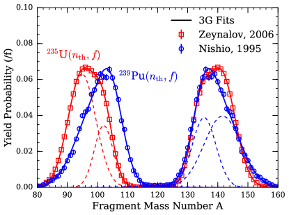
Figure 1: The three-Gaussian parameterization (Eq. 1) is used to fit two experimental mass yields. The squares are for ${}^{235}\mathrm{U}(n_{\mathrm{th}},f)$ from Ref. Zeynalov et al. (2006) and the circles are for ${}^{239}\mathrm{Pu}(n_{\mathrm{th}},f)$ from Ref. Nishio et al. (1995). The dashed lines are the individual Gaussians and the solid curves are the full three-Gaussian fit.

for both the ${}^{235}\mathrm{U}(n_{\mathrm{th}},f)$ reaction Zeynalov et al. (2006) and the ${}^{239}\mathrm{Pu}(n_{\mathrm{th}},f)$ reaction Nishio et al. (1995). We note that the three-Gaussian parameterization is a smooth fit, so it cannot include shell effects. Nevertheless, this parameterization captures the major aspects of the mass yields, so we use it as the input mass yields in the de-excitation calculations.

II.2 Fragment De-excitation

The fragment de-excitation process is calculated in the statistical decay theory of Hauser and Feshbach Hauser and Feshbach (1952). In this formalism, the probabilities for neutron and $\gamma$-ray emission from the excited fragments are calculated at each stage of the decay. These probabilities are derived from the transmission coefficients and level densities via

$$\begin{split}&P(\epsilon_{n})d\epsilon_{n}\propto T_{n}(\epsilon_{n})\rho(A-1,Z,E-\epsilon_{n}-S_{n})d\epsilon_{n}\\ &P(\epsilon_{\gamma})d\epsilon_{\gamma}\propto T_{\gamma}(\epsilon_{\gamma})\rho(A,Z,E-\epsilon_{\gamma})d\epsilon_{\gamma},\end{split}$$ (2)

where the neutron transmission coefficients $T_{n}$ are computed using an optical model with the global optical potential of Koning and Delaroche Koning and Delaroche (2003). The $\gamma$-ray transmission coefficients $T_{\gamma}$ come from the strength functions in the Kopecky-Uhl formalism Kopecky and Uhl (1990) for the different multipolarities considered. The values for the strength-function parameters are taken from the Reference Input Parameter Library (RIPL-3) Capote et al. (2009). The level densities $\rho$ are functions of the fragment mass $A$, charge $Z$, and excitation energy $E$ of the final nuclear state. They are calculated in the Gilbert-Cameron formalism Gilbert and Cameron (1965), where the low excitation energy discrete states are used to create a constant temperature model that connects smoothly to the higher excitation energy continuum states in a Fermi-gas model. Here, $S_{n}$ is the neutron separation energy of a fragment with $Z$ protons and $A$ nucleons. Thus, with Eq. 2, one can determine the probability for a given fragment with excitation energy $E$ to emit either a neutron with energy $\epsilon_{n}$ or a $\gamma$ ray with energy $\epsilon_{\gamma}$. In the Monte Carlo implementation of the Hauser-Feshbach statistical theory Becker et al. (2013), the probabilities are sampled at each step of the de-excitation until the fragments reach a long-lived isomer or their ground state. This is done for many fission events resulting in a large data set, where the energy, spin, and parity are conserved on an event-by-event basis.

To initiate the Hauser-Feshbach decay simulation, one must identify the initial pre-neutron emission fragment distribution and the excitation energy, spin, and parity distributions. The mass $A$, charge $Z$, and total kinetic energy $\mathrm{TKE}$ distribution $Y(A,Z,\mathrm{TKE})$ is sampled to acquire the initial fragment characteristics of a particular fission event. The total excitation energy $\mathrm{TXE}$ between the two complementary fragments is then

$$\begin{split}\mathrm{TXE}=[E_{n}&+B_{n}+M(A_{0},Z_{0})\\ &-M(A_{l},Z_{l})-M(A_{h},Z_{h})]-\mathrm{TKE}(A_{h})\end{split}$$ (3)

where $l$ and $h$ denote the light and heavy fragment, respectively. The mass and charge of the fissioning nucleus is $A_{0}$ and $Z_{0}$ and, in the case of neutron-induced fission, $E_{n}$ is the incident neutron energy and $B_{n}$ is the binding energy of the target. Thus, the first term on the right-hand side in Eq. 3, represents the Q-value of the reaction, with $M(A,Z)$ being the mass of a nucleus with mass number $A$ and charge $Z$.

Next, the $\mathrm{TXE}$ is shared between the two fragments. There are several proposed methods of doing this Litaize and Serot (2010); Schmidt and Jurado (2010, 2011) and the choice of method can dramatically affect some fission observables, particularly the average prompt neutron multiplicity as a function of the fragment mass $\bar{\nu}(A)$ Stetcu et al. (2014); Tudora et al. (2015). We use the $\mathtt{CGMF}$ code Talou et al. (2013b), which is described in Ref. Kawano et al. (2010); Becker et al. (2013), to perform the Monte Carlo treatment of the Hauser-Feshbach decay. The TXE is shared via a ratio of nuclear temperatures $R_{T}$ with

$$R_{T}^{2}=\frac{T_{l}^{2}}{T_{h}^{2}}\approx\frac{E_{l}a_{h}}{E_{h}a_{l}},$$ (4)

where the approximation assumes a Fermi-gas model for the level density to relate the energy $E_{i}$ to the level-density parameter $a_{i}$ and the temperature $T_{i}$. With $\mathrm{TXE}=E_{l}+E_{h}$ and rearranging Eq. 4, we have

$$E_{h}=\mathrm{TXE}\frac{a_{h}}{R_{T}^{2}a_{l}+a_{h}}.$$ (5)

The level density parameters depend on the excitation energy of the corresponding fragments $a_{i}\equiv a_{i}(E_{i})$, so we iteratively solve the right-hand side of Eq. 5 with a given $E_{l}$ and $E_{h}$ and corresponding $a_{l}$ and $a_{h}$, then adjust $E_{l}$ and $E_{h}$ until the chosen $R_{T}$ value is satisfied. In general, $R_{T}$ can have a mass dependence: $R_{T}\equiv R_{T}(A)$. While adjusting $R_{T}(A)$ in order to reproduce the experimental $\bar{\nu}(A)$, we have found that it has little impact on our results.

One key ingredient for the simulation is the initial spin distribution of the fission fragments. As the Hauser-Feshbach model conserves angular momentum, the spin and parity are needed in order to match levels through $\gamma$-ray emission of different multipolarities. Currently, E1, M1, and E2 transitions are considered in $\mathtt{CGMF}$. The spin $J$ distribution follows a Gaussian form

$$P(J)\propto(2J+1)\exp\bigg{[}\frac{-J(J+1)\hbar^{2}}{2\alpha T\mathcal{I}_{0}(A,Z)}\bigg{]},$$ (6)

where $T$ is the nuclear temperature determined from the level density parameter $a$ and the excitation energy $E$. The term $\mathcal{I}_{0}(A,Z)$ is the moment of inertia for a rigid rotor of the ground-state shape of a fragment with a particular mass and charge. The factor $\alpha$ is a spin-scaling factor, which can be used to adjust the average spin of the fragments Kawano et al. (2013). Previous studies have shown that $\alpha$ has a significant effect on the average prompt $\gamma$-ray multiplicity and energy spectrum Stetcu et al. (2014), as well as the isomer production ratios Stetcu et al. (2013). In short, increasing the $J$ of the fragments means more $\gamma$-ray emission at the expense of neutron emission. These additional $\gamma$ rays are usually dipole transitions in the continuum region and low in energy. Thus, an increase in $\alpha$ increases $\mkern 1.5mu\overline{\mkern-1.5muM\mkern-1.5mu}\mkern 1.5mu_{\gamma}$ and softens the overall $\gamma$-ray spectrum. The additional $\gamma$ rays in the continuum lead to a slightly lower prompt neutron multiplicity as well. For this work, we assume equal probability for positive and negative parity in the level density representation of the continuum in the fission fragments, i.e. $P(\pi)=1/2$.

Figure 2: (a) The pre-neutron-emission mass yields $Y(A)$ for ${}^{235}\mathrm{U}(n_{\mathrm{th}},f)$ from the various data sources in the $3$-Gaussian parameterization. The colors correspond to the data source. The thick magenta (red) line is the result of the theoretical calculation by Möller (Sierk) with a $\Delta A=6.0\,\mathrm{u}$ mass resolution. (b) The charge yields $Y(Z)$ from the various input $Y(A)$ folded with Wahl’s Wahl (2002) $Y(Z|A)$. The dotted line uses the $Y(Z|A)$ of Möller Möller and Ichikawa (2015). Black points are the data of Lang et al. Lang et al. (1980).

III Calculations

In the past, the de-excitation calculations have sampled from experimental measurements of the mass yields $Y(A)$, or simple parameterizations Vogt et al. (2009); Becker et al. (2013). In this work, we explore the effect on the fission observables from using the calculated yields described in Sec. II.1 from Ref. Möller and Ichikawa (2015); Sierk (2017). Our procedure is straightforward: we conduct the Hauser-Feshbach decay calculations using $\mathtt{CGMF}$ with different input $Y(A)$ for ${}^{235}\mathrm{U}(n_{\mathrm{th}},f)$ and ${}^{239}\mathrm{Pu}(n_{\mathrm{th}},f)$, both of which have a variety of experimental data available for $Y(A)$ and the various fission observables and correlations. We perform the calculations with the experimental $Y_{e}(A)$ and with the calculated $Y_{c}(A)$ to determine if there are noticeable effects on the observables. This sensitivity study is a first step towards determining the predictive capabilities of the calculated fission yields and developing a fully theoretical and consistent fission model. For this work, we only study the impact of using the calculated mass yields, and leave the prospect of using a two-dimensional $Y(A,Z)$ from Ref. Möller and Ichikawa (2015) or a $Y(A,\mathrm{TKE})$ from Ref. Sierk (2017) for a future study.

For ${}^{235}\mathrm{U}(n_{\mathrm{th}},f)$, we take experimental mass yields $Y_{e}(A)$ from various data sources Dyachenko et al. (1969); Straede et al. (1987); Simon et al. (1990); Baba et al. (1997); Zeynalov et al. (2006) and the two calculated mass yields $Y_{c}(A)$ from Möller Möller and Ichikawa (2015) and Sierk Sierk (2017). For ${}^{239}\mathrm{Pu}(n_{\mathrm{th}},f)$, we take $Y_{e}(A)$ from Ref. Wagemans et al. (1984); Schillebeeckx et al. (1992); Nishio et al. (1995); Tsuchiya et al. (2000) and the $Y_{c}(A)$ from Möller Möller and Ichikawa (2015) and Sierk Sierk (2017). We use multiple $Y_{e}(A)$ in order to determine an uncertainty on the predicted prompt fission observables simply due to the different input experimental mass yields, which is then compared to the values obtained with $Y_{c}(A)$. Input beyond $Y(A)$ are needed to conduct a $\mathtt{CGMF}$ calculation. The calculations require a distribution of fragment charge for a given mass $Y(Z|A)$, which is taken from the Wahl systematics Wahl (2002). One also needs the average $\mathrm{TKE}$ as a function of the fragment mass $\langle\mathrm{TKE}\rangle(A)$, which we take from Ref. Dyachenko et al. (1969) and Ref. Wagemans et al. (1984) for ${}^{235}\mathrm{U}(n_{\mathrm{th}},f)$ and ${}^{239}\mathrm{Pu}(n_{\mathrm{th}},f)$, respectively. The $R_{T}(A)$ are deduced in order to best fit $\bar{\nu}(A)$ from Ref. Vorobyev, A.S. et al. (2010) for ${}^{235}\mathrm{U}(n_{\mathrm{th}},f)$ and from Ref. Apalin et al. (1965) for ${}^{239}\mathrm{Pu}(n_{\mathrm{th}},f)$. The $\alpha$ values are chosen to obtain a reasonable agreement with the $\gamma$-ray multiplicity distributions of Ref. Chyzh et al. (2014) and the average $\gamma$-ray multiplicity $\mkern 1.5mu\overline{\mkern-1.5muM\mkern-1.5mu}\mkern 1.5mu_{\gamma}$ of Ref. Chyzh et al. (2014); Oberstedt et al. (2013); Gatera et al. (2017). The total integrated $\mathrm{TKE}$ is allowed to scale by a factor $\eta$

$$\langle\mathrm{TKE}\rangle=\eta\displaystyle\sum_{A}\langle\mathrm{TKE}\rangle(A)\times Y(A),$$ (7)

where the sum is over the heavy fragment masses. In our analyses, $\eta$ will be given some value to scale the calculated $\bar{\nu}$. Typical values for $\eta$ are within $0.5\%$ of unity. While experimental $\langle\mathrm{TKE}\rangle$ uncertainties are typically reported as less than $200\,\mathrm{keV}$, these uncertainties are only statistical and the systematic uncertainties can be closer to $0.6\%$, or $0.5-1.0\,\mathrm{MeV}$ Milton and Fraser (1962); Wagemans (1991); Nishio et al. (1995). Thus, while the shape of the $\langle\mathrm{TKE}\rangle(A)$ distribution is relatively well-constrained, one can scale the absolute value more freely. The $\mathrm{TKE}$ for a particular fission event is sampled from a Gaussian with mean $\langle\mathrm{TKE}\rangle(A)$ and variance $\sigma^{2}_{\mathrm{TKE}}(A)$, which is taken from Ref. Zakharova et al. (1973) for ${}^{235}\mathrm{U}(n_{\mathrm{th}},f)$. For ${}^{239}\mathrm{Pu}(n_{\mathrm{th}},f)$, we use the shape in Ref. Schillebeeckx et al. (1992) for ²⁴⁰Pu(sf). All $\mathtt{CGMF}$ calculations in this study contain a total of $640000$ fission events.

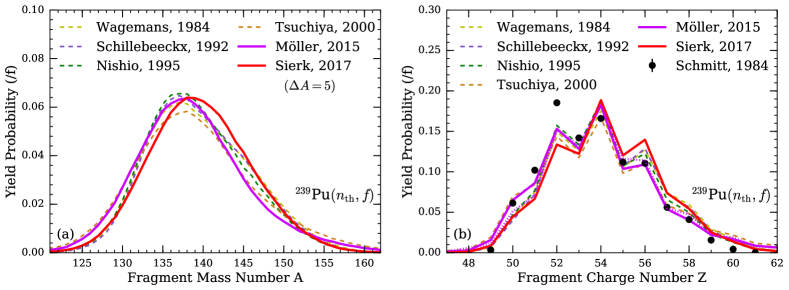
Figure 3: (a) The pre-neutron-emission mass yields $Y(A)$ for ${}^{239}\mathrm{Pu}(n_{\mathrm{th}},f)$ from the various data sources in the $3$-Gaussian parameterization. The colors correspond to the data source. The thick magenta (red) line is the result of the theoretical calculation by Möller (Sierk) with a $\Delta A=5.0\,\mathrm{u}$ mass resolution. (b) The charge yields $Y(Z)$ from the various input $Y(A)$ folded with Wahl’s Wahl (2002) $Y(Z|A)$. The dotted line uses the $Y(Z|A)$ of Möller Möller and Ichikawa (2015). Black points are the data of Schmitt et al. Schmitt et al. (1984) using the $Y(A)$ of Ref. Schillebeeckx et al. (1992) as the normalization of the fractional independent yields.

	Input $Y(A)$	$\langle A_{h}\rangle$ (u)	$\sigma^{2}_{A_{h}}$ (u2)	$\bar{\nu}$ ($n/f$)	$\langle\nu(\nu-1)\rangle$	$\langle\nu(\nu-1)(\nu-2)\rangle$	$\bar{\epsilon}_{n}^{\mathrm{LAB}}$ (MeV)	$\mkern 1.5mu\overline{\mkern-1.5muM\mkern-1.5mu}\mkern 1.5mu_{\gamma}$ ($\gamma/f$)	$\bar{\epsilon}_{\gamma}$ (MeV)
${}^{235}\mathrm{U}(n_{\mathrm{th}},f)$	Dyachenko Dyachenko et al. (1969)	139.16	28.69	2.458	4.766	6.749	1.984	7.284	0.856
	Straede Straede et al. (1987)	139.50	27.27	2.423	4.620	6.390	1.974	7.308	0.851
	Simon Simon et al. (1990)	139.74	30.59	2.382	4.457	6.020	1.967	7.311	0.852
	Baba Baba et al. (1997)	139.00	32.88	2.458	4.772	6.783	1.988	7.274	0.860
	Zeynalov Zeynalov et al. (2006)	139.17	28.63	2.454	4.751	6.710	1.983	7.294	0.855
	Möller Möller and Ichikawa (2015)	137.39	33.57	2.621	5.485	8.618	2.029	7.189	0.876
	Sierk Sierk (2017)	139.73	31.47	2.373	4.438	6.034	1.963	7.313	0.850
ENDF/B-VIII.0 Brown et al.				2.414$\pm$0.01	4.641	6.716	2.00$\pm$0.01	8.19	0.89
${}^{239}\mathrm{Pu}(n_{\mathrm{th}},f)$	Wagemans Wagemans et al. (1984)	139.67	41.86	2.887	6.766	12.13	1.998	7.711	0.864
	Schillebeeckx Schillebeeckx et al. (1992)	139.61	39.65	2.901	6.828	12.31	2.001	7.715	0.863
	Nishio Nishio et al. (1995)	139.13	38.77	2.948	7.058	12.97	2.017	7.695	0.867
	Tsuchiya Tsuchiya et al. (2000)	139.21	57.48	2.875	6.711	12.00	2.001	7.668	0.877
	Möller Möller and Ichikawa (2015)	138.82	48.53	2.955	7.097	13.11	2.019	7.658	0.876
	Sierk Sierk (2017)	139.68	38.90	2.888	6.777	12.18	1.994	7.742	0.860
ENDF/B-VIII.0 Brown et al.				2.870$\pm$0.01	6.721	12.51	2.117$\pm$0.037	7.33	0.87

Table 1: Average quantities for $\mathtt{CGMF}$ calculations utilizing different mass yields for ${}^{235}\mathrm{U}(n_{\mathrm{th}},f)$ and ${}^{239}\mathrm{Pu}(n_{\mathrm{th}},f)$. These calculations used $\langle\mathrm{TKE}\rangle=171.40\,\mathrm{MeV}$ for ${}^{235}\mathrm{U}(n_{\mathrm{th}},f)$ Nishio et al. (1998) and $\langle\mathrm{TKE}\rangle=177.93\,\mathrm{MeV}$ for ${}^{239}\mathrm{Pu}(n_{\mathrm{th}},f)$ Schillebeeckx et al. (1992). Listed are the average heavy-fragment mass $\langle A_{h}\rangle$, the heavy-fragment peak variance $\sigma^{2}_{A_{h}}$, the average prompt neutron multiplicity $\bar{\nu}$, its first $\langle\nu(\nu-1)\rangle$ and second $\langle\nu(\nu-1)(\nu-2)\rangle$ factorial moments, the average prompt neutron energy in the lab frame $\bar{\epsilon}_{n}^{\mathrm{LAB}}$, the average prompt $\gamma$-ray multiplicity $\mkern 1.5mu\overline{\mkern-1.5muM\mkern-1.5mu}\mkern 1.5mu_{\gamma}$, and average $\gamma$-ray energy $\bar{\epsilon}_{\gamma}$. The calculations used an energy threshold of $\epsilon_{n}^{\mathrm{LAB}}>10\,\mathrm{keV}$ and $\epsilon_{\gamma}>100\,\mathrm{keV}$, as well as a timing window of $\Delta t=10\,\mathrm{ns}$ for the $\gamma$ rays. Values from ENDF/B-VIII.0 Brown et al. are also listed with similar detection thresholds.

Pre-neutron-emission fragment mass and charge yields are presented in Fig. 2 for ${}^{235}\mathrm{U}(n_{\mathrm{th}},f)$ and in Fig. 3 for ${}^{239}\mathrm{Pu}(n_{\mathrm{th}},f)$. The dashed lines are the three-Gaussian parameterizations for the different $Y_{e}(A)$. The thick solid lines are the three-Gaussian parameterizations for the two $Y_{c}(A)$. We note that the calculated yields $Y_{c}(A)$ Möller and Ichikawa (2015); Sierk (2017) have been folded with a mass resolution of $\Delta A\sim 6\,\mathrm{u}$ at FWHM. The resulting charge yields $Y(Z)$ are also given for each reaction. Recall that the $Y(Z|A)$ are from Wahl Wahl (2002), but the differences in the $Y(A)$ are propagated to the resulting $Y(Z)$, where we see that the spread in the $Y(Z)$ is directly correlated to that in $Y(A)$. For example, the increase between $125\leq A\leq 135$ for ${}^{235}\mathrm{U}(n_{\mathrm{th}},f)$ in the $Y_{c}(A)$ of Ref. Möller and Ichikawa (2015) is accompanied by an increase in the charge yields around $49\leq Z\leq 51$. The same trends are found in Fig. 3 for ${}^{239}\mathrm{Pu}(n_{\mathrm{th}},f)$.

An important feature of the fragment mass yields is the average heavy fragment mass $\langle A_{h}\rangle$. From Eq. 7, one can see that masses with the largest yields, i.e. those near $\langle A_{h}\rangle$, will dominate the sum and determine the $\langle\mathrm{TKE}\rangle$ to first order. The input $\langle\mathrm{TKE}\rangle(A)$ of Ref. Dyachenko et al. (1969) and Ref. Wagemans et al. (1984) both peak near $A=132$. Thus, mass yields with large $Y(A\sim 132)$ will result in the largest $\langle\mathrm{TKE}\rangle$. From Eq. 3, we note that a larger $\langle\mathrm{TKE}\rangle$ results in a lower $\langle\mathrm{TXE}\rangle$, which provides less energy for the prompt neutron and $\gamma$-ray emissions. In addition, a different set of mass yields will generate a change in the $Q$-value for the fission reaction as the fragment masses are different. For our calculations, we have either fixed the $\langle\mathrm{TKE}\rangle$ to be $171.40\,\mathrm{MeV}$ Nishio et al. (1998) for ${}^{235}\mathrm{U}(n_{\mathrm{th}},f)$ and $177.93\,\mathrm{MeV}$ Schillebeeckx et al. (1992) for ${}^{239}\mathrm{Pu}(n_{\mathrm{th}},f)$, or allowed the $\langle\mathrm{TKE}\rangle$ value to float but restrict $\bar{\nu}$ to be in agreement with the IAEA standards Carlson et al. (2009): $2.419\,n/f$ for ${}^{235}\mathrm{U}(n_{\mathrm{th}},f)$ and $2.877\,n/f$ for ${}^{239}\mathrm{Pu}(n_{\mathrm{th}},f)$.

As seen in Table 1, the changes in the mass yields can translate to a change in prompt fission observables. For these $\mathtt{CGMF}$ calculations, we used a fixed $\langle\mathrm{TKE}\rangle$, which means that the $\eta$ values are different for each choice of $Y(A)$ via Eq. 7. This change in $\eta$ shifts the $\langle\mathrm{TKE}\rangle(A)$, which shifts the $\langle\mathrm{TXE}\rangle(A)$ in the opposite direction. Thus, lower $\eta$ values will increase $\langle\mathrm{TXE}\rangle(A)$ and result in a larger $\bar{\nu}$ for the fission reaction, as the excitation energy is

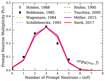
Figure 4: The prompt neutron multiplicity distribution $P(\nu)$ of ${}^{239}\mathrm{Pu}(n_{\mathrm{th}},f)$ for the various input experimental $Y_{e}(A)$ (dashed lines) or calculated $Y_{c}(A)$ (thick solid lines). Black points are the data of Boldeman Boldeman and Hines (1985) and Holden Holden and Zucker (1988).

largely removed by neutron emission Talou et al. (2016). Assuming $5\,\mathrm{MeV}/n$ from averaging over all fragments, the statistical differences in the $\langle\mathrm{TKE}\rangle$ values for the calculations in Table 1 could only account for a difference of $0.4\%$ in $\bar{\nu}$. However, we find that the different $Y(A)$ can produce up to a $7.7\%$ change in $\bar{\nu}$ and a $1.2\%$ change in $\mkern 1.5mu\overline{\mkern-1.5muM\mkern-1.5mu}\mkern 1.5mu_{\gamma}$. This change in $\mkern 1.5mu\overline{\mkern-1.5muM\mkern-1.5mu}\mkern 1.5mu_{\gamma}$ is relatively small, compared with the experimental uncertainties Chyzh et al. (2014); Oberstedt et al. (2013); Gatera et al. (2017) and could be solely caused by the correlation between $\bar{\nu}$ and $\mkern 1.5mu\overline{\mkern-1.5muM\mkern-1.5mu}\mkern 1.5mu_{\gamma}$ Wang et al. (2016), i.e. that the change in $\mkern 1.5mu\overline{\mkern-1.5muM\mkern-1.5mu}\mkern 1.5mu_{\gamma}$ is only indirectly related to the change in $Y(A)$ through the change in $\bar{\nu}$. The differences in $\bar{\nu}$, however, are $1-8\%$, about an order of magnitude larger than the experimental uncertainties Boldeman and Hines (1985); Holden and Zucker (1988). This indicates that $\bar{\nu}$ can be very sensitive to the choice of $Y(A)$. The overall trend in Table 1 is that a $Y(A)$ with $\langle A_{h}\rangle$ closer to $132$ will result in a lower $\eta$ to maintain a fixed $\langle\mathrm{TKE}\rangle$. This will then increase $\langle\mathrm{TXE}\rangle$ and produce more prompt neutrons. Figure 4 demonstrates this point for ${}^{239}\mathrm{Pu}(n_{\mathrm{th}},f)$. We note that the factorial moments of $P(\nu)$ are very sensitive to the variance $\sigma^{2}_{\mathrm{TKE}}(A)$. A scaling of $\sigma^{2}_{\mathrm{TKE}}(A)$ by $0.76$ for ${}^{235}\mathrm{U}(n_{\mathrm{th}},f)$ and $0.81$ for ${}^{239}\mathrm{Pu}(n_{\mathrm{th}},f)$ was used to obtain reasonable agreement with the experimental $P(\nu)$ Boldeman and Hines (1985); Holden and Zucker (1988). All calculations shown in this work use the same $\sigma^{2}_{\mathrm{TKE}}(A)$ and the same scaling, meaning that the changes in $P(\nu)$ seen in Fig. 4 are a direct result of the change in $Y(A)$ only.

Figure 5: The correlation between the average total kinetic energy of the fragments $\langle\mathrm{TKE}\rangle$ and the average prompt neutron multiplicity $\bar{\nu}$ for ${}^{235}\mathrm{U}(n_{\mathrm{th}},f)$ (bottom) and ${}^{239}\mathrm{Pu}(n_{\mathrm{th}},f)$ (top). The calculations have either a fixed $\langle\mathrm{TKE}\rangle$ (circles) or a fixed $\bar{\nu}$ (triangles). Horizontal lines are the experimental $\langle\mathrm{TKE}\rangle$ for ${}^{235}\mathrm{U}(n_{\mathrm{th}},f)$ Nishio et al. (1998) and ${}^{239}\mathrm{Pu}(n_{\mathrm{th}},f)$ Schillebeeckx et al. (1992) with the shaded regions representing $\pm 0.5\,\mathrm{MeV}$ (dashed darker region) and $\pm 1.0\,\mathrm{MeV}$ (dotted lighter region). Vertical lines are the evaluated $\bar{\nu}$ and their $1\sigma$ (dashed darker region) and $3\sigma$ (dotted lighter region) uncertainty bands Carlson et al. (2009).

From our initial calculations, we can already see that differences in $Y(A)$ can produce changes in $\bar{\nu}$ above the sub-percent reported uncertainties for both ${}^{235}\mathrm{U}(n_{\mathrm{th}},f)$ and ${}^{239}\mathrm{Pu}(n_{\mathrm{th}},f)$ evaluated by the standards group Carlson et al. (2009). We can invert the procedure to instead fix $\bar{\nu}$ to the evaluated values and determine the corresponding $\langle\mathrm{TKE}\rangle$ value needed. This procedure, and its comparison with the method of fixing $\langle\mathrm{TKE}\rangle$, is shown in Fig. 5. The different $Y(A)$ induce typical errors of $\delta\langle\mathrm{TKE}\rangle\sim 0.4\%$ and $\delta\bar{\nu}\sim 4\%$. One intriguing result from this study is that a highly precise measurement of $\bar{\nu}$ could be used to constrain the allowed values for $\langle\mathrm{TKE}\rangle$, as already mentioned in Ref. Randrup et al. (2017). In the bottom plot of Fig. 5, when we fix $\bar{\nu}$ to the evaluated value, the spread in $\langle\mathrm{TKE}\rangle$ values induced from the choice of $Y(A)$ is within the $\pm 0.5\,\mathrm{MeV}$ range. This implies that the experimental uncertainty on $\langle\mathrm{TKE}\rangle$, $1.4\,\mathrm{MeV}$ in Ref. Nishio et al. (1998) could be reduced by the constraints on $\bar{\nu}$ by about a factor of $3$. The differences in the input mass yields seem to limit this type of correlation analysis to about $\pm 0.4\,\mathrm{MeV}$ in the $\langle\mathrm{TKE}\rangle$ uncertainties. We note that the average spin of the fragments, governed by $\alpha$, and the shape of $\langle\mathrm{TKE}\rangle(A)$ will also influence the correlation between $\langle\mathrm{TKE}\rangle$ and $\bar{\nu}$.

The changes in the prompt fission neutron (PFNS) and prompt fission $\gamma$-ray (PFGS) spectra are shown in Fig. 6 and Fig. 7.

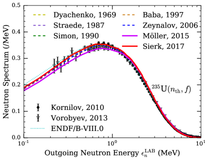
Figure 6: The prompt fission neutron energy spectrum (PFNS) of ${}^{235}\mathrm{U}(n_{\mathrm{th}},f)$ in the lab frame calculated with the various input experimental $Y_{e}(A)$ (dashed lines) or calculated $Y_{c}(A)$ (thick solid lines). Black points are the data of Kornilov et al. Kornilov et al. (2010) and Vorobyev et al. Capote et al. (2016). The dotted line is from ENDF/B-VIII.0 Brown et al. .

The PFNS is plotted to illustrate the impact of the different $Y(A)$ at low outgoing neutron energies. We can see that mass yields shifted closer to symmetry will have a slightly harder PFNS, as the average neutron energies are larger for these masses Göök et al. (2014); Nishio et al. (1998); Tsuchiya et al. (2000). Even with this shift, the typical error on the average outgoing neutron energy from using calculated mass yields is $\delta\bar{\epsilon}_{n}^{\mathrm{LAB}}\sim 1\%$. Overall, the PFNS is mostly insensitive to the choice of input $Y(A)$. An additional note is that the PFNS calculated by $\mathtt{CGMF}$ are consistently softer than the experimental ones for neutron energies above $4\,\mathrm{MeV}$, an issue also identified in previous studies Becker et al. (2013); Kawano et al. (2013). This work demonstrates that the choice of input mass yields does not seem to account for this discrepancy.

The PFGS in Fig. 7 also appears relatively insensitive to the choice of input $Y(A)$. We note that the calculation of ${}^{235}\mathrm{U}(n_{\mathrm{th}},f)$ using the $Y(A)$ from Möller Möller and Ichikawa (2015) produces a slightly harder PFGS as the mass yields are more shifted towards the $N=82$ closed shell, where the average $\gamma$-ray energy is known to peak Pleasonton et al. (1972); Hotzel et al. (1987) due to the large level spacing. A similar argument reveals why the average $\gamma$-ray energy for the Tsuchiya et al. Tsuchiya et al. (2000) mass yields is relatively large. Even though its average heavy fragment peak is not the closest to $A=132$, the peak width is large enough to produce larger yields for $A\sim 132$ than the other input yields, as seen in Fig. 3. Thus, both $\langle A_{h}\rangle$ and $\sigma^{2}_{A_{h}}$ can impact the prompt fission observables. We note that specific $\gamma$-ray lines are sensitive to the choice of input mass yields, as seen in the insert in Fig. 7. For example, the $212.53\,\mathrm{keV}$ peak of ¹⁰⁰Zr is $5\%$ more intense with the $Y_{c}(A)$ of Möller Möller and Ichikawa (2015) instead of Sierk Sierk (2017), due to the change in peak location seen in Fig. 2. Overall, typical errors of $\delta\bar{\epsilon}_{\gamma}\sim 1\%$ occur when using the calculated yields over experimental ones. We note that recent studies involving significantly different

Figure 7: The prompt fission $\gamma$-ray energy spectrum (PFGS) of ${}^{235}\mathrm{U}(n_{\mathrm{th}},f)$ calculated with the various input experimental $Y_{e}(A)$ (dashed lines) or calculated $Y_{c}(A)$ (thick solid lines). Black points are the data of Oberstedt et al. Oberstedt et al. (2013) and Chyzh et al. Chyzh et al. (2014). We use an energy threshold of $100\,\mathrm{keV}$ and a timing window of $10\,\mathrm{ns}$ in accordance with Ref. Oberstedt et al. (2013). The dotted line is from ENDF/B-VIII.0 Brown et al. . Insert shows the low-energy region.

mass yields, such as those between spontaneous fission and neutron-induced fission from the same compound nucleus, can generate a measurable difference in the PFGS Chyzh et al. . In Fig. 7, the calculated spectra deviate from the experimental data above $\epsilon_{\gamma}=5\,\mathrm{MeV}$, with the $\mathtt{CGMF}$ calculations underpredicting the measured spectrum. Previous studies Stetcu et al. (2013, 2014) have demonstrated that decreasing the spin-scaling factor $\alpha$ can increase the slope of the PFGS, but this will lower $\mkern 1.5mu\overline{\mkern-1.5muM\mkern-1.5mu}\mkern 1.5mu_{\gamma}$, creating tension with the values of Ref. Oberstedt et al. (2013); Chyzh et al. (2014); Gatera et al. (2017).

We now turn to the correlation between the total kinetic energy and the total number of prompt neutrons emitted from both the light and heavy fragment $\bar{\nu}_{T}$. This relation utilizes the energy conservation in Eq. 3 and is expected to be anti-correlated as a larger $\mathrm{TKE}$ results in less energy available for prompt neutron emission. In Fig. 8, this trend is seen by the decreasing trend of $\bar{\nu}_{T}(\mathrm{TKE})$ for ${}^{235}\mathrm{U}(n_{\mathrm{th}},f)$. The $\mathtt{CGMF}$ calculations reproduce the experimental data of Göök et al. Göök et al. (2017) very well. A possible explanation for the differences seen for $\mathrm{TKE}>180\,\mathrm{MeV}$ is a broader $\mathrm{TKE}$ resolution in Boldeman et al. Boldeman et al. (1971). The $\mathrm{TKE}$ bins below $140\,\mathrm{MeV}$ have poor statistics in the $\mathtt{CGMF}$ calculations, so we have cut the calculated curves at this value. We note two trends seen in Fig. 8. First, mass yields with a lower $\langle A_{h}\rangle$ require a lower $\eta$ to keep $\langle\mathrm{TKE}\rangle$ fixed, which results in more excitation energy available for the fragments and a shift towards higher $\bar{\nu}_{T}(\mathrm{TKE})$. Second, mass yields with wider peaks (larger $\sigma^{2}_{A_{h}}$) result in a shallower slope for the $\mathrm{TKE}<160\,\mathrm{MeV}$ bins. For example, the result using $Y_{e}(A)$ from Baba et al. Baba et al. (1997) is very similar to the result when using $Y_{e}(A)$ from Ref. Dyachenko et al. (1969); Straede et al. (1987); Zeynalov et al. (2006) for $\mathrm{TKE}>160\,\mathrm{MeV}$, but becomes closer to the result using $Y_{c}(A)$ from Sierk Sierk (2017) for $\mathrm{TKE}<160\,\mathrm{MeV}$. When we take a single $Y(A)$ and arbitrarily add a mass resolution, which keeps $\langle A_{h}\rangle$ about constant while increasing $\sigma^{2}_{A_{h}}$, we find the same trend.

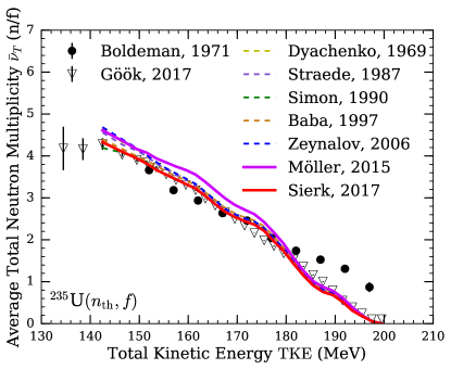
Figure 8: The correlation between the total kinetic energy of the fission fragments and the average total prompt neutron multiplicity between both the light and heavy fragments $\bar{\nu}_{T}(\mathrm{TKE})$ of ${}^{235}\mathrm{U}(n_{\mathrm{th}},f)$ for various input experimental $Y_{e}(A)$ (dashed lines) or calculated $Y_{c}(A)$ (thick solid lines). Black points are the data from Boldeman et al. Boldeman et al. (1971) and Göök et al. Göök et al. (2017).

This occurs because a larger $\sigma^{2}_{A_{h}}$ introduces a wider variety of mass yields contributing to the same $\mathrm{TKE}$ energy bin. In particular, for the lower $\mathrm{TKE}$ energy bins, the contribution of very asymmetric yields increases, which also tend to have a low $\bar{\nu}_{T}$ Vorobyev, A.S. et al. (2010). This additional influence of very asymmetric mass splits lowers the $\bar{\nu}_{T}$ for that $\mathrm{TKE}$ energy bin, thus resulting in the trend seen in Fig. 8. This low-$\mathrm{TKE}$ region is difficult for experiments, where correcting for detector effects, such as neutron scattering, capture efficiency, and the recoil imparted onto the fragment, can play a large role Gavron (1974); Nifenecker et al. (1974); Göök et al. (2014); Vorobyev, A.S. et al. (2010). Overall, we find that the shift towards higher $\bar{\nu}_{T}(\mathrm{TKE})$ is primarily due to the different $\langle A_{h}\rangle$, while the change in the slope of $\bar{\nu}_{T}(\mathrm{TKE})$ at low $\mathrm{TKE}$ values is due to the different $\sigma^{2}_{A_{h}}$.

IV Conclusion

We have used theoretical models for the fragment mass yields Möller and Ichikawa (2015); Sierk (2017) as input for Hauser-Feshbach simulations of the emission of prompt neutrons and $\gamma$ rays Becker et al. (2013). This allows us to test the feasibility of using theoretically calculated fission-fragment yields and determine the sensitivity of important prompt fission observables, such as the average prompt neutron multiplicity $\bar{\nu}$, average total kinetic energy of the fragments $\langle\mathrm{TKE}\rangle$, and average energies of the emitted neutrons and $\gamma$ rays, to the input yields. We utilize the ${}^{235}\mathrm{U}(n_{\mathrm{th}},f)$ and ${}^{239}\mathrm{Pu}(n_{\mathrm{th}},f)$ reactions, as there is significant experimental data for both the mass yields $Y(A)$ and prompt fission observables. An initial comparison of the mass yields demonstrates that the calculated yields can achieve reasonable agreement with most experimental data. Using a Monte Carlo implementation of the Hauser-Feshbach statistical decay model Talou et al. (2013b), we propagate the differences between the experimental and calculated mass yields to differences in the prompt neutron and $\gamma$-ray observables. In particular, we find that the average heavy fragment mass $\langle A_{h}\rangle$ is very influential in determining $\langle\mathrm{TKE}\rangle$, which, in turn, is a major factor in determining $\bar{\nu}$. This finding is reflected in Table 2, where we list the correlation between the calculated $\bar{\nu}$ and input $\langle A_{h}\rangle$. The correlation is determined by fitting ordered pairs of $(\langle A_{h}\rangle,\bar{\nu})$ for each set of mass yields in Tab. 1.

	${}^{235}\mathrm{U}(n_{\mathrm{th}},f)$			${}^{239}\mathrm{Pu}(n_{\mathrm{th}},f)$
$\partial\bar{\nu}/\partial\langle A_{h}\rangle$ ($n/f$/u)	$\pm 0.11$			$\pm 0.08$
	Möller Möller and Ichikawa (2015)	Sierk Sierk (2017)	Exp. or Eval.	Möller Möller and Ichikawa (2015)	Sierk Sierk (2017)	Exp. or Eval.
$\delta\langle\mathrm{TKE}\rangle$ (MeV)	$0.8\%$	$0.3\%$	$0.6\%$ Wagemans (1991)	$0.2\%$	$0.1\%$	$0.6\%$ Wagemans (1991)
$\delta\bar{\nu}$ ($n/f$)	$7.7\%$	$2.6\%$	$0.4\%$ Chadwick et al.	$1.8\%$	$0.5\%$	$0.3\%$ Chadwick et al.
$\delta\bar{\epsilon}_{n}^{\mathrm{LAB}}$ (MeV)	$2.5\%$	$0.8\%$	$0.5\%$ Capote et al. (2016)	$0.7\%$	$0.5\%$	$1.7\%$ Neudecker et al.
$\delta\mkern 1.5mu\overline{\mkern-1.5muM\mkern-1.5mu}\mkern 1.5mu_{\gamma}$ ($\gamma/f$)	$1.2\%$	$0.5\%$	$1.3\%$ Oberstedt et al. (2013)	$0.3\%$	$0.3\%$	$1.6\%$ Gatera et al. (2017)
$\delta\bar{\epsilon}_{\gamma}$ (MeV)	$2.1\%$	$0.9\%$	$2.4\%$ Oberstedt et al. (2013)	$0.8\%$	$0.7\%$	$2.4\%$ Gatera et al. (2017)

Table 2: Correlation between calculated $\bar{\nu}$ and the input average heavy fragment mass $\langle A_{h}\rangle$ for ${}^{235}\mathrm{U}(n_{\mathrm{th}},f)$ and ${}^{239}\mathrm{Pu}(n_{\mathrm{th}},f)$. Also listed are the biases for several prompt fission observables from using calculated mass yields of Möller Möller and Ichikawa (2015), Sierk Sierk (2017), as well as experimental uncertainties for reference.

This correlation implies that, when all other input is kept constant, two mass yields with heavy fragment peaks one mass unit apart will result in a $\bar{\nu}$ differing by about $0.1\,n/f$. Very different peak widths $\sigma_{A_{h}}^{2}$ complicate the correlation. We note that this analysis relies on the shape of the $\langle\mathrm{TKE}\rangle(A)$ we have chosen, but not on the overall $\langle\mathrm{TKE}\rangle$, which only shift the ordered pairs and leave the correlation unaffected.

Also listed in Table 2 are the biases on the various prompt fission observables from the use of calculated yields instead of experimental ones. We find that both the location of the mass peak $\langle A_{h}\rangle$ and the width of the peak $\sigma^{2}_{A_{h}}$, where wider peaks resulting in an increased yield near the $N=82$ shell closure, could result in a slightly harder PFNS and PFGS. Specific discrete $\gamma$-ray intensities are also directly affected by the choice of mass yields. The width of the mass peak was also found to impact the correlation between the total kinetic energy of the fragments and the average total prompt neutron multiplicity.

These correlations and derived biases will help inform future fission-yield models and the de-excitation procedure. These calculations can be improved with self-consistent $Y(A,Z)$ yields from Ref. Möller and Ichikawa (2015) and $Y(A,\mathrm{TKE})$ yields from Ref. Sierk (2017). In a future study, we plan to implement the exact fission-fragment mass yields into the Hauser-Feshbach statistical-decay model and apply the effects of the experimental mass and energy resolutions to the calculated results, instead of applying a mass resolution to the input mass yields. Additional experimental data of the fragment mass, charge, and kinetic energies at a variety of incident neutron energies, such as Refs. Duke et al. (2016); Meierbachtol et al. (2016), would allow for a more critical comparison of the calculated and experimental yields. Furthermore, measurements of the fragment yields for exotic nuclei will improve our ability to benchmark calculated yields outside the more well-studied actinide chains. When calculating the prompt neutron and $\gamma$-ray emissions, several input parameters are needed, but may not possess the proper energy dependence as there is no data available. For example, the dependence of $\langle\mathrm{TKE}\rangle(A)$ on incident neutron energy has only been determined for a limited number of nuclei Duke et al. (2016); Meierbachtol et al. (2016). In addition, properties of the prompt $\gamma$ rays have seldom been measured at higher incident neutron energies Fréhaut et al. (1983), but additional data may provide useful information about the spins of fission fragments at these energies. Finally, measurements conducted by Naqvi et al. Naqvi et al. (1986) demonstrated that $\bar{\nu}(A)$ has a distinct change in shape for higher incident neutron energies, but further experimental tests of this would provide useful insight into the excitation energy sharing in fission.

Our results utilize theoretical methods to calculate fission observables from scission to prompt neutron and $\gamma$-ray emissions, a step towards a predictive model of fission. In general, we find that the use of calculated yields do not yet possess the precision needed for very sensitive criticality estimates Neudecker et al. (2016) or neutron correlation counting Croft et al. (2015). However, it should be noted that the variance on $\bar{\nu}$ induced simply from the differences in the experimental mass yields is already near the uncertainties of the IAEA standards Carlson et al. (2009). For applications that do not require this degree of accuracy, we find that the use of calculated mass yields and the prompt particle emission through a Hauser-Feshbach treatment is invaluable, especially where there is little to no experimental data as is the case in many nuclides participating in the $r$-process Côté et al. (2017). Furthermore, the prompt $\gamma$-ray observables appear less sensitive to the use of calculated mass yields instead of experimental ones, suggesting that estimates of $\gamma$-ray heating for reactor design could be done for nuclides without experimental data using a combination of theoretical mass yields and a Hauser-Feshbach decay treatment, as we have used here, and still satisfy the needed design uncertainties Rimpault et al. (2012).