Experimental design trade-offs for gene regulatory network inference:
an in silico study of the yeast  cell cycle

Abstract

Time-series of high throughput gene sequencing data intended for gene regulatory network (grn) inference are often short due to the high costs of sampling cell systems. Moreover, experimentalists lack a set of quantitative guidelines that prescribe the minimal number of samples required to infer a reliable grn model. We study the temporal resolution of data vs. quality of grn inference in order to ultimately overcome this deficit. The evolution of a Markovian jump process model for the ras/camp/pka pathway of proteins and metabolites in the G₁ phase of the cell cycle is sampled at a number of different rates. For each time-series we infer a linear regression model of the grn using the lasso method. The inferred network topology is evaluated in terms of the area under the precision-recall curve (aupr). By plotting the aupr against the number of samples, we show that the trade-off has a, roughly speaking, sigmoid shape. An optimal number of samples corresponds to values on the ridge of the sigmoid.

I Introduction

Time-series gene expression data provides a series of snapshots of molecular concentrations in gene regulatory networks (grn) [1]. This information is used to infer dynamic models of grn networks which aid our understanding of how observable phenotypes, e.g., diseases, arise from molecular interactions [2]. As such, time-series data is of importance to fundamental research within systems biology, and potentially also in applications like medical diagnostics, drug development, and therapies [3]. The advent of high throughput sequencing have made time-series data widely available although it is prohibitively expensive to densely sample gene expression levels. It remains difficult for experimentalists to accurately judge the frequency and distribution of samples needed to infer network structures: for each project, they must navigate the trade-off between oversampling (more samples than necessary, increasing costs with no benefit to grn inference) and undersampling (too few samples to reliably infer the grn, potential waste of resources and failure to infer the grn) [4]. Such costs add up; studies indicate that 85% of research investment in biomedical sciences is wasted, corrsponding to US$200 billion worldwide in 2010 [5]. This work undertakes an in silico study of the impact of the cost vs. number of samples trade-offs on the quality of the output produced by a grn inference algorithm. Our ultimate goal, to which this paper is a stepping stone, is to formulate guidelines and construct decision support systems to help researches navigate trade-offs such that grn models of desired quality can be inferred at a minimal cost.

The performance of grn inference algorithms has been benchmarked against in silico and in vivo data in a number of comparative studies [6, 7, 8, 9]. The aforementioned trade-off has received comparatively less attention [1, 10, 4, 11, 12]. There are of course many works that touch upon it in passing, e.g., [13], or that pay the price of intentionally oversampling to ensure capturing high-frequency content [14, 15]. Early work that take a systematic approach to studying the trade-off are rather abstracts and deal with generalities in broad strokes [1, 10, 4]. For example, [1] states that cyclic processes such as cell cycles and circadean rythms should be sampled uniformly over multiple cycles. In perturbation-response studies, by contrast, most samples should be taken early to capture the transient dynamics.

Only in the past year have results been published to support the common sense notions of navigating the trade-off that are current experimental practices [11, 12]. Sefer et al. [11] take an in-depth look at the experimental design question of sampling densely versus sampling repeatedly; the former is recommended for the purpose of detecting a spike in the molecule count number of some species. Mombaerts et al. [12] study the difference between transient and steady-state sampling of the circadian clock in Arabidopsis thaliana, finding that the transient contains more information. In a similar vein, this paper establishes that the performance of an inference algorithm that fits a linear model to a pathway in the G₁ phase of the cell cycle is comparable to random classifier in the case of 3–6 samples, increases over 7–11 samples, and then flattens out with additional samples giving diminishing returns. Together with [11], [12], this paper represents a first effort to refine previous, rule based experiment trade-off navigation practices [1, 10, 4], into more specific, quantitative guidelines.

Alongside the development of novel grn inference algorithms, new models have been adopted to generate in silico data and represent the dynamics of inferred networks [16, 17, 18, 19, 20]. grn models exist at different levels of abstraction, from the logical models captured by Boolean networks, over continuous models, e.g., systems of ordinary differential equations, to the mesoscopic single molecule models such as chemical reaction networks (crn) whose dynamics are modeled as Markovian jump processes governed by the chemical master equation (cme) [20]. To measure the performance of a grn inference algorithm, the ground truth in terms of gene expression causal interactions is required. For in vivo data, the ground truth is often unavailable and replacing it with a known gold standard poses certain challenges [10, 21], making in silico studies an attractive alternative [19]. In this paper we require in silico models to generate output with a wide range of sample rates. We strive to replicate realistic experiment conditions, e.g., choosing a detailed in silico model of cellular dynamics based on Markovian jump processes to represent key characteristics such as intrinsic noise [19, 22], common network motifs like sparsity [16, 17], and species with highly different concentrations [23].

This paper uses the cme to model a pathway involved in the G₁ phase of the S. cerevisiae cell cycle [23], following the experiment setup of a query driven rather than a global study [21]. A sample is drawn from the probability density function governed by the cme using a stochastic simulation algorithm (ssa). We then infer a linear autoregressive model to explain the in silico data using the lasso method [24]. lasso provides a basic approach for grn inference [8], and has the benefit of imposing sparsity on the regression parameters, thereby capturing a characteristic grn motif. Large regression coefficients suggest the existence of regulatory interactions between species, whereby an interaction topology can be extracted by thresholding the model parameters. The area under the precision-recall curve is used to score the performance of lasso by comparing the inferred topology with that of the crn simulated by the ssa[25]. We obtain a graph of the trade-off by repeating the inference procedure for data of varying temporal resolution. The main contributions of this paper can be summarized as follows: (i) we establish that the trade-off function which charts performance over number of samples has a sigmoid shape for a pathway in the G₁ phase of the S. cerevisiae cell cycle and the lasso method and (ii) we provide a graph that allows an experimentalist to match a desired quality of inference (for the pathway) with a minimum number of samples.

II Research Question and Research Problem

Suppose that the experiment budget is somewhat flexible, and that there exist incentives to cut costs. Consider how a biologist conducting a high throughput gene sequencing experiment should navigate the number of samples vs. quality of grn inference trade-off. Since the cost of undersampling is an incomplete or failed study whereas oversampling amounts to a waste of resources, we express the multiobjective optimization problem, i.e., the trade-off, in terms of a hard constraint on the quality of the inferred network: minimize the number of samples required to achieve a certain quality of inference for a given experiment, i.e., to optimize marginal costs. For this paper we limit the scope to a particular model of the ras/camp/pka pathway in S. cerevisiae [23] and the lasso method applied to grn inference [24]. Consider the resolution of gene expressions measurements in cases where additional detail can be purchased at a cost that is higher than that of additional samples, i.e., to optimize fixed costs. In particular, we study the cases of including or excluding a phosphoproteomic analysis of S. cerevisiae, which requires the use of different techniques compared to proteomics and metabolomics [26] (the low molecule count numbers for phosphorylated proteins requires a larger cell culture).

III Method

To begin with, in silico data is generated from a Markov process model of a pathway in the yeast S. cerevisiae cell cycle, see Section III-B. To simulate the model, an efficient solver for the chemical master equation is required as detailed in Section III-A. The model of the pathway is from [23], and has been verified against experimental data. The model consists of molecule count numbers for a total of 30 proteins and metabolites and 34 stochastic reactions. It is described in detail in Section III-B. The output of the simulation is sampled at discrete time-points, whereby a sparse discrete-time state-space model is fitted using the lasso method, see Section III-C. The translation of the ground truth causal relations from the Markovian jump process model to a discrete-time difference equation based model is done in Section III-D. The evaluation of the model in using precision-recall curves based on the relations established in Section III-D is explained in Section III-E.

III-A The chemical master equation

Consider a chemical reaction network (crn) from a mesoscopic, non-deterministic perspective as detailed in [27]. The system consists of $n$ molecular species $S_{1},\ldots,S_{n}$ contained in a volume $\Omega$. The system is assumed to be well-stirred or spatially homogeneous. Let $\bm{\mathrm{X}}(t)=[X_{1}(t),\ldots,X_{n}(t)]^{\top}\in\mathds{N}^{n}$ be a vector whose $i$th element $X_{i}$ denotes the number of molecules of species $S_{i}$ at time $t$. The $n$ species interact through $m$ reactions $R_{1},\ldots,R_{m}$ on the form

$$R_{j}:\sum_{l=1}^{k}n_{j_{l}}S_{j_{l}}\smash{\xrightarrow{c_{j}}}\sum_{l=1}^{h}m_{j_{l}}P_{j_{l}},$$ (1)

where the left-hand side contain the reactants, the right-hand side the products, and $c_{j}$ is the stochastic reaction constant. Each reaction $R_{i}$ defines a transition from some state $\bm{\mathrm{X}}_{0}\in\mathds{N}^{n}$ to $\bm{\mathrm{X}}(t)=\bm{\mathrm{X}}_{0}+\bm{\mathrm{S}}_{i}$, where $\bm{\mathrm{S}}_{i}$ is a column of the stoichiometry matrix $\bm{\mathrm{S}}=[\bm{\mathrm{S}}_{1},\ldots,\bm{\mathrm{S}}_{m}]$.

To each reaction $R_{i}$ we associate a function $w_{i}:\mathds{N}^{n}\rightarrow[0,\infty)$ such that $w_{i}(\bm{\mathrm{X}})\mathrm{d}t$ is the probability that $R_{i}$ occurs just once in $[t,t+\mathrm{d}t)$ [27]. These, so called propensity functions, $w_{i}$ are given by $c_{i}$ times the number of distinct molecular reactant combinations for reaction $R_{i}$ found to be present in $\Omega$ at time $t$ [28]. More specifically, $w_{i}=c_{i}$ if $\emptyset\smash{\xrightarrow{c_{j}}}P$ and

$$w_{i}(X_{j_{l}},\ldots,X_{j_{k}})=c_{i}\prod_{l=1}^{k}\binom{X_{j_{l}}}{n_{j_{l}}},$$ (2)

if $\sum_{l=1}^{k}n_{j_{l}}S_{j_{l}}\rightarrow P$, where $c_{i}$ is a stochastic reaction constant, $P$ denotes a sum of chemical products, and $n_{j_{l}}\in\mathds{N}$ denote the coefficient of $S_{j_{l}}$ in $R_{i}$ as detailed in (1).

Let $\mathds{P}(\bm{\mathrm{X}},t):\mathds{N}^{n}\times[0,\infty)\rightarrow[0,1]$ denote the probability that the system is in state $\bm{\mathrm{X}}$ at time $t$. The chemical master equation (cme) is a system of coupled differential-difference equations given by

$$\dot{\mathds{P}}(\bm{\mathrm{X}},t) =\sum_{k=1}^{m}w_{k}(\bm{\mathrm{X}}-\bm{\mathrm{S}}_{k})\mathds{P}(\bm{\mathrm{X}}-\bm{\mathrm{S}}_{k},t)-w_{k}(\bm{\mathrm{x}})\mathds{P}(\bm{\mathrm{X}},t),$$ (cme)

one equation for each feasible state $\bm{\mathrm{X}}\in\mathds{N}^{n}$. Any solution to (cme) corresponds to a sample from $\mathds{P}(\bm{\mathrm{x}},t)$. Exact closed-form solutions to (cme) can only be obtained under rather restrictive assumptions, wherefore most works focus on exact numerical methods, so-called stochastic simulation algorithms (ssas), approximate numerical methods, e.g., the $\tau$-leap algorithm [29, 30], or solving approximations to the cme such as the chemical Langevin equation [27].

Gillespie proposes two Monte Carlo ssas for exact numerical solution of (cme): the first reaction method (frm) [28] and the direct method (dm) [31]. The methods are equivalent since they give the same probability distributions for the first reaction to occur, and the time until its occurrence. The so-called next reaction method (nrm) allows for more efficient execution of the first reaction method [32]. However, [32] underestimated the complexity of the nrm by omitting the cost of managing a priority queue of reaction times [33]. An optimized version of the dm (odm) turns out to be more efficient than the nrm[33]. Additional ssas have been proposed since then. This paper utilizes the odm.

III-B The ras/camp/pka pathway in S. cerevisiae

The ras/camp/pka pathway is involed in the regulation of S. cerevisiae metabolism and cell cycle progression. A realistic crn model of 30 proteins and metabolites undergoing 34 reactions is proposed by Cazzaniga et al. [23], [34], see Table I. See [35] for a deterministic ode model of the pathway. The pathway is regulated by several control mechanisms, such as the as the feedback cycle ruled by the activity of phosphodiesterase. Feedback and feedforward, i.e., directed loops, are common network motifs which pose challanges for many grn inference algorithms [7, 8]. The notation • in Table I indicates that two molecules are chemically bound and form a complex. Each complex is treated as a separate variable. For example gdp, cdc25, ras2 • gdp and ras2 • gdp • cdc25 are four separate variables, three of which appear in reaction one. ras2 is however not a variable in this model, as it only appears as part of complexes. The superindex p indicates that a protein is phosphorylated [26]. Note that one effect of the chain of reactions $R_{1}$–$R_{34}$ in Table I is to phosphorylate cdc25.

TABLE I: Stochastic model of the ras/camp/pka pathway [23]. Each row of the table represents a reaction on the form of (1).

Reaction	Reactants	Products	Constant
$R_{1}$0	ras2 • gdp + cdc25	ras2 • gdp • cdc25	1e 0
$R_{2}$	ras2 • gdp • cdc25	ras2 • gdp + cdc25	1e 0
$R_{3}$0	ras2 • gdp • cdc25	ras2 • cdc25 + gdp	1.5e 0
$R_{4}$0	ras2 • cdc25 + gdp	ras2 • gdp • cdc25	1e 0
$R_{5}$0	ras2 • cdc25 + gtp	ras2 • gtp • cdc25	1e 0
$R_{6}$0	ras2 • gtp • cdc25	ras2 • cdc25 + gtp	1e 0
$R_{7}$0	ras2 • gtp • cdc25	ras2 • gtp + cdc25	1e 0
$R_{8}$0	ras2 • gtp + cdc25	ras2 • gtp • cdc25	1e 0
$R_{9}$0	ras2 • gtp + ira2	ras2 • gtp • ira2	3e-2
$R_{10}$	ras2 • gtp • ira2	ras2 • gdp + ira2	7e-1
$R_{11}$	ras2 • gtp + cyr1	ras2 • gtp • cyr1	1e-3
$R_{12}$	ras2 • gtp • cyr1 + atp	ras2 • gtp • cyr1 + camp	1e-5
$R_{13}$	ras2 • gtp • cyr1 + ira2	ras2 • gdp + cyr1 + ira2	1e-3
$R_{14}$	camp + pka	camp • pka	1e-5
$R_{15}$	camp + camp • pka	(2camp) • pka	1e-5
$R_{16}$	camp + (2camp) • pka	(3camp) • pka	1e-5
$R_{17}$	camp + (3camp) • pka	(4camp) • pka	1e-5
$R_{18}$	(4camp) • pka	camp + (3camp) • pka	1e-1
$R_{19}$	(3camp) • pka	camp + (2camp) • pka	1e-1
$R_{20}$	(2camp) • pka	camp + camp • pka	1e-1
$R_{21}$	camp • pka	camp + pka	1e-1
$R_{22}$	(4camp) • pka	2c + 2(r • 2camp)	1e 0
$R_{23}$	r • 2camp	r + 2camp	1e 0
$R_{24}$	2r + 2c	pka	1e 0
$R_{25}$	c + pde1	c + pde1p	1e-6
$R_{26}$	camp + pde1p	camp • pde1p	1e-1
$R_{27}$	camp • pde1p	camp + pde1p	1e-1
$R_{28}$	camp • pde1p	amp + pde1p	7.5e 0
$R_{29}$	pde1p + ppa2	pde1 + ppa2	1e-4
$R_{30}$	camp + pde2	camp • pde2	1e-4
$R_{31}$	camp • pde2	camp + pde2	1e 0
$R_{32}$	camp • pde2	amp + pde2	1.7e 0
$R_{33}$	c + cdc25	c + cdc25p	1e 1
$R_{34}$	cdc25p + ppa2	cdc25 + ppa2	1e-2

Cazzaniga et al. use the $\tau$-leap algorithm of Gillespie [29, 30] to solve the crn model in Table I approximately. The stochastic reaction constants in Table I have been tuned relatively to each other, but not absolutely wherefore the time-scale of the simulations is given in an unspecified unit [23]. We prefer to use a known time-scale since the minimum sample time is bounded below for in vivo experiments. Experimental results establish that camp initially rises to a maximum and then decreases to steady-state with a settling time of 3-5 minutes [36]. By repeating that experiment in silico, [23] establish that 3–5 minutes correspond to 1000 units of simulation time. The in vivo experiment included 15 samples from the evolution of camp over 7 minutes [36]. lcsb experimentalists confirm that we can sample in vivo systems at most twice per minute due to technological limitations, corresponding to at most 6–10 samples per 1000 units of simulation time.

The initial molecule copy numbers from [23] are given in Table II. The numbers reflect realistic assumptions regarding the contents of a single cell of S. cerevisiae based on calculations and experimental data. However, in high throughput gene sequencing experiments, a large number of cells are sampled from a culture and destroyed in the process [37]. The molecule counts in each sample correspond to a sum of around 50 000 to 100 000 cells. Since any two cells can be in different stages of the S. cerevisiae cell cycle, their molecule counts may not agree aside from the approximately 10% difference that is due to intrinsic stochastic variation [38]. This problem is addressed by synchronizing the cell cycles to evolve in phase, for which a number of techniques are available [39]. Under the assumption of in vivo data being from a synchronized processes, it is thus justified to study a single cell in silico.

TABLE II: Initial values of molecule copy numbers [23]. Species not listed start at zero molecules.

Species	cyr1	cdc25	ira2	pde1	pka	ppa2	pde2	ras2 • gdp	gdp	gtp	atp
Number	2e2	3e2	2e2	1.4e3	2.5e3	4e3	6.5e3	2e5	1.5e6	5.0e6	2.4e7

III-C Network inference method

grn inference problems involve many species but few samples and is thus underdetermined [21]. A well established network motif, sparsity, i.e., that each species interact with only a few other species, is imposed to reduce the number of solutions [38]. Sparsity also protects the inferred model against overfitting without having to deal with the combinatorial explosion that other methods for model selection such as those based on the Akaike or Bayesian information criteria face. A basic problem in compressive sampling, to find the sparsest solution to a linear system of equations in terms of the number of nonzero entries, is np-hard [40] and difficult to approximate [41] wherefore the use of convex relaxations and other heuristic methods is commonplace [24]. A dynamical system is usually not the object of study in compressive sampling [42], although techniques from that field can be used for grn inference. To adopt a convex relaxation of the sparse approximation technique to time-series we use the idea of minimizing an error.

To explain the discrete grn data $\bm{\mathrm{X}}(t)\in\mathds{N}^{n}$ for all $t\in[0,\infty)$, we adopt a discrete-time system model,

$$\widehat{\bm{\mathrm{X}}}_{k+1} =\bm{\mathrm{f}}(\Delta t_{k},\widehat{\bm{\mathrm{X}}}_{k})+\bm{\mathrm{\varepsilon}}_{k},$$

where $\widehat{\bm{\mathrm{X}}}_{k}\in\mathds{R}^{n}$ models $\bm{\mathrm{X}}(t_{k})$, $\Delta t_{k}=t_{k+1}-t_{k}$, and $\bm{\mathrm{\varepsilon}}_{k}$ is white noise. For the sake of simplicity we take $\bm{\mathrm{f}}:\mathds{R}^{n}\rightarrow\mathds{R}^{n}$ to be a linear function, i.e.,

$$\widehat{\bm{\mathrm{X}}}_{k+1} =\bm{\mathrm{A}}(\Delta t_{k})\widehat{\bm{\mathrm{X}}}_{k}+\bm{\mathrm{\varepsilon}}_{k}.$$ (3)

Since the propensity functions (2) of the cme are nonlinear, the model (3) will not capture all the species interdependencies and we cannot expect a zero error in the limit of infinite samples. However, rather than adding a large dictionary of terms that are linear in parameters but nonlinear in the explanatory variables we prefer to adopt a minimal model. The limit would anyhow not be approached in practice due to the low temporal resolution of data, and there is merit to using linear models since certain nonlinear grn models are prone to overfitting [9]. Since the ras/camp/pka pathway is part of a cell cycle, we take the advice of [1] and adopt a uniform sample rate, i.e., $\Delta t_{k}=\Delta t\in(0,\infty)$ in (3). This requires some post-processing of the ssa data.

The output of the ssa consists of the molecule count numbers and time instances for each reaction during a timespan $[0,T]$. To create discrete-time samples $(\bm{\mathrm{X}}(t_{k}))_{k=0}^{N-1}$ with $t_{0}=0$, $t_{k}=T$, $t_{i+1}-t_{i}=\Delta t$, for all $i=0,\ldots,N-1$ we use the matlab function interp1 that interpolates linearly based on the data obtained from the ssa and rounds each sample to the nearest point in $\mathds{N}^{n}$. The output from the ssa contains a number of time-points on the order of $10^{8}$ whereas $T$ is on the order of $10^{3}$, so any error due to the interpolation and rounding is negligible. Since the molecule count numbers vary greatly in order of magnitude, see Table II, we introduce new variables by scaling each time series $(X_{i}(t_{k}))_{k=0}^{N-1}$ by a constant equal to one over $\max_{k}X_{i}(t_{k})$ to facilitate the optimization [43]. For future reference, we let the rescaling be given by a diagonal matrix $\bm{\mathrm{D}}\in\mathds{R}^{n\times n}$.

Assume that the output of the previous steps is given by $(\bm{\mathrm{Y}}_{k})_{k=0}^{N-1}$, where $\bm{\mathrm{Y}}_{k}=\bm{\mathrm{H}}(\bm{\mathrm{D}}\bm{\mathrm{X}}(t_{k}))$, and that we are interested in modeling the evolution of $\bm{\mathrm{Z}}_{k}=\bm{\mathrm{G}}(\bm{\mathrm{Y}}_{k})$, where both $\bm{\mathrm{H}}:\mathds{R}^{n}\rightarrow\mathds{R}^{q}$ and $\bm{\mathrm{G}}:\mathds{R}^{q}\rightarrow\mathds{R}^{p}$ are linear ‘permutation’ maps that may exclude some elements. The maps are given the following interpretation: $\bm{\mathrm{H}}$ selects the species that correspond to actual measurements, while the matrix $\bm{\mathrm{G}}$ selects the species whose interdependencies we wish to infer. This allows us to remove species whose dynamics are faster than we can realistically sample, which behave as a constant with added white noise in steady state. Such species are detected by their time-series having a constant mean and approximately zero autocorrelation. In theory, a distinction is made between the cases of full state measurements for which good theoretical results exists and the case of hidden nodes which is more difficult [44]. For in vivo experiments, the case of hidden nodes is prevalent. Indeed, the real ras/camp/pka pathway is influenced by species which are not represented in Table I [23, 34].

Let $\|\cdot\|_{1}:\mathds{R}^{n\times n}\rightarrow[0,\infty)$ denote the entry-wise matrix $1$-norm given by $\|\bm{\mathrm{A}}\|_{1}=\sum_{i,j}|\bm{\mathrm{A}}_{ij}|$, while $\|\cdot\|_{2}:\mathds{R}^{n}\rightarrow[0,\infty)$ denote the Euclidean vector norm. The least absolute shrinkage and selection operator (lasso) is an algorithm for solving sparse linear systems of equations and a key tool in compressive sensing. Using the model (3) to create an error to be minimized, the model is fitted to the data $(\bm{\mathrm{Z}}(t_{k}))_{k=0}^{N-1}$ by solving lasso in the Lagrangian form

$$\min_{\bm{\mathrm{B}}\in\mathds{R}^{p\times p}}\frac{1}{N}\sum_{k=0}^{N-1}\|\bm{\mathrm{Z}}_{k+1}-\Delta t\bm{\mathrm{B}}\bm{\mathrm{Z}}_{k}\|^{2}_{2}+\lambda\|\bm{\mathrm{B}}\|_{1},$$ (lasso)

where the regularization parameter $\lambda\in[0,\infty)$ affects, roughly speaking, the trade-off between the goodness of fit and the sparsity of the regression parameters $\bm{\mathrm{B}}\in\mathds{R}^{p\times p}$. The matrix $\bm{\mathrm{B}}$ is a submatrix of $\bm{\mathrm{A}}$ in (3), up to a change of basis. The $\frac{1}{N}$ and $\Delta t$ parameters are included to reduce the sensitivity of $\bm{\mathrm{B}}$ to changes in the sample rate.

Consider that $M$ replicates of an experiment has yielded $M$ datasets $\mathcal{I}_{i}$, $i=1,\ldots M$, to be used for identification. For each $\mathcal{I}_{i}$, we infer a set of models $\bm{\mathrm{B}}(\mathcal{I}_{i},\lambda)$ using the lasso method for a range $[0,b]$ of values of $\lambda$. To determine the best value of the regularization parameter $\lambda$, we compare the ability of the models $\bm{\mathrm{B}}(\mathcal{I}_{i},\lambda)$ to predict the time-evolution of a validation data set $\mathcal{V}_{j(i)}$, $j(i)\in\{1,\ldots,K\}$, where $j(i)$ is selected at random. The validation data $\mathcal{V}_{j(i)}$ is the output of an experiment where the model organism is subjected to somewhat different conditions than for $\mathcal{I}_{i}$. For each set $\mathcal{I}_{i}$, we select the model that satisfies

$$\lambda=\operatorname*{\text{argmin}}_{\mu\in[0,b]}\sum_{k=0}^{N-1}\|\bm{\mathrm{Z}}_{k+1}(\mathcal{V}_{j(i)})-\Delta t\bm{\mathrm{B}}(\mathcal{I}_{i},\mu)\bm{\mathrm{Z}}_{k}(\mathcal{V}_{j(i)})\|^{2}_{2},$$

where $\bm{\mathrm{Z}}_{k}(\mathcal{V}_{j(i)})$ is data from $\mathcal{V}_{j(i)}$. In an in vivo setting, this approach corresponds to the common practice of a replicate experiment used to validate the original. Experiments that involve synchronization, in particular, should be repeated at least twice using different methods of synchronization since the process may induce artifacts in the cells [39].

III-D Modelling causal relations

We wish to study causal relations in the grn. From the output of the in silico experiment, all we know are changes in the molecule count numbers. A manipulation and invariance view of causality is hence appropriate: if, roughly speaking, after changing one gene we measure a change in the molecule count number of a protein, the gene is a direct or indirect cause of that change [45]. This idea is epitomized by the gene knock-out experiment, i.e., the procedure of deactivating one or more genes at a time. However, such experiment designs suffer from a combinatorial explosion as we increase the number of genes to be manipulated, and does not account for redundancies in gene functionality [45]. As such, it is desirable to be able to reliably infer regulatory interactions from time-series data of e.g., cell cycles rather than gene knockout experiments.

The causal relations underlying the reactions in Table I can be visualized using a hypergraph $\mathcal{H}$ where each reaction corresponds to a hyperedge, see Fig. 1. Note in particular that the graph is rather sparse, as is consistent with the assumption of Section III-C. To translate the ground truth into the modeling framework that we have adopted, i.e., equation (3), corresponds to converting the directed hypergraph in Fig. 1 into a directed graph with self-loops,

$$\mathcal{D}=(\mathcal{V},\mathcal{F}),$$ (4)

where $\mathcal{V}=\{1,\ldots,30\}$ represents all the species in Table I and $\mathcal{F}=\cup_{i=1}^{3}\mathcal{A}_{i}$, where

$$\mathcal{A}_{1} =\{(i,j)\in\mathcal{V}\times\mathcal{V}\,|\,n_{i}S_{i}+\ldots\smash{\xrightarrow{c_{k}}}n_{j}P_{j}+\ldots,i\neq j\},$$

$$\mathcal{A}_{2} =\left\{(i,j)\in\mathcal{V}\times\mathcal{V}\,|\,n_{i}S_{i}+n_{j}S_{j}\ldots\smash{\xrightarrow{c_{k}}}\sum_{l\neq i}n_{l}P_{l}\right\},$$

$$\mathcal{A}_{3} =\{(i,i)\in\mathcal{V}\times\mathcal{V}\}.$$

Each arc in $\mathcal{A}_{1}$ represents a reactant and a product, each arc in $\mathcal{A}_{2}$ two reactants of which at least one is consumed during the reaction, and each self-loop in $\mathcal{A}_{3}$ represent the fact that species which do not react persist existing. Note that one difference between the causality represented by $\mathcal{H}$ and $\mathcal{D}$: all species on the left-hand side of a reaction must be present for it to occur, but that requirement cannot be captured by a system of the form (3). This would require (3) to include terms that are bilinear in the explanatory variables.

We adopt the following approach to approximately infer the grn topology. Given estimated values of the regression parameters $\bm{\mathrm{B}}$, we assign a topology $\mathcal{G}(r)=(\mathcal{V},\mathcal{E}(r))$, where $\mathcal{U}=\{u_{1},\ldots,u_{q}\}$ corresponds to the set of measured species, $\mathcal{V}=\{v_{1},\ldots,v_{p}\}\subseteq\mathcal{U}$ is the set of species whose dynamics we wish to infer, $\mathcal{E}(r)=\{(i,j)\in\mathcal{U}\times\mathcal{U}\,|\,|\bm{\mathrm{B}}_{ij}|\geq r\}$ are the causal relations, and $r\in[0,\max_{i,j}|B_{ij}|]$ is a threshold. By varying the threshold different causal models are obtained. The matrix $\bm{\mathrm{B}}$ relate to $(\bm{\mathrm{X}}(t_{k}))_{k=0}^{N-1}$ via the rescaling matrix $\bm{\mathrm{D}}$ which is required for the optimization solver to converge. We could remove this dependence but it is our experience that the validation procedure gives a better result if we rescale $\mathcal{V}_{j(i)}$ (see Section III-C) rather than $\bm{\mathrm{B}}$.

Figure 1: Directed hypergraph $\mathcal{H}$ of the causal relations expressed by reactions $R_{1}$–$R_{34}$ in Table I. The hyperedges go from the reactants (no arrow) to the products (arrow). Hyperedges with arrows at both ends indicate that a reaction $R_{i}$ is reversed by another reaction $R_{j}$, for some $i,j\in\{1,\ldots,34\}$.

III-E Performance measure

To evaluate the performance of the network inference algorithm we focus on the relation of the inferred network topology to that of the ground truth $\mathcal{D}$ given by (4). We use a criteria known as the area under the precision-recall curve (aupr). Given an inferred representation of causal relations $G(r)$ and the ground truth $\mathcal{D}$, we can calculate the ratio of true positives to all estimated positives (precision, $|\{e\in\mathcal{E}(r)\cap\mathcal{F}\}|/|\mathcal{E}(r)|$) and that of true positives to all positives (recall, $|\{e\in\mathcal{E}(r)\cap\mathcal{F}\}|/|\mathcal{F}|$). These are coordinates in pr-space, i.e., the unit square $[0,1]^{2}$ with precision on the ordinate and recall on the abscissa. By varying $r\in[0,\infty)$ we obtain a right to left curve from the point $(1,|\mathcal{F}|/|\mathcal{V}|^{2})$ to some point in set $\{(0,s)\,|\,s\in[0,1]\}$. The area under this curve is the aupr. By plotting the aupr against the number of samples, we establish how the quality of inference depends on the temporal resolution of data, i.e., the trade-off function.

Let us make these notions more precise. A partition $\mathcal{P}=(t_{k})_{k=0}^{N-1}$ of a time interval $[0,T]$ is a sequence of real numbers such that $t_{0}=0<t_{1}<\ldots<t_{N-1}=T$ [46]. Consider a number of partitions $\mathcal{P}_{1},\ldots,\mathcal{P}_{l}$ of $[0,T]$ and the data corresponding to each partition $\mathcal{I}_{i}=(\bm{\mathrm{X}}(t_{k}))_{t_{k}\in\mathcal{P}_{j}}$. The trade-off function is the discrete graph of the aupr obtained from inferring a model $\bm{\mathrm{B}}(\mathcal{I}_{j})$ which can be thresholded into a network $\mathcal{G}(r)$ over the sampling frequency $|\mathcal{P}_{j}|/T$. In this paper $T$ is constant, wherefore we plot the aupr against the number of samples $|\mathcal{P}_{j}|$. Although we define the trade-off function without specifying all details, it is clear that it depends on the grn inference method, in our case lasso.

Aside from the trade-off function that each experiment yields, we can consider a sample median trade-off function as the median over multiple experiments, and a true median trade-off function. The true trade-off function depends on the method used for inference. It is however clear that its value for zero samples is zero, and it seems likely that it converges to a constant in the limit of infinite samples although performance may deteriorate due to numerical reasons. If we know that to be the case, we can always prune samples and thereby reduce the sample rate to some practical value. As such, we expect the trade-off function to increase from 0 to some value in $[0,1]$ as $|\mathcal{P}_{j}|\rightarrow\infty$, or at least to increase in the case of sufficiently many samples.

Although the aupr is popular, it should be noted that there are other goodness of fit indices, e.g., roc curves [47], or three-way rocs [48] and their respective integrals. We prefer the aupr since it is known to give a more realistic measure of performance than the roc when the distribution of positive and negative instances is heavily skewed [25]. This is the case for grn inference due to the sparseness of the network. Random performance for the aupr is given by the number of true instances divided by the total number of instances, i.e., $|\mathcal{F}|/|\mathcal{V}|^{2}$. An issue that benchmark and comparative studies face is that different methods are to some extent complimentary, and their ranking depends e.g., on the type of network considered [7, 8]. In this paper, we are interested in studying the performance of an algorithm relative to the quality of its input, i.e., relative to itself. Fortunately, this relative performance should be less sensitive to the choice of inference algorithm, goodness of fit index, type of model, and type of network than is the benchmark of one algorithm or comparative studies that benchmark multiple algorithms.

IV Results

We simulated 40 cells using the odm, each run encompassing $10^{8}$ reactions, resulting in datasets whose time span include $[0,3000]$. We keep the first 1500 time units, which correspond to 4.5–7.5 minutes [23]. Realistically, this implies that we may sample 9–15 times at most (see Section III-B). The output of the simulation in the case of 15 samples is given in Fig. 2. The intrinsic noise does not influence the overall shape of the trajectories, rather it is most pronounced in the species with low molecule count numbers such as pde1p and cdc25p. Fig 5 depicts a second set of 3 cells that is used as validation data (see Section III-C). The validation data is simulated from the glucose starved S. cerevisiae cell condition obtained by setting the initial value of the metabolite gtp to $1.5\cdot 10^{6}$ instead of $5\cdot 10^{6}$ [23].

The species in the cme model evolve over different time intervals, wherefore some are dormant or have already reached steady-state while others go through a transient state. This is typical of the S. cerevisiae cell cycle, where different genes are expressed during different phases. While the dense data $\smash{(X_{i}(\tau_{k}))_{k=0}^{10^{8}-1}}$ from the ssa is not white noise on $[100,1500]$, the autocorrelation dissipate with time wherefore the sampled data $(X_{i}(t_{k}))_{k=1}^{N-1}$ on a time partition of length $N$ may be white noise. Species that are either white noise (ras2 • gdp, cdc25, ras2 • gdp • cdc25, ras2 • gtp • cdc25, ras2 • gtp, ira2, ras2 • gtp • ira2, cyr1,  ras2 • gtp • cyr1, r), constant or practically constant after rescaling (ras2 • cdc25, gdp, gtp, ppa2), on $(t_{k})_{k=1}^{N-1}$ are removed from the grn inference and evaluation process, compare with the 15 point time-series in Fig. 2–5. It is possible to build a model of e.g., cdc25 given sufficently many samples from the interval $[0,100]$, but that would not be consistent with our assumption of slow sampling, i.e., at most two samples per minute.

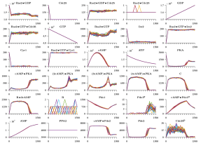
Figure 2: Twenty five draws from the solution to (cme) for the reactions given by Table I–II sampled 15 times uniformly over [0,1500].

Fig. 5 displays the trade-off function for the cases of 3–25 samples. The performance of a random classifier over this data yields an auroc of approximately 0.2. For the cases of 3–6 samples, we note that lasso performs on par with the random classifier. The performance in case of 7–15 samples is better than average with at least 95% certainty (pointwise for each number of samples). Note that there is a trend of increasing performance with increasing samples. Cases of comparatively good or poor performance, like that of 7 and 14 samples respectively can partly be explained by variation in the data. Although not displayed in Fig. 4, more than 25 samples give diminishing returns with respect to the auroc. By identifying the true trade-off function with the sample medians, we could imagine that the shape of the trade-off function is approximately captured by a continuous sigmoid curve.

Consider the inclusion or exclusion of a phosphoproteomic study, i.e., whether the species pde1p, camp • pde1p, and cdc25p are measured or not. Fig. 5 is based on in silico experiments that include phosphoproteomics. The regression parameters $\bm{\mathrm{B}}$ of the best performing model with an aupr of $0.41$ is displayed in Fig. 5. Note that neither pde1p could not be explained using the other data (last row have no true positives), nor is it helpful in explaining the other variables (last column is zero). The protein pde1p contributes a true positive (camp • pde1p in its column) but it is mostly white noise followed by a short and noisy evolution. While the trajectory of pde1p is discernable in Fig. 2, care must be taken as it becomes less so when the number of samples are reduced. However, camp • pde1p is well explained with all positives identified on its row, and also manages to explain the evolution of amp, with two out of four true positives in its column. To have a true positive on the diagonal may not seem impressive, but it is valuable since it indicates that the model makes sense, i.e., that it has some explanatory power aside from mere data fitting.

About 80% of microarray time series in 2006 were short with lengths of 3–8 time points [49]. For a study of the ras/camp/pka pathway in S. cerevisiae where grn inference is done using the lasso method, such time-series would not suffice to infer the topology of the underlying network. It may still be possible to predict how the organism would react to changes in its environment, such as the difference between normal and low glucose levels as represented by the trajectories in Fig. 2 and Fig. 5 respectively. However, that model would not give us clues about the regulatory interactions inside the cell. In theory, it would be possible for an experimentalist that desires such an understanding to consult Fig. 5 and read off the minimum number of samples required to achieve a certain value of the aupr. In practice, the generality of our results need to be increased before it can become a useful tool in the laboratory.

V Discussion

This paper studies the trade-off between quality of inferred gene regulatory network models versus the temporal resolution of data in the case of full and partial state measurements corresponding to an experiment setup that either includes or excludes phosphoproteomics. The goodness of fit is characterized using the area under the curve of the precision-recall curve (aupr). In theory, experimentalists who desires a particular aupr value may consult our graph of the trade-off function to see how many samples are needed to achieve that quality of inference. They can also determine if an increase in the number of samples, or the inclusion of phosphoproteomics, is worthwhile compared to their additional marginal and fixed experimental costs respectively. In practice, it is however clear that additional studies are needed before such a tool becomes mature enough to be of actual use in the laboratory. This paper should be considered as a proof-of-concept study. As such, its purpose is to establish a framework, showcasing how a study of the aforementioned trade-off can be conducted from simulation of data to the evaluation of an inference algorithm.

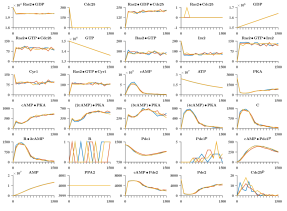
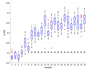
Figure 3: Three draws from the solution to (cme) for the reactions given by Table I–II, except the initial value of gtp is set to $\smash{1.5\cdot 10^{6}}$, sampled 15 times uniformly over [0,1500].

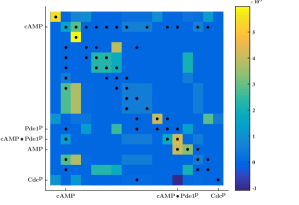
Figure 4: The trade-off function, i.e., the aupr vs. the number of samples, based on 40 in silico experiments. Each sample is represented by a boxplot: the waist is the median, the bottom and top edges of the box indicate the 25th and 75th percentiles respectively. The notches give a 95% confidence interval for the true median. The whisker extend to the extreme data points besides outliers which are represented by plus signs (the whiskers enclose approximately 99.3% of the data if it is normally distributed). The dots denote the performance of a random classifier, $\textsc{aupr}=|\mathcal{F}|/|\mathcal{V}|^{2}$.

Figure 5: Heat map of $\bm{\mathrm{B}}$ with the ground truth as black dots.

References

- [1] Z. Bar-Joseph, A. Gitter, and I. Simon. Studying and modelling dynamic biological processes using time-series gene expression data. Nature Reviews Genetics, 13(8):552–564, 2012.
- [2] H. Kitano. Systems biology: a brief overview. Science, 295(5560):1662–1664, 2002.
- [3] A.-L. Barabasi and Z.N. Oltvai. Network biology: understanding the cell’s functional organization. Nature reviews genetics, 5(2):101–113, 2004.
- [4] Z. Bar-Joseph. Analyzing time series gene expression data. Bioinformatics, 20(16):2493–2503, 2004.
- [5] M.R. Macleod, S. Michie, I. Roberts, U. Dirnagl, I. Chalmers, J.P.A. Ioannidis, R.A.-S. Salman, A.-W. Chan, and P. Glasziou. Biomedical research: increasing value, reducing waste. The Lancet, 383(9912):101–104, 2014.
- [6] A.V. Werhli, M. Grzegorczyk, and D. Husmeier. Comparative evaluation of reverse engineering gene regulatory networks with relevance networks, graphical gaussian models and bayesian networks. Bioinformatics, 22(20):2523–2531, 2006.
- [7] D. Marbach, R.J. Prill, T. Schaffter, C. Mattiussi, D. Floreano, and G. Stolovitzky. Revealing strengths and weaknesses of methods for gene network inference. Proceedings of the national academy of sciences, 107(14):6286–6291, 2010.
- [8] D. Marbach, J.C. Costello, R. Küffner, N.M. Vega, R.J. Prill, D.M. Camacho, K.R. Allison, M. Kellis, J.J. Collins, G. Stolovitzky, et al. Wisdom of crowds for robust gene network inference. Nature methods, 9(8):796–804, 2012.
- [9] A. Aderhold, D. Husmeier, and M. Grzegorczyk. Statistical inference of regulatory networks for circadian regulation. Statistical applications in genetics and molecular biology, 13(3):227–273, 2014.
- [10] C. Sima, J. Hua, and S. Jung. Inference of gene regulatory networks using time-series data: a survey. Current genomics, 10(6):416–429, 2009.
- [11] E. Sefer, M. Kleyman, and Z. Bar-Joseph. Tradeoffs between dense and replicate sampling strategies for high-throughput time series experiments. Cell systems, 3(1):35–42, 2016.
- [12] L. Mombaerts, A. Mauroy, and J. Goncalves. Optimising time-series experimental design for modelling of circadian rhythms: the value of transient data. In Proceedings of the 6th IFAC Conference on Foundations of Systems Biology in Engineering, pages 1–5, 2016.
- [13] D. Husmeier. Sensitivity and specificity of inferring genetic regulatory interactions from microarray experiments with dynamic bayesian networks. Bioinformatics, 19(17):2271–2282, 2003.
- [14] N.D.L. Owens, I.L. Blitz, M.A. Lane, I. Patrushev, J.D. Overton, M.J. Gilchrist, K.W.Y. Cho, and M.K. Khokha. Measuring absolute RNA copy numbers at high temporal resolution reveals transcriptome kinetics in development. Cell reports, 14(3):632–647, 2016.
- [15] S.L. Brunton, J.L. Proctor, and J.N. Kutz. Discovering governing equations from data by sparse identification of nonlinear dynamical systems. Proceedings of the National Academy of Sciences, 113(15):3932–3937, 2016.
- [16] R. Milo, S. Shen-Orr, S. Itzkovitz, N. Kashtan, D. Chklovskii, and U. Alon. Network motifs: simple building blocks of complex networks. Science, 298(5594):824–827, 2002.
- [17] R. Milo, S. Itzkovitz, N. Kashtan, R. Levitt, S. Shen-Orr, I. Ayzenshtat, M. Sheffer, and U. Alon. Superfamilies of evolved and designed networks. Science, 303(5663):1538–1542, 2004.
- [18] J.J. Tyson, K.C. Chen, and B. Novak. Sniffers, buzzers, toggles and blinkers: dynamics of regulatory and signaling pathways in the cell. Current opinion in cell biology, 15(2):221–231, 2003.
- [19] D.J. Wilkinson. Stochastic modelling for quantitative description of heterogeneous biological systems. Nature Reviews Genetics, 10(2):122–133, 2009.
- [20] G. Karlebach and R. Shamir. Modelling and analysis of gene regulatory networks. Nature Reviews Molecular Cell Biology, 9(10):770–780, 2008.
- [21] R. De Smet and K. Marchal. Advantages and limitations of current network inference methods. Nature Reviews Microbiology, 8(10):717–729, 2010.
- [22] H.H. McAdams and A. Arkin. It’s a noisy business! Genetic regulation at the nanomolar scale. Trends in genetics, 15(2):65–69, 1999.
- [23] P. Cazzaniga, D. Pescini, D. Besozzi, G. Mauri, S. Colombo, and E. Martegani. Modeling and stochastic simulation of the ras/camp/pka pathway in the yeast saccharomyces cerevisiae evidences a key regulatory function for intracellular guanine nucleotides pools. Journal of biotechnology, 133(3):377–385, 2008.
- [24] J.A. Tropp and S.J. Wright. Computational methods for sparse solution of linear inverse problems. Proceedings of the IEEE, 98(6):948–958, 2010.
- [25] T. Saito and M. Rehmsmeier. The precision-recall plot is more informative than the ROC plot when evaluating binary classifiers on imbalanced datasets. PloS one, 10(3):e0118432, 2015.
- [26] M.R. Larsen and P.J. Robinson. Phosphoproteomics. In J. Whitelegge, editor, Protein Mass Spectrometry, chapter 12, pages 275–296. Elsevier Science, 2008.
- [27] P.A. Iglesias and B.P. Ingalls. Control theory and systems biology. MIT Press, 2010.
- [28] D.T. Gillespie. A general method for numerically simulating the stochastic time evolution of coupled chemical reactions. Journal of Computational Physics, 22(4):403–434, 1976.
- [29] D.T. Gillespie. Approximate accelerated stochastic simulation of chemically reacting systems. The Journal of Chemical Physics, 115(4):1716–1733, 2001.
- [30] Y. Cao and L.R. Gillespie, D.T.and Petzold. Efficient step size selection for the tau-leaping simulation method. The Journal of chemical physics, 124(4):044109, 2006.
- [31] D.T. Gillespie. Exact stochastic simulation of coupled chemical reactions. The Journal of Physical Chemistry, 81(25):2340–2361, 1977.
- [32] M.A. Gibson and J. Bruck. Efficient exact stochastic simulation of chemical systems with many species and many channels. The journal of physical chemistry A, 104(9):1876–1889, 2000.
- [33] Y. Cao, H. Li, and L. Petzold. Efficient formulation of the stochastic simulation algorithm for chemically reacting systems. The journal of chemical physics, 121(9):4059–4067, 2004.
- [34] D. Besozzi, P. Cazzaniga, D. Pescini, G. Mauri, S. Colombo, and E. Martegani. The role of feedback control mechanisms on the establishment of oscillatory regimes in the ras/camp/pka pathway in s. cerevisiae. EURASIP Journal on Bioinformatics and Systems Biology, 2012(1):10, 2012.
- [35] T. Williamson, J.-M. Schwartz, D.B. Kell, and L. Stateva. Deterministic mathematical models of the camp pathway in saccharomyces cerevisiae. BMC systems biology, 3(1):70, 2009.
- [36] F. Rolland, J. H De Winde, K. Lemaire, E. Boles, J.M. Thevelein, and J. Winderickx. Glucose-induced camp signalling in yeast requires both a g-protein coupled receptor system for extracellular glucose detection and a separable hexose kinase-dependent sensing process. Molecular microbiology, 38(2):348–358, 2000.
- [37] B. Alberts, A. Johnson, J. Lewis, M. Raff, K. Roberts, and P. Walter. Molecular Biology of the Cell. Garland Science, 2008.
- [38] Uri Alon. An introduction to systems biology: design principles of biological circuits. CRC Press, 2006.
- [39] B. Futcher. Cell cycle synchronization. Methods in cell science, 21(2-3):79–86, 1999.
- [40] B.K. Natarajan. Sparse approximate solutions to linear systems. SIAM journal on computing, 24(2):227–234, 1995.
- [41] E. Amaldi and V. Kann. On the approximability of minimizing nonzero variables or unsatisfied relations in linear systems. Theoretical Computer Science, 209(1-2):237–260, 1998.
- [42] E.J. Candès and M.B. Wakin. An introduction to compressive sampling. IEEE signal processing magazine, 25(2):21–30, 2008.
- [43] S. Wright and J. Nocedal. Numerical optimization. Springer Science, 35:67–68, 1999.
- [44] J. Gonçalves and S. Warnick. Necessary and sufficient conditions for dynamical structure reconstruction of lti networks. IEEE Transactions on Automatic Control, 53(7):1670–1674, 2008.
- [45] P. Illari and F. Russo. Causality: Philosophical theory meets scientific practice. Oxford University Press, 2014.
- [46] S. Abbott. Understanding analysis. Springer, 2001.
- [47] T. Fawcett. An introduction to ROC analysis. Pattern recognition letters, 27(8):861–874, 2006.
- [48] D. Mossman. Three-way ROCs. Medical Decision Making, 19(1):78–89, 1999.
- [49] J. Ernst and Z. Bar-Joseph. Stem: a tool for the analysis of short time series gene expression data. BMC bioinformatics, 7(1):191, 2006.