Stellar Population Synthesis of star forming clumps in galaxy pairs and non-interacting spiral galaxies

Abstract

We have identified $1027$ star forming complexes in a sample of 46 galaxies from the Spirals, Bridges, and Tails (SB&T) sample of interacting galaxies, and 693 star forming complexes in a sample of 38 non-interacting spiral (NIS) galaxies in $8\rm{\mu m}$ observations from the Spitzer Infrared Array Camera. We have used archival multi-wavelength UV-to IR observations to fit the observed spectral energy distribution of our clumps with the Code Investigating GALaxy Emission using a double exponentially declined star formation history. We derive the star formation rates (SFRs), stellar masses, ages and fractions of the most recent burst, dust attenuation, and fractional emission due to an active galactic nucleus for these clumps. The resolved star formation main sequence holds on 2.5kpc scales, although it does not hold on 1kpc scales. We analyzed the relation between SFR, stellar mass, and age of the recent burst in the SB&T and NIS samples, and we found that the SFR per stellar mass is higher in the SB&T galaxies, and the clumps are younger in the galaxy pairs. We analyzed the SFR radial profile and found that SFR is enhanced through the disk and in the tidal features relative to normal spirals.

1 Introduction

Galaxy mergers are key ingredients of galaxy mass growth and morphological transformation in the hierarchical scenario of galaxy formation within the standard cosmological model (Springel et al., 2005; Robertson et al., 2006; Bournaud, 2011). Moreover, they were more common at higher redshifts, therefore local galaxy mergers are often used as nearby analogs to improve our understanding of the phenomena involved in high redshift galaxy evolution.

Since Larson & Tinsley (1978) showed evidence of a burst mode of star formation in peculiar galaxies, several studies have found that galaxy interactions can enhance star formation rates by a factor of 2-3 on average relative to their stellar mass (Bushouse, 1987; Kennicutt et al., 1987; Smith et al., 2007; Lin et al., 2007; Li et al., 2008; Knapen et al., 2015). In fact, the most intense star forming galaxies in the nearby Universe, the Ultra Luminous Infrared Galaxies, are mostly driven by mergers (Kim & Sanders, 1998). One might expect that the most intense star forming galaxies at the peak of the cosmic star formation rate, $z\sim 2$ (Madau & Dickinson, 2014) would be driven by mergers. However, even using the same data different authors reach different conclusions (Wisnioski et al., 2015; Rodrigues et al., 2017) due to differences in the merger classification criteria.

Resolved star formation studies of nearby interacting galaxies are crucial to identify which processes are enhancing the star formation. Simulations show that galaxy mergers can produce a loss of axisymmetry, producing gas flows toward the central parts of the galaxies (Mihos & Hernquist, 1996), and therefore central starbursts (Di Matteo et al., 2007). However, more recent high resolution simulations also produced extended star formation due to shock-induced star formation (Barnes, 2004; Chien & Barnes, 2010), or enhanced compressed modes of turbulence (Bournaud, 2011; Powell et al., 2013; Renaud et al., 2014). Analytical models show that tidal disturbances between galaxies perturb the orbits of interstellar clouds, producing high density orbiting crossing zone zones in the outer disks and tidal tails, presumably triggering star formation (Struck & Smith, 2012). However, smoothed particle hydrodynamical (SPH) simulations of pre-merger interacting pairs run by Moreno et al. (2015) find suppressed star formation at radii greater than 1 kpc, compared to isolated galaxies.

Observationally, off-nuclear enhanced star formation is seen in individual cases (Schweizer, 1978; Barnes, 2004; Wang et al., 2004; Smith et al., 2007; Chien & Barnes, 2010; Smith et al., 2010). Larger samples of interacting galaxies are needed to obtain better statistical information on how mergers affect star formation and therefore galaxy evolution. Smith et al. (2016) presented the analysis of $\sim 700$ star forming regions in a sample of 46 galaxy pairs and compared them with those of regions in a sample of 39 normal spiral galaxies, showing that the SFR is proportionally higher for the star forming regions in galaxy pairs. Zaragoza-Cardiel et al. (2015) found an enhancement in electron density, SFR, and velocity dispersion of $\sim 1000$ Hii regions in galaxy pairs compared to $\sim 1000$ Hii regions in non-interacting spirals, analyzing H$\alpha$ emission, consistent with the picture of higher gas turbulence, and higher massive star formation induced by mergers (Bournaud, 2011). Nevertheless, neither dust attenuation nor stellar population were analyzed in Zaragoza-Cardiel et al. (2015), since their main purpose was the study of the internal kinematics of Hii regions with very high spectral resolution.

Stellar population synthesis can be used to obtain the contribution of the interaction to the star formation in terms of the age of the stellar population, and the star formation rate compared to the stellar mass. A well-defined relationship between the global SFR of star-forming galaxies and their stellar mass, $\rm{M_{*}}$, has been discovered (Brinchmann et al., 2004; Salim et al., 2007); this is known as the star formation main sequence of galaxies. This main sequence evolves with redshift out to $z\sim 6$ (Daddi et al., 2007; Chen et al., 2009), but at a given redshift, the scatter in the SFR for a given stellar mass is consistent at $\sim 0.2\thinspace\rm{dex}$ (Speagle et al., 2014). Recently, Cano-Díaz et al. (2016) found that the star formation main sequence still holds on $\rm{kpc}$ scales in a sample of 306 galaxies from The Calar Alto Legacy Integral Field Area survey (CALIFA; Sánchez et al. (2012)), claiming that the star formation process is mainly a local process rather than a global one. Similar recent studies concluded that the resolved star formation main sequence holds on kiloparsec scales in nearby galaxies (Maragkoudakis et al., 2017; Abdurro’uf, 2017) and at redshift $z\sim 1$ (Wuyts et al., 2013; Magdis et al., 2016). performed spatially resolved population synthesis for nine galaxy pairs, and found younger stellar populations than those seen in isolated galaxies. They concluded that this was due to gas flows caused by the interaction.

In the current study we present a stellar population synthesis analysis of the Smith et al. (2016) regions using UV, optical, and IR observations. We then construct the resolved main sequence for the two samples of galaxies and investigate the SFR per stellar mass, the ages of the stellar component, and the spatial extent of the SFR in galaxy pairs. In section $\S 2$ we briefly present the samples, and the photometry of the star forming complexes that were already presented in Smith et al. (2016). In section $\S 3$ we describe the method used to fit the spectral energy distributions (SEDs) of the clumps to model SED. In section $\S 4$ we present the results of the SED analysis, while in section $\S 5$ we show the analysis of the SFR radial variation. Finally, in $\S 6$ we give a discussion and draw our conclusions.

2 Data & clump photometry

2.1 Data

We have previously presented in Smith et al. (2016) the identification of $\sim 700$ star forming complexes in galaxies from the Spirals, Bridges, and Tails (SB&T) sample (Smith et al., 2007, 2010), and star forming complexes in a control sample of non-interacting spiral (NIS) galaxies obtained from Kennicutt et al. (2003); Gil de Paz et al. (2007). We present both samples in Tabs. 2 and 3. The SB&T sample is composed of pre-merger galaxies pairs chosen from the Arp Atlas (Arp, 1966), with velocities $<10,350\rm{km/s}$ and angular sizes $\gtrsim 3\arcmin$, plus NGC 4567/8 and NGC 2207/IC 2163 that are not in the Arp Atlas. The total S&BT sample has 46 pairs, while there are 38 NIS.

The data we used for this study include the GALEX NUV and FUV, Spitzer IRAC 3.6$\mu\rm{m}$, 4.5$\mu\rm{m}$, 5.8$\mu\rm{m}$, 8.0$\mu\rm{m}$, and Spitzer MIPS 24$\mu\rm{m}$ data used in Smith et al. (2016). For the current study, for the 37 out of 46 galaxy pairs, and the 31 out of 38 spirals with optical Sloan Digitized Sky Survey (SDSS) images we used those data as well. The SDSS ugriz filters have effective wavelengths of 3560 $\rm{\AA}$, 4680 $\rm{\AA}$, 6180 $\rm{\AA}$, 7500 $\rm{\AA}$, and 8870 $\rm{\AA}$ respectively. The SDSS FWHM spatial resolution is typically about $1.3\arcsec$. For all of the galaxies in the sample, we also carried out clump photometry using the J, H, and K_S maps from the 2MASS survey. These bands have effective wavelengths of 1.25 $\mu$m, 1.65 $\mu$m, and 2.17 $\mu$m respectively. These images have a spatial resolution of $\sim 4\arcsec$ (Skrutskie et al., 2006).

To determine total fluxes for the sample galaxies in these filters, we used a set of rectangular boxes that covered the observed extent of the galaxy in the images, but avoided very bright stars. These regions included all of the clumps identified in the tidal features (see below for the identification and classification of the clumps). For each image, the sky was determined using rectangular sky regions off of the galaxies without bright stars or other sources. Total fluxes for the individual galaxies in a pair were determined separately and treated separately in the analysis.

2.2 Identification of clumps

We have identified the clumps in smoothed 8 $\mu\rm{m}$ observations from the Spitzer Infrared Array Camera (Fazio et al., 2004). Although the 24 $\mu\rm{m}$ filter is considered a better tracer of star formation than 8 $\mu\rm{m}$ (e.g., Calzetti et al. (2005, 2007)), Spitzer 24 $\mu\rm{m}$ images suffer from more artifacts, and have lower native spatial resolution than the 8 $\mu\rm{m}$ band. The 8 $\mu\rm{m}$ band is also a better choice than H$\alpha$ to identify star forming regions in our sample, since our H$\alpha$ dataset is incomplete and inhomogeneous, and the H$\alpha$ is strongly affected by dust absorption. The UV bands also suffer from extinction, thus a clump search on UV maps may miss the most obscured regions in interacting galaxies and may produce positions that are offset from the peak of the star formation (Smith et al., 2014).

For the identification of clumps, two different Gaussian smoothings were used, one that produces a FWHM resolution of 1 kpc, and the other of 2.5 kpc. As described in detail in Smith et al. (2016), clumps were selected automatically from the smoothed images using the Image Reduction and Analysis Facility (IRAF) daofind routine (Stetson, 1987) using a detection threshold of 10 sigma above the noise level. The daofind parameters sharplo, sharphi, roundlo, and roundhi were set to 0.1, 1.2, -2.0, and 2.0, respectively, to allow slightly extended and/or elongated clumps. The images were then inspected visually, to eliminate spurious detections due to artifacts in the images. We show in Fig. 1 the identified clumps: (a) 1kpc, (b) 2.5kpc; for Arp 82 in all the observed bands.

Figure 1: GALEX, SDSS, H$\alpha$, 2MASS, and Spitzer images of Arp 82. (a) Identified clumps at 1kpc scales. (b) Identified clumps at 2.5 scales. Black circles are clumps in the disk, white are those in the tails, and gray are those in the nucleus.

2.3 Photometry of the clumps

The photometry of the clumps was then performed on the unsmoothed images using the IRAF daophot routine with aperture radii of 1.0 and 2.5 kpc, respectively. The local galaxian background was calculated using a sky annulus with an inner radius equal to the aperture radius, and an annulus width equal to 1.2 $\times$ the aperture radius. The mode sky fitting algorithm was used to calculate the background level, as the mode is considered most reliable in crowded fields (Stetson, 1987). The poorer spatial resolution in the GALEX bands and at 24 $\mu\rm{m}$ may lead to greater clump contribution to the sky background, and so slightly lower fluxes.

The fluxes were then aperture-corrected to account for spillage outside of the aperture due to the image resolution. For the GALEX, 2MASS, and SDSS images, the aperture corrections were calculated for each image individually. For each image, aperture photometry for three to ten moderately bright isolated point sources was done using our target aperture radius, and then comparing with photometry done within a $17\arcsec$ radius. More details on this process are provided in Smith et al. (2016). For the Spitzer data, rather than calculating aperture corrections ourselves we interpolated between the tabulated values of aperture corrections provided in the IRAC and MIPS Instrument Handbooks . We were not able to calculate aperture corrections for the H$\alpha$ fluxes because of the lack of isolated off-galaxy point sources on the H$\alpha$ maps. The aperture corrections for H$\alpha$ are expected to be small because of the relatively high spatial resolution ($0.7\arcsec$ to $1.5\arcsec$). If the intrinsic size of a clump is large compared to our aperture radii, our aperture corrections (which assume point sources) may underestimate the true fluxes, particularly for bands with poor intrinsic resolution. For example, some of the clumps may be blends of multiple smaller clumps, with one of our clumps consisting of several smaller components. Alternatively, a clump may be a single physically-large object. In these cases, our final fluxes in the filters with lowest resolution (GALEX and Spitzer 24 $\mu\rm{m}$), may be somewhat under-estimated compared to filters with better spatial resolution.

We used the $1\rm{kpc}$ radii clumps to study star formation on smaller scales for the 30 galaxy pairs and 36 NIS galaxies closer than $67\thinspace\rm{Mpc}$, and used the $2.5\rm{kpc}$ radii clumps to study star formation on a larger scale in the whole sample; $2.5\rm{kpc}$ is the limiting resolution ($6\arcsec$ FWHM in GALEX and Spitzer $24\rm{\mu m}$). This choice of parameters allowed us to obtain accurate photometry even in the furthest galaxy, Arp107 at $142\rm{Mpc}$.

In Table 4 we present the photometry for GALEX: NUV and FUV; IRAC: $3.6\rm{\mu m}$, $4.5\rm{\mu m}$, $5.8\rm{\mu m}$, $8.0\rm{\mu m}$; MIPS $24\rm{\mu m}$; SDSS: u, g, r, i, z; H$\alpha$+cont, continuum subtracted H$\alpha$, and 2MASS: J, H, K. Three different classifications for the clumps in the SB&T sample were used as explained in Smith et al. (2016): clumps in the disk, in tails, and in the nuclear region; for the clumps in the NIS sample we classified the clumps in the disk, and those in nuclear regions. Thus, the column containing the name of the clumps consists of the name of the system (galaxy in the case of NIS galaxies), consecutive identification number, the sample to which it belongs, location, and radius of the aperture in kiloparsec. In the fourth column of Table 4, we provide the galaxy name; for the SB&T galaxies, this is the name of the individual galaxy in the pair the clump is associated with.

3 SED modeling

Table 1: CIGALE parameters

Free parameters
$e$-folding time of the old population	2, 4, 6 Gyr
$e$-folding time of the late starburst population	5, 10, 25, 50, 100 Myr
Mass fraction of the late burst population	0, 0.2, 0.4, 0.6, 0.8, 0.99
Age of the late burst	1, 5, 10, 15, 20, 25, 30, 40, 50, 60, 70, 80,
	90, 100, 150, 200, 250, 300, 400, 500 Myr
Metallicity	0.008, 0.02, 0.05
E(B$-$V) of the stellar continuum light for the young population.	0.01, 0.2, 0.4, 0.6, 0.7 mag
Amplitude of the UV bump	0, 1, 2, 3
Slope $\delta$ of the power law modifying the attenuation curve	-0.5, -0.3, -0.1, 0.0
AGN fraction (just for nuclear regions)	0.0,0.2,0.4,0.6,0.8,0.99
$\alpha$ slope	1.0, 1.5, 2., 2.5, 3., 3.5, 4.
Fixed parameters
Age of the oldest stars	13 Gyr
Reduction factor for the E(B-V) of the old population compared to the young one	0.44
IMF	Chabrier (2003)
Ionization parameter	$10^{-2}$
Fraction of Lyman continuum photons absorbed by dust	10%
Fraction of Lyman continuum photons escaping the galaxy	0%

We use the Code for Investigating GALaxy Emission (CIGALE, Noll et al. (2009)), python version 0.9, to model and fit the SEDs for each individual clump.

CIGALE is based on the assumption of an energy balance between the energy absorbed in the UV, optical, and NIR, and re-emitted by the dust in the MIR and FIR. CIGALE uses the dust emission model of Dale et al. (2014) which is dependent on the relative contribution of different heating intensities, $U$, modeled by the exponent $\alpha$ in the spatially integrated dust emission $dM_{d}\propto U^{\alpha}dU$, where $M_{d}$ is the dust mass heated by a radiation intensity $U$ (Dale & Helou, 2002). We leave $\alpha$ as a free parameter, and for the nuclear regions we also leave the AGN fraction contribution as a variable (see Table 1) while for the rest of the clumps we set the AGN fraction contribution to zero. To model dust attenuation, CIGALE assumes a combination of dust attenuation curves from Calzetti et al. (2000) and Leitherer et al. (2002) and modifies them by a power law centered at $550\rm{nm}$, with exponent $\delta$ (free parameter), and adds a UV bump with a specific amplitude (free parameter). We fix the differential reddening, and leave the color excess E(B-V) as a free parameter.

In order to model the plausible recent star formation enhancement in galaxy pairs, we model the star formation history with two decaying exponentials:

$${\rm{SFR}}(t)=(1-f_{\rm{y}})\thinspace{\rm{SFR_{0\thinspace old}}}\thinspace e^{-\frac{t-t_{1}}{\tau_{1}}}+f_{\rm{y}}\thinspace{\rm{SFR_{0\thinspace young}}}\thinspace e^{-\frac{t-t_{2}}{\tau_{2}}}$$ (1)

as described in Serra et al. (2011), where the $e$-folding times ($\tau_{i}$), the mass fraction of the recent starburst ($f_{\rm{y}}$), and the age ($t_{2}$) of the recent starburst, are left as free parameters, while the age of the oldest stars ($t_{1}$) is set (see Table 1 for values). We use the stellar populations of Bruzual & Charlot (2003) considering the Chabrier (2003) initial mass function, and three possible values of metallicity (around solar). The CIGALE parameters are summarized in Table 1.

The aforementioned set of parameters yields $3\cdot 10^{6}$ models for non-nuclear regions and $1.8\cdot 10^{7}$ models for nuclear regions, and then CIGALE performs a Bayesian analysis for each output parameter as described in Noll et al. (2009), resulting in the estimated values and uncertainties given in Table 5. To be sure of the goodness of the fit, we include only the clumps for which the fit of the SED yields $\chi^{2}_{\rm{red}}<10$. For those clumps with no SDSS observations ($27\%$) the relative uncertainties of the resulting parameters are on average only $2\%$ larger, thus we can include them in the analysis directly with the rest of the clumps. Additionally, since we are interested in the study of recent star formation, we do not consider in the following analysis the clumps and galaxies with no present star formation, i. e. , $f_{\rm{y}}=0$.

3.1 SED vs. photometric star formation rates

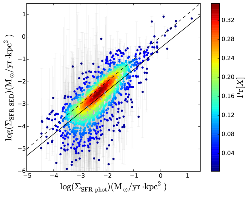
Figure 2: Instantaneous SFR surface density derived from the SED fitting, $\Sigma_{\rm{SFR\,SED}}$, versus the SFR surface density presented in Smith et al. (2016), $\Sigma_{\rm{SFR\,phot}}$, color coded with the probability distribution function derived from the data points, ${\rm{Pr}}[X]$. The solid line represents the variable $x$-bin size linear fit (Eq. 2), while the dashed line represents the one to one relation.

We plot in Fig. 2 the instantaneous SFR surface density derived from the SED fitting, $\Sigma_{\rm{SFR\,SED}}$, versus the photometric SFR surface density derived from UV + IR fluxes, $\Sigma_{\rm{SFR\,phot}}$, presented in Smith et al. (2016), for all the identified clumps. These points are color coded with the probability distribution function (PDF) derived from the data points, ${\rm{Pr}}[X]$. We use the same color code in the later figures of this work where we color coded with the PDF. The variable $x$-bin size linear fit (solid line) yields:

$$\log(\Sigma_{\rm{SFR\,SED}})=(0.96\pm 0.03)\cdot\log(\Sigma_{\rm{SFR\,phot}})-(0.49\pm 0.08).$$ (2)

Thus, using the SFR obtained from the SED fitting is equivalent to using the photometric SFR presented in Smith et al. (2016), since they just differ in a constant shift compared to the one to one relation (dashed line in Fig. 2). We will use in the following analysis the instantaneous SFR derived from the SED fitting.

4 Results

4.1 Integrated star formation main sequence

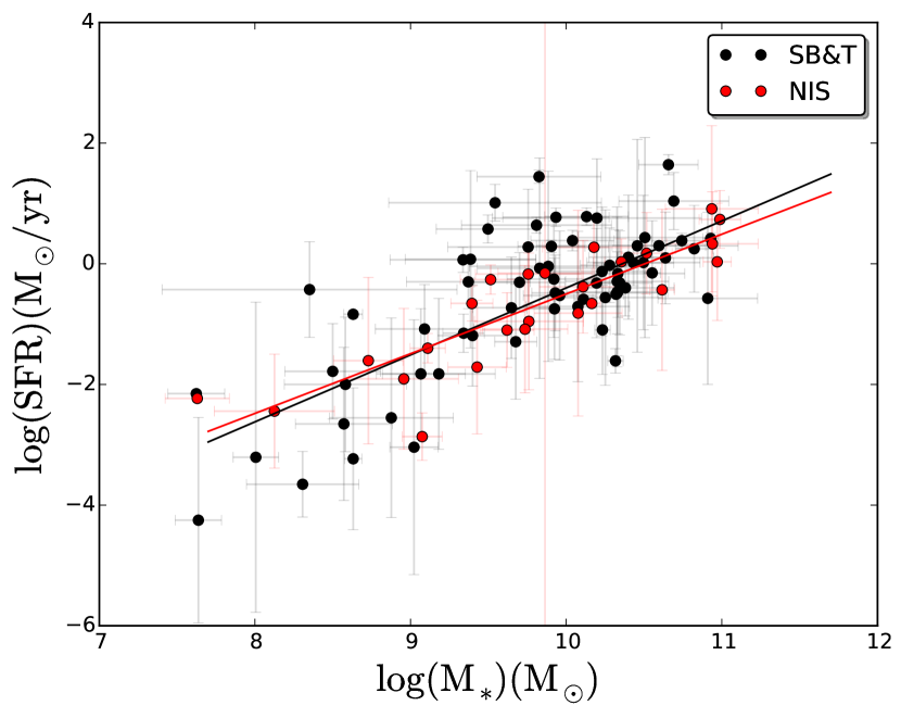
Figure 3: Star formation rate, $\rm{SFR}$, versus stellar mass, $\rm{M_{*}}$, for the SB&T galaxies (black) and NIS galaxies (red). The lines are the linear fits to the data points.

We obtained integrated aperture photometry for each galaxy in the SB&T and NIS sample in the same bands as in the clumps. The integrated photometry is presented in Tab. 6. Then, we used the same set of CIGALE parameters (Table 1) to derive the integrated SFR and $M_{*}$ for each galaxy. We plot the star formation main sequence, SFR versus $M_{*}$, in Fig. 3 for the SB&T galaxies in black, and the NIS in red. We perform linear fits to both samples separately, and we obtain:

$$\log(\rm{SFR})\left(\frac{\rm{M_{\odot}}}{\rm{yr}}\right)=(1.11\pm 0.13)\log(\rm{M_{*}})\left(\rm{M_{\odot}}\right)-(11.5\pm 1.2),$$ (3)

for SB&T galaxies (black line in Fig 3), and

$$\log(\rm{SFR})\left(\frac{\rm{M_{\odot}}}{\rm{yr}}\right)=(0.99\pm 0.12)\log(\rm{M_{*}})\left(\rm{M_{\odot}}\right)-(10.4\pm 1.2),$$ (4)

for NIS (red line in Fig 3). The scatter of the integrated star formation main sequence after removing the average uncertainty by quadrature is 0.47 dex for SB&T galaxies and 0.28 dex for NIS galaxies.

The slopes are in agreement, therefore both samples are in the main sequence of star formation, although the SB&T sample presents more scatter in that relation. The slopes (Eqs. 3 and 4) are in the range of observed values 0.6-1 (Rodighiero et al., 2011).

4.2 Resolved star formation main sequence

The results are based on 879 clumps from the SB&T galaxies, and 541 clumps from the NIS galaxies.

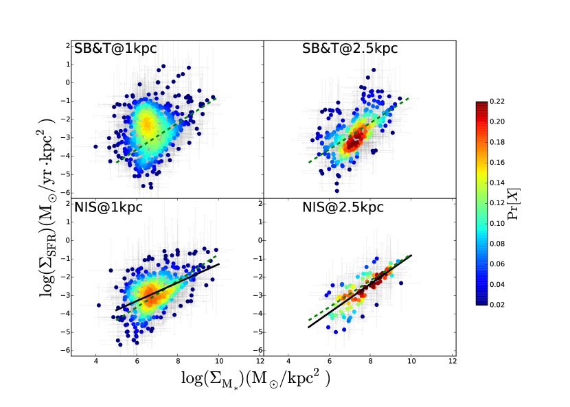
Figure 4: Resolved star formation rate per area, $\Sigma_{\rm{SFR}}$, versus resolved stellar mass per area, $\Sigma_{\rm{M_{*}}}$, for clumps identified in the SB&T galaxies (top) and NIS galaxies (bottom). The solid black lines are the linear fits with variable $x-bin$ size. The dashed green line is the resolved star formation main sequence from Cano-Díaz et al. (2016).

In Smith et al. (2016) we already showed that the clumps in the SB&T galaxies have higher SFRs compared to those in NIS. Here, we explore the differences in the SFR between SB&T and NIS galaxies relative to the stellar mass of the clumps.

We show in Fig. 4 the resolved SFR per area, $\Sigma_{\rm{SFR}}$, versus the resolved stellar mass per area, $\Sigma_{\rm{M_{*}}}$. Cano-Díaz et al. (2016); Maragkoudakis et al. (2017); Abdurro’uf (2017) have already shown that the resolved star formation main sequence holds on kiloparsec scales in nearby galaxies. Here, we show that for the clumps in the SB&T galaxies, the resolved star formation main sequence presents a different pattern compared to the clumps in the control sample of NIS on 1kpc scales. More precisely, there is no linear correlation between SFR and stellar mass, with a large fraction of clumps displaying excess SFR at $\log(\Sigma_{\rm{M_{*}}})(\rm{M_{\odot}/kpc^{2}})\sim 6.5$. Although a comparable cloud of points is seen in the clumps of the NIS galaxies sample on 1kpc scales, it is seen to be weaker than that in the SB&T sample. It is notable that when the results are considered on 2.5kpc scales, the cloud of points with an SFR excess vanishes in the SB&T galaxies and also in the NIS. Thus, the resolved star formation main sequence does not hold on kiloparsec scales.

In order to quantify deviations and enhancements compared with the star formation main sequence, we perform a variable $x-bin$ size fit to the $\Sigma_{\rm{SFR}}$-$\Sigma_{\rm{M_{*}}}$ data points for NIS on 1 and 2.5kpc scales. The variable $x-bin$ size fit allow us to weight by the density of data points, assuming a constant number of data points in each bin. We know that the resolved star formation main sequence for NIS on 1 kpc scales deviates from a linear relation (Fig. 4 bottom-left). Thus, the linear fit in this case is an approximation to measure the deviation of the SB&T clumps from the NIS clumps on 1 kpc scales. The results of the linear fits for the NIS galaxies are:

$$\begin{array}[]{ll}\log(\Sigma_{\rm{SFR}})\left(\frac{\rm{M_{\odot}}}{\rm{yr\thinspace kpc^{2}}}\right)=\\ (0.50\pm 0.06)\log(\Sigma_{\rm{M_{*}}})\left(\frac{\rm{M_{\odot}}}{\rm{kpc^{2}}}\right)-(6.3\pm 0.4),\end{array}$$ (5)

for $1\thinspace\rm{kpc}$ scales, and

$$\begin{array}[]{ll}\log(\Sigma_{\rm{SFR}})\left(\frac{\rm{M_{\odot}}}{\rm{yr\thinspace kpc^{2}}}\right)=\\ (0.78\pm 0.05)\log(\Sigma_{\rm{M_{*}}})\left(\frac{\rm{M_{\odot}}}{\rm{kpc^{2}}}\right)-(8.6\pm 0.4),\end{array}$$ (6)

for $2.5\thinspace\rm{kpc}$ scales. The scatter of the resolved main sequence of star formation in NIS after removing the mean uncertainty of the estimated SFR by quadrature is $0.41\thinspace\rm{dex}$ for $1\thinspace\rm{kpc}$ scales, and $0.36\thinspace\rm{dex}$ for $2.5\thinspace\rm{kpc}$ scales, both of these values are larger than those found by Cano-Díaz et al. (2016), although similar to those found by Maragkoudakis et al. (2017); Abdurro’uf (2017), and larger compared to the scatter of the integrated main sequence of star formation for NIS galaxies. These results, shown as a solid black line in Fig. 4 (bottom), show that the resolved star formation main sequence for the two sets of galaxies is different on 1kpc scales. The slope for the NIS is lower on 1kpc scales due to the excess of SFR at $\log(\Sigma_{\rm{M_{*}}})(\rm{M_{\odot}/kpc^{2}})\sim 6.5$, which is also present in the SB&T clumps on those scales.

Figure 5: Histograms of the SFR excess of the clumps in the SB&T galaxies (solid black line), and in NIS galaxies (solid red line), normalized to the total number of clumps in the SB&T galaxies and NIS, respectively. The histograms of the SFR excess of the clumps in tails (black dotted line), in disks (dashed black line), and in the nuclei (blue solid line) of the SB&T galaxies, are normalized to the total number of clumps in the SB&T galaxies. The histogram of SFR excess of the clumps in disks (green dashed line) and in the nucleus (green solid line) of the NIS galaxies, is normalized to the total number of clumps in NIS galaxies. Top: Clumps on $1\rm{kpc}$ scales. Bottom: Clumps on $2.5\rm{kpc}$ scales. The SFR excess is defined as the difference between the SFR derived from the SED modeling and the one derived from Eqs. 5 and 6.

We define the $\rm{SFR_{excess}}$ as the difference between the SFR surface density obtained by the SED modeling and the SFR obtained using Eqs. 5 and 6, and using the stellar mass from Tab. 5. The $\rm{SFR_{excess}}$ represents the deviation of the observed SFR from that expected, as derived from the resolved main sequence of star formation determined for NIS galaxies. We show in Fig. 5 the histograms of the $\rm{SFR_{excess}}$ normalized to the total number of clumps in the SB&T galaxies (solid black line), and the number of clumps in NIS (solid red line). We also show the histograms of the SFR excess for the clumps in tails (black dotted line), in the disks (dashed black line), and in the nucleus (blue solid line), of the SB&T galaxies, normalized to the total number of clumps in the SB&T galaxies. We observe that there is a population of clumps with higher SFR excess in the SB&T galaxies, present in the tail, disk, and nuclear clumps, compared to the clumps in NIS on both $1\rm{kpc}$ scales (top), and $2.5\rm{kpc}$ scales (bottom). SFR excesses in the clumps in the SB&T galaxies are probably induced by the interaction, and make a very good case for studying the triggered star formation regime in galaxy pairs. In the higher SFR excess clump population, the star formation is not a local process as claimed by Cano-Díaz et al. (2016), but a global process, because it is affected and enhanced by the interaction.

On 1kpc scales, the resolved star formation main sequence is different compared to that at $2.5\rm{kpc}$ even in NIS galaxies, pointing toward a break of the star formation main sequence on smaller scales. Cano-Díaz et al. (2016); Maragkoudakis et al. (2017); Abdurro’uf (2017) did not observe this break probably because they are based on pixel-to-pixel SED fitting, while in this work we perform the SED fitting based on clumps, i. e. , in maximum peaks of star formation, and we subtracted the local galaxian background for each clump. Thus, finding an excess of SFR with respect to the stellar mass is more plausible with our method.

Figure 6: (a) Specific SFR at 1kpc scales, $\rm{sSFR_{1kpc}}$, versus specific SFR at 2.5kpc scales, $\rm{sSFR_{2.5kpc}}$. (b) SFR at 1kpc scales, $\rm{SFR_{1kpc}}$, versus SFR at 2.5kpc scales, $\rm{SFR_{2.5kpc}}$. (c) Stellar mass at 1kpc scales, $M_{\rm{*\,1kpc}}$, versus stellar mass at 2.5kpc scales, $M_{\rm{*\,2.5kpc}}$. (d) Histograms of the distance between center of clumps at 2.5kpc scales and clumps at 1kpc scales, $\rm{Dist_{2.5kpc\,-\,1kpc}}$. All of the plots are for those clumps at 2.5kpc scales which have 1kpc clumps inside them. Clumps from the SB&T sample are in black, and clumps from the NIS sample are in red. The dashed lines are the 1 to 1 relation.

We have cross-correlated the two sets of clumps (1kpc and 2.5kpc) to find 1kpc clumps within 2.5kpc clumps. In Fig. 6 we show the specific SFR (a), the SFR (b), and the stellar mass (c), at both scales for clumps at 2.5kpc, which have one or more 1kpc clump inside them. The specific SFR at 1kpc scales is larger compared to that of clumps at 2.5kpc scales, which explains the larger SFR excess found at 1kpc scales for both SB&T (black circles) and NIS (red circles) samples. On average, the sSFR is 4 times larger at 1kpc scales compared to 2.5kpc scales. This is due to the fact that the SFR is more centrally concentrated than the older stellar population as can be seen in Figs. 6 (b) and (c), since the SFR at 1kpc vs SFR at 2.5kpc distribution is closer to the one to one relation at both scales, while the stellar mass at 2.5 kpc is larger than the stellar mass at 1kpc scales. In addition, in Fig. 6 (d) we plot the histograms of the distances between the centers of the clumps at 2.5kpc and at 1kpc, $\rm{Dist_{2.5kpc\,-\,1kpc}}$, for those 2.5kpc clumps which have one or more 1kpc inside them. The distances are dominated by a population of clumps at both scales having the same centers, which means that the strongest star formation tends to occurs at the center of large old stellar clumps. However, there is a population of clumps at both scales having very different centers ($\rm{Dist_{2.5kpc\,-\,1kpc}}>1\rm{kpc}$). If we consider that 1 kpc clump is within a 2.5kpc clump if at least half of it is completely inside, just 47 clumps at 2.5kpc have two or more 1kpc clumps within them out of 381 2.5kpc identified clumps. Then, we can neglect the effect of blending.

4.3 Recently induced star formation

Figure 7: SFR excess versus the age of the recent starburst, color coded with the PDF. The figure displays clumps in the SB&T galaxies (top) and in the NIS galaxy sample (bottom). The SFR excess is defined as the difference between the SFR derived from the SED modeling and that derived from Eqs. 5 and 6.

In order to explore the possible connection between the higher SFR excess of clumps in the SB&T galaxies and their recent interaction history, we compared the derived age of the recent burst ($t_{2}$ in Eq. 1) from the SED fitting with the SFR excess. We plot in Fig. 7 the SFR excess versus the age of the recent burst for clumps in the SB&T galaxies (top) and in the NIS galaxies (bottom), color coded with the PDF. Fig. 7 shows that the SFR excess depends on the age of the recent burst of star formation; the younger the recent burst, the higher the SFR excess. Additionally, the density of data points shows that the SB&T galaxies have a population of clumps which have a younger recent burst of star formation, notably at $\log(\rm{Burst\thinspace Age})\sim 1.9$, and also at $\log(\rm{Burst\thinspace Age})<1$, compared to the NIS galaxies. Therefore, the triggering of the SFR excess in the SB&T galaxies is evidently due to a recent event such as the interaction with a companion galaxy.

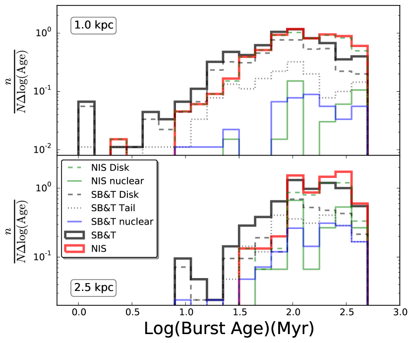
Figure 8: Age of the recent starburst histograms for clumps in the SB&T galaxies (solid black line), and for clumps in the NIS galaxies (solid red line), normalized by the total numbers of clumps in the SB&T galaxies and the total number of clumps in the NIS galaxies, respectively. Top: Clumps at 1kpc scales. Bottom: Clumps at 2.5kpc scales. The black dotted lines are the age of the recent starburst histograms of the clumps in tails, the dashed black lines are the age of the recent starburst histograms of the clumps in the disks, and the solid blue lines are the recent starburst histograms of the clumps in the nucleus for clumps in the SB&T sample, and normalized by the total number of clumps in the SB&T sample. The solid and dashed green lines are the age of the recent starburst histograms of the clumps in the nucleus and in the disks, respectively, for clumps in the NIS galaxies, and normalized by the total number of clumps in the NIS galaxies.

Histograms of the age of the recent burst (Fig. 8) show that there is a population of clumps in the SB&T galaxies (solid black lines) with smaller ages compared to the NIS galaxies (solid red line) on both scales. Younger recent burst ages are found in the tails (black dotted line), the disks (dashed black line), and the nuclei (blue solid line) of the SB&T galaxies. These results show that there are more recent bursts of star formation in the clumps of the SB&T galaxies induced by the interactions, which enhance the observed SFR excess.

5 SFR radial profile

Figure 9: Isophotal radius at $25\thinspace\rm{mag/arcsec^{2}}$ in the B-band, $R_{25}$, versus the effective radius in the J band from 2MASS, $R_{\rm{eff}}$, for SB&T and NIS galaxies. The solid line is the linear fit to the data points, while the dashed line is the 1 to 1 one relation.

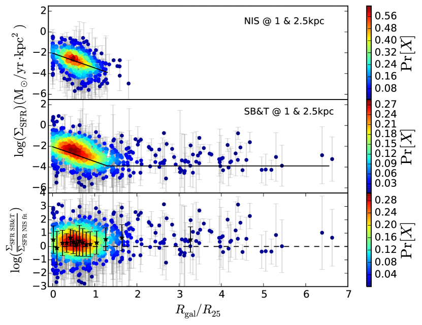
Figure 10: Top: SFR surface density, $\Sigma_{\rm{SFR}}$, versus the galactocentric radius normalized by the isophotal radius at $25\thinspace\rm{mag/arcsec^{2}}$ in the B-band, $R_{\rm{gal}}/R_{25}$, of the clumps in disks from the NIS galaxies, color coded with the PDF. The solid black line is the variable $x$-bin size fit to the points. Middle: SFR surface density, $\Sigma_{\rm{SFR}}$, versus the galactocentric radius normalized by the isophotal radius at $25\thinspace\rm{mag/arcsec^{2}}$ in the B-band, $R_{\rm{gal}}/R_{25}$, of the clumps in disks and tails from the SB&T galaxies sample, color coded with the PDF. The solid black line is the fit to the points of the clumps in NIS galaxies (top panel), and for $R_{\rm{gal}}/R_{25}>1.15$ we extrapolate the value of the fit as a constant one. Bottom: Ratio between the SFR surface density for clumps in the SB&T galaxies and the SFR surface density derived from the linear fit for clumps in NIS (Eq. 7), $\Sigma_{\rm{SFR\thinspace SB\&T}}/\Sigma_{\rm{SFR\thinspace NIS\thinspace fit}}$, versus the galactocentric radius normalized by the isophotal radius at $25\thinspace\rm{mag/arcsec^{2}}$ in the B-band, $R_{\rm{gal}}/R_{25}$, of the clumps in disks and tails from the SB&T galaxies sample, color coded with the PDF. We show the median values of the $\Sigma_{\rm{SFR\thinspace SB\&T}}/\Sigma_{\rm{SFR\thinspace NIS\thinspace fit}}$ for a variable $x$-bin size as a black star symbols, with their standard deviations as error bars.

The SB&T sample of galaxies is composed of galaxy pairs in an early-intermediate stage of the merger process, while advanced mergers are excluded. Therefore, the distortions are small enough to be able to study the SFR radial profile for the clumps in the SB&T sample, in order to see the radial variation of the SFR enhancement.

We normalized the galactocentric radius of each identified clump by the isophotal radius at $25\thinspace\rm{mag/arcsec^{2}}$ in the B-band, in order to compare all the galaxies from both samples together. We obtained the inclinations, position angles, and lengths of the major axis at the isophotal level $25\thinspace\rm{mag/arcsec^{2}}$ in the B-band, from the Hyperleda database (Makarov et al., 2014) for each galaxy (see Tabs. 2 and 3). We show in Fig. 9 the isophotal radius at $25\thinspace\rm{mag/arcsec^{2}}$ in the B-band, $R_{25}$, versus the effective radius in the J band from 2MASS, $R_{\rm{eff}}$, for SB&T and NIS galaxies. We obtained J band $R_{\rm{eff}}$ from the 2MASS All-Sky Extended Source Catalog (Skrutskie et al., 2006). Since the surface brightness is independent of distance, the choice of isophotal or effective radius is just affected by a constant factor, thus the selection of the isophotal radius does not affect the results presented below.

For the SB&T galaxies, we obtained those parameters for each individual galaxy and associate each clump with one of the galaxies to normalize the galactocentric radius of each clump with the corresponding isophotal radius of his galaxy. The Galaxy column in Tab. 4 refers to the specific galaxy from the galaxy pair the clump is associated with.

Several studies show that the spatial distribution of the SFR in spirals approximately follows an exponential profile (Hodge & Kennicutt, 1983; Athanassoula et al., 1993; Ryder & Dopita, 1994; Koopmann et al., 2006). Thus, we plot in Fig. 10 (top) the SFR surface density, $\Sigma_{\rm{SFR}}$, of the clumps in disks from the NIS galaxies, versus the galactocentric radius normalized by the isophotal radius at $25\thinspace\rm{mag/arcsec^{2}}$ in the B-band, $R_{\rm{gal}}/R_{25}$, color coded with the PDF, and we perform a variable $x$-bin size fit to the data, obtaining

$$\log(\Sigma_{\rm{SFR}})=(-1.42\pm 0.10)\thinspace R_{\rm{gal}}/R_{25}-(2.04\pm 0.06).$$ (7)

The variable $x-bin$ size fit allows us to weight by the density of data points, assuming a constant number of data points in each bin.

In the middle panel of Fig. 10 we plot $\Sigma_{\rm{SFR}}$ versus $R_{\rm{gal}}/R_{25}$, of the clumps in the disks and tails of the SB&T galaxies, color coded with the PDF. We add to this plot the fit from the clumps in NIS (top panel) to compare how the SFR radial profile differs in both samples. We extrapolate the last value of Eq. 7 for the last radial bin for the NIS galaxies to larger radii, to compare with the tidal features of the SB&T galaxies.

$\Sigma_{\rm{SFR}}$ is on average larger in SB&T clumps compared to NIS clumps. To study in more detail the differences between the SFR radial profiles in the SB&T and NIS galaxies samples, we derive $\Sigma_{\rm{SFR\thinspace SB\&T}}/\Sigma_{\rm{SFR\thinspace NIS\thinspace fit}}$, which is the ratio between the observed $\Sigma_{\rm{SFR}}$ and that derived from Eq. 7 and the extrapolation using the corresponding $R_{\rm{gal}}/R_{25}$ value for the clumps in disks and tails from the SB&T galaxies. We plot $\Sigma_{\rm{SFR\thinspace SB\&T}}/\Sigma_{\rm{SFR\thinspace NIS\thinspace fit}}$ versus $R_{\rm{gal}}/R_{25}$ in the bottom panel of Fig. 10, where we show how the SFR surface density increases toward the central parts of the SB&T galaxies compared to the NIS between $R_{\rm{gal}}/R_{25}\in[0.4,0.9]$, which is in agreement with theoretical models of galaxy interactions, where gas inflows are produced by the loss of axisymmetry. There is less SFR enhancement toward inner regions $R_{\rm{gal}}/R_{25}<0.4$, except the nuclear regions, which present a median enhancement of 2.4.

In Fig. 10 (bottom) we also show that the SFR surface density increases toward the external parts of the SB&T galaxies compared to the NIS between $R_{\rm{gal}}/R_{25}\in[1,6.5]$. We extrapolate the exponential fit derived (Eq. 7) to external regions using the value of the last radial bin from the NIS galaxies, since we do not observe clumps in the NIS galaxies beyond $R_{\rm{gal}}/R_{25}\sim 2$. Although this extrapolation may not represent the real values, it is a conservative upper limit of $\Sigma_{\rm{SFR}}$ for the clumps in NIS. The SFR enhancement in the external parts of galaxy mergers is highly debated because the evidence of the enhancement has been based on individual cases. Here, we present evidence for a larger sample of galaxy pairs in intermediate-early stages of interaction, where the SFR is clearly enhanced far from the nucleus. We obtain an SFR enhancement for clumps in the SB&T galaxies where $R_{\rm{gal}}/R_{25}>2$ of $\frac{\Sigma_{\rm{SFR\thinspace SB\&T}}}{\Sigma_{\rm{SFR\thinspace NIS\thinspace fit}}}>2.1$.

6 Discussion & Conclusion

We present stellar population synthesis analysis of 879 clumps from the SB&T galaxy sample, and 541 clumps from the NIS galaxy sample using the CIGALE SED modeling code, and UV, optical, and IR photometry of the clumps. Using CIGALE we obtained SFRs, stellar masses, ages of the most recent burst, and fractions of the most recent burst, for the identified clumps.

The resolved star formation main sequence was presented by Cano-Díaz et al. (2016); Maragkoudakis et al. (2017); Abdurro’uf (2017) for nearby galaxies, where they showed that it does hold on kiloparsec scales ($[1-2\rm{kpc}]$). However, we find that for the identified clumps at 1kpc scales, the main sequence begins to breakdown in the NIS galaxies, and more intensely in the SB&T galaxies, while for the clumps at 2.5kpc scales the main sequence holds, although it presents a higher scatter compared to that of the integrated star formation main sequence for NIS galaxies. We selected those scales in an effort to study star formation in higher resolution (1kpc) due to the proximity of the sources to us (those with $D<67\thinspace\rm{Mpc}$), and also to study star formation for all the galaxies. We were limited by the most distant galaxy, Arp 107, at $142\thinspace\rm{Mpc}$, and the resolution of the GALEX and Spitzer 24 $\mu$m images, which approximately corresponds to $2.5\thinspace\rm{kpc}$ at $142\thinspace\rm{Mpc}$. We show that the resolved star formation main sequence breaks down at small scales (between $1\thinspace\rm{kpc}$ and $2.5\thinspace\rm{kpc}$). As in the case of the Kennicutt-Schmidt law, which breaks down for sub-kpc scales (Bigiel et al., 2008; Onodera et al., 2010), a break is expected a small scales since stellar mass and star formation rate trace different properties of the star formation process, and these breaks could be used to constrain unknown quantities related to the star formation such as the duration of different star formation phases (Kruijssen & Longmore, 2014).

The breakdown is more notable in the clumps from the SB&T galaxies, where the SFR is higher per stellar mass compared to the clumps in NIS galaxies. The SFR excess in the SB&T galaxies is probably triggered from the interactions, since they drive gas flows, increase turbulence, and compress gas. Therefore, at least in the nearby universe, the SFR surface density and the stellar mass surface density relation was affected by the environment, where galaxy pairs present higher SFR excess. Mergers should not be important drivers of the SFR enhancement observed at higher redshifts (Madau & Dickinson, 2014), because the star formation main sequence has been observed to be tight even at high redshifts (Rodighiero et al., 2011; Speagle et al., 2014). Thus, higher gas fractions have been proposed as a mechanism to enhance SFR at higher redshift, and when mergers occur the SFR is already saturated (Fensch et al., 2017).

We show that the scatter of the integrated star formation main sequence is larger for SB&T galaxies compared to NIS galaxies. However, the star formation main sequence evolves with redshift, and so the discrimination between the main sequence and the starburst regime could also evolve. Whether or not mergers drive higher star formation at earlier epochs, the clumps presented here that have an excess in their SFR due to higher gas fractions enhanced by gas inflows due to the interaction, and are thus excellent laboratories to test models of star formation, see e. g. Elmegreen (1997); Silk (1997); Bournaud et al. (2007); Zamora-Avilés et al. (2012); Zamora-Avilés & Vázquez-Semadeni (2014); Krumholz et al. (2017), especially in an enhanced regime such as the clumpy star formation observed at higher redshifts (Elmegreen et al., 2009; Förster Schreiber et al., 2011; Guo et al., 2015).

Evidence in favor of a deviation from the KS law of star formation is the extended SFR excess reported here in the external parts of the SB&T galaxies in comparison with the clumps in NIS. Galaxy simulations assuming only a KS law of star formation are unable to predict the extended SFR excess in galaxy collisions (Moreno et al., 2015). The classical picture of gas inflows toward the central parts of merging galaxies is not enough to explain the extended enhanced star formation. Collisionally driven waves (Struck, 1999), tidal tails (Duc & Renaud, 2013), and shock-induced star formation (Barnes, 2004; Chien & Barnes, 2010) have been proposed as mechanisms to induce extended star formation in galaxy collisions. Also, Bournaud (2011); Powell et al. (2013); Renaud et al. (2014) presented simulations with enough resolution to capture the turbulence of the cold gas, which predict deviations from the KS law of star formation, showing that compressive modes of turbulence are enhanced in galaxy mergers and produce extended star formation, as we observe in the SB&T galaxies, and in agreement with the velocity dispersion enhancement in interacting galaxies reported by Zaragoza-Cardiel et al. (2015).

Appendix A SB&T galaxies sample

Table 2: SB&T galaxies sample .

System	Dist($\rm{Mpc}$)	Galaxy	Morph	logD25	logR25	PA($\rm{\deg}$)	i($\rm{\deg}$)
Arp24	33.1	NGC3445	SABm	1.15	0.04	130.	27.9
		PGC032784	Sd	0.90	0.51	87.5	90.0
Arp34	72.5	NGC4613	Sbc	0.71	0.02	15.	18.6
		NGC4614	S0-a	1.00	0.06	151.6	33.2
		NGC4615	Sc	1.19	0.53	120.1	76.2
Arp65	72.0	NGC0090	SABc	0.99	0.08	120.1	34.5
		NGC0093	Sab	1.12	0.25	49.8	59.3
Arp72	53.4	NGC5994	SBbc	0.78	0.29	93.3	62.5
		NGC5996	SBbc	1.18	0.34	1.1	66.2
Arp82	59.2	NGC2535	Sc	1.29	0.31	62.5	63.1
		NGC2536	SBc	0.87	0.21	52.7	53.3
Arp84	55.5	NGC5394	SBb	1.42	0.39	60.	70.8
		NGC5395	SABb	1.40	0.33	170.9	66.1
Arp85	12.1	NGC5194	SABb	2.14	0.07	163.0	32.6
		NGC5195	SBa	1.74	0.10	79.0	40.5
Arp86	65.9	NGC7752	S?	0.96	0.30	105.5	63.8
		NGC7753	SABb	1.30	0.57	61.1	82.1
Arp87	104.6	NGC3808	SABc	0.97	0.11	16.5	40.1
		NGC3808B	SBc	0.87	0.35	46.1	65.5
Arp89	31.8	NGC2648	Sa	1.50	0.47	151.0	83.7
		PGC024469	Sbc	1.00	0.58	102.3	81.4
Arp91	34.3	NGC5953	S0-a	1.17	0.12	50.	43.9
		NGC5954	SABc	1.01	0.32	19.2	63.6
Arp102	104.7	PGC060067	E	0.91	0.05	…	35.0
		UGC10814	SABb	1.08	0.40	170.3	71.5
Arp104	50.6	NGC5216	E	1.23	0.19	54.0	83.9
		NGC5218	SBb	1.26	0.18	93.4	51.1
Arp105	126.2	NGC3561	S0-a	1.23	0.00	175.	0.0
		UGC06224	…	1.07	0.23	160.7	54.9
		PGC033992	S0-a	0.46	0.01	…	12.2
Arp107	141.8	PGC032620	SBab	1.20	0.11	19.7	41.8
		PGC032628	E	1.00	0.08	98.3	44.8
Arp120	14.0	NGC4435	S0	1.48	0.15	12.2	53.6
		NGC4438	Sa	1.96	0.36	27.0	73.2
Arp178	82.5	NGC5613	S0-a	0.75	0.18	29.5	55.5
		NGC5614	Sab	1.38	0.08	150.0	36.2
		NGC5615	…	0.35	0.00	161.9	0.0
Arp181	132.0	NGC3212	SBb	0.92	0.05	88.3	27.1
		NGC3215	SBbc	0.98	0.26	40.	58.9
Arp188	134.2	PGC057108	E-S0	0.98	0.11	…	49.3
		UGC10214	Sc	1.16	0.32	80.2	63.7
Arp202	47.6	NGC2719	I	1.07	0.60	131.7	90.0
		NGC2719A	I	0.69	0.09	150.0	39.3
Arp205	24.7	UGC06016	IAB	1.26	0.15	45.5	50.6
		NGC3448	S?	1.47	0.53	64.8	79.2
Arp240	101.7	NGC5257	SABb	1.17	0.28	85.1	62.1
		NGC5258	SBb	1.17	0.08	177.9	34.2
Arp242	98.2	NGC4676A	S0-a	1.34	0.23	179.1	64.4
		NGC4676B	S0-a	0.99	0.17	169.	53.3
Arp244	24.1	NGC4038	SBm	1.73	0.16	80	51.9
		NGC4039	SBm	1.73	0.29	50	71.2
Arp245	34.0	NGC2992	Sa	1.47	0.63	17.0	90.0
		NGC2993	Sa	1.13	0.08	93.7	35.8
Arp253	28.8	UGCA173	SBd	1.09	1.01	90.0	90.0
		UGCA174	SBm	1.12	0.53	83.1	90.0
Arp256	109.6	PGC001221	SBc	1.04	0.46	34.8	73.3
		PGC001224	Sb	0.96	0.26	98.1	60.2
Arp261	28.7	PGC052935	S?	1.23	0.27	146.5	58.6
		PGC052940	IB	1.35	0.26	148.3	66.7
Arp269	8.5	NGC4485	I	1.30	0.18	1.7	55.2
		NGC4490	SBcd	1.83	0.61	133.1	90.0
Arp270	29.0	NGC3395	Sc	1.20	0.26	40.5	57.8
		NGC3396	Sm	1.49	0.39	97.5	90.0
Arp271	40.0	NGC5426	Sc	1.49	0.40	0.5	69.7
		NGC5427	SABc	1.56	0.04	178.	25.5
Arp279	22.6	NGC1253	SABc	1.66	0.39	84.8	68.2
		NGC1253A	SBm	1.00	0.19	90.3	56.4
Arp280	14.5	NGC3769	Sb	1.45	0.50	150.2	78.3
		NGC3769A	SBm	0.96	0.39	107.0	90.0
Arp282	64.9	IC1559	S0-a	0.92	0.28	159.4	70.3
		NGC0169	Sab	1.18	0.37	92.5	69.8
Arp283	29.6	NGC2798	Sa	1.38	0.47	160.0	84.9
		NGC2799	SBd	1.25	0.58	122.5	90.0
Arp284	38.6	NGC7714	Sb	1.34	0.14	8.4	45.1
		NGC7715	I	1.31	0.72	78.9	90.0
Arp285	44.4	NGC2854	SBb	1.11	0.36	52.0	68.2
		NGC2856	Sbc	1.09	0.33	132.1	65.3
Arp290	46.5	IC0195	S0	1.16	0.30	134.8	77.3
		IC0196	Sab	1.39	0.57	9.1	90.0
Arp293	82.2	NGC6285	S0-a	1.03	0.28	110.0	68.1
		NGC6286	Sb	1.09	0.04	35.	90.
Arp294	43.6	NGC3786	SABa	1.29	0.29	72.0	65.1
		NGC3788	Sab	1.30	0.54	178.8	86.0
Arp295	94.2	PGC072139	Sc	1.27	0.58	37.5	80.0
		PGC072155	Sb	1.06	0.30	103.0	63.6
Arp297N	139.3	NGC5753	Sab	0.73	0.10	156.0	39.3
		NGC5755	SBcd	0.66	0.17	102.5	48.1
Arp297S	70.2	NGC5752	Sbc	0.88	0.50	121.9	79.6
		NGC5754	SBb	1.11	0.07	96.3	32.5
Arp298	66.4	NGC7469	Sa	1.14	0.06	126.0	30.2
		IC5283	Sc	1.06	0.28	105.1	60.2
NGC2207	38.0	NGC2207	SABc	1.69	0.25	115.9	58.2
		IC2163	Sc	1.53	0.55	102.6	78.2
NGC4567	13.9	NGC4567	Sbc	1.44	0.10	89.0	39.4
		NGC4568	Sbc	1.63	0.36	28.6	67.5

Appendix B NIS galaxies sample

Table 3: NIS galaxies sample .

Galaxy	Dist($\rm{Mpc}$)	Morph	logD25	logR25	PA($\rm{\deg}$)	i($\rm{\deg}$)
NGC24	8.2	Sc	1.79	0.41	44.2	70.1
NGC337	22.3	SBcd	1.47	0.19	158	50.6
NGC628	9.9	Sc	2.00	0.03	87.	19.8
NGC925	9.3	Scd	2.03	0.27	107.2	58.7
NGC1097	16.5	SBb	2.02	0.22	138.2	55.0
NGC1291	10.1	S0-a	2.05	0.05	156.0	29.4
NGC2403	4.6	SABc	2.30	0.30	126.3	61.3
NGC2543	37.4	Sb	1.38	0.33	52.4	66.4
NGC2639	49.6	Sa	1.21	0.12	140.0	44.6
NGC2841	12.3	SBb	1.84	0.32	147.0	65.3
NGC2857	71.0	Sc	1.28	0.10	90.	38.0
NGC3049	24.1	SBb	1.32	0.24	27.8	58.0
NGC3184	10.1	SABc	1.87	0.01	117.	14.4
NGC3344	6.9	Sbc	1.83	0.02	150.	18.7
NGC3353	18.5	SABb	1.13	0.14	75.7	45.5
NGC3367	47.6	Sc	1.46	0.01	70.	11.3
NGC3521	8.0	SABb	1.92	0.27	162.2	60.0
NGC3621	6.5	SBcd	1.99	0.39	161.2	67.5
NGC3633	41.0	Sa	1.08	0.43	70.6	78.9
NGC3938	15.5	Sc	1.55	0.01	28.	14.1
NGC4254	39.8	Sc	1.70	0.03	23.	20.1
NGC4321	14.1	SABb	1.78	0.04	108.	23.4
NGC4450	14.1	Sab	1.74	0.16	173.0	48.7
NGC4559	9.8	Sc	2.02	0.34	148.3	64.8
NGC4579	13.9	Sb	1.70	0.12	90.2	41.9
NGC4594	12.7	Sa	1.93	0.24	89.5	59.4
NGC4725	26.8	SABa	1.99	0.14	35.7	45.4
NGC4736	4.8	SABa	1.89	0.06	105.0	31.8
NGC4826	3.8	SABa	2.02	0.29	114.0	64.0
NGC5055	8.3	Sbc	2.07	0.22	103.0	54.9
NGC5656	51.4	Sab	1.10	0.15	57.2	47.6
NGC6373	51.3	Sc	1.01	0.17	84.2	48.9
NGC6946	5.5	SABc	2.06	0.02	52.	18.3
NGC7331	14.4	Sbc	1.97	0.39	169.7	70.0
NGC7793	3.3	Scd	2.02	0.24	89.5	63.6
UGC04704	10.4	Sd	1.56	0.98	115.2	90.0
UGC05853	132.6	SBc	1.10	0.82	36.9	90.0
UGC06879	37.3	SABc	1.15	0.53	167.5	75.5

Appendix C Clumps photometry table

Table 4: GALEX, Spitzer, SDSS, H$\alpha$, and 2MASS photometry for the clumps. The whole table is available as a machine readable table in the electronic version of the paper and through CDS.

Name	Ra	Dec	Galaxy	NUV	NUVerr	FUV	FUVerr	$3.6\rm{\mu m}$	$3.6\rm{\mu m}$ err	$4.5\rm{\mu m}$	$4.5\rm{\mu m}$ err	$5.8\rm{\mu m}$	$5.8\rm{\mu m}$ err	$8\rm{\mu m}$	$8\rm{\mu m}$ err	$24\rm{\mu m}$	$24\rm{\mu m}$ err	u	uerr	g	gerr	r	rerr	i	ierr	z	zerr	H$\alpha$+cont	H$\alpha$+cont err	H$\alpha$	H$\alpha$ err	H	Herr	J	Jerr	K	Kerr
	$\rm{\deg}$	$\rm{\deg}$		$\rm{mJy}$	$\rm{mJy}$	$\rm{mJy}$	$\rm{mJy}$	$\rm{mJy}$	$\rm{mJy}$	$\rm{mJy}$	$\rm{mJy}$	$\rm{mJy}$	$\rm{mJy}$	$\rm{mJy}$	$\rm{mJy}$	$\rm{mJy}$	$\rm{mJy}$	$\rm{mJy}$	$\rm{mJy}$	$\rm{mJy}$	$\rm{mJy}$	$\rm{mJy}$	$\rm{mJy}$	$\rm{mJy}$	$\rm{mJy}$	$\rm{mJy}$	$\rm{mJy}$	$\rm{mJy}$	$\rm{mJy}$	$\rm{erg/s/cm^{2}}$	$\rm{erg/s/cm^{2}}$	$\rm{mJy}$	$\rm{mJy}$	$\rm{mJy}$	$\rm{mJy}$	$\rm{mJy}$	$\rm{mJy}$
Arp285_1_sbt_disk_1_0	141.00604	49.204119	NGC2854	0.067	0.007	0.05	0.005	0.734	0.003		0.002	2.16	0.005	5.91	0.01	12.2	0.1	0.115	0.007	0.26	0.02	0.44	0.03	0.47		0.58	0.05	0.844	0.007	2e-14	1e-16	0.87	0.03	0.72	0.01	0.75	0.03
Arp285_2_sbt_disk_1_0	141.00945	49.206809	NGC2854	0.047	0.005	0.023	0.003	0.743	0.001		0.001	1.435	0.005	3.87	0.01	11.79	0.07	0.081	0.005	0.31	0.02	0.54	0.04	0.68		0.84	0.08	0.68	0.006	1.32e-14	1e-16	1.49	0.05	1.06	0.02	0.68	0.03
Arp285_3_sbt_disk_1_0	141.00803	49.200117	NGC2854	0.07	0.008	0.048	0.006	1.207	0.003		0.002	2.332	0.007	6.644	0.009	10.7	0.2	0.149	0.007	0.52	0.02	0.84	0.03	1.06		1.28	0.04	0.702	0.006	9.2e-15	1e-16	1.82	0.03	1.58	0.02	1.64	0.02
Arp285_4_sbt_disk_1_0	141.01078	49.201376	NGC2854	0.099	0.006	0.08	0.005	1.75	0.02		0.01	2.88	0.04	8.6	0.1	24	1	0.236	0.006	0.71	0.02	1.17	0.03	1.51		1.88	0.08	0.84	0.01	8.4e-15	2e-16	3.71	0.05	2.86	0.04	3.14	0.04
Arp285_5_sbt_disk_1_0	141.02216	49.204905	NGC2854	0.044	0.003	0.042	0.002	0.325	0.0008		0.002	0.476	0.006	1.441	0.006	2.21	0.09	0.064	0.002	0.213	0.006	0.3	0.01	0.33		0.3	0.02	0.218	0.006	3e-15	1e-16	0.25	0.03	0.3	0.02	0.26	0.03
Arp285_6_sbt_disk_1_0	141.0653	49.250892	NGC2856	0.158	0.006	0.102	0.005	8.18	0.01		0.007	18.97	0.02	56.22	0.05	186.2	0.7	0.521	0.008	1.65	0.02	3.26	0.05	4.47		6.1	0.1	3.44	0.01	5.81e-14	1e-16	12.36	0.07	9.32	0.04	10.22	0.08
Arp285_7_sbt_disk_1_0	141.06919	49.247372	NGC2856	0.093	0.003	0.048	0.002	8.79	0.03		0.02	22.21	0.02	65.37	0.04	191.3	0.9	0.451	0.007	1.31	0.02	2.84	0.05	3.89		5.6	0.1	4.46	0.01	9.66e-14	1e-16	11.7	0.1	8.8	0.08	10.45	0.08
Arp285_8_sbt_disk_1_0	141.07527	49.241805	NGC2856	0.0032	¡	0.0019	¡	0.126	0.001		0.001	0.118	0.004	0.299	0.005	0.74	0.05	0.012	¡	0.045	0.003	0.091	0.006	0.118		0.13	0.01	0.048	¡	2.1e-16	¡	0.17	¡	0.3	0.02	0.24	¡

Appendix D CIGALE output parameters of the clumps

Table 5: Output parameters of CIGALE. The whole table is available as a machine readable table in the electronic version of the paper and through CDS.

Name	SFR	SFRerr	$\log M_{*}$	$\log M_{*\thinspace\rm{err}}$	$\rm{age}_{\rm{burst}}$	$\rm{age}_{\rm{burst}\thinspace\rm{err}}$	$f_{\rm{burst}}$	$f_{\rm{burst}\thinspace\rm{err}}$	$A_{\rm{H\alpha}}$	$A_{\rm{FUV}}$	$\chi^{2}_{\rm{red}}$
	$\rm{M_{\sun}}/\rm{yr}$	$\rm{M_{\sun}}/\rm{yr}$	$\rm{M_{\sun}}$	$\rm{M_{\sun}}$	$\rm{Myr}$	$\rm{Myr}$			mag	mag
Arp285_1_sbt_disk_1_0	0.06	0.02	7.6	0.5	120	40	0.6	0.3	2.1	3.0	1.4
Arp285_2_sbt_disk_1_0	0.029	0.007	8.1	0.3	310	60	0.4	0.3	2.3	3.2	2.6
Arp285_3_sbt_disk_1_0	0.003	0.003	8.3	0.3	170	30	0.3	0.2	2.4	2.8	1.2
Arp285_4_sbt_disk_1_0	0.005	0.004	8.5	0.2	90	10	0.23	0.09	2.4	2.8	1.8
Arp285_5_sbt_disk_1_0	0.001	0.001	7.4	0.4	130	30	0.6	0.3	1.5	1.9	4.4
Arp285_6_sbt_disk_1_0	0.61	0.06	9.0	0.2	220	30	0.3	0.2	3.1	4.1	2.1
Arp285_7_sbt_disk_1_0	0.32	0.02	9.17	0.05	300	10	0.2	0.01	2.9	4.0	5.6
Arp285_8_sbt_disk_1_0	0.0022	0.0009	7.8	0.2	200	200	0.1	0.2	1.4	3.1	0.61

Appendix E Integrated photometry table

Table 6: GALEX, Spitzer, SDSS, H$\alpha$, and 2MASS photometry for the SB&T and NIS galaxies. Total fluxes have not been corrected for Galactic absorption. The whole table is available as a machine readable table in the electronic version of the paper and through CDS.

System	Galaxy	NUV	NUVerr	FUV	FUVerr	$3.6\rm{\mu m}$	$3.6\rm{\mu m}$ err	$4.5\rm{\mu m}$	$4.5\rm{\mu m}$ err	$5.8\rm{\mu m}$	$5.8\rm{\mu m}$ err	$8\rm{\mu m}$	$8\rm{\mu m}$ err	$24\rm{\mu m}$	$24\rm{\mu m}$ err	u	uerr	g	gerr	r	rerr	i	ierr	z	zerr	H$\alpha$+cont	H$\alpha$+cont err	H$\alpha$	H$\alpha$ err	H	Herr	J	Jerr	K	Kerr
		$\rm{mJy}$	$\rm{mJy}$	$\rm{mJy}$	$\rm{mJy}$	$\rm{mJy}$	$\rm{mJy}$	$\rm{mJy}$	$\rm{mJy}$	$\rm{mJy}$	$\rm{mJy}$	$\rm{mJy}$	$\rm{mJy}$	$\rm{mJy}$	$\rm{mJy}$	$\rm{mJy}$	$\rm{mJy}$	$\rm{mJy}$	$\rm{mJy}$	$\rm{mJy}$	$\rm{mJy}$	$\rm{mJy}$	$\rm{mJy}$	$\rm{mJy}$	$\rm{mJy}$	$\rm{mJy}$	$\rm{mJy}$	$\rm{erg/s/cm^{2}}$	$\rm{erg/s/cm^{2}}$	$\rm{mJy}$	$\rm{mJy}$	$\rm{mJy}$	$\rm{mJy}$	$\rm{mJy}$	$\rm{mJy}$
Arp120	NGC4438	4.346	0.002	2.337	0.003	510.71	0.03	301.13	0.04		0.1	430	20	…	…	36.28	0.04	166.29	0.02	334.43	0.05	506.5	0.03	648.7		352.6	0.4	5.68e-13	2e-15	1205.7	0.4	969.7	0.3	970.5	0.4
Arp120	NGC4435	0.8707	0.0006	0.1615	0.0009	234.41	0.01	139.42	0.01		0.04	143	3	109.016	0.005	16.5	0.01	84.759	0.006	167.66	0.02	254.206	0.009	325.41		215.6	0.2	7.6e-14	1e-15	590.3	0.2	478.45	0.09	470.6	0.2
Arp178	NGC5614	1.525	0.003	…	…	173.71	0.02	98.59	0.02		0.09	225	8	191.55	0.03	12.33	0.04	53.88	0.01	111.3	0.04	165.3	0.02	210.8		129.2	0.4	1.08e-13	3e-15	429.6	0.5	309.7	0.3	299.4	0.6
Arp178	NGC5613	0.1235	0.0006	…	…	7.909	0.004	4.632	0.004		0.02	6.62	0.03	4.048	0.007	0.691	0.009	2.772	0.003	5.45	0.01	7.779	0.005	10.01		5.7	0.1	2e-15	7e-16	20.0	0.1	15.14	0.08	12.3	0.2
Arp181	NGC3215	0.581	0.001	0.297	0.001	27.121	0.004	17.498	0.004		0.02	50.3	0.1	34.098	0.004	2.8	0.01	10.928	0.004	20.93	0.01	29.013	0.007	36.33		14.8	0.09	2.7e-14	5e-16	62.6	0.2	50.4	0.1	53.5	0.2
Arp181	NGC3212	0.4046	0.0009	0.1702	0.0008	15.096	0.003	10.416	0.003		0.01	71.9	0.4	96.703	0.003	1.59	0.01	5.953	0.003	10.02	0.01	13.428	0.006	16.56		6.71	0.07	8.6e-15	4e-16	35.4	0.2	24.27	0.09	27.6	0.1

References

- Abdurro’uf (2017) Abdurro’uf, A., Masayuki 2017, MNRAS, 469, 2806
- Astropy Collaboration et al. (2013) Astropy Collaboration, Robitaille, T. P., Tollerud, E. J., et al. 2013, A&A, 558, A33
- Arp (1966) Arp, H. 1966, Pasadena: California Inst. Technology, 1966,
- Athanassoula et al. (1993) Athanassoula, E., Garcia-Gomez, C., & Bosma, A. 1993, A&AS, 102, 229
- Barnes (2004) Barnes, J. E. 2004, MNRAS, 350, 798
- Bigiel et al. (2008) Bigiel, F., Leroy, A., Walter, F., et al. 2008, AJ, 136, 2846
- Boquien et al. (2016) Boquien, M., Kennicutt, R., Calzetti, D., et al. 2016, A&A, 591, A6
- Bournaud et al. (2007) Bournaud, F., Elmegreen, B. G., & Elmegreen, D. M. 2007, ApJ, 670, 237
- Bournaud (2011) Bournaud F., 2011, EAS, 51, 107
- Brinchmann et al. (2004) Brinchmann, J., Charlot, S., White, S. D. M., et al. 2004, MNRAS, 351, 1151
- Bruzual & Charlot (2003) Bruzual, G., & Charlot, S. 2003, MNRAS, 344, 1000
- Bushouse (1987) Bushouse, H. A. 1987, ApJ, 320, 49
- Calzetti et al. (2000) Calzetti, D., Armus, L., Bohlin, R. C., et al. 2000, ApJ, 533, 682
- Calzetti et al. (2005) Calzetti, D., Kennicutt, R. C., Jr., Bianchi, L., et al. 2005, ApJ, 633, 871
- Calzetti et al. (2007) Calzetti, D., Kennicutt, R. C., Engelbracht, C. W., et al. 2007, ApJ, 666, 870
- Cano-Díaz et al. (2016) Cano-Díaz, M., Sánchez, S. F., Zibetti, S., et al. 2016, ApJ, 821, L26
- Chabrier (2003) Chabrier, G. 2003, PASP, 115, 763
- Chen et al. (2009) Chen, Y.-M., Wild, V., Kauffmann, G., et al. 2009, MNRAS, 393, 406
- Chien & Barnes (2010) Chien, L.-H., & Barnes, J. E. 2010, MNRAS, 407, 43
- Daddi et al. (2007) Daddi, E., Dickinson, M., Morrison, G., et al. 2007, ApJ, 670, 156
- Dale & Helou (2002) Dale, D. A., & Helou, G. 2002, ApJ, 576, 159
- Dale et al. (2014) Dale, D. A., Helou, G., Magdis, G. E., et al. 2014, ApJ, 784, 83
- Di Matteo et al. (2007) Di Matteo, P., Combes, F., Melchior, A.-L., & Semelin, B. 2007, A&A, 468, 61
- Duc & Renaud (2013) Duc, P.-A., & Renaud, F. 2013, Lecture Notes in Physics, Berlin Springer Verlag, 861, 327
- Elmegreen (1997) Elmegreen, B. G. 1997, Revista Mexicana de Astronomia y Astrofisica Conference Series, 6, 165
- Elmegreen et al. (2009) Elmegreen, D. M., Elmegreen, B. G., Marcus, M. T., et al. 2009, ApJ, 701, 306
- Fazio et al. (2004) Fazio, G. G., Hora, J. L., Allen, L. E., et al. 2004, ApJS, 154, 10
- Fensch et al. (2017) Fensch, J., Renaud, F., Bournaud, F., et al. 2017, MNRAS, 465, 1934
- Förster Schreiber et al. (2011) Förster Schreiber, N. M., Shapley, A. E., Genzel, R., et al. 2011, ApJ, 739, 45
- Gil de Paz et al. (2007) Gil de Paz, A., Boissier, S., Madore, B. F., et al. 2007, ApJS, 173, 185
- Guo et al. (2015) Guo, Y., Ferguson, H. C., Bell, E. F., et al. 2015, ApJ, 800, 39
- Hodge & Kennicutt (1983) Hodge, P. W., & Kennicutt, R. C., Jr. 1983, AJ, 88, 296
- Kennicutt et al. (1987) Kennicutt, R. C., Jr., Roettiger, K. A., Keel, W. C., van der Hulst, J. M., & Hummel, E. 1987, AJ, 93, 1011
- Kennicutt et al. (2003) Kennicutt, R. C., Jr., Armus, L., Bendo, G., et al. 2003, PASP, 115, 928
- Kennicutt et al. (2009) Kennicutt, R. C., Jr., Hao, C.-N., Calzetti, D., et al. 2009, ApJ, 703, 1672-1695
- Kim & Sanders (1998) Kim, D.-C., & Sanders, D. B. 1998, ApJS, 119, 41
- Knapen et al. (2015) Knapen, J. H., Cisternas, M., & Querejeta, M. 2015, MNRAS, 454, 1742
- Koopmann et al. (2006) Koopmann, R. A., Haynes, M. P., & Catinella, B. 2006, AJ, 131, 716
- Krabbe et al. (2017) Krabbe, A. C., Rosa, D. A., Pastoriza, M. G., et al. 2017, MNRAS, 467, 27
- Kruijssen & Longmore (2014) Kruijssen, J. M. D., & Longmore, S. N. 2014, MNRAS, 439, 3239
- Krumholz et al. (2017) Krumholz, M. R., Burkhart, B., Forbes, J. C., & Crocker, R. M. 2017, arXiv:1706.00106
- Larson & Tinsley (1978) Larson, R. B., & Tinsley, B. M. 1978, ApJ, 219, 46
- Leitherer et al. (2002) Leitherer, C., Li, I.-H., Calzetti, D., & Heckman, T. M. 2002, ApJS, 140, 303
- Li et al. (2008) Li, C., Kauffmann, G., Heckman, T. M., Jing, Y. P., & White, S. D. M. 2008, MNRAS, 385, 1903
- Lin et al. (2007) Lin, L., Koo, D. C., Weiner, B. J., et al. 2007, ApJ, 660, L51
- Madau & Dickinson (2014) Madau, P., & Dickinson, M. 2014, ARA&A, 52, 415
- Magdis et al. (2016) Magdis, G. E., Bureau, M., Stott, J. P., et al. 2016, MNRAS, 456, 4533
- Makarov et al. (2014) Makarov D., Prugniel P., Terekhova N., Courtois H., & Vauglin I. 2014, A&A, 570, A13
- Maragkoudakis et al. (2017) Maragkoudakis, A., Zezas, A., Ashby, M. L. N., & Willner, S. P. 2017, MNRAS, 466, 1192
- Mihos & Hernquist (1996) Mihos, J. C., & Hernquist, L. 1996, ApJ, 464, 641
- Moreno et al. (2015) Moreno, J., Torrey, P., Ellison, S. L., et al. 2015, MNRAS, 448, 1107
- Onodera et al. (2010) Onodera, S., Kuno, N., Tosaki, T., et al. 2010, ApJ, 722, L127
- Powell et al. (2013) Powell, L. C., Bournaud, F., Chapon, D., & Teyssier, R. 2013, MNRAS, 434, 1028
- Noll et al. (2009) Noll, S., Burgarella, D., Giovannoli, E., et al. 2009, A&A, 507, 1793
- Renaud et al. (2014) Renaud, F., Bournaud, F., Kraljic, K., & Duc, P.-A. 2014, MNRAS, 442, L33
- Robertson et al. (2006) Robertson, B., Bullock, J. S., Cox, T. J., et al. 2006, ApJ, 645, 986
- Robitaille & Bressert (2012) Robitaille, T., & Bressert, E. 2012, Astrophysics Source Code Library, ascl:1208.017
- Rodighiero et al. (2011) Rodighiero, G., Daddi, E., Baronchelli, I., et al. 2011, ApJ, 739, L40
- Rodrigues et al. (2017) Rodrigues, M., Hammer, F., Flores, H., Puech, M., & Athanassoula, E. 2017, MNRAS, 465, 1157
- Ryder & Dopita (1994) Ryder, S. D., & Dopita, M. A. 1994, ApJ, 430, 142
- Salim et al. (2007) Salim, S., Rich, R. M., Charlot, S., et al. 2007, ApJS, 173, 267
- Sánchez et al. (2012) Sánchez, S. F., Kennicutt, R. C., Gil de Paz, A., et al. 2012, A&A, 538, A8
- Schweizer (1978) Schweizer, F. 1978, Structure and Properties of Nearby Galaxies, 77, 279
- Serra et al. (2011) Serra, P., Amblard, A., Temi, P., et al. 2011, ApJ, 740, 22
- Silk (1997) Silk, J. 1997, ApJ, 481, 703
- Skrutskie et al. (2006) Skrutskie, M. F., Cutri, R. M., Stiening, R., et al. 2006, AJ, 131, 1163
- Smith et al. (2007) Smith, B. J., Struck, C., Hancock, M., et al. 2007, AJ, 133, 791
- Smith et al. (2010) Smith, B. J., Giroux, M. L., Struck, C., & Hancock, M. 2010, AJ, 139, 1212, Erratum 139, 2719
- Smith et al. (2014) Smith, B. J., Soria, R., Struck, C., et al. 2014, AJ, 147, 60
- Smith et al. (2016) Smith, B. J., Zaragoza-Cardiel, J., Struck, C., Olmsted, S., & Jones, K. 2016, AJ, 151, 63
- Speagle et al. (2014) Speagle, J. S., Steinhardt, C. L., Capak, P. L., & Silverman, J. D. 2014, ApJS, 214, 15
- Springel et al. (2005) Springel, V., White, S. D. M., Jenkins, A., et al. 2005, Nature, 435, 629
- Stetson (1987) Stetson, P. B. 1987, PASP, 99, 191
- Struck (1999) Struck, C. 1999, Phys. Rep., 321, 1
- Struck & Smith (2012) Struck, C., & Smith, B. J. 2012, MNRAS, 422, 2444
- Wang et al. (2004) Wang, Z., Fazio, G. G., Ashby, M. L. N., et al. 2004, ApJS, 154, 193
- Wisnioski et al. (2015) Wisnioski, E., Förster Schreiber, N. M., Wuyts, S., et al. 2015, ApJ, 799, 209
- Wuyts et al. (2013) Wuyts, S., Förster Schreiber, N. M., Nelson, E. J., et al. 2013, ApJ, 779, 135
- Zamora-Avilés et al. (2012) Zamora-Avilés, M., Vázquez-Semadeni, E., & Colín, P. 2012, ApJ, 751, 77
- Zamora-Avilés & Vázquez-Semadeni (2014) Zamora-Avilés, M., & Vázquez-Semadeni, E. 2014, ApJ, 793, 84
- Zaragoza-Cardiel et al. (2015) Zaragoza-Cardiel, J., Beckman, J. E., Font, J., et al. 2015, MNRAS, 451, 1307