Constraint and Mathematical Programming Models
for Integrated Port Container Terminal Operations

Abstract

This paper considers the integrated problem of quay crane assignment, quay crane scheduling, yard location assignment, and vehicle dispatching operations at a container terminal. The main objective is to minimize vessel turnover times and maximize the terminal throughput, which are key economic drivers in terminal operations. Due to their computational complexities, these problems are not optimized jointly in existing work. This paper revisits this limitation and proposes Mixed Integer Programming (MIP) and Constraint Programming (CP) models for the integrated problem, under some realistic assumptions. Experimental results show that the MIP formulation can only solve small instances, while the CP model finds optimal solutions in reasonable times for realistic instances derived from actual container terminal operations.

1 Introduction

Maritime transportation has significant benefits in terms of cost and capability for carrying a higher number of cargos. Indeed, sea trade statistics indicate that 90% of global trade is performed by maritime transportation. This has led to new investments in container terminals and a variety of initiatives to improve the operational efficiency of existing terminals. Operations at a container terminal can be classified as quay side and yard side. They handle materials using quay cranes (QC), yard cranes (YC), and transportation vehicles such as yard trucks (YT). QCs load and unload containers at the quay side, while YCs load and discharge containers at the yard side. YTs provide transshipment of the containers between the quay and the yard sides.

In a typical container terminal, it is important to minimize the vessel berthing time, i.e., the period between the arrival and the departure of a vessel. When a vessel arrives at the terminal, the berth allocation problem selects when and where in the port the vessel should berth. Once a vessel is berthed, its stowage plan determines the containers to be loaded/discharged onto/from the vessel. This provides an input to the QC assignment and scheduling, which determines the sequence of the containers to be loaded or discharged from different parts of the vessel by the QCs. In addition, the containers discharged by the QCs are placed onto YTs and transported to the storage area, which corresponds to a vehicle dispatching problem. Each discharged container is assigned a storage location, giving rise to a yard location assignment problem. Finally, the containers are taken from YTs by YCs and placed onto stacks in storage blocks, specifying a YC assignment and scheduling problem.

A container terminal aims at completing the operations of each berthed vessel as quickly as possible to minimize vessel waiting times at the port and thus to maximize the turnover, i.e., the number of handled containers. Optimizing the integrated operations within a containing terminal is computationally challenging [17]. Therefore, the optimization problems identified earlier are generally considered separately in the literature, and the number of studies considering integrated operations is rather limited. However, although the optimization of individual problems brings some operational improvements, the main opportunity lies in optimizing terminal operations holistically. This is especially important since the optimization sub-problems have conflicting objectives that can adversely affect the overall performance of the system.

This paper considers the integrated optimization of container terminal operations and proposes MIP and CP formulations under some realistic assumptions. To the best of our knowledge, the resulting optimization problem has not been considered in the literature so far. Experimental results show that the MIP formulation is not capable of solving instances of practical relevance, while the CP model finds optimal solutions in reasonable times for realistic instances derived from real container terminal operations.

The rest of the paper is organized as follows. Section 2 specifies the problem and the assumptions considered in this work. Section 3 provides a detailed literature review for the integrated optimization of container terminal operations. Section 4 presents the MIP model, while Section 5 presents the constraint programming model for the same problem. Section 6 presents the data generation procedure, the experimental results, and the comparison of the different models. Finally, Section 7 presents concluding remarks and future research directions.

2 Problem Definition

This section specifies the Integrated Port Container Terminal Problem (IPCTP) and its underlying assumptions. The IPCTP is motivated by the operations of actual container terminals in Turkey.

In container terminals, berth allocation assigns a berth and a time interval to each vessel. Literature surveys and interviews with port management officials reveal that significant factors in berth allocation include priorities between customers, berthing privileges of certain vessels in specific ports, vessel sizes, and depth of the water. Because of all these restrictions, the number of alternative berth assignments is quite low, especially in small Turkish ports. As a result, the berthing plan is often determined without the need of intelligent systems and the berthing decisions can be considered as input data to the scheduling of the material-handling equipment. The vessel stowage plan decides how to place the outbound containers on the vessel and is prepared by the shipping company. These two problems are thus separated from the IPCTP. In other words, the paper assumes that vessels are already berthed and ready to be served.

The IPCTP is formulated by considering container groups, called shipments. A single shipment represents a group of containers that travel together and belong to the same customer. Therefore, the containers in a single shipment must be stored in the same yard block and in the same vessel bay. In addition, each shipment is handled as a single batch by QCs and YCs.

The IPCTP determines the storage location in the yard for inbound containers. The yard is assumed to be divided into a number of areas containing the storage blocks. Each inbound shipment has a number of possible location points in each area. Each YC is assumed to be dedicated to a specific area of the yard. Note that outbound shipments are at specified yard locations at the beginning of the planning period and hence their YCs are known in advance. In contrast, for inbound shipments, the YC assignment is derived from the storage block decisions. The IPCTP assumes that each yard location can store at most one shipment but there is no difficulty in relaxing that assumption.

The inbound and outbound shipments and their vessel bays are specified in the vessel stowage plan. The IPCTP assigns each shipment to a QC and schedules each QC to process a sequence of shipments. The QC scheduling is constrained by movement restrictions and safety distances between QCs. Two adjacent QCs must be apart from each other by safety distance, so that they can perform their tasks simultaneously without interference as described in [13].

The IPCTP assumes the existence of a sufficient number of YTs so that cranes never wait. This assumption is motivated by observations in real terminals where many YTs are dedicated to each QC in order to ensure a smooth operation. This organization is justified by the fact that QCs are the most critical handling equipment in the terminal. As a result, QCs are very rarely blocked while discharging and almost never starve while loading. Therefore, the assumption of having a sufficient number of YTs is realistic and simplifies the IPCTP.

The IPCTP also assumes that the handling equipment (QC, YC, YT) is homogeneous, and their processing times are deterministic and known. Since the QCs cannot travel beyond the berthed vessel bays and must obey a safety distance [15], each shipment can only be assigned to an eligible set of QCs that respect safety distance and non-crossing constraints. These are illustrated in Figure 1 where berthed vessel bays and QCs are indexed in increasing order and the safety distance is assumed to be 1 bay. For instance, only QC-1 is eligible to service bays 1–2. Similarly, only QC-3 can operate on vessel bays 8–9. In contrast, bays 3–4 can be served by QC-1 and QC-2.

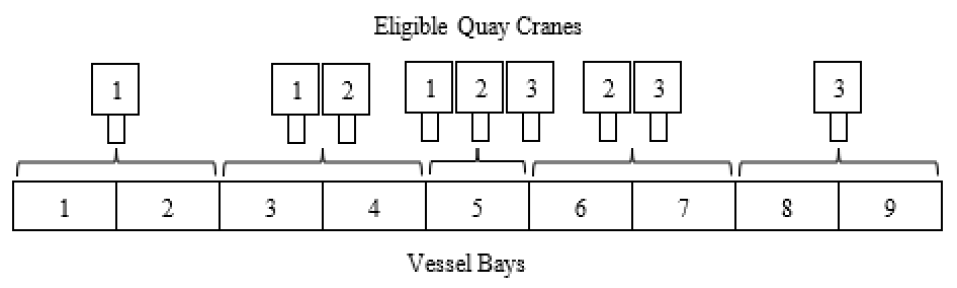
Figure 1: The Vessel Bays and Their Available QCs.

The main objective of a container terminal is to maximize total profit by increasing productivity. Terminal operators try to lower vessel turn times and decrease dwell times. To lower vessel turn times, the crane operations must be well-coordinated and the storage location of the inbound shipments must be chosen carefully, since they impact the distance traveled by the YTs. Therefore, the IPCTP jointly considers the storage location assignment for the inbound shipments from multiple berthed vessels and the crane assignment and scheduling for both outbound and inbound containers. The objective of the problem is to minimize the sum of weighted completion times of the vessels.

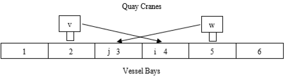
Figure 2: An Example of Interference for Shipments $i,j$ and Quay Cranes $v,w$.

The input parameters of the IPCTP are given in Table 1. Most are self-explanatory but some necessitate additional explanation. The smallest distance $\delta_{v,w}$ between quay cranes $v$ and $w$ is given by $\delta_{v,w}=\left(\delta+1\right)\left|v-w\right|$ where $\delta$ is the safety distance. The minimum time between the starting times of shipments $i$ and $j$ when processed by cranes $v$ and $w$ is given by

$$\Delta_{i,j}^{v,w}=\begin{cases}\left(b_{i}-b_{j}+\delta_{v,w}\right)s_{QC}&\mbox{if }v<w\mbox{ and }i\neq j\mbox{ and }b_{i}>b_{j}-\delta_{v,w}\\ \left(b_{j}-b_{i}+\delta_{v,w}\right)s_{QC}&\mbox{if }v>w\mbox{ and }i\neq j\mbox{ and }b_{i}<b_{j}-\delta_{v,w}\\ 0&\mbox{otherwise.}\end{cases}$$

This captures the time needed for a quay crane to travel to a safe distance in case of potential interference. This is illustrated in Figure 2. If shipments $i$ and $j$ are processed by cranes $v$ and $w$, then their starting times must be separated by $s_{QC}$ time units in order to respect the safety constraints (assuming that $w=v+1$). For instance, if shipment $i$ is processed first, crane $v$ must move to bay $1$ before shipment $j$ can be processed. Finally, the set of interferences can be defined by

$$\Theta=\{(i,j,v,w)\in C^{2}\times QC^{2}\mid i<j\ \&\ \Delta_{i,j}^{v,w}>0\}.$$

The dummy (initial and last) shipments are only used in the MIP model.

Table 1: The Parameters of the IPCTP.

$S$	Set of berthed vessels
$C_{u}^{s}$	Set of inbound shipments that belong to vessel $s\in S$
$C_{l}^{s}$	Set of outbound shipments that belong to vessel $s\in S$
$C$	Set of all shipments
$C_{u}$	Set of inbound shipments
$C_{l}$	Set of outbound shipments
$L_{u}$	Set of available yard locations for inbound shipments
$L_{l}$	Set of yard locations for outbound shipments
$l_{i}$	Yard location of outbound shipment $i\in C_{l}$
$L$	Set of all yard locations
$QC$	Set of QCs
$YC$	Set of YCs
$B$	Set of vessel bays
$B_{T}$	Total number of vessel bays
$QC_{T}$	Total number of QCs
$b_{i}$	Vessel bay position of shipment $i\in C$
$QC(i)$	Set of eligible QCs for shipment $i\in C$
$YC(k)$	The YC responsible for yard location $k\in L$
$w_{s}$	Weight (priority) of vessel $s\in S$
$Q_{i}$	QC handling time of shipment $i\in C$
$Y_{i}$	YT handling time of shipment $i\in C$
$tyt_{i}$	YT handling time of outbound shipment $i\in C_{l}$
$tt_{k}$	YT transfer time of inbound shipment to yard location $k\in L_{u}$
$tyc_{k,l}$	YC travel time between yard locations $k$ and $l$
$eqc_{i,j}$	QC travel time from shipment $i\in C$ to shipment $j\in C$
$eyc_{i,j}$	YC travel time from yard location $i\in L$ to yard location $j\in L$
$s_{QC}$	Travel time for unit distance of equipment $QC$
$\delta$	Safety distance between two $QC$s
$\delta_{v,w}$	Smallest allowed difference between bay positions of quay cranes $v$ and $w$
$\Delta_{i,j}^{v,w}$	Minimum time between the starting times of shipments $i$ and $j$
	when processed by cranes $v$ and $w$
$\Theta$	Set of all combinations of shipments and QCs with potential interferences
$0$	Dummy initial shipment
$N$	Dummy last shipment
$C^{0}$	Set of all shipments including dummy initial shipment $C\cup\{0\}$
$C^{N}$	Set of all shipments including dummy last shipment $C\cup\{N\}$
$M$	A sufficiently large constant integer

3 Literature Review

Port container terminal operations have received significant attention and many studies are dedicated to the sub-problems described earlier: See [1] for a classification of these subproblems. Recent work often consider the integration of two or three problems but very few papers propose formulations covering all the sub-problems jointly. Some papers give mathematical formulations of integrated problems but only use heuristic approaches given the computational complexity of solving the models. This section reviews recent publications addressing the integrated problems and highlights their contributions.

Chen et al. [3] propose a hybrid flowshop scheduling problem (HFSP) to schedule QCs, YTs, and YCs jointly. Both outbound and inbound operations are considered, but outbound operations only start after all inbound operations are complete. In the proposed mathematical model, each stage of the flowshop has unrelated multiple parallel machines and a tabu-search algorithm is used to address the computational complexity. Zheng et al. [22] study the scheduling of QCs and YCs, together with the yard storage and vessel stowage plans. The authors consider an automated container handling system, in which twin 40’ QCs and a railed container handling system is used. A rough yard allocation plan is maintained to indicate which blocks are available for storing the outbound containers from each bay. No mathematical model is provided, and the yard allocation, vessel stowage, and equipment scheduling is performed using a rule-based heuristic.

Xue et al. [21] propose a mixed integer programming (MIP) model for integrating the yard location assignment for inbound containers, quay crane scheduling, and yard truck scheduling. Non-crossing constraints and safety distances between QCs are ignored, and the assignment of QCs and YTs are predetermined. The yard location assignment considers block assignments instead of container slots. The resulting model cannot be solved for even medium-sized problems. Instead, a two-stage heuristic algorithm is employed, combining an ant colony optimization algorithm, a greedy algorithm, and local search.

Chen et al. [5] consider the integration of quay crane scheduling, yard crane scheduling, and yard truck transportation. The problem is formulated as a constraint-programming model that includes both equipment assignment and scheduling. However, non-crossing constraints and safety margins are ignored. The authors state that large-scale instances are computationally intractable for constraint programming and that even small-scale instances are too time-consuming. A three-stage heuristic algorithm is solved iteratively to obtain solutions for large-scale problems with up to 500 containers.

Wu et al. [18] study the scheduling of different types of equipment together with the storage strategy in order to optimize yard operations. Only loading operations for outbound containers are considered, and the tasks assigned to each QC and their processing sequence are assumed to be known. The authors formulate models to schedule the YCs and automated guided vehicles (AGV), and use a genetic algorithm to solve large-scale problems.

Homayouni et al. [6] study the integrated scheduling of cranes, vehicles, and storage platforms at automated container terminals. They consider a split-platform/retrieval system (SP-AS/RS), which includes AGVs and handling platforms for storing containers efficiently and providing quick access. A mathematical model of the same problem is proposed in [7]. In these studies, both outbound and inbound operations are considered. The origin and destination points of the containers are assumed to be predetermined and, in addition, empty for inbound containers. The earlier study proposes a simulated annealing (SA) algorithm to solve the problem, whereas the latter proposes a genetic algorithm (GA) outperforming SA under the same assumptions.

Lu and Le [12] propose an integrated optimization of container terminal scheduling, including YTs and YCs. The authors consider uncertainty factors such as YT travel speed, YC speed, and unit time of the YC operations. The assignment of YTs and YCs are not considered, and pre-assignments are assumed. The objective is to minimize the operation time of YCs in coordination with the YTs and QCs. The authors use a simulation of the real terminal operation environment to capture uncertainties. The authors also formulate a mathematical model and propose a particle swarm optimization (PSO) algorithm. As a future study, they indicate that the scheduling for simultaneous outbound and inbound operations should be considered for terminals adopting parallel operations.

Finally, a few additional studies [4, 8, 9, 10, 11, 14, 16, 19, 20] integrate different sub-problems, highlighting the increasing attention given to integrated solutions. They propose a wide range of heuristic or meta-heuristic algorithms; e.g., genetic algorithm, tabu search, particle swarm optimization, and rule-based heuristic methods.

Although most papers in container port operations focus on individual problems, recent developments have emphasized the need and potential for coordinating these interdependent operations. This paper pushes the state-of-the-art further by optimizing all operations holistically and demonstrating that constraint programming is a strong vehicle to address this integrated problem.

4 The MIP Model

Model 1 The MIP Model for the IPCTP: Decision Variables

Variables

$$x_{i,k}\in\{0,1\}:\mbox{inbound shipment }i\mbox{ is assigned to yard location }k$$

$$z_{i,j}^{q}\in\{0,1\}:\mbox{inbound shipment }j\mbox{ is handled immediately after shipment }i\mbox{ by QC }q$$

$$qz_{i,j}\in\{0,1\}:\mbox{inbound shipment }j\mbox{ is handled after shipment }i\mbox{ by QC }$$

$$v_{i,j}^{c}\in\{0,1\}:\mbox{ inbound shipment }j\mbox{ is handled immediately after shipment }i\mbox{ by YC }c$$

$$sqc_{i}\geq 0:\mbox{start time of shipment }i\mbox{ by its QC}$$

$$syc_{i}\geq 0:\mbox{start time of shipment }i\mbox{ by its YC}$$

$$t_{i}\geq 0:\mbox{travel time of YT for inbound shipment }i\mbox{ to assigned yard location }k$$

$$sy_{i,j}\geq 0:\mbox{travel time of YC from location }i\mbox{ to location }j$$

$$Cmax_{s}:\mbox{time of the last handled container at vessel }s$$

Model 2 The MIP Model for the IPCTP: Objective and Constraints

Objective

$$\mbox{minimize }\textstyle\sum_{s\in S}Cmax_{s}$$ (2a)

Constraints

$$Cmax_{s}\geq w_{s}\left(sqc_{i}+Q_{i}\right)\quad\forall s\in S,\forall i\in C_{l}^{s}\enspace$$ (2b)

$$Cmax_{s}\geq w_{s}\left(syc_{i}+Y_{i}\right)\quad\forall s\in S,\forall i\in C_{u}^{s}$$ (2c)

$$\textstyle\sum_{i\in C_{u}}x_{i,k}\leq 1\quad\forall k\in L_{u}$$ (2d)

$$\textstyle\sum_{k\in L_{u}}x_{i,k}=1\quad\forall i\in C_{u}$$ (2e)

$$\textstyle\sum_{j\in C^{N}}z_{0,j}^{q}=1\quad\forall q\in QC$$ (2f)

$$\textstyle\sum_{j\in C^{N}}v_{0,j}^{c}=1\quad\forall c\in YC$$ (2g)

$$\textstyle\sum_{j\in C^{0}}z_{i,N}^{q}=1\quad\forall q\in QC$$ (2h)

$$\textstyle\sum_{j\in C^{0}}v_{i,N}^{c}=1\quad\forall c\in YC$$ (2i)

$$\textstyle\sum_{q\in QC(i)}\sum_{j\in C^{N}}z_{i,j}^{q}=1\quad\forall i\in C,i\neq j$$ (2j)

$$\textstyle\sum_{j\in C^{N}}v_{i,j}^{YC(k)}=x_{i,k}\quad\forall k\in L_{u},\forall i\in C_{u},i\neq j$$ (2k)

$$\textstyle\sum_{j\in C^{N}}v_{i,j}^{YC(k)}=1\quad\forall k\in L_{l},\forall i\in C_{l},i\neq j$$ (2l)

$$\textstyle\sum_{j\in C^{0}}z_{j,i}^{q}-\sum_{j\in C^{N}}z_{i,j}^{q}=0\quad\forall i\in C,\forall q\in QC$$ (2m)

$$\textstyle\sum_{j\in C^{0}}v_{j,i}^{c}-\sum_{j\in C^{N}}v_{i,j}^{c}=0\quad\forall i\in C,\forall c\in YC$$ (2n)

$$\textstyle t_{i}=\sum_{k\in L_{u}}\left(tt_{k}*x_{i,k}\right)\quad\forall i\in C_{u}$$ (2o)

$$\textstyle sy_{i,j}=\sum_{m\in L_{u}}\left(tyc_{m,l_{i}}*x_{i,m}\right)\quad\forall i\in C_{u},\forall j\in C_{l}$$ (2p)

$$\textstyle sy_{i,j}=\sum_{m\in L_{u}}\sum_{l\in L_{u}}\left(tyc_{m,l}*x_{i,m}*x_{j,l}\right)\quad\forall i,j\in C_{u}$$ (2q)

$$\textstyle sy_{i,j}=\sum_{m\in L_{u}}\left(tyc_{l_{i},m}*x_{i,m}\right)\quad\forall i\in C_{l},\forall j\in C_{u}$$ (2r)

$$\textstyle sqc_{j}+M\left(1-z_{i,j}^{q}\right)\geq sqc_{i}+Q_{i}+eqc_{i,j}\quad\forall i,j\in C,\forall q\in QC$$ (2s)

$$\textstyle syc_{j}+M\left(1-v_{i,j}^{c}\right)\geq syc_{i}+Y_{i}+sy_{i,j}\quad\forall i\in C_{u},\forall j\in C,\forall c\in YC$$ (2t)

$$\textstyle syc_{j}+M\left(1-v_{i,j}^{c}\right)\geq syc_{i}+Y_{i}+sy_{i,j}\quad\forall i\in C_{l},\forall j\in C_{u},\forall c\in YC$$ (2u)

$$\textstyle syc_{j}+M\left(1-v_{i,j}^{c}\right)\geq syc_{i}+Y_{i}+eyc_{i,j}\quad\forall i,j\in C_{l},\forall c\in YC$$ (2v)

$$\textstyle sqc_{i}\geq syc_{i}+Y_{i}+tyt_{i}\quad\forall i\in C_{l}$$ (2w)

$$\textstyle syc_{i}\geq sqc_{i}+Q_{i}+t_{i}\quad\forall i\in C_{u}$$ (2x)

$$\textstyle sqc_{i}+Q_{i}-sqc_{j}\leq M\left(1-qz_{i,j}\right)\quad\forall i,j\in C$$ (2y)

$$\textstyle\sum_{u\in C^{0}}z_{u,i}^{v}+\sum_{u\in C^{0}}z_{u,j}^{w}\leq 1+qz_{i,j}+qz_{j,i}\quad\forall\left(i,j,v,w\right)\in\Theta$$ (2z)

$$\textstyle sqc_{i}+Q_{i}+\Delta_{i,j}^{v,w}-sqc_{j}\leq M\left(3-qz_{i,j}-\sum_{u\in C^{0}}z_{u,i}^{v}-\sum_{u\in C^{0}}z_{u,j}^{w}\right)\quad\forall\left(i,j,v,w\right)\in\Theta$$ (2aa)

The MIP decision variables are presented in Model 1, while the objective function and the constraints are given in Model 2. They use the formulation of QC interference constraints from [2].

The first set of MIP variables are binary: They determine the yard location of every inbound shipment and the (immediate) successor relationships on the cranes. The remaining variables are essentially devoted to the start times and the travel times of the shipments.

The objective function (2-01) minimizes the maximum weighted completion time of each vessel. Constraints (2-02–2-03) compute the weighted completion time of each vessel. Inbound shipments start their operations at a QC and finish at a YC, whereas outbound shipments follow the reverse order. Constraint (2-04) expresses that each available storage block stores at most one inbound shipment. Constraint (2-05) ensures that each inbound shipment is assigned an available storage block. All the containers of a shipment are assigned to the same block. Constraints (2-06–2-07) assigns the first (dummy) shipments to each QC and YC and Constraints (2-08–2-09) do the same for the last (dummy) shipments. Constraint (2-10) states that every shipment is handled by exactly one eligible QC. Constraints (2-11–2-12) ensures that each shipment is handled by a single YC. In Constraint (2-12), yard blocks are known at the beginning of the planning horizon for outbound shipments: They are thus directly assigned to the dedicated YCs. Constraints (2-13–2-14) guarantee that the shipments are handled in well-defined sequences by each handling equipment (QC and YC). Constraint (2-15) defines the YT transportation times for the inbounds shipments. Constraints (2-16–2-18) specify the empty travel times of the YCs according to yard block assignments of the shipments. Constraints (2-19–2-22) specify the relationship between the start times of two consecutive shipments processed by the same handling equipment. Constraints (2-23–2-24) are the precedence constraints for each shipment, which again differ for inbound and outbound shipments. Constraint (2-25) ensures that, if shipment $i$ precedes shipment $j$ on a QC, shipment $j$ cannot start its operation on that QC until shipment $i$ finishes. Constraint (2-26) guarantees that shipments that potentially interfere are not allowed to be processed at the same time on any QC. Constraint (2-27) imposes a minimum temporal distance between the processing of such shipments, which corresponds to the time taken by the QC to move to a safe location.

There are nonlinear terms in constraint (2-17), which computes the empty travel time of a YC, i.e., when it travels between the destinations of two inbound shipments. These terms can be linearized by introducing new binary variables of the form $\theta_{i,k,j,l}$ to denote whether inbound shipments $i,j\in C_{u}$ are assigned to yards locations $k,l\in L_{u}$. The constraints then become:

$$\textstyle sy_{i,j}=\sum_{k\in L_{u}}\sum_{l\in L_{u}}tyc_{k,l}\theta_{i,k,j,l}\quad\forall i,j\in C_{u}$$

$$\textstyle\theta_{i,k,j,l}\geq x_{i,k}+x_{j,l}-1,\forall i,j\in C_{u}\quad\forall k,l\in L_{u},i\neq j,k\neq l$$

$$\textstyle 2-\left(x_{i,k}+x_{j,l}\right)\leq 2\left(1-\theta_{i,k,j,l}\right)\quad\forall i,j\in C_{u},\forall k,l\in L_{u},i\neq j,k\neq l$$

5 The Constraint Programming Model

Model 3 The CP Model for the IPCTP

Variables

$$qc_{i}:\mbox{Interval variable for the QC handling of shipment }i$$

$$yt_{i}:\mbox{Interval variable for the YT handling of inbound shipment }i$$

$$aqc_{i,j}:\mbox{Optional interval variable for shipment }i\mbox{ on QC }j\mbox{ with duration }Q_{i}$$

$$ayc_{i,k}:\mbox{Optional interval variable for shipment }i\mbox{ on YC at yard location }k\mbox{ with duration }Y_{i}$$

$$qcs_{j}:\mbox{Sequence variable for QC }j\mbox{ over }\{aqc_{i,j}\mid i\in C\}$$

$$ycs_{j}:\mbox{Sequence variable for YC }j\mbox{ over }\{ayc_{i,k}\mid i\in C\wedge YC(k)=j\}$$

$$interfere_{i,v,j,w}:\mbox{Sequence variable over }\{aqc_{i,v},aqc_{j,w}\}$$

Objective

$$\mbox{minimize }\textstyle\sum_{s\in S}w_{s}\left(max\left(\max_{i\in C_{u}^{s}}\textsc{endOf}\left(yt_{i}\right),\max_{j\in C_{l}^{s}}\textsc{endOf}\left(qc_{j}\right)\right)\right)$$ (3a)

Constraints

$$\textstyle\textsc{alternative}\left(qc_{i},\mbox{all}\left(\mbox{$j$ in }QC\left(i\right)\right)aqc_{i,j}\right)\quad\forall i\in C\enspace$$ (3b)

$$\textstyle\textsc{alternative}\left(yt_{i},\mbox{all}\left(\mbox{$k$ in }L_{u}\right)ayc_{i,k}\right)\quad\forall i\in C_{u}$$ (3c)

$$\textstyle\sum_{i\in C_{u}}\textsc{presenceOf}\left(ayc_{i,k}\right)\leq 1\quad\forall k\in L_{u}$$ (3d)

$$\textstyle\textsc{presenceOf}\left(ayc_{i,l_{i}}\right)=1\quad\forall i\in C_{l}$$ (3e)

$$\textstyle\textsc{noOverlap}\left(ycs_{m},eyc_{i,j}\right)\quad\forall m\in YC$$ (3f)

$$\textstyle\textsc{noOverlap}\left(qcs_{m},eqc_{i,j}\right)\quad\forall m\in QC$$ (3g)

$$\textstyle\textsc{endBeforeStart}\left(aqc_{i,n},ayc_{i,k},tt_{k}\right)\quad\forall i\in C_{u},k\in L_{u},n\in QC_{i}$$ (3h)

$$\textstyle\textsc{endBeforeStart}\left(ayc_{i,l_{i}},aqc_{i,n},tyt_{i}\right)\quad\forall i\in C_{l},n\in QC_{i}$$ (3i)

$$\textstyle\textsc{noOverlap}\left(interfere_{i,v,j,w},\Delta_{i,j}^{v,w}\right)\ \forall i,j\in C,v\in QC_{i},w\in QC_{j}:\Delta_{i,j}^{v,w}>0$$ (3j)

The CP model is presented in Model 3 using the OPL API of CP Optimizer. It uses interval variables for representing the QC handling of all shipments and the YC handling of inbound shipments. In addition, a range of optional interval variables are used to represent the handling of shipment $i$ on QC $j$, and the handling of shipment $i$ at yard location $k$. The model also declares a number of sequence variables associated with each QC and YC: Each sequence constraint collects all the optional interval variables associated with a specific crane. Finally, the model declares a number of sequences for optional interval variables that may interfere.

The CP model minimizes the weighted completion time of each vessel by computing the maximum end date of the yard cranes (inbound shipments) and for the quay crane (outbound shipments). Alternative constraints (3-02) ensure that the QC processing of a shipment is performed by exactly one QC. Alternative constraints (3-03) enforce that each inbound shipment is allocated to exactly one yard location, and hence one yard crane. Constraints (3-04) state that at most one shipment can be allocated to each yard location. Constraints (3-05) fix the yard location (and hence the yard crane) of outbound shipments. Cranes are disjunctive resources and can execute only one task at a time, which is expressed by the noOverlap constraints (3-06–3-07) over the sequence variables associated with the cranes. These constraints also enforce the transition times between successive operations, capturing the empty travel times between yard locations (constraints 3-06) and bay locations (constraints 3-07). Constraints (3-08) impose the precedence constraints between the QC and YC tasks of inbound shipments, while adding the travel time to move the shipment from its bay to its chosen yard location. Constraints (3-09) impose the precedence constraints between the YC and QC operations of outbound shipments, adding the travel time from the fixed yard location to the fixed bay of the shipment. Interference constraints for the QCs are imposed by constraints (3-10). These constraints state that, if there is a conflict between two shipments and their QCs, then the two shipments cannot overlap in time, and their executions must be separated by a minimum time. This is expressed by noOverlap constraints over sequences consisting of the pairs of optional variables associated with these tasks.

6 Experimental Results

The MIP and CP models were written in OPL and run on the IBM ILOG CPLEX 12.7.1 software suite. The results were obtained on an Intel Core i7-5500U CPU 2.40 GHz computer.

6.1 Data Generation

The test cases were generated in accordance with earlier work, while capturing the operations of an actual container terminal. These are the first instances of this type, since the IPCTP has not been considered before in the literature. Travel and processing times in the test cases model those in the actual terminal. Different instances have slightly different times, as will become clear.

Figure 3 depicts the layout of the yard side considered in the experiments, which also models the actual terminal. The yard side is divided into 3 separate fields denoted by A, B, and C. Each field has two location areas and a single YC is responsible for each location area, giving a total of 6 yard cranes. In each location area, there are 2 yard block groups, shown as the dotted region, and traveling between them takes one unit of time. Field C is the nearest to the quay side, and there is a hill from field C to field A. The transportation times for YTs are generated according to these distances. YTs can enter and exit each field from the entrance shown in the figure, so the transfer times between the vessels and the yard blocks close to the entrance take less time. YT transfer times are generated between [5,10] considering the position of the yard blocks. At the quay side, the travel of a QC between consecutive vessel bay locations takes 3 units of time.

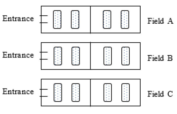
Figure 3: Layout of the Yard Side.

The processing times of the cranes for a single container are generated uniformly in [2,5] for YCs and [2,4] for QCs. The safety margin for the QCs is set to 1 vessel bay. The IPCTP is expressed in terms of shipments and the number of containers in each shipment is uniformly distributed between [4,40].

The experiments evaluate the impact of the number of shipments, the number of vessel bays, the inbound-outbound shipment ratio, and the number of available yard locations for inbound shipments. The number of shipments varies between 5 and 25, by increments of 5. The instances can thus contain up to 1,000 containers. The number of vessel bays are taken in $\{4,6,8\}$. The number of QCs depends on the vessel bays due to the QC restrictions: There are half as many QCs as there are vessel bays. The inbound-outbound shipment ratios are 20% and 50%, representing the fraction of inbound shipments over the outbound shipments. Finally, the number of available yard locations (U-L ratio) is computed from the number of inbound shipments: There are 2 to 3 times more yard locations than inbound shipments. For each configuration of the parameters, 5 random instances were generated.

6.2 Computational Results and Analysis

The Results

The results are given in Tables 2 and 3 for each configuration, for a total of 300 instances. Table 2 reports the results for 20% inbound-outbound ratio, and Table 3 for 50%. In the tables, each configuration is specified in terms of the U-L ratio, the number of bays and the number of shipments (Shp.). The average number of containers (Cnt.) in each shipment is also presented. For each such configuration, the tables report the average objective value and the average CPU time for its five instances. The CPU time is limited to an hour (3,600 seconds). The MIP solver did not always find feasible solutions within an hour for some or all five instances of a configuration. Note that this may result in an average objective value that is lower for the MIP model than the CP model, even when CP solves all instances optimally, since the MIP model may not find a feasible solution to an instance with a high optimal value. These cases are flagged by superscripts of the form $x/y$, where $x$ is the number of infeasible and $y$ is the number of suboptimal solutions in that average. The superscripts for CP indicate the number of suboptimal solutions. An entry ’NA’ in the table means that the MIP cannot find a feasible solution to any of the five instances. For the MIP, the tables also report the optimality gap on termination, i.e., the gap in percentage between the best lower and upper bounds.

For CP, the experiments were also run with a CPU limit of 600 seconds. The relative percentage deviations (RPD%) from the 1-hour runs are listed to assess CP’s ability to find high-quality solutions quickly. The RPD is computed as follows:

$$RPD\%=\dfrac{\left(\mbox{Obj. in 600 sec.}-\mbox{Obj. in 3600 sec.}\right)*100}{\left(\mbox{Obj. in 3600 sec.}\right)}.$$

Table 2: Results for Import-Export Rate 20%

				MIP			CP
U-L Ratio	# of Bays	# of Shp.	Avg. # of Cnt.	Obj.	CPU (sec.)	GAP%	Obj.	CPU (sec.)	RPD%
2	4	5	67.8	301.80	0.06	0.00	301.80	0.27	0.00
		10	88.8	$548.20^{0/3}$	3032.78	0.17	548.20	5.45	0.00
		15	99.8	$751.20^{0/5}$	3604.88	0.56	748.80	32.78	0.00
		20	117	$829.40^{0/5}$	3600.38	0.62	$820.00^{1}$	775.74	0.00
		25	139.4	$1032.75^{1/4}$	3600.25	0.66	$999.00^{2}$	1700.54	0.06
	6	5	157.2	242.00	0.06	0.00	242.00	0.34	0.00
		10	168.2	389.60	68.51	0.00	389.60	6.60	0.00
		15	193.4	$560.20^{0/5}$	3607.59	0.42	553.60	47.90	0.00
		20	207.8	$634.67^{2/3}$	3600.99	0.50	647.40	222.27	0.00
		25	233.8	$916.00^{4/1}$	3608.07	0.62	754.20	755.66	0.15
	8	5	246.8	584.00	0.13	0.00	583.90	1.18	0.00
		10	254.8	640.60	23.88	0.00	640.60	23.88	0.00
		15	279.4	$994.00^{0/5}$	3607.15	0.32	952.10	160.57	0.00
		20	306.2	$1261.00^{0/5}$	3600.63	0.45	1161.90	835.41	0.40
		25	325	NA	NA	NA	1343.10	1855.45	3385.58
3	4	5	338	244.40	0.09	0.00	244.40	0.33	0.00
		10	358.6	$434.00^{0/2}$	1488.63	0.10	434.00	5.10	0.00
		15	378.2	$642.40^{0/5}$	3604.06	0.49	641.20	38.15	0.00
		20	390.4	$863.80^{0/5}$	3603.24	0.64	$860.20^{1}$	840.29	0.00
		25	402.6	$920.00^{3/2}$	3625.08	0.65	$844.80^{2}$	2086.27	0.08
	6	5	418	310.20	0.22	0.00	310.20	0.45	0.00
		10	439	421.60	127.63	0.00	421.60	6.96	0.00
		15	461	$513.80^{0/5}$	3600.55	0.35	513.20	323.83	0.00
		20	484	$699.50^{3/2}$	3600.68	0.54	631.80	140.84	0.00
		25	509.4	$659.00^{4/1}$	3600.57	0.51	$856.80^{5}$	3601.78	0.14
	8	5	519.2	597.00	0.13	0.00	596.90	1.42	0.00
		10	532.8	815.40	161.25	0.00	815.20	25.67	0.00
		15	571.4	$980.40^{0/5}$	3600.70	0.30	972.40	232.30	0.00
		20	591.2	$1219.50^{3/2}$	3600.16	0.46	1214.90	1475.40	3.34
		25	611.2	$1471.00^{4/1}$	3600.27	0.48	$1449.50^{1}$	2498.82	4390.42

Table 3: Results for Import-Export Rate 50%

				MIP			CP
U-L Ratio	# of Bays	# of Shp.	Avg. # of Cnt.	Obj.	CPU (sec.)	GAP%	Obj.	CPU (sec.)	RPD%
2	4	5	67.8	320.40	0.21	0.00	320.40	0.47	0.00
		10	88.8	$541.60^{0/5}$	3600.08	0.37	541.60	15.93	0.00
		15	99.8	$738.40^{0/5}$	3600.97	0.58	738.40	113.76	0.00
		20	117	$755.67^{2/3}$	3600.31	0.60	$820.00^{1}$	1110.29	0.00
		25	139.4	$1570.00^{4/1}$	3600.63	0.77	$998.40^{2}$	1989.51	0.06
	6	5	157.2	199.00	0.11	0.00	199.00	0.83	0.00
		10	168.2	$377.00^{0/1}$	881.29	0.05	377.00	10.71	0.00
		15	193.4	$583.80^{0/5}$	3603.98	0.48	542.80	94.11	0.00
		20	207.8	$829.50^{3/2}$	3600.21	0.63	648.60	900.15	0.00
		25	233.8	$1811.00^{4/1}$	3600.52	0.81	$752.20^{1}$	1312.59	0.23
	8	5	246.8	580.40	0.22	0.00	580.20	2.36	0.00
		10	254.8	600.00	548.25	0.00	599.80	47.07	0.00
		15	279.4	$990.00^{1/4}$	3601.38	0.31	898.10	247.72	0.00
		20	306.2	$1149.33^{2/3}$	3600.35	0.38	1052.90	1323.69	3.64
		25	325	$3846.00^{3/2}$	3600.47	0.81	$1333.50^{4}$	3391.34	4559.78
3	4	5	338	265.00	0.22	0.00	265.00	0.95	0.00
		10	358.6	$428.40^{0/4}$	2893.00	0.23	428.40	18.07	0.00
		15	378.2	$653.50^{1/4}$	3601.66	0.49	$641.20^{1}$	813.17	0.00
		20	390.4	$1201.25^{1/4}$	3600.46	0.72	$859.80^{1}$	1230.81	0.00
		25	402.6	NA	NA	NA	$841.60^{5}$	3601.76	0.08
	6	5	418	302.40	0.61	0.00	302.40	1.21	0.00
		10	439	$407.80^{0/2}$	1777.30	0.13	407.80	16.12	0.00
		15	461	$488.00^{1/4}$	3607.27	0.33	$490.60^{1}$	855.09	0.00
		20	484	$971.33^{2/3}$	3600.57	0.65	$611.60^{1}$	959.72	0.00
		25	509.4	NA	NA	NA	$856.20^{5}$	3602.76	0.44
	8	5	519.2	550.80	0.18	0.00	550.50	2.57	0.00
		10	532.8	756.60	609.18	0.00	756.50	66.82	0.00
		15	571.4	$1006.20^{0/5}$	3600.69	0.33	968.80	427.87	0.00
		20	591.2	$2428.50^{3/2}$	3600.54	0.73	$1146.50^{1}$	2187.52	772.78
		25	611.2	NA	NA	NA	$1393.30^{5}$	3613.52	6479.76

MIP versus CP

The experimental results indicate that CP is orders of magnitude more efficient than MIP on the IPCTP. This is especially remarkable since this paper compares two black-box solvers. Overall, within the time limit, the MIP model does not find feasible solutions for 71 out of 300 instances and cannot prove optimality for 103 instances. On all but the smallest instances, the MIP solver cannot prove optimality for all five instances of the same confguration. In almost all configurations with 20 or more shipments, the MIP solver fails to find feasible solutions on at least one of the instances. In contrast, the CP model always find feasible solutions and proves optimality for 260 instances out of 300 instances. CP proves optimality on all but 12 instances in Table 3, and all but 28 in Table 2. On instances where both models find optimal solutions, the CP model is almost always 1–3 orders of magnitude faster (except for the smallest instances). Finally, the CP model always dominates the MIP model, in the sense that it proves optimality every time the MIP does.

Short Runs

On almost all instances but the largest ones, the CP model finds optimal, or near optimal, solutions within 10 minutes. On the largest instances, longer CPU times are necessary to find optimal or near-optimal solutions.

Sensitivity Analysis

The sensitivity analysis is restricted to the CP model for obvious reasons. The sensitivity of each factor is analyzed by comparing their respective run times and objective values. In general, the effect of the number of bays on the solution values and on CPU times tend to be small. In contrast, increasing the U-L ratio from 2 to 3 gives inbound shipments more alternatives for yard locations, which typically increases CPU times. Increasing the ratio of inbound-outbound containers also increases problem difficulty. This is not a surprise, since inbound shipments are more challenging, as they require a yard location assignment, while outbound shipments have both their yard locations and vessel bays fixed. Nevertheless, the CP model scales reasonably well when this ratio is increased. These analyses indicate that the number of shipments/containers is by far the most important element in determining the computing times in the IPCTP: The other factors have a significantly smaller impact, which is an interesting result in its own right.

7 Conclusion

This paper introduced the Integrated Port Container Terminal Problem (IPCTP) which, to the best of our knowledge, integrates for the first time, a wealth of port operations, including the yard location assignment, the assignment of quay and yard cranes, and the scheduling of these cranes under realistic constraints. In particular, the IPCTP considers empty travel time of the equipment and interference constraints between the quay cranes. The paper proposed both an MIP and a CP model for the IPCTP of a configuration based on an actual container terminal, which were evaluated on a variety of configurations regarding the number of vessel bays, the number of yard locations, the ratio of inbound-outbound shipments, and the number of shipments/containers. Experimental results indicate that the MIP model can only be solved optimally for small instances and often cannot find feasible solutions. The CP model finds optimal solutions for 87% of the instances and, on instances where both models can be solved optimally, the CP model is typically 1–3 orders of magnitude faster and proves optimality each time the MIP does. The CP model scales reasonably well with the number of vessel bays and yard locations, and the ratio of inbound-outbound shipments. It also solves large realistic instances with hundreds of containers. These results contrast with the existing literature which typically resort to heuristic or meta-heuristic algorithms, with no guarantee of optimality.

Future work will be devoted to capturing a number of additional features, including operator-based processing times, the stacking of inbound containers using re-shuffling operations, and the scheduling of the yard trucks.

References

- [1] Bierwirth, C., Meisel, F.: A follow-up survey of berth allocation and quay crane schedul-ing problems in container terminals. European Journal of Operational Research 244, 675–689 (2015)
- [2] Bierwirth, C., Meisel, F.: A fast heuristic for quay crane scheduling with interference constraints. Journal of Scheduling 12(4), 345–360 (2009)
- [3] Chen, L., Bostel, N., Dejax, P., Cai, J., Xi, L.: A tabu search algorithm for the integrated scheduling problem of container handling systems in a maritime terminal. European Journal of Operational Research 181, 40–58 (2007)
- [4] Chen, L., Bostel, N., Dejax, P., Cai, J., Xi, L.: A tabu search algorithm for the integrated scheduling problem of container handling systems in a maritime terminal. European Journal of Operational Research 181(1), 40 – 58 (2007)
- [5] Chen, L., Langevin, A., Lu, Z.: Integrated scheduling of crane handling and truck transportation in a maritime container terminal. European Journal of Operational Research 225(1), 142 – 152 (2013)
- [6] Homayouni, S.M., R Vasili, M., M Kazemi, S., H Tang, S.: Integrated scheduling of sp-as/rs and handling equipment in automated container terminals. In: Proceedings of International Conference on Computers and Industrial Engineering, CIE. vol. 2 (2012)
- [7] Homayouni, S.M., Tang, S.H., Motlagh, O.: A genetic algorithm for optimization of integrated scheduling of cranes, vehicles, and storage platforms at automated container terminals. Journal of Computational and Applied Mathematics 270(Supplement C), 545 – 556 (2014)
- [8] Homayouni, S., Tang, S.: Multi objective optimization of coordinated scheduling of cranes and vehicles at container terminals (2013)
- [9] Kaveshgar, N., Huynh, N.: Integrated quay crane and yard truck scheduling for unloading inbound containers. International Journal of Production Economics 159(Supplement C), 168 – 177 (2015)
- [10] Lau, H.Y., Zhao, Y.: Integrated scheduling of handling equipment at automated container terminals. International Journal of Production Economics 112(2), 665 – 682 (2008)
- [11] Liang, L., Lu, Z.Q., Zhou, B.H.: A heuristic algorithm for integrated scheduling problem of container handling system. In: 2009 International Conference on Computers Industrial Engineering. pp. 40–45. IEEE (2009)
- [12] Lu, Y., Le, M.: The integrated optimization of container terminal scheduling with uncertain factors. Computers & Industrial Engineering 75(Supplement C), 209 – 216 (2014)
- [13] Moccia, L., Cordeau, J.F., Gaudioso, M., Laporte, G.: A branch-and-cut algorithm for the quay crane scheduling problem in a container terminal. Naval Research Logistics (NRL) 53(1), 45–59 (2006)
- [14] Niu, B., Xie, T., Tan, L., Bi, Y., Wang, Z.: Swarm intelligence algorithms for yard truck scheduling and storage allocation problems. Neurocomputing 188(Supplement C), 284 – 293 (2016)
- [15] Sammarra, M., Cordeau, J.F., Laporte, G., Monaco, M.F.: A tabu search heuristic for the quay crane scheduling problem. Journal of Scheduling 10(4), 327–336 (2007)
- [16] Tang, L., Zhao, J., Liu, J.: Modeling and solution of the joint quay crane and truck scheduling problem. European Journal of Operational Research 236(3), 978 – 990 (2014)
- [17] Vis, I., de Koster, R.: Transshipment of containers at a container terminal: An overview. European Journal of Operational Research 147, 1–16 (2003)
- [18] Wu, Y., Luo, J., Zhang, D., Dong, M.: An integrated programming model for storage management and vehicle scheduling at container terminals. Research in Transportation Economics 42(1), 13 – 27 (2013)
- [19] Xin, J., Negenborn, R.R., Corman, F., Lodewijks, G.: Control of interacting machines in automated container terminals using a sequential planning approach for collision avoidance. Transportation Research Part C: Emerging Technologies 60(Supplement C), 377 – 396 (2015)
- [20] Xin, J., Negenborn, R.R., Lodewijks, G.: Energy-aware control for automated container terminals using integrated flow shop scheduling and optimal control. Transportation Research Part C: Emerging Technologies 44(Supplement C), 214 – 230 (2014)
- [21] Xue, Z., Zhang, C., Miao, L., Lin, W.H.: An ant colony algorithm for yard truck scheduling and yard location assignment problems with precedence constraints. Journal of Systems Science and Systems Engineering 22(1), 21–37 (2013)
- [22] Zheng, K., Lu, Z., Sun, X.: An effective heuristic for the integrated scheduling problem of automated container handling system using twin 40’ cranes. In: 2010 Second International Conference on Computer Modeling and Simulation. pp. 406–410. IEEE (2010)