First-order quantum phase transitions as condensations in the space of states

Abstract

We demonstrate that a large class of first-order quantum phase transitions, namely, transitions in which the ground state energy per particle is continuous but its first order derivative has a jump discontinuity, can be described as a condensation in the space of states. Given a system having Hamiltonian $H=K+gV$, where $K$ and $V$ are two non commuting operators acting on the space of states $\mathbb{F}$, we may always write $\mathbb{F}=\mathbb{F}_{\mathrm{cond}}\oplus\mathbb{F}_{\mathrm{norm}}$ where $\mathbb{F}_{\mathrm{cond}}$ is the subspace spanned by the eigenstates of $V$ with minimal eigenvalue and $\mathbb{F}_{\mathrm{norm}}=\mathbb{F}_{\mathrm{cond}}^{\perp}$. If, in the thermodynamic limit, $M_{\mathrm{cond}}/M\to 0$, where $M$ and $M_{\mathrm{cond}}$ are, respectively, the dimensions of $\mathbb{F}$ and $\mathbb{F}_{\mathrm{cond}}$, the above decomposition of $\mathbb{F}$ becomes effective, in the sense that the ground state energy per particle of the system, $\epsilon$, coincides with the smaller between $\epsilon_{\mathrm{cond}}$ and $\epsilon_{\mathrm{norm}}$, the ground state energies per particle of the system restricted to the subspaces $\mathbb{F}_{\mathrm{cond}}$ and $\mathbb{F}_{\mathrm{norm}}$, respectively: $\epsilon=\min\{\epsilon_{\mathrm{cond}},\epsilon_{\mathrm{norm}}\}$. It may then happen that, as a function of the parameter $g$, the energies $\epsilon_{\mathrm{cond}}$ and $\epsilon_{\mathrm{norm}}$ cross at $g=g_{\mathrm{c}}$. In this case, a first-order quantum phase transition takes place between a condensed phase (system restricted to the small subspace $\mathbb{F}_{\mathrm{cond}}$) and a normal phase (system spread over the large subspace $\mathbb{F}_{\mathrm{norm}}$). Since, in the thermodynamic limit, $M_{\mathrm{cond}}/M\to 0$, the confinement into $\mathbb{F}_{\mathrm{cond}}$ is actually a condensation in which the system falls into a ground state orthogonal to that of the normal phase, something reminiscent of Anderson’s orthogonality catastrophe (P. W. Anderson, Phys. Rev. Lett. 18, 1049 (1967)). The outlined mechanism is tested on a variety of benchmark lattice models, including spin systems, free fermions with non uniform fields, interacting fermions and interacting hard-core bosons.

• March 15, 2024

1 Introduction

Unlike classical phase transitions, which are based on a competition between entropy maximization and energy minimization, tuned by varying the temperature, quantum phase transitions (QPT) are characterized by a competition between two qualitatively different ground states (GSs) reachable by varying the Hamiltonian parameters at zero temperature [2, 3, 4, 5]. Typically, one has to compare the effects of two non commuting operators. To be specific, let us consider a lattice model with $N$ sites and $N_{\mathrm{p}}$ particles described by a Hamiltonian

$$H=K+gV,$$ (1)

where $K$ and $V$ are Hermitian non commuting operators, and $g$ a free dimensionless parameter. One can represent $H$ in the eigenbasis of $V$. In such a case, it is natural to call $V$ a “potential” operator, and $K$ a “hopping” operator. Let us suppose that both $K$ and $V$ scale linearly with the number of particles $N_{\mathrm{p}}$. Since in the two opposite limits $g\to 0$ and $g\to\infty$, the GS of the system tends to the GS of $K$ and $V$, respectively, one wonders if, in the thermodynamic limit, a QPT takes place at some intermediate critical value of $g$: $g_{\mathrm{c}}=O(1)$. In fact, an argument based on the “avoided-crossing-levels” [6] suggests that a possible abrupt bending of the GS energy of $H$ occurs. However, there is no exact way to apply this scheme and, by varying $g$, three possibilities remain open: i) there is no QPT; ii) there exists a $g_{\mathrm{c}}$ where a second-order transition takes place; iii) there exists a $g_{\mathrm{c}}$ where the first derivative of the GS energy makes a finite jump. Let us discuss briefly these scenarios.

i) Here we mention only that, in principle, there could be no QPT at all, or even a QPT with no singularity [5].

ii) Within some extent, Landau’s theory of classical critical phenomena offers a universal approach also to second-order QPTs via the quantum-classical mapping, according to which the original quantum model in $d$ dimensions is replaced by an effective classical system in $d+z$ dimensions [7, 2, 5], $z$ being the dynamical critical exponent. Hence, for second-order QPTs, concepts and tools originally defined for classical critical phenomena find a quantum counterpart and the main issue concerns the competition between classical and quantum fluctuations.

iii) A different situation occurs for first-order QPTs for which a universal mechanism seems lacking [8]. As for the classical case, first-order QPTs can result from the finite jump of the order parameter when crossing the coexistence line of two different phases that originate from the same critical point of a second-order transition [9]. Notice that, for such a scenario to occur at zero temperature, one needs that $H$ (or the corresponding Lagrangian) depends on at least two independent parameters (say $g_{1}$ and $g_{2}$). In these first-order transitions, universality reflects on finite size scaling [10]. Some kind of universality of first-order QPTs is expected also in systems of vector spin models with a sufficiently large number of components, as in the 1D quantum Potts model [11]. In general, however, for genuine first-order QPTs driven by a single parameter $g$, i.e., those that do not originate from the critical point of a second-order transition (as, e.g., in the case of frustrated [12], mean-field, and random spin systems [13, 14, 15, 16]), or those for which there is no evident classical analog, it is not clear which universal mechanism, if any, is at their basis. Lack of universality has been in fact observed in the gap $\Delta$ (the difference between the two lowest energy levels) of certain systems [17]. In some cases $\Delta$ does not take the absolute minimum at $g_{\mathrm{c}}$ (see A.2). There are even systems where $\Delta$ remains finite, as in certain topological second-order [18, 19] and first-order [20, 21] QPTs.

In this paper, we test a theory concerning a large class of first-order QPTs that lead to many-body condensation thorough a counter-intuitive mechanism having no classical analog and that can be interpreted as a many-body Anderson’s orthogonality catastrophe [1]. The approach provides also an efficient criterion for localizing the critical point. We first formulate the theory in general terms, regardless of the details of $K$ and $V$ (where we allow for the presence of also more than one parameter), then we test it on several specific models: spin systems, free fermions in a heterogeneous external field, interacting fermions and interacting hard-core bosons, with both open and periodic boundary conditions. A comparison with the fidelity method [22] is also discussed. The paper is equipped with Appendices that illustrate some immediate extensions of the theory and provide further critical checks. Here, we discuss our theory at zero temperature while its finite temperature counterpart will be reported elsewhere.

2 Main result

Consider a system with Hamiltonian as in Eq. (1), and let $\{|n\rangle\}$ be a complete orthonormal set of eigenstates of $V$: $V|n\rangle=V_{n}|n\rangle$, $n=1,\dots,M$. We assume ordered potential values $V_{1}\leq V_{2}\leq\dots\leq V_{M}$. Let $M_{\mathrm{cond}}$ be the degeneracy of the smallest potential $V_{\mathrm{min}}=V_{1}=V_{2}=\dots=V_{M_{\mathrm{cond}}}$. The Hilbert space of the system, $\mathbb{F}=\mathrm{span}\{|n\rangle\}_{n=1}^{M}$, equipped with standard complex scalar product $\langle u|v\rangle$, can be decomposed as the direct sum $\mathbb{F}=\mathbb{F}_{\mathrm{cond}}\oplus\mathbb{F}_{\mathrm{norm}}$, where $\mathbb{F}_{\mathrm{cond}}=\mathrm{span}\{|n\rangle\}_{n=1}^{M_{\mathrm{cond}}}$ and $\mathbb{F}_{\mathrm{norm}}=\mathrm{span}\{|n\rangle\}_{n=M_{\mathrm{cond}}+1}^{M}=\mathbb{F}_{\mathrm{cond}}^{\perp}$. Any vector $|u\rangle\in\mathbb{F}$ can be uniquely written as $|u\rangle=|u_{\mathrm{cond}}\rangle+|u_{\mathrm{norm}}\rangle$, where $|u_{\mathrm{cond}}\rangle\in\mathbb{F}_{\mathrm{cond}}$ and $|u_{\mathrm{norm}}\rangle\in\mathbb{F}_{\mathrm{cond}}^{\perp}$. Finally, we define

$$E=\inf_{|u\rangle\in\mathbb{F}}\frac{\langle u|H|u\rangle}{\langle u|u\rangle}$$

$$E_{\mathrm{cond}}=\inf_{|u\rangle\in\mathbb{F}_{\mathrm{cond}}}\frac{\langle u|H|u\rangle}{\langle u|u\rangle},$$

$$E_{\mathrm{norm}}=\inf_{|u\rangle\in\mathbb{F}_{\mathrm{norm}}}\frac{\langle u|H|u\rangle}{\langle u|u\rangle}.$$

Clearly, $E$ is the GS energy of the system and by construction $E\leq\min\{E_{\mathrm{cond}},E_{\mathrm{norm}}\}$. Less trivial is to understand the relation among $E$, $E_{\mathrm{cond}}$ and $E_{\mathrm{norm}}$ in the thermodynamic limit.

To properly analyze this limit, let us consider systems consisting of $N_{\mathrm{p}}$ particles in a lattice with $N$ sites and assume that the lowest eigenvalues of $K$ and $V$ scale linearly with $N_{\mathrm{p}}$, at least for $N_{\mathrm{p}}$ large. The thermodynamic limit is defined as the limit $N,N_{\mathrm{p}}\to\infty$ with $N_{\mathrm{p}}/N=\varrho$ constant. Because of the assumed scaling properties, the energies $E(N,N_{\mathrm{p}})$, $E_{\mathrm{cond}}(N,N_{\mathrm{p}})$ and $E_{\mathrm{norm}}(N,N_{\mathrm{p}})$ diverge linearly with the number of particles, therefore, if divided by $N_{\mathrm{p}}$, they have finite thermodynamic limits which depend on the chosen density $\varrho$. We call these limits $\epsilon(\varrho)$, $\epsilon_{\mathrm{cond}}(\varrho)$, and $\epsilon_{\mathrm{norm}}(\varrho)$ [23].

We state that, under the above scaling conditions on $K$ and $V$,

$$\mbox{if }\lim_{N,N_{\mathrm{p}}\to\infty,N_{\mathrm{p}}/N=\varrho}{M_{\mathrm{cond}}/M}=0,\qquad\mbox{then }\epsilon(\varrho)=\min\{\epsilon_{\mathrm{cond}}(\varrho),\epsilon_{\mathrm{norm}}(\varrho)\}.$$ (2)

Equation (2) establishes the possibility of a QPT between a normal phase characterized by the energy per particle $\epsilon_{\mathrm{norm}}$, obtained by removing from $\mathbb{F}$ the infinitely smaller sub-space $\mathbb{F}_{\mathrm{cond}}$, and a condensed phase characterized by the energy per particle $\epsilon_{\mathrm{cond}}$ obtained by restricting the action of $H$ onto $\mathbb{F}_{\mathrm{cond}}$. Note that the Hilbert space dimension $M(N,N_{\mathrm{p}})$ diverges, generally in an exponential way, with $N$ and $N_{\mathrm{p}}$. The dimension $M_{\mathrm{cond}}$ may or may not be a growing function of $N$ and $N_{\mathrm{p}}$. In any case, if $M_{\mathrm{cond}}/M\to 0$, in the space of the Hamiltonian parameters the equation

$$\epsilon_{\mathrm{norm}}(\varrho)=\epsilon_{\mathrm{cond}}(\varrho),$$ (3)

provides the coexistence surface of two phases, crossing which a QPT takes place. If $H$ depends on a single parameter $g$, as in Eq. (1), the coexistence surface reduces to a critical point $g_{\mathrm{c}}$, which is given as the minimal solution, if any, of Eq. (3) (in general, $\epsilon_{\mathrm{norm}}$ and $\epsilon_{\mathrm{cond}}$ can be equal also for $g\neq g_{\mathrm{c}}$). In virtue of Eq. (3), the transition is first-order. In fact, $\epsilon_{\mathrm{norm}}$ and $\epsilon_{\mathrm{cond}}$ correspond to the lowest eigenvalues of two different matrix Hamiltonians so that, as functions of the Hamiltonian parameters, they are different, except possibly for a finite number of crossing points solution of Eq. (3). Assuming that $\epsilon_{\mathrm{norm}}$ and $\epsilon_{\mathrm{cond}}$ are both everywhere analytic, implies that their first derivatives around any crossing point are, in general, also different. This is quite clear when there is only one Hamiltonian parameter: given two analytic functions of one variable, either they coincide everywhere, or their first derivatives at the crossing points (if any) are different. According to Ehrenfest classification this means that the QPT is of first-order.

Equations (2-3) are quite general. Whereas the paradigm of second-order QPTs looks for changes of symmetries of the GS, the paradigm of the first-order QPTs determined by Eqs. (2-3) looks for condensations of the GS into $\mathbb{F}_{\mathrm{cond}}$ (which may be accompanied by a broken symmetry or not). The word “condensation” here refers to the fact that, in the condensed phase, thanks to the condition $M_{\mathrm{cond}}/M\to 0$, the GS occupies an infinitesimal portion of the full space of states. Depending on the structure of the space $\mathbb{F}_{\mathrm{cond}}$, this abstract condensation in the Hilbert space can have different physical manifestations. As we shall show by specific examples, in certain cases the condensation can realize through a partial or total freezing of the particles, and even as an actual localization of matter. Such condensations were first demonstrated in [14] for two classes of models, the uniformly fully connected models and the random potential systems. For general systems, a formal proof based on the concept of sojourn times in the subspaces $\mathbb{F}_{\mathrm{cond}}$ and $\mathbb{F}_{\mathrm{norm}}$ is given in [24]. Here, we provide a simple algebraic argument which goes as follows. We start with the obvious inequality $\epsilon\leq\min\{\epsilon_{\mathrm{cond}},\epsilon_{\mathrm{norm}}\}$, and demonstrate that the opposite inequality holds too. Let us evaluate $\epsilon$ as the thermodynamic limit of

$$\frac{1}{N_{\mathrm{p}}}\inf_{|u\rangle\in\mathbb{F}}\frac{\langle u|H|u\rangle}{\langle u|u\rangle}$$

$$\qquad=\frac{1}{N_{\mathrm{p}}}\inf_{0\leq x\leq 1}\inf_{|u_{\mathrm{cond}}\rangle\in\mathbb{F}_{\mathrm{cond}}}\inf_{|u_{\mathrm{norm}}\rangle\in\mathbb{F}_{\mathrm{norm}}}\biggl{(}\frac{\langle u_{\mathrm{cond}}|H|u_{\mathrm{cond}}\rangle}{\langle u_{\mathrm{cond}}|u_{\mathrm{cond}}\rangle}x+\frac{\langle u_{\mathrm{norm}}|H|u_{\mathrm{norm}}\rangle}{\langle u_{\mathrm{norm}}|u_{\mathrm{norm}}\rangle}(1-x)$$

$$\qquad\qquad+\frac{\mathop{\rm Re}\langle u_{\mathrm{cond}}|K|u_{\mathrm{norm}}\rangle}{\sqrt{\langle u_{\mathrm{cond}}|u_{\mathrm{cond}}\rangle\langle u_{\mathrm{norm}}|u_{\mathrm{norm}}\rangle}}2\sqrt{x(1-x)}\biggr{)},$$ (4)

where $|u\rangle=|u_{\mathrm{cond}}\rangle+|u_{\mathrm{norm}}\rangle$ with $\langle u_{\mathrm{cond}}|u_{\mathrm{norm}}\rangle=0$ and $x=\langle u_{\mathrm{cond}}|u_{\mathrm{cond}}\rangle/\langle u|u\rangle$. We find

$$\epsilon\geq\inf_{0\leq x\leq 1}\left(\epsilon_{\mathrm{cond}}x+\epsilon_{\mathrm{norm}}(1-x)+\beta 2\sqrt{x(1-x)}\right),$$ (5)

where $\beta$ is the thermodynamic limit of $B/N_{\mathrm{p}}$ and

$$B=\inf_{|u_{\mathrm{cond}}\rangle\in\mathbb{F}_{\mathrm{cond}}}\inf_{|u_{\mathrm{norm}}\rangle\in\mathbb{F}_{\mathrm{norm}}}\allowbreak\mathop{\rm Re}\langle u_{\mathrm{cond}}|K|u_{\mathrm{norm}}\rangle/\sqrt{\langle u_{\mathrm{cond}}|u_{\mathrm{cond}}\rangle\langle u_{\mathrm{norm}}|u_{\mathrm{norm}}\rangle}.$$ (6)

Let $|\tilde{u}_{\mathrm{cond}}\rangle=\sum_{n=1}^{M_{\mathrm{cond}}}c_{n}|n\rangle$ and $|\tilde{u}_{\mathrm{norm}}\rangle=\sum_{n=M_{\mathrm{cond}}+1}^{M}d_{n}|n\rangle$ be the states of $\mathbb{F}_{\mathrm{cond}}$ and $\mathbb{F}_{\mathrm{norm}}$ which realize this double infimum. We now prove that $\beta=0$. Suppose, for simplicity, that $K$ is the sum of $N_{\mathrm{p}}$ single-particle jump operators, i.e., $\langle n|K|m\rangle=-1$ if $m$ is one of the $N_{\mathrm{p}}$ configurational states first neighbor to $n$, and zero otherwise. We estimate

$$\frac{|B|}{N_{\mathrm{p}}}\leq\frac{1}{N_{\mathrm{p}}}\sum_{n=1}^{M_{\mathrm{cond}}}\sum_{m=M_{\mathrm{cond}}+1}^{M}\left|c_{n}\right|\left|d_{m}\right|\left|\langle n|K|m\rangle\right|\sim\sqrt{\frac{M_{\mathrm{cond}}}{M}}$$

provided that, as we expect normalizing the states $|\tilde{u}_{\mathrm{cond}}\rangle$ and $|\tilde{u}_{\mathrm{norm}}\rangle$ to 1, $\left|c_{n}\right|\sim 1/\sqrt{M_{\mathrm{cond}}}$ and $\left|d_{m}\right|\sim 1/\sqrt{M-M_{\mathrm{cond}}}$. If, in the thermodynamic limit, $M_{\mathrm{cond}}/M\to 0$, it follows that $\beta=0$ and Eq. (5) gives $\epsilon\geq\min\{\epsilon_{\mathrm{cond}},\epsilon_{\mathrm{norm}}\}$.

When $\min\{E_{\mathrm{cond}},E_{\mathrm{norm}}\}$ becomes, for $N,N_{\mathrm{p}}$ finite but increasing, closer and closer to $E$, $\max\{E_{\mathrm{cond}},E_{\mathrm{norm}}\}$ provides, although only close to the critical point, a good approximation to $E^{\prime}$, the energy of the first excited state of $H$. Whereas $E^{\prime}$ is difficult to evaluate numerically, $E_{\mathrm{cond}}$ and $E_{\mathrm{norm}}$, which are both defined as GS energies of the system restricted to $\mathbb{F}_{\mathrm{cond}}$ and $\mathbb{F}_{\mathrm{norm}}$, are a much easier target, specially in Monte Carlo simulations (MCSs). We therefore define [23]

$$\Delta_{0}=\left|E_{\mathrm{cond}}-E_{\mathrm{norm}}\right|,$$ (7)

whose minimum allow us to locate in a simple way the critical point when $N,N_{\mathrm{p}}$ are large enough. However, in the cases in which $\epsilon_{\mathrm{norm}}$ and $\epsilon$ overlap for all $g$ in some interval (eventually infinite), rather than to cross just at $g_{\mathrm{c}}$, it is convenient to locate $g_{\mathrm{c}}$ by analyzing

$$\Delta_{1}=|E_{\mathrm{cond}}-E|.$$ (8)

When possible, we compare $\Delta_{0}$ and $\Delta_{1}$ with $\Delta=E^{\prime}-E$, the ordinary gap. Notice that, in general, according to Eq. (2), only $\Delta_{0}/N_{\mathrm{p}}$ and $\Delta_{1}/N_{\mathrm{p}}$ vanish at $g=g_{\mathrm{c}}$. However, a plot of $\Delta_{0}$ and $\Delta_{1}$ effectively allows for a precise localization of $g_{\mathrm{c}}$.

In the following, we test Eqs. (2-3) on several models by means of numerical diagonalizations (NDs) and MCSs [25]. The approach to the thermodynamic limit is studied by increasing the size $N$ with $N_{\mathrm{p}}=\varrho N$ and $\varrho$ fixed.

3 Grover Model

Let us consider a set of $N$ spins with Hamiltonian

$$H=-\sum_{i=1}^{N}\sigma_{i}^{x}-gN\bigotimes_{i=1}^{N}\frac{1-\sigma_{i}^{z}}{2},$$ (9)

where $\sigma_{i}^{x}$ and $\sigma_{i}^{z}$ are the Pauli matrices acting on the $i$-th spin. In this model, in which $N_{\mathrm{p}}=N$, we have $M=2^{N}$ and $\mathbb{F}=\mathrm{span}\{|s_{1}\rangle\otimes\dots\otimes|s_{N}\rangle\}$, where $|s_{i}\rangle$, with $s_{i}=\pm 1$, are the eigenstates of $\sigma_{i}^{z}$. Equation (9) is of interest as a benchmark model in quantum information theory, and corresponds to the quantum version of the classical search problem [26, 27], where a single target state must be found over a set of $M$ unstructured states. Notice that no efficient MCSs exist for this model, the form of the potential being the worst case scenario for any hypothetical importance sampling [28]. The model is also of interest to quantum adiabatic algorithms [29]. In [14] we solved a random version of (9), where the second term of $H$ is built by randomly assigning the value $-gN$ to a single state of $\mathbb{F}$ and a quenched average over many independent realizations is taken at the end. The present non-random model provides the simplest paradigmatic example that illustrates the role and the validity of Eqs. (2-3).

Comparing Eq. (9) with Eq. (1), we see that $K=-\sum_{i}\sigma_{i}^{x}$ and $V=-N\otimes_{i=1}^{N}(1-\sigma_{i}^{z})/2$. The potential $V$ has its minimal eigenvalue in correspondence with the state $|1\rangle\equiv|s_{1}=-1\rangle\otimes\dots\otimes|s_{N}=-1\rangle$, namely, $V_{\mathrm{min}}=V_{1}=-N$, whereas $V_{n}=0$ for $n=2,\dots,M$. We thus have $M_{\mathrm{cond}}=1$, $\mathbb{F}_{\mathrm{cond}}=\mathrm{span}\{|1\rangle\}$, $E_{\mathrm{cond}}=-gN$ and $\epsilon_{\mathrm{cond}}=-g$. Consider now the GS of $H$ in $\mathbb{F}_{\mathrm{norm}}=\mathbb{F}_{\mathrm{cond}}^{\perp}$. For $N$ finite, we are not able to analytically calculate $E_{\mathrm{norm}}$. However, we observe that, since $|1\rangle\notin\mathbb{F}_{\mathrm{norm}}$, $E_{\mathrm{norm}}$ cannot depend on $g$. Hence, for $E_{\mathrm{norm}}$ there is no QPT and we can apply Eq. (2) to obtain $\epsilon_{\mathrm{norm}}=\lim_{N\to\infty}E(g=0)/N=-1$. In conclusion,

$$M_{\mathrm{cond}}/M=2^{-N},\qquad\epsilon_{\mathrm{cond}}=-g,\qquad\epsilon_{\mathrm{norm}}=-1,$$ (10)

and applying Eq. (2) we find

$$\epsilon=\left\{\begin{array}[]{l}-1,\qquad g<1,\\ -g,\qquad g\geq 1.\end{array}\right.$$ (13)

Figure 1(a) shows the results from NDs. As $N$ grows, the GS energy per spin tends to the curve $\epsilon$, predicted by Eq. (13), with a finite discontinuity in its first derivative at $g_{\mathrm{c}}=1$. Figure 1(a) also shows that, as $N$ increases, $\Delta(g)$ and $\Delta_{0}(g)$ take their minima at $g$ closer and closer to $g_{\mathrm{c}}$.

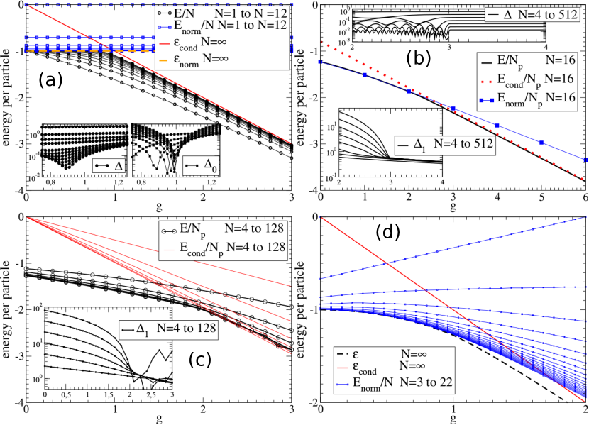
Figure 1: (a) GS energies per particle obtained from NDs, as a function of $g$, for the model described by Eq. (9). Circles: $E/N$ for $N=1$ to $12$ (lowest to highest plot), lines are guides for the eyes. Squares: $E_{\mathrm{norm}}/N$ for $N=1$ to $12$ (highest to lowest). The thermodynamic limits, Eqs. (10), are represented by straight lines, $\epsilon_{\mathrm{norm}}$ (thick horizontal dashed line), and $\epsilon_{\mathrm{cond}}$ (solid line), crossing at the critical point $g_{\mathrm{c}}=1$. Left Inset: gap $\Delta$ as a function of $g$, for $N=1$ to $12$ (highest to lowest). Right Inset: the function $\Delta_{0}$, Eq. (7), for $N=1$ to $12$ (about leftest to rightest). (b) GS energies per particle for the model of Eq. (14) with $N_{\mathrm{p}}=N/2$ and $N_{\mathrm{imp}}=N/4$. Upper Inset: gap $\Delta$, for $N=4,\dots,512$ via powers of 2 (highest to lowest). Lower Inset: the function $\Delta_{1}$, for $N=4,\dots,512$ via powers of 2 (highest to lowest). The curves $E_{\mathrm{cond}}/N_{\mathrm{p}}$ are obtained from Eq. (16) whereas $E_{\mathrm{norm}}/N_{\mathrm{p}}$ from MCSs. Here $g_{\mathrm{c}}\simeq 3$. (c): GS energies per particle for the model of Eq. (17) with $N_{\mathrm{p}}=N/2$ for $N=4,\dots,128$ via powers of 2 (highest to lowest). Solid lines: $E_{\mathrm{cond}}/N_{\mathrm{p}}$ from Eq. (18). Circles: $E/N_{\mathrm{p}}$ from MCSs. Inset: $\Delta_{1}$ for $N=4,\dots,128$ via powers of 2 (lowest to highest). Here $g_{\mathrm{c}}\simeq 2.0$. (d): GS energies per particle for the Ising model, Eq. (19): $\epsilon_{\mathrm{cond}}=-g$ (continuous line), $\epsilon$ (dashed line), $E_{\mathrm{norm}}/N$ (line with points) for $N$= 3 to 22 (top to bottom).

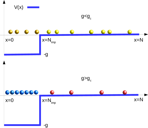
Figure 2: Pictorial view of the GS of the model given by Eq. (14) representing $N_{\mathrm{p}}$ free spinless electrons confined in a segment of length $N$ and in the presence of a non uniform external field. Here, the GS is the antisymmetrized product of $N_{\mathrm{p}}$ suitable single-particle states, each being eigenstate of a single-particle Hamiltonian with hopping operator $K$ and a step potential operator $V(x)$ characterized by a well of depth $g$ and length $N_{\mathrm{imp}}$. Top panel: For $g<g_{c}$ the GS is the antisymmetrized product of $N_{\mathrm{p}}$ quasi free electrons waves confined in the range $0\leq x\leq N$, with some slightly more localized than others in the range $0\leq x\leq N_{\mathrm{imp}}$ (sketched as light and dark yellow balls). Bottom panel: for $g>g_{c}$ the GS is the antisymmetrized product of $N_{\mathrm{p}}-N_{\mathrm{imp}}$ free electrons waves confined in the range $N_{\mathrm{imp}}<x\leq N$ (sketched as red balls) times the antisymmetrized product of $N_{\mathrm{imp}}$ frozen position states over the range $0\leq x\leq N_{\mathrm{imp}}$ (sketched as blue balls). Notice that using OBC or PBC does not affect the picture, see Appendix B for details.

4 Spinless fermions in 1D with a nonuniform external field

Let us consider $N_{\mathrm{p}}$ spinless fermions in a 1D chain of $N\geq N_{\mathrm{p}}$ sites with open boundary conditions (OBC). The advantage of choosing OBC stems from the fact that, for fermions in 1D, there is no sign-problem in MCSs [30]; in B we discuss the case of periodic boundary conditions (PBC). The Hamiltonian is

$$H=-\sum_{i=1}^{N-1}\left(c^{\dagger}_{i}c_{i+1}+c^{\dagger}_{i+1}c_{i}\right)-g\sum_{i=1}^{N_{\mathrm{imp}}}c^{\dagger}_{i}c_{i},$$ (14)

where $c_{i}$ are fermionic annihilation operators and $N_{\mathrm{imp}}\leq N_{\mathrm{p}}$ is the number of impurities, or the number of sites where an external field applies. For simplicity, we choose to have these impurities in the first $N_{\mathrm{imp}}$ sites of the chain. This choice is not restrictive but allows to calculate $\epsilon_{\mathrm{cond}}$ more easily. We consider the half-filling case $N_{\mathrm{p}}=N/2$ with $N$ even, so that $M=\binom{N}{N/2}$. Since $H$ is quadratic in the fermionic operators, the corresponding eigenvalue problem can be exactly solved by diagonalizing the associated $N\times N$ Toeplix matrix $\bm{A}$, whose non zero elements are $A_{i+1,i}=A_{i,i+1}=-1$, for $i=1,\dots,N-1$, and $A_{i,i}=-g$, for $i=1,\dots,N_{\mathrm{imp}}$. The eigenvalues of $\bm{A}$ are single particles energies, which, summed up according to Pauli’s principle, form the $N_{\mathrm{p}}$-particle eigenvalues of $H$. The matrix $\bm{A}$ can be numerically diagonalized for quite large sizes $N$ and we can evaluate the exact gap as a further benchmark of the theory.

For $N_{\mathrm{imp}}=N_{\mathrm{p}}$, the minimal potential occurs in correspondence with the single state $|1\rangle=c^{\dagger}_{1}c_{1}\dots c^{\dagger}_{N_{\mathrm{p}}}c_{N_{\mathrm{p}}}|\bm{0}\rangle$, where $|\bm{0}\rangle$ is the vacuum state and $V_{\mathrm{min}}=V_{1}=-N_{\mathrm{p}}$. For $N_{\mathrm{imp}}<N_{\mathrm{p}}$, instead, $V_{\mathrm{min}}$ is degenerate, and $\mathbb{F}_{\mathrm{cond}}$ spans those states in which $N_{\mathrm{imp}}$ fermions occupy the first $N_{\mathrm{imp}}$ sites. We have

$$M_{\mathrm{cond}}=\binom{N-N_{\mathrm{imp}}}{N_{\mathrm{p}}-N_{\mathrm{imp}}},$$ (15)

$$\frac{E_{\mathrm{cond}}}{N_{\mathrm{p}}}=-g\frac{N_{\mathrm{imp}}}{N_{\mathrm{p}}}+\frac{E^{(0)}\left({N-N_{\mathrm{imp}}},{N_{\mathrm{p}}-N_{\mathrm{imp}}}\right)}{N_{\mathrm{p}}},$$ (16)

where $E^{(0)}(N-N_{\mathrm{imp}},N_{\mathrm{p}}-N_{\mathrm{imp}})$ is the GS energy of a system of $N_{\mathrm{p}}-N_{\mathrm{imp}}$ free spinless fermions in a 1D lattice of $N-N_{\mathrm{imp}}$ sites with OBC, whose single-particle energies are $e^{(0)}_{l}=-2\cos\left(\pi l/(N-N_{\mathrm{imp}}+1)\right)$, with $l=1,\dots,N-N_{\mathrm{imp}}$. In the normal phase the situation is less simple, for $\mathbb{F}_{\mathrm{norm}}$ spans those states in which no more than $N_{\mathrm{imp}}-1$ fermions occupy the impurity sites. This is equivalent to the action of a nonquadratic Hamiltonian and we resort to MCSs to evaluate $E_{\mathrm{norm}}$.

Using Eq. (15), it is easy to check that, in the thermodynamic limit, $M_{\mathrm{cond}}/M\to 0$ for any non zero fraction $N_{\mathrm{imp}}/N_{\mathrm{p}}$. In this case, we expect a first-order QPT to take place if Eq. (3) has solution. In Fig. 1(b) we report the analysis of the case $N_{\mathrm{imp}}=N_{\mathrm{p}}/2$, while in B we show the case $N_{\mathrm{imp}}=N_{\mathrm{p}}$. In both cases, Eq. (2) is confirmed and a QPT takes place at the point $g_{\mathrm{c}}$ solution of Eq. (3). Interestingly, unlike the previous model, as $N$ increases, $\epsilon_{\mathrm{norm}}$ approaches $\epsilon$ in both the normal and the condensed phases. For visual convenience, Fig. 1(b) shows the behavior of $\epsilon$ and $\epsilon_{\mathrm{norm}}$ only for one size value, the thermodynamic limit being quickly approached in this model. The plot of $\Delta_{1}$ (lower Inset) shows that the study of this quantity allows for an excellent location of $g_{\mathrm{c}}$ in perfect agreement with the analysis from the ordinary gap $\Delta$ (upper Inset).

This example is quite interesting: The Hamiltonian $H$, in Eq. (14), does not contain any interaction among the particles and, in particular, there is no symmetry breaking, however, $H$ is still in the form (1), i.e., $H$ is the sum of two non commuting operators to which we can apply Eqs. (2-3) and look for condensations. Remarkably, in this example the condensation corresponds to an actual localization of matter, as Fig. 2 shows.

5 Spinless fermions in 1D with an attractive potential

Let us consider the following Hamiltonian of $N_{\mathrm{p}}$ fermions in a 1D chain of $N\geq N_{\mathrm{p}}$ sites with OBC and an attractive potential (as before, $g\geq 0$)

$$H=-\sum_{i=1}^{N-1}\left(c^{\dagger}_{i}c_{i+1}+c^{\dagger}_{i+1}c_{i}\right)-g\sum_{i=1}^{N-1}c^{\dagger}_{i}c_{i}c^{\dagger}_{i+1}c_{i+1}.$$ (17)

Now, $V_{\mathrm{min}}$ corresponds to the closest packed configurations of $N_{\mathrm{p}}$ fermions (one adjacent to the other one), and for any finite value of $N_{\mathrm{p}}/N$, $M_{\mathrm{cond}}$ grows linearly with $N$. Moreover, it is easy to see that $E_{\mathrm{cond}}$ has no kinetic contributions. In conclusion,

$$M_{\mathrm{cond}}=N-N_{\mathrm{p}},\qquad\frac{E_{\mathrm{cond}}}{N_{\mathrm{p}}}=-g\frac{N_{\mathrm{p}}-1}{N_{\mathrm{p}}}.$$ (18)

Fig. 1(c) shows the case $N_{\mathrm{p}}=N/2$. We evaluate $E/N_{\mathrm{p}}$ by MCSs, whereas $E_{\mathrm{cond}}/N_{\mathrm{p}}$ is given by Eq. (18). Also here, $M_{\mathrm{cond}}/M\to 0$ and a QPT takes place at $g_{\mathrm{c}}=2$ in agreement with Eqs. (2-3). In B we report the hard-core boson case with PBC. These models could also be analyzed by mapping via the Jordan-Wigner transformations [31, 32] to the 1D $XXZ$ Heisenberg model which, in turn, can be exactly solved by Bethe Ansatz [33]. In fact, the GS of the case $N_{\mathrm{p}}=N/2$ corresponds to the GS of the $XXZ$ model, which changes character at the isotropic ferromagnetic point [33, 34] corresponding to $g_{\mathrm{c}}=2$. More precisely, in the case $N_{\mathrm{p}}=N/2$ the model (17) maps to the $XXZ$ model in the sector of null magnetization $M^{z}=0$. Clearly, the constraint $M^{z}=0$ implies that there is not the ordinary up-down symmetry breaking, however, Eqs. (2-3) allow to easily look for a condensation consisting in the formation of a closest packed configuration of fermions. It is however worth to observe that another kind of symmetry breaking can occur as the GS of (17) is $N-N_{\mathrm{p}}$ degenerate.

6 1D Ising Model as a counter-example

Our theory detects only first-order QPTs, consistently, we have to check that no contradiction emerges when applied to a system which is known to undergo a second-order QPT. Let us consider the 1D Ising model ($N_{\mathrm{p}}=N$) with a transverse field of unitary amplitude and PBC:

$$H=-\sum_{i=1}^{N}\sigma_{i}^{x}-g\sum_{i=1}^{N}\sigma_{i}^{z}\sigma_{i+1}^{z}.$$ (19)

Here, $V_{\mathrm{min}}=-gN$, $M_{\mathrm{cond}}=2$, and $\epsilon_{\mathrm{cond}}=-g$. On the other hand, the model is exactly solvable [35] and for $N\to\infty$

$$\epsilon(g)=-\frac{1}{2\pi}\int_{-\pi}^{\pi}dq\left[1+2g\cos(q)+g^{2}\right]^{\frac{1}{2}},$$ (20)

which has a singularity of the second order at $g=1$ (i.e., $\epsilon^{\prime}(g)$ is continuous, while $\epsilon^{\prime\prime}(g)$ is singular at $g=1$). As apparent from Fig. 1(d), see C for a more quantitative survey, while Eq. (2) is satisfied, Eq. (3) has no solution for finite $g$, as the system always remains in the normal phase: $\epsilon=\epsilon_{\mathrm{norm}}<\epsilon_{\mathrm{cond}}$. In other words, when the QPT is second order, Eq. (2) realizes only through the equality $\epsilon=\epsilon_{\mathrm{norm}}$ being $\epsilon_{\mathrm{norm}}<\epsilon_{\mathrm{cond}}$ $\leavevmode\nobreak\ \forall g$.

7 On the fidelity approach and Anderson’s orthogonality catastrophe

Fidelity, i.e., the absolute value of the overlap between two GSs evaluated at two different values of the Hamiltonian parameters, $F(g,g^{\prime})=|\langle E(g)|E(g^{\prime})\rangle|$, can be used to analyze a broad spectra of QPTs, including first-order QPTs, as well as cases where, as in our theory, there is no a priori knowledge of the order parameter [22]. The Fidelity approach looks for the minimum of $F(g,g+\delta g)$ with $\delta g$ small and fixed, In fact, the main idea is that near the critical point $g_{\mathrm{c}}$, the overlap between the GSs at $g<g_{\mathrm{c}}$ and at $g+\delta g>g_{\mathrm{c}}$, is minimal, and possibly zero, because of the symmetries (in a broad sense of the term “symmetry”) associated to the two GSs are different. In this respect, our theory is perfectly compatible with the fidelity approach. In fact, since $\mathbb{F}=\mathbb{F}_{\mathrm{norm}}\oplus\mathbb{F}_{\mathrm{cond}}$, by construction we have $\langle E_{\mathrm{norm}}|E_{\mathrm{cond}}\rangle=0$ for any system size. On the other hand, Eq. (2) tells us that, in the thermodynamic limit, the GS of the Hamiltonian is either $|E_{\mathrm{norm}}\rangle$ or $|E_{\mathrm{cond}}\rangle$, for $g<g_{\mathrm{c}}$ or $g>g_{\mathrm{c}}$, respectively, so that, if Eq. (3) has a solution, we conclude that, in the thermodynamic limit, the fidelity at the critical point is zero. Quite interestingly, in our theory the orthogonality between the two GSs is guaranteed to be exactly realized, i.e, $F(g,g^{\prime})=0$, for any pair $(g,g^{\prime})$ whenever $g<g_{\mathrm{c}}$ and $g^{\prime}>g_{\mathrm{c}}$. As it has also been pointed out in Ref. [22], this rigid many-body orthogonality that takes place in the thermodynamic limit, has a famous phenomenology known as Anderson’s orthogonality catastrophe [1]. It is also quite interesting to observe that, in the model originally considered by Anderson, the rigid orthogonality is reached by replacing one single atom of the lattice host by an impurity atom. In other words, in the thermodynamic limit the orthogonality is attained via an infinite dilution of the impurity, which is in parallel with the condition $M_{\mathrm{cond}}/M\to 0$ at the base of our theory.

When compared to the fidelity approach, our theory offers a narrower spectra of applications, as it only applies to first-order QPTs. However, in detecting these latter, our method is numerically much more efficient than the fidelity approach. In fact, in our theory we analyze the QPT via the knowledge of the GS energies, whereas for evaluating the fidelity one needs the GSs, which, computationally, represent a much more demanding target [22].

8 Conclusions

In conclusion, we have tested and verified Eqs. (2-3) on a variety of models where a first-order QPT takes place. The mechanism at the basis of these QPTs is explained in terms of an effective splitting of the Hilbert space $\mathbb{F}=\mathbb{F}_{\mathrm{norm}}\oplus\mathbb{F}_{\mathrm{cond}}$ triggered by the condition $M_{\mathrm{cond}}/M\to 0$, with a normal, classically intuitive phase, where $\epsilon=\epsilon_{\mathrm{norm}}<\epsilon_{\mathrm{cond}}$, the system being spread over $\mathbb{F}_{\mathrm{norm}}$, and a many-body condensed, counter-intuitive phase, where $\epsilon=\epsilon_{\mathrm{cond}}\leq\epsilon_{\mathrm{norm}}$, the system being confined in $\mathbb{F}_{\mathrm{cond}}$.

In fact, the GS energy $E$, as the smallest eigenvalue of the Hamiltonian matrix in the configurational basis $\{|n\rangle\}_{n=1}^{M}$ is, in general, highly sensitive to a change of the matrix elements $\langle n^{\prime}|H|n\rangle$. It is therefore intuitive to expect that, only the restriction of this matrix to a subset of configurations $\mathbb{F}_{\mathrm{norm}}$ that differ from $\mathbb{F}$ for an infinitesimal relative number of configurations can provide a smallest eigenvalue $E_{\mathrm{norm}}$ in good approximation to $E$. In the thermodynamic limit this classical guess translates as $\epsilon=\epsilon_{\mathrm{norm}}$. However, such a naive intuition turns out to be wrong, in general. In the thermodynamic limit, the restriction of $H$ to an infinitesimal portion of the space, namely, $\mathbb{F}_{\mathrm{cond}}$, can actually determine completely the GS in a whole region of the Hamiltonian parameters and provide $\epsilon=\epsilon_{\mathrm{cond}}<\epsilon_{\mathrm{norm}}$. This is a quite counter-intuitive behavior as in the case of the many-body Anderson’s orthogonality catastrophe.

In the models considered here, $\epsilon_{\mathrm{cond}}$ is found analytically, whereas $\epsilon$ or $\epsilon_{\mathrm{norm}}$ are evaluated by NDs or MCSs. In any case, $\epsilon_{\mathrm{norm}}$ and $\epsilon_{\mathrm{cond}}$ are defined as GS energies of the Hamiltonian $H$ of the system in the subspaces $\mathbb{F}_{\mathrm{norm}}$ and $\mathbb{F}_{\mathrm{cond}}$, and, as such, represent a much easier target than finding the first excited level of $H$ in the whole space $\mathbb{F}$. The class of QPTs that can be understood in terms of first-order condensations via Eqs. (2-3) is vast and the method used here efficient. We envisage several generalizations and applications. In particular, the space $\mathbb{F}_{\mathrm{cond}}$ can be extended to include states corresponding to several low-energy eigenvalues of $V$, not only the lowest one, as considered in the present paper. In this way, one can study systems with repulsive long-range interactions and discover that phenomena like the so called Wigner crystallization are in fact phase transitions belonging to the present class of QPTs [36].

Appendix A Specularity of Eq. (2) and counter-examples

According to Eq. (2), if, in the thermodynamic limit, $M_{\mathrm{cond}}/M\to 0$, we have a sufficient condition to conclude that $\epsilon=\min\{\epsilon_{\mathrm{norm}},\epsilon_{\mathrm{cond}}\}$. However, even if $M_{\mathrm{cond}}/M\not\to 0$, it may still happen that $\epsilon$ is the minimum of two quantities. In fact, on switching the roles of the operators $K$ and $V$ in $H$ (for simplicity of notation, the parameter $g$ is now included in the definition of $V$), i.e., writing $H=K^{\prime}+V^{\prime}$, with $K^{\prime}=V$ and $V^{\prime}=K$, if $M^{\prime}_{\mathrm{cond}}/M\to 0$, where $M^{\prime}_{\mathrm{cond}}$ is the dimension of the subspace where $V^{\prime}$ is minimum, we still have $\epsilon=\min\{\epsilon^{\prime}_{\mathrm{norm}},\epsilon^{\prime}_{\mathrm{cond}}\}$. Let us consider three illustrative examples of this specularity phenomenon.

A.1 Modified Grover Model - Specularity with no QPT

Let us introduce a modified version of the Grover Model as follows (here, $N_{\mathrm{p}}=N$ and $M=2^{N}$)

$$H=T_{N}-gN\frac{1+\sigma^{z}_{1}}{2}\bigotimes_{i=2}^{N}I_{i},\qquad T_{N}=-\sum_{i=1}^{N}\sigma_{i}^{x}.$$ (21)

Let us indicate with $|E_{T_{N}}^{(k)}\rangle$, for $k=0,\ldots,N$ a generic eigenstate of $T_{N}$ with eigenvalue $E_{T_{N}}^{(k)}=-(N-2k)$ (the degeneracy of the levels for $k\neq 0,N$ is not relevant for our discussion). Let us also indicate by $|\uparrow^{h}\rangle$ and $|\downarrow^{h}\rangle$ the eigenstates of $\sigma^{h}$ with eigenvalues $+1$ and $-1$, respectively, for $h=x,y,z$. If, from Eq. (21), we identify $K=T_{N}$, and $V=-gN|\uparrow^{z}\rangle\langle\uparrow^{z}|\otimes_{i=2}^{N}I_{i}$, we have $V_{\mathrm{min}}=-gN$ and $\mathbb{F}_{\mathrm{cond}}=\mathrm{span}\{|\uparrow^{z}\rangle\otimes|u\rangle\}$, where $|u\rangle$ is an arbitrary state of $N-1$ spins. Therefore, in this case we have $M_{\mathrm{cond}}=2^{N-1}=M/2$, $\mathbb{F}_{\mathrm{norm}}=\mathrm{span}\{|\downarrow^{z}\rangle\otimes|v\rangle\}$, with $|v\rangle$ an arbitrary state of $N-1$ spins and

$$|E_{\mathrm{cond}}\rangle=|\uparrow^{z}\rangle\otimes|E_{T_{N-1}}^{(0)}\rangle,\quad E_{\mathrm{cond}}/N=-1-g+\frac{1}{N},$$ (22)

$$|E_{\mathrm{norm}}\rangle=|\downarrow^{z}\rangle\otimes|E_{T_{N-1}}^{(0)}\rangle,\quad E_{\mathrm{norm}}/N=-1+\frac{1}{N}.$$ (23)

Hence, $\min\{\epsilon_{\mathrm{norm}},\epsilon_{\mathrm{cond}}\}=-1-g$. However, we cannot conclude that $\epsilon=-1-g$ since $M_{\mathrm{cond}}/M\to 1/2$ and the condition of Eq. (2) does not apply. On the other hand, if we exchange the role between $K$ and $V$ and choose $H=K^{\prime}+V^{\prime}$, with $K^{\prime}=-gN|\uparrow^{z}\rangle\langle\uparrow^{z}|\otimes_{i=2}^{N}I_{i}$ and $V^{\prime}=T_{N}$, we have $V^{\prime}_{\mathrm{min}}=-N$ and $\mathbb{F}^{\prime}_{\mathrm{cond}}=\mathrm{span}\{|E_{T_{N}}^{(0)}\rangle\}$. Therefore, in this case we have $M^{\prime}_{\mathrm{cond}}=1$, so that Eq. (2) is valid and $\epsilon=\min\{\epsilon^{\prime}_{\mathrm{norm}},\epsilon^{\prime}_{\mathrm{cond}}\}$. Let us calculate the energies $\epsilon^{\prime}_{\mathrm{norm}}$ and $\epsilon^{\prime}_{\mathrm{cond}}$. Since $|E_{T_{N}}^{(0)}\rangle=|\uparrow^{x}\rangle\otimes\dots\otimes|\uparrow^{x}\rangle$, we have

$$|E^{\prime}_{\mathrm{cond}}\rangle=|E_{T_{N}}^{(0)}\rangle,\quad E^{\prime}_{\mathrm{cond}}/N=-1-\frac{g}{2},$$ (24)

$$|E^{\prime}_{\mathrm{norm}}\rangle=|\uparrow^{z}\rangle\otimes|E_{T_{N-1}}^{(1)}\rangle,\quad E^{\prime}_{\mathrm{norm}}/N=-1-g+\frac{3}{N}.$$ (25)

We conclude that $\epsilon=\min\{\epsilon_{\mathrm{norm}}^{\prime},\epsilon_{\mathrm{cond}}^{\prime}\}=-1-g$. We have thus reached the same value for $\min\{\epsilon_{\mathrm{norm}},\epsilon_{\mathrm{cond}}\}$ and $\min\{\epsilon^{\prime}_{\mathrm{norm}},\epsilon^{\prime}_{\mathrm{cond}}\}$, however, in the latter case we are able to identify this value with $\epsilon$. Clearly, in the present model, by varying $g$ we find that $\epsilon^{\prime}_{\mathrm{norm}}$ is always smaller than $\epsilon^{\prime}_{\mathrm{cond}}$ and no QPT takes place, see Fig. 3.

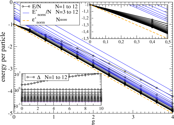
Figure 3: GS energies per particle as a function of $g$ for the model described by Eq. (21), “Modified Grover” ($N_{p}=N$). Here, $E^{\prime}_{\mathrm{norm}}/N=-1-g+3/N$ and $E/N$ is obtained by exact diagonalization. Upper Inset: particular of the plot in the range $g\in[0,0.5]$. Lower Inset: gap $\Delta$ as a function of ${g}$, for $N=1$ to $N=12$ (highest to lowest plot).

A.2 Fermions in a heterogeneous external field - Specularity with QPT

Let us consider $N_{\mathrm{p}}$ fermions in a 1D chain of $N\geq N_{\mathrm{p}}$ sites with open boundary conditions (OBCs) governed by a Hamiltonian which is a simple modification of Eq. (14), namely,

$$H=-\sum_{i=1}^{N-1}\left(c^{\dagger}_{i}c_{i+1}+c^{\dagger}_{i+1}c_{i}\right)-{g}N_{\mathrm{p}}c^{\dagger}_{1}c_{1}.$$ (26)

If $K$ and $V$ correspond to the first and second term of Eq. (26), respectively, we can analyze this model as done above by setting $N_{\mathrm{imp}}=1$ and replacing $g$ with $gN_{\mathrm{p}}$. In particular, from Eqs. (12) and (13) it now follows

$$M_{\mathrm{cond}}=\frac{N_{\mathrm{p}}}{N}M,\qquad M=\binom{N}{N_{\mathrm{p}}},$$ (27)

$$E_{\mathrm{cond}}/N_{\mathrm{p}}=\left\{\begin{array}[]{ll}E^{(0)}(N-1,N_{\mathrm{p}})/N_{\mathrm{p}},&\quad g<0\\ -g+E^{(0)}(N-1,N_{\mathrm{p}}-1)/N_{\mathrm{p}},&\quad g>0\end{array}\right.$$ (30)

$$E_{\mathrm{norm}}/N_{\mathrm{p}}=\left\{\begin{array}[]{ll}-g+E^{(0)}(N-1,N_{\mathrm{p}}-1)/N_{\mathrm{p}},&\quad g<0,\\ E^{(0)}(N-1,N_{\mathrm{p}})/N_{\mathrm{p}},&\quad g>0.\end{array}\right.$$ (33)

In Fig. 4 we show the analysis of this model for $g\in[-2,1]$ in the half-filling case $N_{\mathrm{p}}=N/2$. Despite the fact that $M_{\mathrm{cond}}=M/2$, we have $\epsilon=\min\{\epsilon_{\mathrm{cond}},\epsilon_{\mathrm{norm}}\}$. As in the previous case, this is explained by switching the role between $K$ and $V$, and observing that $M^{\prime}_{\mathrm{cond}}=1$. Note that now we have a first-order QPT that takes place at $g_{\mathrm{c}}=0$. Quite interestingly, in this QPT the gap $\Delta$ does not take any minimum in correspondence of the critical point, and, for given $N$, remains constant (see the discussion in the Introduction).

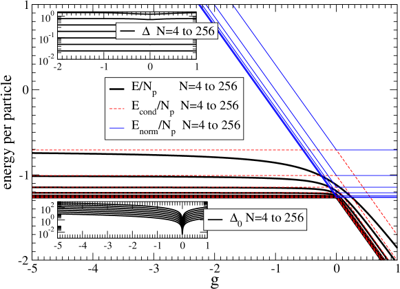
Figure 4: GS energies per particle as a function of ${g}$ for the model described by Eq. (26) (spinless fermions with an extensive non uniform external field) at half-filling. Here $E_{\mathrm{cond}}$ is given by Eq.(30) and $E$ is obtained by exact diagonalization. Upper Inset: gap $\Delta(N)$ for $N=4$ to $N=256$ (highest to lowest plot). Lower Inset: $\Delta_{1}$ as a function of ${g}$ for $N=4$ to $N=256$ (highest to lowest plot). It turns out that, at half-filling, the common discontinuity of $E_{\mathrm{cond}}$ and $E_{\mathrm{norm}}$ at $g=0$ gets exactly canceled (which explains why in the present case we have continuous plots).

A.3 Counter Example

From the previous examples, it turns out to be clear that, if we want to find a case where $\epsilon<\min\{\epsilon_{\mathrm{norm}},\epsilon_{\mathrm{cond}}\}$, as well as $\epsilon<\min\{\epsilon^{\prime}_{\mathrm{norm}},\epsilon^{\prime}_{\mathrm{cond}}\}$, we have to control that both $M_{\mathrm{cond}}/M\not\to 0$ and $M_{\mathrm{cond}}^{\prime}/M\not\to 0$. A very simple model where this occurs, is a system of $N$ spins in which only one of them is not free and is subject to an extensive external field and an extensive hopping:

$$H=-N|\uparrow^{x}\rangle\langle\uparrow^{x}|\bigotimes_{i=2}^{N}I_{i}-gN|\uparrow^{z}\rangle\langle\uparrow^{z}|\bigotimes_{i=2}^{N}I_{i}.$$ (34)

If we identify as $K$ and $V$ the first and second terms in Eq. (34), respectively, we have $V_{\mathrm{min}}=-gN$ and $\mathbb{F}_{\mathrm{cond}}=\mathrm{span}\{|\uparrow^{z}\rangle\otimes|u\rangle\}$, where $|u\rangle$ is an arbitrary state of $N-1$ spins. Therefore, in this case we have $M_{\mathrm{cond}}=M/2$ and

$$|E_{\mathrm{cond}}\rangle=|\uparrow^{z}\rangle\otimes|u\rangle,\quad E_{\mathrm{cond}}/N=-\frac{1}{2}-g,$$ (35)

$$|E_{\mathrm{norm}}\rangle=|\downarrow^{z}\rangle\otimes|v\rangle,\quad E_{\mathrm{norm}}/N=-\frac{1}{2},$$ (36)

where $|u\rangle$ and $|v\rangle$ are two arbitrary states of $N-1$ spins. On the other hand, if we define $K^{\prime}=V$ and $V^{\prime}=K$, we have $V^{\prime}_{\mathrm{min}}=-N$ and $\mathbb{F}^{\prime}_{\mathrm{cond}}=\mathrm{span}\{|\uparrow^{x}\rangle\otimes|u\rangle\}$, where $|u\rangle$ is an arbitrary state of $N-1$ spins. It follows that $M^{\prime}_{\mathrm{cond}}=M/2$ and

$$|E_{\mathrm{cond}}^{\prime}\rangle=|\uparrow^{x}\rangle\otimes|u\rangle,\quad E^{\prime}_{\mathrm{cond}}/N=-1-\frac{1}{2}g,$$ (37)

$$|E^{\prime}_{\mathrm{norm}}\rangle=|\downarrow^{x}\rangle\otimes|v\rangle,\quad E^{\prime}_{\mathrm{norm}}/N=-\frac{1}{2}g,$$ (38)

$|v\rangle$ being an arbitrary state of $N-1$ spins. Finally, we observe that the exact eigenvalues $E_{\pm}$ of the Hamiltonian (34) are easily calculated, the corresponding values per particle being

$$E_{\pm}/N=-\frac{1}{2}(1+g)\pm\frac{1}{2}\sqrt{1+g^{2}}.$$ (39)

We conclude that, as expected, the ground state energy per particle $E_{-}/N$ is, for any value of $g>0$, strictly smaller than any of the energies given in Eqs. (35)-(38), i.e., in the thermodynamic limit, $\epsilon<\min\{\epsilon_{\mathrm{norm}},\allowbreak\epsilon_{\mathrm{cond}},\allowbreak\epsilon^{\prime}_{\mathrm{norm}},\allowbreak\epsilon^{\prime}_{\mathrm{cond}}\}$.

A.4 Final remark

It would be interesting to analyze more intermediate situations in which $\min\{M_{\mathrm{cond}}/M,M^{\prime}_{\mathrm{cond}}/M\}$ goes to zero slowly in the thermodynamic limit, and to analyze how fast the error obtained by assuming $E/N_{\mathrm{p}}=\min\{E_{\mathrm{cond}}/N_{\mathrm{p}},\allowbreak E_{\mathrm{norm}}/N_{\mathrm{p}},\allowbreak E^{\prime}_{\mathrm{cond}}/N_{\mathrm{p}},\allowbreak E^{\prime}_{\mathrm{norm}}/N_{\mathrm{p}}\}$ goes to zero in such limit. This will be the subject of future works.

Appendix B Comparing OBC with PBC

Here, we elaborate on the model of Eq. (14) and compare the case with OBC, Fig. 5, with the case with PBC, Fig. 6. We observe that only marginal differences emerge and the critical point remains located in the same position of the OBC case, $g_{\mathrm{c}}\simeq 4$. In Section 4 we show a case with OBC to avoid the sign problem which affects the MCS of any fermionic system, except those in 1D with OBC. In our case, this would affect the MCS of $E_{\mathrm{norm}}$ (whereas $E$ and $E_{\mathrm{cond}}$ are evaluated via exact diagonalization and analytically) reported in support of the general theory, even tough, we actually locate the critical point by means of $\Delta_{1}$, which does not make use of $E_{\mathrm{norm}}$. Interestingly, as mentioned in Section 4, we observe that the gap $\Delta$ does not present a minimum in correspondence of $g_{\mathrm{c}}$. In fact, for $g\to 0$, the GS energy of the model with PBC becomes degenerate, causing a null gap in such a limit. However, as in all the other cases, $\Delta$ changes dramatically its character when passing from the normal phase, $g<g_{\mathrm{c}}$, where it has a wildly oscillating behavior, to the condensed phase, $g>g_{\mathrm{c}}$, where it has a clear smooth behavior.

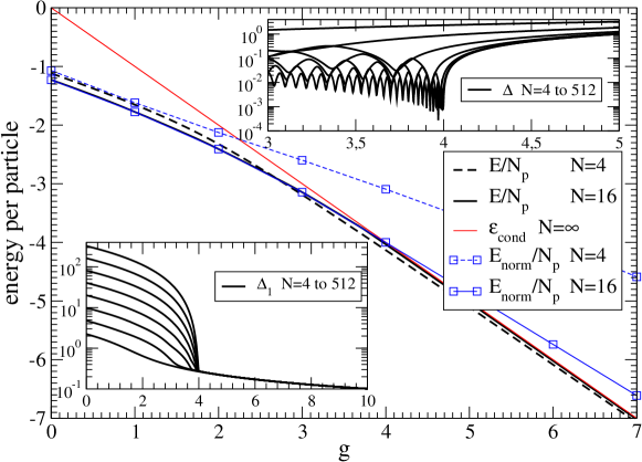
Figure 5: GS energies per particle as a function of $g$ for the model described by Eq. (14) (spinless fermions) with $N_{\mathrm{p}}=N_{\mathrm{imp}}=N/2$ in the case of OBC. Here, $\epsilon_{\mathrm{cond}}=-g$ and $E$ is obtained by exact diagonalization. Upper Inset: gap $\Delta$ as a function of $g$ around the critical point $g_{c}\simeq 4.0$, for $N=4$ to $N=512$ via powers of 2 (highest to lowest plot). Lowest Inset: the function $\Delta_{1}$, for $N=4$ to $N=512$ via powers of 2 (lowest to highest).

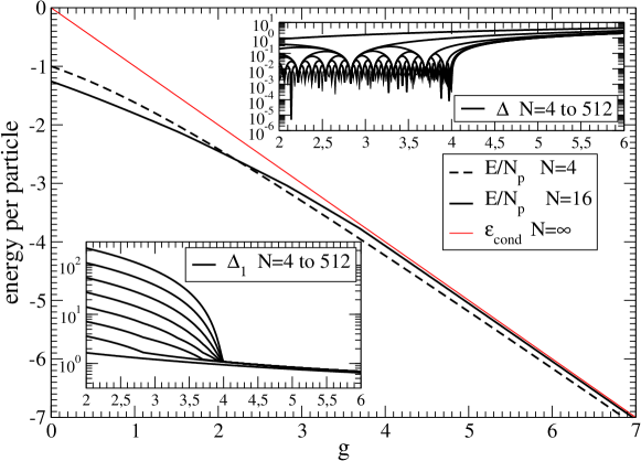
Figure 6: As in Fig. 5 for PBC.

Similar considerations hold in the case of spinless fermions with an attractive interaction, Eq. (17), compare Fig. 1c of Section 5 with Fig. 7.

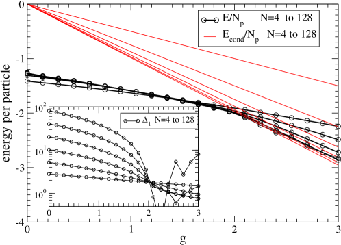
Figure 7: GS energies per particle as a function of $g$ for the model described by Eq. (17) (hard-core bosons) with $N_{\mathrm{p}}=N/2$ in the case of PBC. Here, $E_{\mathrm{cond}}/N_{\mathrm{p}}=-g(N_{\mathrm{p}}-1)/N_{\mathrm{p}}$ and $E$ is obtained by MCSs. Note that, at $g=0$, the lowest plot corresponds to the case $N=4$. Inset: the function $\Delta_{1}$, for $N=4$ to $N=128$ via powers of 2 (lowest to highest). As in the case of Fig. 1c, we see also here that the relation $E(N)/N_{\mathrm{p}}\leq E_{\mathrm{cond}}(N)/N_{\mathrm{p}}$ is often violated for large $N$ and $g>g_{\mathrm{c}}$ due to the large fluctuations occurring in the MCSs (see discussion in Sec. D).

Appendix C A further non trivial example with a second-order QPT

We have pointed out that our theory encoded in Eqs. (2) and (3), detects only first-order QPTs. At the same time, we have stressed that our Eq. (2), provided that $M_{\mathrm{cond}}/M\to 0$, is an identity that holds in any situation, regardless of any possible QPT and, in particular, regardless of the existence of a solution of Eq. (3). This fact has been made concrete by showing the analysis of the 1D Ising model in the presence of a transverse field, Eq. (16) and Fig. 1(d). To further support our claim, we now consider a generalization of the 1D Ising model that, besides the usual two-spin interaction, includes also a four-spin interaction as follows

$$H=-\sum_{i=1}^{N}\sigma_{i}^{x}-g\sum_{i=1}^{N}\sigma_{i}^{z}\sigma_{i+1}^{z}-g^{\prime}\sum_{i=1}^{N}\sigma_{i}^{z}\sigma_{i+1}^{z}\sigma_{i+2}^{z}\sigma_{i+3}^{z},\qquad N\geq 4,$$ (40)

where $g^{\prime}\geq 0$ is, besides $g$, a second free dimensionless parameter and PBC are understood. The aim of the present Appendix is threefold: by making use of extensive NDs, we demonstrate that: (i) Eq. (2) is satisfied, (ii) Eq. (3) has no finite solution, and (iii) the system undergoes a second-order QPT.

Case $g^{\prime}=0$. Before providing such demonstrations for the general Hamiltonian (40), it is useful to consider again the Ising case $g^{\prime}=0$. From Fig. 1(d) it is evident that, for any $g$, $E_{\mathrm{norm}}(N)/N\to\epsilon$ for $N\to\infty$. Since $M_{\mathrm{cond}}/M\to 0$, one may wonder that the result $\epsilon=\epsilon_{\mathrm{norm}}$ is a violation of Eq. (2). However, this is not the case, Eq. (2) holds true because we also have $\epsilon_{\mathrm{norm}}<\epsilon_{\mathrm{cond}}$ for any $g$. This inequality can be numerically validated as follows. At any finite size $N$, the curves $E_{\mathrm{norm}}(N)/N$ and $\epsilon_{\mathrm{cond}}$ cross, as a function of $g$, at the point $g_{\mathrm{cross}}(N)$, see Fig. 1(d). From Fig. 8, where we plot $g_{\mathrm{cross}}(N)$ as a function of $N$, it is evident that, after an initial transient, $g_{\mathrm{cross}}(N)$ grows linearly with $N$. The inequality $\epsilon_{\mathrm{norm}}<\epsilon_{\mathrm{cond}}$ for any $g$, allows also to conclude that Eq. (3) is not satisfied at any finite $g$. This excludes, therefore, the possibility of a first-order QPT. It is well known, however, that the Ising model has a second-order QPT at $g=1$. Whereas there exist several methods to show up the second-order nature of this QPT, in our framework, where we mainly work with the GS energy, it is convenient to analyze the nature of the possible singularities of $\epsilon(g)$ with respect to $g$. We remind that a QPT transition is classified of first-order when the GS energy per particle $\epsilon(g)$ has a jump discontinuity in its first derivative $\epsilon^{\prime}(g)=d\epsilon(g)/dg$, while it is classified of second-order when $\epsilon^{(k)}(g)=d^{k}\epsilon(g)/dg^{k}$ has a discontinuity for some $k\geq 2$. Such a definition parallels the definition of classical, finite temperature, QPT in terms of the thermodynamic limit of the free energy per particle. Figure 9 shows $\epsilon(g)$, $\epsilon^{\prime}(g)$ and $\epsilon^{\prime\prime}(g)$, where $\epsilon(g)$ is the exact GS energy per particle of the 1D Ising model ($g^{\prime}=0$) in the thermodynamic limit, as given by Eq. (20). Clearly, we are facing the well known scenario of a second-order QPT, where $\epsilon^{\prime}(g)$ is continuous, while $\epsilon^{\prime\prime}(g)$ has a singularity at the critical point $g_{c}=1$.

Figure 8: Plot of $g_{\mathrm{cross}}(N)$ versus $N$ for the 1D Ising model (corresponding to the choice $g^{\prime}=0$ in Eq. (40)) for $N=5,6,\ldots 22$. The crossing point $g_{\mathrm{cross}}(N)$ is defined as the value of $g$ at which $E_{\mathrm{norm}}(N)/N=\epsilon_{\mathrm{cond}}$, where $\epsilon_{\mathrm{cond}}=-g$ and $E_{\mathrm{norm}}(N)$ is evaluated by NDs.

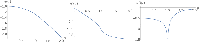
Figure 9: From left to right: plots of $\epsilon(g)$ , $\epsilon^{\prime}(g)$, and $\epsilon^{\prime\prime}(g)$ versus $g$, where $\epsilon(g)$ is the exact GS energy per particle of the 1D Ising model ($g^{\prime}=0$) in the thermodynamic limit, as given by Eq. (20).

Case $g^{\prime}>0$. For $g^{\prime}\neq 0$ the Hamiltonian (40) is rather non trivial. Nevertheless, in the ferromagnetic case $g^{\prime}>0$, the scenario obtained in the Ising case ($g^{\prime}=0$) remains essentially unchanged. For simplicity, we set $g^{\prime}=g$. The analysis for different positive values of $g^{\prime}$, not reported here, leads to the same qualitative behavior. In Figs. 10, 11, and 12, we see, respectively, the analogous of Figs. 1(d), 8, and 9 corresponding to the Ising case $g^{\prime}=0$. It is evident that, also for $g^{\prime}>0$, we have: (i) Eq. (2) is satisfied, (ii) Eq. (3) has no finite solution in terms of the parameter $g^{\prime}=g$, and (iii) the system undergoes a second-order QPT (in this case the critical point being located near $g=0.44$). It is worth to mention that the fact that the observed QPT of this 1D model remains of second-order for any non negative value of $g^{\prime}$, is quite different from the mean-field case where, at least classically, as is known, for suitable positive values of $g$ and $g^{\prime}$ one can have also first-order QPTs.

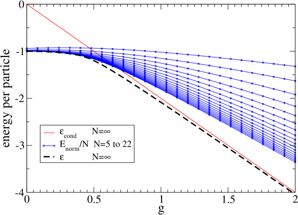
Figure 10: GS energies per particle for the model with Hamiltonian (40) in the case $g^{\prime}=g$: $\epsilon_{\mathrm{cond}}=-2g$ (continuous line), $\epsilon$ (dashed line), $E_{\mathrm{norm}}/N$ (line with points) for $N$= 5 to 22 (top to bottom). Here $\epsilon$ has been obtained by using $\epsilon\simeq E(N)/N$ for any $N$ large enough. In fact, as in the Ising case ($g^{\prime}=0$), also in this case $E(N)/N\to\epsilon$ very quickly, the differences between $N=12$ and $N=13$, for example, being unrecognizable at the shown scale. Here, we have evaluated $\epsilon\simeq E(N)/N$ with $N=22$.

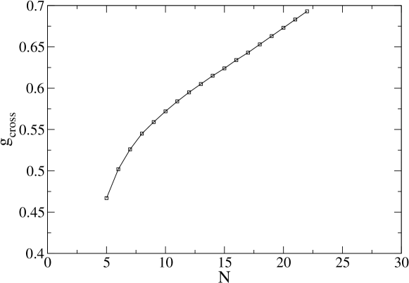
Figure 11: Plot of $g_{\mathrm{cross}}(N)$ versus $N$ for the model with Hamiltonian (40) in the case $g^{\prime}=g$ for $N=5,6,\ldots 22$. The crossing point $g_{\mathrm{cross}}(N)$ is defined as the value of $g$ at which $E_{\mathrm{norm}}(N)/N=\epsilon_{\mathrm{cond}}$, where $\epsilon_{\mathrm{cond}}=-2g$ and $E_{\mathrm{norm}}(N)$ is evaluated by NDs.

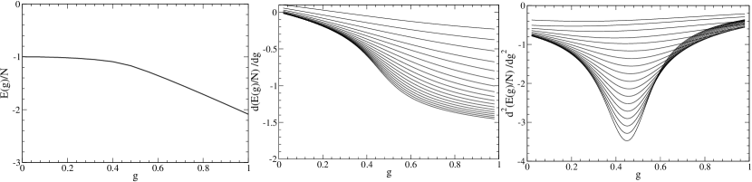
Figure 12: From left to right: plots of $E(g)/N$, $E^{\prime}(g)/N$, and $E^{\prime\prime}(g)/N$ as a function of $g$ for $N=5$ to 22 for the model with Hamiltonian (40) obtained by NDs. In the plot of $E(g)/N$ the curves obtained for different values of $N$ are indistinguishable.

Appendix D Monte Carlo simulations

The method used to perform our MCSs on lattice systems is based on an exact probabilistic representation of the quantum dynamics via Poisson processes that, virtually, reproduce the trajectories determined by the hopping operator $K$ [37, 38]. The corresponding Monte Carlo sampling is exact in the sense that there are no systematic errors due to any finite-time approximations (there is no Trotter approximation, see, e.g., [28]). The GS energy of a system governed by a Hamiltonian $H$ can then be obtained from the evaluations of the matrix elements of the evolution operator $\exp(-Ht)$ at imaginary times $t$ in the limit $t\to+\infty$. As in any MCS, sampling the matrix elements of $\exp(-Ht)$ involves fluctuations that increase exponentially with $t$. These fluctuations can be reduced by using a reconfiguration technique [39, 40]: instead of following many independent sample-trajectories that evolve during a long time $t$, one follows the evolution of a set of $\mathcal{M}\gg 1$ simultaneous trajectories that evolve along the shorter times $\Delta t=t/R$, where $R$ is an integer sufficiently large to keep the fluctuation along $\Delta t$ small. At the end of each time step $\Delta t$, the final configurations with index $i=1,\dots,\mathcal{M}$ are given a suitable weight $p_{i}$ which is used to generate randomly the initial configurations of the subsequent time step. The procedure stops after $R$ time steps. In the limit $\mathcal{M}\to\infty$ this procedure becomes exact (no bias is introduced) [38]. By a suitable choice of $\mathcal{M}$ and $R$ this technique allows us to handle the MCS of our models even close to the critical points, where in principle we should let $t\gg 1/\Delta$, where $\Delta$ is the gap of the model.

$N\leavevmode\nobreak\$	$N_{\mathrm{p}}\leavevmode\nobreak\$	$\Delta t\leavevmode\nobreak\$	$R\leavevmode\nobreak\$
4	2	16	64
8	4	16	128
16	8	16	256
32	16	32	512
64	32	32	1024

Table 1: Statistical parameters used for the MCSs of 1D free fermions in a non-uniform external field (Fig. 1b and Fig. 5).

$N\leavevmode\nobreak\$	$N_{\mathrm{p}}\leavevmode\nobreak\$	$\Delta t\leavevmode\nobreak\$	$R\leavevmode\nobreak\$
4	2	16	64
8	4	16	128
16	8	16	256
32	16	64	512
64	32	64	1024
128	64	64	2048

Table 2: Statistical parameters used for the MCSs of 1D interacting fermions and 1D hard-core bosons (Fig. 1c and Fig. 7).

The above procedure cannot be applied for $\Delta t$ too small: below a certain threshold of $\Delta t$, the system simply does not evolve. In fact, given the hopping operator $K$, one must take into account that the mean number of jumps $\left\langle N\right\rangle_{t}$ of a virtual trajectory along a time $t$ is, up to a dimensional factor that we set to 1 in our models, $\left\langle N\right\rangle_{t}=E^{(0)}t$, where $E^{(0)}$ is the GS energy of the system without potential, i.e., the case with $g=0$. Therefore, it is necessary to choose $R$ such that $\Delta tE^{(0)}\geq 1$. In the absence of a QPT the optimal choice corresponds to $\Delta t=1/E^{(0)}\propto 1/N_{\mathrm{p}}$ which, in the absence of any sign problem, allows to perform efficient simulations for systems of large size [38]. However, if the model undergoes a QPT, such a choice works only far from the critical point and larger values of $\Delta t$ must be considered. Given the magnitude of the desired maximal simulation times to be performed on an ordinary PC, ranging in our cases from a few ours to a few days, there is not a simple recipe to select the optimal values of $\mathcal{M}$ and $R$, the best criterion being empirical with the constrain $\Delta tE^{(0)}\geq 1$. In Tables I and II we show the statistical parameters chosen to perform our MCSs. In all cases we have used a single set of $\mathcal{M}=2^{20}$ parallel trajectories. Table I refers to Fig. 1b and Fig. 5. In these cases the MCSs have been used only for evaluating $E_{\mathrm{norm}}(N)$, which actually is not used to locate the critical point, but only to show (for a few system sizes $N$) how the general theory takes effect. Table II refers to the cases of Fig. 1c and Fig. 7. In all cases, as we approach the region $g\geq g_{\mathrm{c}}$ the statistics becomes more demanding, an issue which becomes more pronounced in the presence of interaction (see the fluctuations in the Inset of Fig. 1c and in the Fig. 7 for $g\geq g_{\mathrm{c}}$). Indeed, a sign of the fact that, for $g>g_{\mathrm{c}}$, the MCSs are affected by large fluctuations emerges by observing that the relation $E(N)\leq E_{\mathrm{cond}}(N)$ is often violated for large $N$ and $g>g_{\mathrm{c}}$. However, this problem does not prevent us to locate well the critical point $g_{\mathrm{c}}$ also in the presence of interaction. These large fluctuations could be reduced by exploiting the partial information that we have about the GS for $g>g_{\mathrm{c}}$ and using importance sampling, as explained in [38]. Such a refinement is however beyond the aim of the present work.

References

References

- [1] P. W. Anderson, Infrared Catastrophe in a Fermi Gas with local scattering potentials, Phys. Rev. Lett. 18, 1049 (1967).
- [2] S. L. Sondhi, S. M. Girvin, J. P. Carini, and D. Shahar Continuous quantum phase transitions Rev. Mod. Phys. 69, 315 (1997).
- [3] S. Sachdev, Quantum Phase Transitions, Sec. Ed., Cambridge University Press (2011).
- [4] M. Vojta, Quantum Phase Transitions, Rep. Prog. Phys. 66, 2069 (2003).
- [5] A. Dutta, G. Aeppli, B. K. Chakrabarti, U. Divakaran, T. F. Rosenbaum, D. Sen, Quantum Phase Transitions in Transverse Field Models, Cambridge University Press (2015).
- [6] L. D. Landau and E. M. Lifshitz (1981), Quantum Mechanics, Pergamon Press (1981).
- [7] M. Suzuki, Relationship between d-Dimensional Quanta! Spin Systems and (d+ I) -Dimensional Ising Systems , Progr. Th. Phys, 56, 1454 (1976).
- [8] C. Pfleiderer, Why first order quantum phase transitions are important, J. Phys.: Condens. Matter 17, S987 (2005).
- [9] M. A. Continentino, A. S. Ferreira, First-order quantum phase transitions, J. Magnetism and Magnetic Materials 310, 828 (2007).
- [10] M. Campostrini, J. Nespolo, A. Pelissetto, and E. Vicari, Finite-Size Scaling at First-Order Quantum Transitions Phys. Rev. Lett. 113, 070402 (2014).
- [11] M. Campostrini, J. Nespolo, A. Pelissetto, and E. Vicari, Finite-size scaling at the first-order quantum transitions of quantum Potts chains Phys. Rev. E 91, 052103 (2015).
- [12] I. Bose and E. Chattopadhyay, Macrosopic entanglement jumps in model spin systems, Phys. Rev. A 66, 062320 (2002).
- [13] J. Vidal, R. Mosseri, and J. Dukelsky, Entanglement in a first order quantum phase transition, Phys. Rev. A 69, 054101 (2004).
- [14] M. Ostilli and C. Presilla, The exact ground state for a class of matrix Hamiltonian models: quantum phase transition and universality in the thermodynamic limit J. Stat. Mech. (2006) P11012 (2006).
- [15] T. Jorg, F. Krzakala, J. Kurchan, and A. C. Maggs, Simple Glass Models and their Quantum Annealing, Phys. Rev. Lett. 101, 147204 (2008).
- [16] T. Jorg, F. Krzakala, J. Kurchan, A. C. Maggs, and J. Pujos, Energy gaps in quantum first-order mean-field–like transitions: The problems that quantum annealing cannot solve, Europhys. Lett. 89, 40004 (2010).
- [17] J. Tsuda, Y. Yamanaka, H. Nishimori, Energy gap at first-order quantum phase transitions: An anomalous case, J. Phys. Soc. Jpn. 82, 114004 (2013).
- [18] M. Ezawa, Y. Tanaka and N. Nagaosa, Topological Phase Transition without Gap Closing, Sci. Rep. 3, 2790 (2013).
- [19] S. Rachel, Quantum phase transitions of topological insulators without gap closing, J. Phys.: Condens. Matter 28, 405502 (2016).
- [20] A. Amaricci, J. C. Budich, M. Capone, B. Trauzettel, G. Sangiovanni, First order character and observable signatures of topological quantum phase transitions, Phys. Rev. Lett. 114, 185701 (2015).
- [21] B. Roy, P. Goswami, J. D. Sau, Continuous and discontinuous topological quantum phase transitions, Phys. Rev. B 94, 041101(R) (2016).
- [22] S.-J. Gu, Int. J. Mod. Phys. B 24, 4371 (2010).
- [23] Dependencies from the Hamiltonian parameters and from are often left understood.
- [24] M. Ostilli, Quantum Phase Transitions induced by Infinite Dilution in the Fock Space: a General Mechanism. Proof and discussion, arXiv:0905.4496 (2009).
- [25] M. Ostilli and C. Presilla, Exact Monte Carlo time dynamics in many-body lattice quantum systems, J. Phys. A 38, 405 (2005).
- [26] L. K. Grover: A fast quantum mechanical algorithm for database search, arXiv:quant-ph/9605043.
- [27] C. H. Bennett, E. Bernstein, G. Brassard, U. Vazirani, The strengths and weaknesses of quantum computation, SIAM Journal on Computing, 26 1510 (1997).
- [28] D. M. Ceperley and M. H. Kalos, Monte Carlo Methods in Statistical Physics, ed. K. Binder (Heidelberg: Springer) (1992).
- [29] V. Bapst, L. Foini, F. Krzakala, G. Semerjian, F. Zamponi, The quantum adiabatic algorithm applied to random optimization problems: The quantum spin glass perspective, Phys. Rep. 523, 127 (2013).
- [30] E. Y. Loh, J. E. Gubernatis, R. T. Scalettar, S. R. White, D. J. Scalapino,R. L. Sugar, Sign problem in the numerical simulation of many-electron systems, Phys. Rev. B 41, 9301 (1990).
- [31] E. Lieb, T. Schultz, and D. Mattis, Two soluble models of an antiferromagnetic chain, Annals of Phys., 16, 407 (1961).
- [32] S. Suzuki, Jun-ichi Inoue, and B. K. Chakrabarti, Quantum Ising Phases and Transitions in Transverse Ising Models, (Lecture Notes in Physics), Springer, (2012).
- [33] R. J. Baxter, One-dimensional anisotropic Heisenberg chain, Ann. Phys. (N.Y.) 70, 323 (1972).
- [34] I. Affleck, Field Theory Methods and Quantum Critical Phenomena, in Les Houches, Session XLIX, 588 (1988).
- [35] P. Pfeuty, The one-dimensional Ising model with a transverse field, Ann. Phys. (N.Y.) 57, 79 (1970).
- [36] M. Ostilli and C. Presilla, Wigner crystallization of electrons in a one-dimensional lattice: a condensation in the space of states, arXiv:1912.11357.
- [37] M. Beccaria, C. Presilla, G. F. De Angelis, and G. Jona Lasinio, An exact representation of the fermion dynamics in terms of Poisson processes and its connection with Monte Carlo algorithms , Europhys. Lett. 48 243 (1999).
- [38] M. Ostilli and C. Presilla, Exact Monte Carlo time dynamics in many-body lattice quantum systems, J. Phys. A: Math. Gen. 38, 405 (2005).
- [39] J H. Hetherington, Observations on the statistical iteration of matrices, Phys. Rev. A 30, 2713 (1984).
- [40] M. Calandra Buonaura and S. Sorella, Numerical study of the two-dimensional Heisenberg model using a Green function Monte Carlo technique with a fixed number of walkers, Phys. Rev. B 57, 11446 (1998).