General one-loop formulas for decay $h\rightarrow Z\gamma$

Abstract

Radiative corrections to the decay $h\rightarrow Z\gamma$ are evaluated in the one-loop approximation. The unitary gauge is used. The analytic result is expressed in terms of the Passarino-Veltman functions. The calculations are applicable for the Standard Model as well for a wide class of its gauge extensions. In particular, the decay width of a charged Higgs boson $H^{\pm}\rightarrow W^{\pm}\gamma$ can be derived. The consistence of our formulas and several specific earlier results is shown.

I Introduction

After the discovery of the Higgs boson particle at LHC in 2012 Htn ; Htn1 , many improved measurements confirmed the consistence of its quantum numbers and couplings with the Standard Model (SM) predictions, including the loop-induced coupling $h\gamma\gamma$ Khachatryan:2016vau ; HiggsExconstrain1 . Meanwhile, another loop-induced coupling $hZ\gamma$ related to the decay $h\rightarrow Z\gamma$ has not been measured yet even so that the predicted decay rate is of the same order as the one of $h\rightarrow\gamma\gamma$ in the SM case hzgapredict . The partial decay width $h\rightarrow Z\gamma$ was calculated within the SM framework and its supersymmetric extension hzga1 ; hzga2 ; Bardin:1991dp ; hzgamssm ; HHunter ; Cao:2013ur ; Belanger:2014roa ; Hammad:2015eca . From the experimental side, this decay channel is now been searched at the LHC by both CMS and ATLAS collaborations hzgaex1 ; hzgaex2 ; hzgaex3 . Many discussions concerning studies of this channel are going also in planned experimental projects as at the LHC as well as at future $e^{+}e^{-}$ and even 100 TeV proton-proton colliders hzgaexim1 ; hzgaexim2 . While the effective coupling $h\gamma\gamma$ is now very strictly constrained experimentally, the coupling $hZ\gamma$ might be still significantly different from the SM prediction in certain SM extensions because of the $Z$ boson couplings with new particles. Studies the decay of the SM-like Higgs boson $h\rightarrow Z\gamma$ affected by the presence of new fermions and charged scalars were performed in several models beyond the SM (BSM) having the same SM gauge group hzgamssm ; HzgaTHD ; GMmodel ; hdcay1 ; Dev:2013ff .

At the one loop level, the amplitude of the decay $h\rightarrow Z\gamma$ contains also contributions from new gauge boson loops of the BSM models constructed from larger electroweak gauge groups such as the left-right (LR), 3-3-1, and 3-4-1 models lr1 ; lr2 ; lr3 ; lr4 ; lr5 ; lr6 ; g331 ; g331a ; g331b ; g331c ; g331d ; g331e ; g331f ; g331g ; g341 ; g341a . Calculating these contributions is rather difficult in the usual ’t Hooft-Feynman gauge, because of the appearance of many unphysical states, namely Goldstone bosons and ghosts which always exist along with the gauge bosons. They create a very large number of Feynman diagrams. In addition, their couplings are indeed model dependent, therefore it is hard to construct general formulas determining vector loop contributions using the t’ Hooft-Feynman gauge. This problem has been mentioned recently GMmodel in a discussion of the Georgi-Machacek model, where only new Higgs multiplets are added to the SM. The reason is that the new Higgs bosons will change the couplings of unphysical states with the gauge bosons $Z$ and $W^{\pm}$. In the left-right models predicting new gauge bosons that contribute to the amplitude of the decay $h\rightarrow Z\gamma$, previous calculations in this gauge were also model dependent hzgalr1 ; hzgalr2 . An approach introduced recently in Ref. Goodsell:2017pdq for calculating the decay $h\rightarrow Z\gamma$, with the help of numerical computation packages, may be more convenient.

The technical difficulties caused by unphysical states will vanish if calculations have been done in the unitary gauge. There the number of Feynman diagrams as well as the number of necessary couplings become minimum, namely only those which contain physical states are needed. Then the Lorentz structures of these couplings are well defined, and hence the general analytic formulas of one-loop contributions from gauge boson loops can be constructed. But in the unitary gauge we face complicated forms of the gauge boson propagators, which generate many dangerous divergent terms. Fortunately, many of them are excluded by the condition of on-shell photon in the decay $h\rightarrow Z\gamma$. The remaining ones will vanish systematically when loop integrals are written in terms of the Passarino-Veltman (PV) functions PVfunc . This situation will be demonstrated in this work explicitly. Moreover, the choice of the unitary gauge allows us to derive general analytic formulas for one-loop contributions involving various gauge bosons to the amplitude of the decay $h\rightarrow Z\gamma$. The formulas will be given in terms of standard PV functions defined by ref. PVDenner and in the LoopTools library LoopTools . The analytic forms of these PV functions are also presented so that our results can be compared with the earlier results calculated independently in specific cases. In addition, the analytic formulas can be implemented into numerical stand-alone packages without dependence on the LoopTools. Our results can be translated into the general analytic form used to calculate the amplitudes of the charged Higgs decay $H^{\pm}\rightarrow W^{\pm}\gamma$ which is also an interesting channel predicted in many BSM models. Our results can be easily compared also with those given recently in GMmodel , which were calculated in the ’t Hooft-Feynman gauge. Moreover, our results can be cross-checked with another one-loop formula expressing new gauge boson contributions in the gauge-Higgs unification (GHU) model hzgaGHU .

The decay $H\rightarrow Z\gamma$ of the new heavy neutral Higgs boson $H$ in the SM supersymmetric model was also mentioned in Belanger:2014roa . The signal strength of this decay was shown to be very sensitive with the parameters of the model, hence it may give interesting information on the parameters once it is detected. Many other BSM also contain heavy neutral Higgs bosons $H$, and the one loop amplitudes of their decays $H\rightarrow Z\gamma$ may include many significant contributions that do not appear in the case of the SM-like Higgs boson. Some of the complicated contributions are usually ignored by qualitative estimations. The analytic formulas introduced in this work are enough to determine more quantitatively these approximations.

Apart from the above BSM with non-Abelian gauge group extensions, there are BSM with additional Abelian gauge groups Holdom:1985ag ; Babu:1996vt . These models predict new kinetic mixing parameters between Abelian gauge bosons, which appear in the couplings of the neutral physical gauge bosons including the SM-like one, for example see Cassel:2009pu . Our calculation in the unitary gauge are also applicable with only condition that couplings of physical states are determined.

Our paper is organized as follows. Section II will give the general notations and Feynman rules necessary for calculation of the width of the decay $h\rightarrow Z\gamma$ in the unitary gauge. In section III we present important steps of the derivation of the analytic formula for the total contribution of gauge boson loops. We also introduce all other one-loop contributions from possible new scalars and fermions appearing in BSM models. In section IV, the comparison between our results with previous ones will be discussed, including the case of charged Higgs decays. We will emphasize the contributions from gauge boson loops both in decays of neutral CP-even and charged Higgs bosons. Our result will be applied to discuss on two particular models in section V. In Conclusions we will highlight important points obtained in this work. In the first Appendix, we review notations of the PV functions given by LoopTools and their analytic forms used in other popular numerical packages. Two other Appendices contain detailed calculations of the one-loop fermion contributions to the amplitude $h\to Z\gamma$ and the relevant couplings in the LR models discussed in our work.

II Feynman diagrams and rules

The amplitude of the decay $h\rightarrow Z\gamma$ is generally defined as

$$\mathcal{M}(h\rightarrow Z\gamma) \equiv\mathcal{M}\left(Z_{\mu}(p_{1}),\gamma_{\nu}(p_{2}),h(p_{3})\right)\varepsilon^{\mu*}_{1}(p_{1})\varepsilon^{\nu*}_{2}(p_{2})$$

$$\equiv\mathcal{M}_{\mu\nu}\varepsilon^{\mu*}_{1}\varepsilon^{\nu*}_{2},$$ (1)

where $\varepsilon^{\mu}_{1}$ and $\varepsilon^{\nu}_{2}$ are the polarization vectors of the $Z$ boson and the photon $\gamma$, respectively. The external momenta $p_{1}$, $p_{2}$, and $p_{3}$ satisfy the condition $p_{3}=p_{1}+p_{2}$ with the directions denoted in figure 1 where one-loop Feynman diagrams contributing to the decay are presented. Only diagrams which are relevant in the unitary gauge are mentioned. The on-shell conditions are $p_{1}^{2}=m_{Z}^{2}$, $p_{2}^{2}=0$, and $p_{3}^{2}=m_{h}^{2}$.

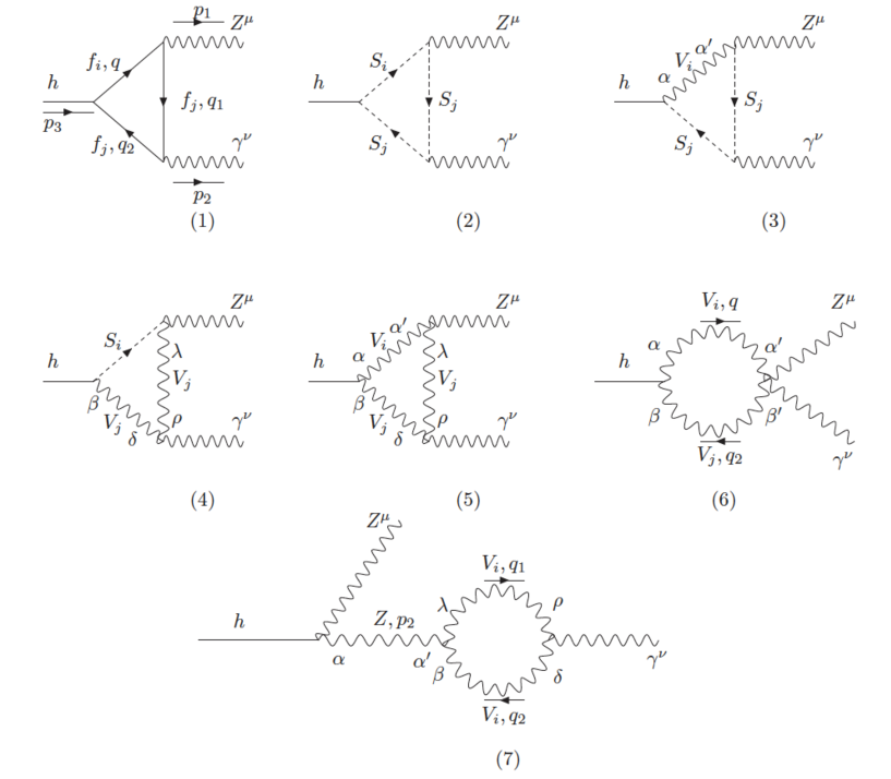
Figure 1: One-loop diagrams contributing to the decay $h\rightarrow Z\gamma$, where $f_{i,j}$, $S_{i,j}$ and $V_{i,j}$ are fermions, Higgs, and gauge bosons, respectively.

The decay amplitude is generally written in the following form hzgamssm :

$$\mathcal{M}_{\mu\nu}\equiv F_{00}\,g_{\mu\nu}+\sum_{i,j=1}^{2}F_{ij}p_{i\mu}p_{j\nu}+F_{5}\times i\epsilon_{\mu\nu\alpha\beta}p_{1}^{\alpha}p_{2}^{\beta},$$ (2)

where $\epsilon_{\mu\nu\alpha\beta}$ is the totally antisymmetric tensor with $\epsilon_{0123}=-1$ and $\epsilon^{0123}=+1$ peskin .

The equality $\varepsilon^{\nu*}_{2}p_{2\nu}=0$ for the external photon implies that $F_{12,22}$ do not contribute to the total amplitude (1). In addition, the $\mathcal{M}_{\mu\nu}$ in eq. (2) satisfies the Ward identity, $p_{2}^{\nu}\mathcal{M}_{\mu\nu}=0$, resulting in $F_{11}=0$ and hzgamssm

$$F_{00}=-(p_{1}.p_{2})F_{21}=\frac{(m_{Z}^{2}-m_{h}^{2})}{2}F_{21}.$$ (3)

Hence the amplitude (1) can be calculated through the form (2) via the following relations

$$\mathcal{M}(h\rightarrow Z\gamma) =\mathcal{M}_{\mu\nu}\varepsilon^{\mu*}_{1}\varepsilon^{\nu*}_{2},$$

$$\mathcal{M}_{\mu\nu} =F_{21}\left[-(p_{2}.p_{1})g_{\mu\nu}+p_{2\mu}p_{1\nu}\right]+F_{5}\times i\epsilon_{\mu\nu\alpha\beta}p_{1}^{\alpha}p_{2}^{\beta}.$$ (4)

The partial decay width then can be presented in the form HHunter ; GMmodel

$$\Gamma(h\rightarrow Z\gamma)=\frac{m_{h}^{3}}{32\pi}\times\left(1-\frac{m_{Z}^{2}}{m_{h}^{2}}\right)^{3}\left(|F_{21}|^{2}+|F_{5}|^{2}\right).$$ (5)

The above formula shows us that we need to find only two scalar coefficients $F_{21}$ and $F_{5}$ in eq. (4). Because $F_{5}$ arises from only chiral fermion loops, it is enough to pay attention to terms proportional to $F_{21}p_{2\mu}p_{1\nu}$ for gauge boson loops. Therefore calculations will be simplified, especially in the unitary gauge. Combining with notations of the PV functions PVfunc , we will determine explicitly which terms give contributions to $F_{21}p_{2\mu}p_{1\nu}$, and hence exclude step by step irrelevant terms throughout our calculations.

Calculation of the factor $F_{21}$ is very interesting because it does not receive contributions from diagrams which contain counterterm vertices. The Lorentz structures of the counterterm vertices are shown in figure 2.

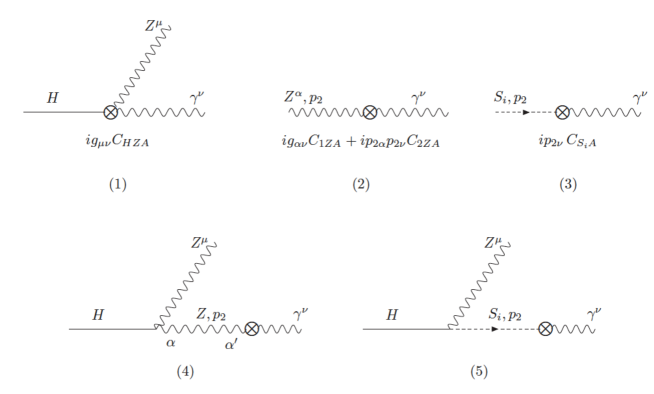
Figure 2: Counterterm vertices and related one-loop diagrams contributing to the one-loop amplitude of the decay $h\rightarrow Z\gamma$.

The first line represents three additional counterterm vertices. The second line shows two more diagrams. The total amplitude is the sum of three diagrams 1, 4, and 5 in figure 2 and all diagrams shown in figure 1. We can see in figure 2 that, the first diagram contributes only to $F_{00}$. In the unitary gauge, the propagator of a gauge boson is

$$\Delta^{\mu\nu}(k^{2},m^{2})=\frac{-i}{k^{2}-m^{2}}\left(g^{\mu\nu}-\frac{k^{\mu}k^{\nu}}{m^{2}}\right).$$ (6)

The Lorentz structures of the two remaining counterterms are

$$i\mathcal{M}^{\mathrm{CT}}_{(4)\mu\nu} \sim g_{\mu\alpha}\times\left(g^{\alpha\alpha^{\prime}}-\frac{p_{2}^{\alpha}p_{2}^{\alpha^{\prime}}}{m_{Z}^{2}}\right)\times\left(g_{\alpha^{\prime}\nu}C_{1ZA}+p_{2\alpha^{\prime}}p_{2\nu}C_{2ZA}\right)$$

$$=g_{\mu\nu}C_{1ZA}+p_{2\mu}p_{2\nu}\left(C_{2ZA}-\frac{C_{1ZA}}{m_{Z}^{2}}\right),$$

$$i\mathcal{M}^{\mathrm{CT}}_{(5)\mu\nu} \sim(p_{3}+p_{2})_{\mu}\times\left(p_{2\nu}C_{S_{i}A}\right)=(p_{1}+2p_{2})_{\mu}p_{2\nu}C_{S_{i}A},$$

which contribute only to $F_{00}$, $F_{12}$, and $F_{22}$. The result for the Lorentz structures is unchanged if the virtual gauge boson $Z$ in diagram 4 is replaced with the new ones in a gauge extended versions of the SM. As the result, $F_{21}$ is not affected by counterterms, therefore we do not need to include them in our calculation. In addition, $F_{21}$ is finite without including the related counterterm diagrams. A similar situation in two Higgs doublet models was discussed in HzgaTHD . Examples for Lorentz structures of the counterterms were given also, e.g., in refs. PVDenner ; grace .

Vertex	Coupling
$h\overline{f_{i}}f_{j}$	$-i\left(Y_{hf_{ij}L}P_{L}+Y_{hf_{ij}R}P_{R}\right)$
$hS^{Q}_{i}S^{-Q}_{j}$, $hS^{-Q}_{i}S^{Q}_{j}$	$-i\lambda_{hS_{ij}}$, $-i\lambda^{*}_{hS_{ij}}$
$h(p_{0})S^{-Q}_{i}(p_{-})V^{Q\mu}_{j}$, $h(p_{0})S^{Q}_{i}(p_{+})V^{-Q\mu}_{j}$	$ig_{hS_{i}V_{j}}(p_{0}-p_{-})_{\mu}$, $-ig^{*}_{hS_{i}V_{j}}(p_{0}-p_{+})_{\mu}$
$hV^{-Q\mu}_{i}V^{Q\nu}_{j}$, $hZ^{\mu}Z^{\nu}$	$ig_{hV_{ij}}g_{\mu\nu}$, $ig_{hZZ}g_{\mu\nu}$
$A^{\mu}\overline{f_{i}}f_{i}$, $A^{\mu}S^{Q}_{i}S^{-Q}_{i}$	$ie\,Q\gamma_{\mu}$, $ie\,Q(p_{+}-p_{-})_{\mu}$
$A^{\mu}(p_{0})V^{Q\nu}_{i}(p_{+})V^{-Q\lambda}_{i}(p_{-})$	$-ieQ\Gamma_{\mu\nu\lambda}(p_{0},p_{+},p_{-})$
$Z^{\mu}\overline{f_{i}}f_{j}$	$i\left(g_{Zf_{ij}L}\gamma_{\mu}P_{L}+g_{Zf_{ij}R}\gamma_{\mu}P_{R}\right)$
$Z^{\mu}S^{Q}_{i}(p_{+})S^{-Q}_{j}(p_{-})$	$ig_{ZS_{ij}}(p_{+}-p_{-})_{\mu}$
$Z^{\mu}V^{Q\nu}_{i}S^{-Q}_{j}$, $Z^{\mu}V^{-Q\nu}_{i}S^{Q}_{j}$	$ig_{ZV_{i}S_{j}}\,g_{\mu\nu}$, $ig^{*}_{ZV_{i}S_{j}}\,g_{\mu\nu}$
$Z^{\mu}(p_{0})V^{Q\nu}_{i}(p_{+})V^{-Q\lambda}_{j}(p_{-})$	$-ig_{ZV_{ij}}\Gamma_{\mu\nu\lambda}(p_{0},p_{+},p_{-})$
$Z^{\mu}A^{\nu}V^{Q\alpha}_{i}V^{-Q\beta}_{j}$	$-ie\,Q\,g_{ZV_{ij}}\left(2g_{\mu\nu}g_{\alpha\beta}-g_{\mu\alpha}g_{\nu\beta}-g_{\mu\beta}g_{\nu\alpha}\right)$

Table 1: Couplings involving the decay of CP even neutral Higgs $h\rightarrow Z\gamma$, in the unitary gauge. A new notation is $\Gamma_{\mu\nu\lambda}(p_{0},p_{+},p_{-})\equiv(p_{0}-p_{+})_{\lambda}g_{\mu\nu}+(p_{+}-p_{-})_{\mu}g_{\nu\lambda}+(p_{-}-p_{0})_{\nu}g_{\lambda\mu}$, where all momenta are incoming, and $p_{0,\pm}$ are respective momenta of $h$ and charged gauge and Higgs bosons with electric charges $\pm Q$, denoted as $V_{i,j}^{\pm Q}$ and $S_{i,j}^{\pm Q}$, respectively. The general case of four-gauge-boson coupling is $(2,-1,-1)\rightarrow(a_{1},a_{2},a_{3})$ and $g_{Z\gamma V_{ij}}\neq e\,Q\,g_{ZV_{ij}}$.

The Feynman rules used in our calculations are listed in table 1. We found them to appear commonly in many gauge extensions of the SM, for example in the models constructed from the following electroweak gauge symmetries: $SU(2)_{1}\times SU(2)_{2}\times U(1)_{Y}$, $SU(2)_{L}\times SU(2)_{R}\times U(1)_{Y}$, and $SU(3)_{L}\times U(1)_{X}$ gaugExtent221 ; Roitgrund:2014zka ; gaugExtent221b ; gaugExtent331 ; gaugExtent331a ; C0f , where an important relation $g_{Z\gamma V_{ij}}=e\,Q\,g_{ZV_{ij}}$ is valid. It results in that many complicated terms containing dangerous divergences in two contributions from diagrams 5 and 6 in figure 1 cancel each other out.

Following LoopTools LoopTools , figure 1 defines three internal momenta $q,q_{1},q_{2}$ as follows

$$q_{1}=q+k_{1}=q-p_{1},\quad q_{2}=q+k_{2}=q-(p_{1}+p_{2}),\quad p_{1}=-k_{1},\quad p_{2}=k_{1}-k_{2}.$$ (7)

Our formulas will be written in terms of common well-defined PV functions. Moreover, we can compare our results with previous works, as well as we can perform numerical estimates with the help of the LoopTools library. Definitions and notations for the PV functions are shown in Appendix A.

As the result, we only need to calculate the coefficient $F_{21}$. In the next section, we will present important steps of how to get contributions from pure gauge boson loops to $F_{21}$.

III Analytic formulas

III.1 Total contribution from diagrams with pure gauge boson mediations

Here we will consider calculation of the contribution from pure gauge boson loops to the decay amplitude of $h\rightarrow Z\gamma$. All of them were performed using the FORM language form1 ; form2 . Other contributions from diagrams which contain only one or two internal gauge boson lines are computed more easily.

The contribution from diagram 5 from figure 1 reads

$$i\mathcal{M}_{(5)\mu\nu} =2\times\int\frac{d^{d}q}{(2\pi)^{d}}(ig_{hV_{ij}}\,g_{\alpha\beta})\frac{-i}{D_{0}}\left(g^{\alpha\alpha^{\prime}}-\frac{q^{\alpha}q^{\alpha^{\prime}}}{m_{1}^{2}}\right)\times\left[-ig_{ZV_{ij}}\Gamma_{\mu\alpha^{\prime}\lambda}(-p_{1},q,-q_{1})\right]$$

$$\times\frac{-i}{D_{1}}\left(g^{\lambda\rho}-\frac{q_{1}^{\lambda}q_{1}^{\rho}}{m_{2}^{2}}\right)\times\left[-ie\,Q\,\Gamma_{\nu\rho\delta}(-p_{2},q_{1},-q_{2})\right]\times\frac{-i}{D_{2}}\left(g^{\delta\beta}-\frac{q_{2}^{\delta}q_{2}^{\beta}}{m_{2}^{2}}\right)$$

$$=2e\,Q\,g_{hV_{ij}}\,g_{ZV_{ij}}\int\frac{d^{d}q}{(2\pi)^{d}}\frac{1}{D_{0}D_{1}D_{2}}V_{1\mu\beta\lambda}V_{2\nu}^{\beta\lambda},$$ (8)

where $m_{1,2}\equiv m_{V_{i,j}}$, $D_{0}=q^{2}-m_{1}^{2}$, $D_{1,2}=q^{2}_{1,2}-m_{2}^{2}$,

$$V_{1\mu\beta\lambda} =g_{\alpha\beta}\left(g^{\alpha\alpha^{\prime}}-\frac{q^{\alpha}q^{\alpha^{\prime}}}{m_{1}^{2}}\right)\Gamma_{\mu\alpha^{\prime}\lambda}(-p_{1},q,-q_{1}),$$

$$V_{2\mu}^{\beta\lambda} =\left(g^{\lambda\rho}-\frac{q_{1}^{\lambda}q_{1}^{\rho}}{m_{2}^{2}}\right)\times\left[\Gamma_{\nu\rho\delta}(-p_{2},q_{1},-q_{2})\right]\left(g^{\delta\beta}-\frac{q_{2}^{\delta}q_{2}^{\beta}}{m_{2}^{2}}\right).$$ (9)

We note that factor 2 appearing in the first line of eq. (III.1) was added in order to count two different diagrams with opposite internal lines in the loops. It can be done because coupling constants $g_{hV_{ij}}$ and $g_{ZV_{ij}}$ are real numbers in all models that we consider here. Based on the structure of the PV functions, we know that $F_{21}p_{2\mu}p_{1\nu}$ gets contributions from parts having the following factors: $q_{\mu}q_{\nu}$, $q_{\mu}p_{1\nu}$, $p_{2\mu}q_{\nu}$, and $p_{2\mu}p_{1\nu}$. This means that we can do the following replacements in the calculation:

$$q_{1\mu} \rightarrow q_{\mu},\quad q_{2\mu}\rightarrow q_{\mu}-p_{2\mu},\quad q_{2\nu}\rightarrow q_{\nu}-p_{1\nu}=q_{1\nu},$$

$$k_{1\mu} \rightarrow 0,\quad k_{2\mu}\rightarrow-p_{2\mu},\quad k_{1\nu},\,k_{2\nu}\rightarrow-p_{1\nu},\quad g_{\mu\nu}\rightarrow 0.$$ (10)

After some intermediate steps shown in Appendix B, and combining with the relations $q^{2}=D_{0}+m_{1}^{2}$ and $D_{1,2}=q_{1,2}^{2}+m^{2}_{2}$, we have

$$i\mathcal{M}_{(5)\mu\nu} \rightarrow\left[e\,Q\,g_{hV_{ij}}\,g_{ZV_{ij}}\right]\times\int\frac{d^{d}q}{(2\pi)^{d}}\times\frac{1}{m_{1}^{2}m_{2}^{2}}$$

$$\times\left\{q_{\mu}q_{\nu}\left[-\frac{1}{D_{2}}-\frac{1}{D_{0}}+\frac{2(m_{1}^{2}-m_{2}^{2}+m_{Z}^{2})}{D_{1}D_{2}}+\frac{m_{1}^{2}+m_{2}^{2}+m_{h}^{2})}{D_{0}D_{2}}\right.\right.$$

$$\left.\left.+\frac{8(d-2)m_{1}^{2}m_{2}^{2}+2\left(m_{1}^{2}+m_{2}^{2}+m_{h}^{2}\right)(m_{1}^{2}+m_{2}^{2}-m_{Z}^{2})}{D_{0}D_{1}D_{2}}\right]\right.$$

$$+\left.q_{\mu}p_{1\nu}\left[\frac{1}{D_{2}}+\frac{1}{D_{0}}-\frac{2(m_{1}^{2}-m_{2}^{2}+m_{Z}^{2})}{D_{1}D_{2}}-\frac{5m_{1}^{2}+3m_{2}^{2}+m_{h}^{2}}{D_{0}D_{2}}\right.\right.$$

$$\left.\left.+\frac{2(m_{1}^{2}+m_{2}^{2}-m_{Z}^{2})}{D_{0}D_{1}}-\frac{8(d-2)m_{1}^{2}m_{2}^{2}+2\left(m_{1}^{2}+m_{2}^{2}+m_{h}^{2}\right)(m_{1}^{2}+m_{2}^{2}-m_{Z}^{2})}{D_{0}D_{1}D_{2}}\right]\right.$$

$$+\left.p_{2\mu}q_{\nu}\left[-\frac{4m_{1}^{2}}{D_{1}D_{2}}+\frac{2m_{1}^{2}+4m_{2}^{2}}{D_{0}D_{2}}-\frac{4(m_{1}^{2}-m_{2}^{2})(m_{1}^{2}+m_{2}^{2}-m_{Z}^{2})}{D_{0}D_{1}D_{2}}\right]\right.$$

$$\left.+p_{2\mu}p_{1\nu}\left[\frac{4m_{1}^{2}}{D_{1}D_{2}}+\frac{2m_{1}^{2}}{D_{0}D_{2}}+\frac{4m_{1}^{2}(m_{1}^{2}+3m_{2}^{2}-m_{Z}^{2})}{D_{0}D_{1}D_{2}}\right]\right\}.$$ (11)

The calculation to derive the needed contribution from digram 6 in figure 1 are the same way applied to diagram 1, see details in Appendix B. Diagram 7 does not give any contributions. We can see that many divergent terms related to $q_{\mu}q_{\nu}$ in two amplitudes (11) and (57) of diagram 6 will cancel out each other when they are summed. Hence, the pure gauge boson loops give the following total contribution:

$$\mathcal{M}_{(5+6)\mu\nu} \rightarrow e\,Q\,g_{hV_{i}V_{j}}\,g_{ZV_{i}V_{j}}\int\frac{d^{d}q}{(2\pi)^{d}}\times\frac{1}{m_{1}^{2}m_{2}^{2}}$$

$$\times\left\{q_{\mu}q_{\nu}\left[\frac{2(m_{1}^{2}-m_{2}^{2}+m_{Z}^{2})}{D_{1}D_{2}}\right.\right.$$

$$\left.\left.+\frac{8(d-2)m_{1}^{2}m_{2}^{2}+2\left(m_{1}^{2}+m_{2}^{2}+m_{h}^{2}\right)(m_{1}^{2}+m_{2}^{2}-m_{Z}^{2})}{D_{0}D_{1}D_{2}}\right]\right.$$

$$+\left.q_{\mu}p_{1\nu}\left[\frac{1}{2D_{2}}+\frac{1}{2D_{0}}-\frac{2(m_{1}^{2}-m_{2}^{2}+m_{Z}^{2})}{D_{1}D_{2}}-\frac{7(m_{1}^{2}+m_{2}^{2})+m_{h}^{2}}{2D_{0}D_{2}}\right.\right.$$

$$\left.\left.+\frac{2(m_{1}^{2}+m_{2}^{2}-m_{Z}^{2})}{D_{0}D_{1}}-\frac{8(d-2)m_{1}^{2}m_{2}^{2}+2\left(m_{1}^{2}+m_{2}^{2}+m_{h}^{2}\right)(m_{1}^{2}+m_{2}^{2}-m_{Z}^{2})}{D_{0}D_{1}D_{2}}\right]\right.$$

$$+\left.p_{2\mu}q_{\nu}\left[-\frac{1}{2D_{2}}-\frac{1}{2D_{0}}-\frac{4m_{1}^{2}}{D_{1}D_{2}}+\frac{7(m_{1}^{2}+m_{2}^{2})+m_{h}^{2}}{2D_{0}D_{2}}\right.\right.$$

$$\left.\left.-\frac{4(m_{1}^{2}-m_{2}^{2})(m_{1}^{2}+m_{2}^{2}-m_{Z}^{2})}{D_{0}D_{1}D_{2}}\right]\right.$$

$$\left.+p_{2\mu}p_{1\nu}\left[\frac{4m_{1}^{2}}{D_{1}D_{2}}+\frac{4m_{1}^{2}(m_{1}^{2}+3m_{2}^{2}-m_{Z}^{2})}{D_{0}D_{1}D_{2}}\right]\right\}.$$ (12)

Based on Appendix A, expression (12) can be presented explicitly in terms of the PV functions $\mathcal{M}_{(5+6)\mu\nu}=\mathcal{M}_{(5+6)\mu\nu}(B_{0,\mu,\nu,\mu\nu},C_{0,\mu,\nu,\mu\nu})\times 1/(16\pi^{2})$. In addition, to keep only the parts with factor $p_{2\mu}p_{1\nu}$ we can use the following replacements:

$$A^{(0)}_{\mu,\nu},\,A^{(1)}_{\mu},\,B^{(1)}_{\mu,\mu\nu}\rightarrow 0,\quad\left\{A^{(2)}_{\mu},B^{(2)}_{\mu},\,B^{(12)}_{\mu}\right\}\rightarrow\left\{A^{(2)}_{0},-B^{(2)}_{1},\frac{B^{(12)}_{0}}{2}\right\}p_{2\mu},$$

$$A^{(1,2)}_{\nu},\,B^{(1,2)}_{\nu},\,B^{(12)}_{\nu}\rightarrow\left\{A^{(1,2)}_{0},\,-B^{(1,2)}_{1},\,B^{(12)}_{0}\right\}p_{1\nu},\quad B^{(12)}_{\mu\nu}\rightarrow\frac{B^{(12)}_{0}}{2}p_{2\mu}p_{1\nu},$$

$$C_{\mu}\rightarrow-C_{2}\,p_{2\mu},\,C_{\nu}\rightarrow-(C_{1}+C_{2})p_{1\nu},\,C_{\mu\nu}\rightarrow(C_{12}+C_{22})p_{2\mu}p_{1\nu}.$$ (13)

Then, the total contribution from $V_{i}-V_{j}-V_{j}$ gauge boson loops is

$$F_{21,V_{ijj}} =\frac{2e\,Q\,g_{hV_{ij}}\,g_{ZV_{ij}}}{16\pi^{2}}$$

$$\times\left\{\left[8+\frac{(m_{1}^{2}+m_{2}^{2}+m_{h}^{2})(m_{1}^{2}+m_{2}^{2}-m_{Z}^{2})}{m_{1}^{2}m_{2}^{2}}\right]\left(C_{12}+C_{22}+C_{2}\right)\right.$$

$$\left.+\frac{2(m_{1}^{2}-m_{2}^{2})(m_{1}^{2}+m_{2}^{2}-m_{Z}^{2})}{m_{1}^{2}m_{2}^{2}}(C_{1}+C_{2})+\frac{2(m_{1}^{2}+3m_{2}^{2}-m_{Z}^{2})C_{0}}{m_{2}^{2}}\right\},$$ (14)

where all PV functions having divergence completely disappeared, and therefore $d=4$. We would like to emphasize now that formula (14) is written in terms of PV functions which are contained in LoopTools and hence it can be easily evaluated numerically. Moreover, analytic expressions for the relevant PV functions have been constructed hzgamssm ; C0f , that is enough to implement our results in existing numerical programs or to write a new stand-alone code.

We would like comment here about a more general case when couplings of gauge bosons and photon do not obey the relation $g_{Z\gamma V_{ij}}=e\,Q\,g_{ZV_{ij}}$, which helps us to reduce many divergent terms in $\mathcal{M}_{(5+6)\mu\nu}$. The key point here is that the condition of on-shell photon always cancels out the most dangerous divergent terms in the last line of (53). As a by-product, the final form of $\mathcal{M}_{(5+6)\mu\nu}$ can contain more PV functions with divergent parts. Fortunately, all of them are well-determined and widely used for numerical computation.

Before comparing our result with many well-known expressions computed in specific models, we will introduce analytic formulas for contributions from the remaining diagrams listed in figure 1 for completeness.

III.2 Contributions from other diagrams in figure 1

The contributions to $F_{21}$ from the first four diagrams in figure 1 are

$$F_{21,f_{ijj}} =F^{(1)}_{21}=-\frac{e\,Q\,N_{c}}{16\pi^{2}}\left[4\left(K^{+}_{LL,RR}+K^{+}_{LR,RL}+\mathrm{c.c.}\right)\left(C_{12}+C_{22}+C_{2}\right)\right.$$

$$\left.\quad\quad\quad\quad+2\left(K^{+}_{LL,RR}-K^{+}_{LR,RL}+\mathrm{c.c.}\right)\left(C_{1}+C_{2}\right)+2(K^{+}_{LL,RR}+\mathrm{c.c.})C_{0}\right],$$

$$F_{5,f_{ijj}} =-\frac{e\,Q\,N_{c}}{16\pi^{2}}\left[2\left(K^{-}_{LL,RR}-K^{-}_{LR,RL}-\mathrm{c.c}\right)\left(C_{1}+C_{2}\right)-2(K^{-}_{LL,RR}-\mathrm{c.c.})C_{0}\right],$$ (15)

$$F_{21,S_{ijj}} =F^{(2)}_{21}=\frac{e\,Q\left(\lambda^{*}_{hS_{ij}}g_{ZS_{ij}}+\mathrm{c.c.}\right)}{16\pi^{2}}\left[4(C_{12}+C_{22}+C_{2})\right],$$ (16)

$$F_{21,VSS} =F^{(3)}_{21}=\frac{e\,Q\,(g^{*}_{hV_{i}S_{j}}g_{ZV_{i}S_{j}}+\mathrm{c.c.})}{16\pi^{2}}$$

$$\quad\quad\quad\quad\times\left[2\left(1+\frac{-m_{2}^{2}+m_{h}^{2}}{m_{1}^{2}}\right)(C_{12}+C_{22}+C_{2})+4(C_{1}+C_{2}+C_{0})\right],$$ (17)

$$F_{21,SVV} =F^{(4)}_{21}=\frac{e\,Q\,(g_{hV_{j}S_{i}}g^{*}_{ZV_{j}S_{i}}+\mathrm{c.c.})}{16\pi^{2}}$$

$$\quad\quad\quad\quad\times\left[2\left(1+\frac{-m_{1}^{2}+m_{h}^{2}}{m_{2}^{2}}\right)(C_{12}+C_{22}+C_{2})-4(C_{1}+C_{2})\right],$$ (18)

where $m_{1,2}\equiv m_{X,Y}$ in the loop of $F_{21,XYY}$, $N_{c}$ is the colour factor coming from the $SU(3)_{C}$ symmetry, and the abbreviation $\mathrm{c.c.}$ stands for the complex conjugated parts. The latter are the contributions coming from diagrams having opposite directions of internal lines with respect to the ones given in figure 1. Other relevant notations are

$$K^{\pm}_{LL,RR} =m_{1}\left(Y_{hf_{ij}L}\,g^{*}_{Zf_{ij}L}\pm Y_{hf_{ij}R}\,g^{*}_{Zf_{ij}R}\right),$$

$$K^{\pm}_{LR,RL} =m_{2}\left(\pm Y_{hf_{ij}L}\,g^{*}_{Zf_{ij}R}+Y_{hf_{ij}R}\,g^{*}_{Zf_{ij}L}\right).$$ (19)

Details of calculating contributions from fermion loops $F_{21,f_{ijj}}$ are shown in Appendix B. Formulas for $F_{21,S_{ijj}}$ and $F_{21,VSS}$ are calculated easily. The $F_{21,SVV}$ part was computed based on the result of $V_{2\mu}^{\beta\lambda}$ in eq. (51). All steps we presented here were performed using the FORM language form1 ; form2 .

Formulas for $F_{21,f_{ijj}}$, $F_{5,f_{ijj}}$, and $F_{21,S_{ijj}}$ are irrelevant for the discussion of boson mediations. Similar general forms can be found in many previous works, e.g., in GMmodel ; hdcay1 ; HzgaTHD . All of them are easy to check to be consistent with our result so we will not present the comparison here. We just focus on the most important formula $F_{21,V_{ijj}}$.

IV Comparison with previous results

IV.1 The Standard Model

The contribution of $W$ bosons corresponds to $(g_{hV_{ij}},\,g_{ZV_{ij}},\,Q)\rightarrow(g\,m_{W},\,g\,c_{W},\,1)$ with $m_{1}=m_{2}=m_{W}$, where $m_{W}$ is the $W$ boson mass, $g$ is the gauge coupling of the $SU(2)_{L}$ group, $s_{W}\equiv\sin\theta_{W}$ with $\theta_{W}$ being the Weinberg angle. Then formula (14) is reduced to the simpler form:

$$F^{\mathrm{SM}}_{21,W} =\frac{e\,g^{2}m_{W}\,c_{W}}{16\pi^{2}}\left\{2\left[8+\left(2+\frac{m_{h}^{2}}{m_{W}^{2}}\right)\left(2-\frac{m_{Z}^{2}}{m_{W}^{2}}\right)\right]\left(C_{12}+C_{22}+C_{2}\right)+4\left(4-\frac{m_{Z}^{2}}{m_{W}^{2}}\right)C_{0}\right\}$$ (20)

$$=\frac{\alpha_{\mathrm{em}}\,g\,c_{W}}{4\pi m_{W}\,s_{W}}\left\{\left[5+\frac{2}{t_{2}}-\left(1+\frac{2}{t_{2}}\right)t^{2}_{W}\right]I_{1}(t_{2},t_{1})-4(3-t_{W}^{2})I_{2}(t_{2},t_{1})\right\},$$ (21)

where we have used $\alpha_{\mathrm{em}}=e^{2}/(4\pi)$, $e=g\,s_{W}$, $m_{h}^{2}/m_{W}^{2}=4/t_{2}$, $m_{Z}^{2}/m_{W}^{2}=4/t_{1}$, $m_{Z}^{2}/m_{W}^{2}=1/c^{2}_{W}=1+t_{W}^{2}$, $s_{W}=\sin{\theta_{W}}$, and $t_{W}=s_{W}/c_{W}$. We also used the well-known functions $I_{1,2}(t_{2},t_{1})$ given in ref. HHunter to identify $C_{12}+C_{22}+C_{2}=I_{1}(t_{2},t_{1})/(4m_{W}^{2})$, and $C_{0}=-I_{2}(t_{2},t_{1})/m_{W}^{2}$. They are proved in Appendix A.2. Formula (21) is consistent with well-known result for the SM case given in HHunter ; GMmodel , which even has been confirmed using various approaches Boradjiev:2017khm .

The right hand side of eq. (20) can be proved to be completely consistent with the $W$ contribution to the amplitude of the decay $h\rightarrow\gamma\gamma$ with $g_{ZWW}\rightarrow g_{\gamma WW}=e$, and in the limit $m_{Z}\rightarrow 0$, equivalently $t_{1}=4m_{W}^{2}/m_{Z}^{2}\rightarrow\infty$. The analytic form of this contribution is known HHunter ; h2ga1 , namely

$$F_{21,W}^{h\gamma\gamma,\mathrm{SM}} =\frac{\alpha_{\mathrm{em}}\,g}{4\pi m_{W}}\left[2+3t_{2}+3(2t_{2}-t_{2}^{2})f(t_{2})\right],$$ (22)

where $t_{2}=4m_{W}^{2}/m_{h}^{2}$ and $f(x)$ is the well-known function given in Appendix A.2. The partial decay width is $\Gamma(h\rightarrow\gamma\gamma)=m_{h}^{3}/(64\pi)|F^{h\gamma\gamma,\mathrm{SM}}_{21}|^{2}$, where $F_{21}^{h\gamma\gamma,\mathrm{SM}}$ contains $F_{21,W}^{h\gamma\gamma,\mathrm{SM}}$. The above determination of $F_{21,W}$ depends only on the diagrams with $W$ boson, hence it should be the same in both cases of photon and $Z$ boson, except their masses and couplings with the $W$ boson. For the case of photon we have

$$C_{0} =-\frac{1}{m_{W}^{2}}\lim_{t_{1}\rightarrow\infty}I_{2}(t_{2},t_{1})=-\frac{t_{2}f(t_{2})}{2m_{W}^{2}},$$

$$C_{12}+C_{22}+C_{2} =\frac{1}{4m_{W}^{2}}\lim_{t_{1}\rightarrow\infty}I_{1}(t_{2},t_{1})=\frac{1}{8m_{W}^{2}}\left[-t_{2}+t_{2}^{2}f(t_{2})\right],$$ (23)

where the expression for $C_{0}$ is the same as the one in C0h2ga . By inserting two equalities (23) into the right hand side of (20) with $m_{Z}=0$, we will obtain exactly eq. (22).

Regarding the fermionic contribution in the SM, we verify here the simple case of a single fermion without mixing and color factors, where $m_{1}=m_{2}=m_{f}$ and $Y_{hf_{ij}L}=Y_{hf_{ij}R}=e\,m_{f}/(2m_{W}\,s_{W})$, leading to

$$K^{+}_{LL,RR}=K^{+}_{LR,RL}=K^{+*}_{LL,RR}=K^{+*}_{LR,RL}=\frac{e}{2m_{W}s_{W}}\times m^{2}_{f}(g_{ZfL}+g_{ZfR})$$

and $K^{-}_{LL,RR}=K^{-}_{LR,RL}=K^{-*}_{LL,RR}=K^{-*}_{LR,RL}=m^{2}_{f}(g_{ZfL}-g_{ZfR})$. Two formulas (15) for fermionic contributions are

$$F^{\mathrm{SM}}_{21,f} =-\frac{e^{2}\,Q}{16\pi^{2}m_{W}s_{W}}\times m^{2}_{f}(g_{ZfL}+g_{ZfR})\left[8\left(C_{12}+C_{22}+C_{2}\right)+2C_{0}\right]$$

$$=\frac{\alpha_{\mathrm{em}}\,g}{4\pi m_{W}}\times\left[\frac{-2Q\left(T^{3L}_{f}-2Qs^{2}_{W}\right)}{s_{W}\,c_{W}}\right]\left[I_{1}(t_{2},t_{1})-I_{2}(t_{2},t_{1})\right],$$

$$F_{5,f_{ijj}} =0,$$ (24)

where $g_{ZfL}+g_{ZfR}=\left(T^{3L}_{f}-2Qs^{2}_{W}\right)\times g/c_{W}$, and $T^{3L}_{f}$ is the fermion weak isospin. Formula (24) coincides with the result given in HHunter .

At the one loop level, the effective coupling $h\gamma\gamma$ can be calculated using the ’t Hooft - Feynman gauge Lavoura:2003xp , which will be useful to crosscheck with our result when the decay $h\rightarrow\gamma\gamma$ in a particular BSM is investigated.

IV.2 Recent results

The one-loop contribution from new gauge bosons in the GHU model was given in ref. hzgaGHU , where the unitary gauge was mentioned without detailed explanations. We see that the triple and quartic gauge boson couplings in this model also obey the Feynman rules listed in table 1, hence our formula in eq. (14) is also valid. Because the final result in ref. hzgaGHU was written in terms of only $B_{0}$ and $C_{0}$ functions, which are independent on the choice of integration variable, it can be compared with our result. Translated into our notation, the most important relevant part in ref. hzgaGHU is

$$F^{\mathrm{GHU}}_{21,V} =\left(m_{1}^{4}+m_{2}^{4}+10m_{1}^{2}m_{2}^{2}\right)E_{+}(m_{1},m_{2})+\left[(m_{1}^{2}+m_{2}^{2})(m_{h}^{2}-m_{Z}^{2})-m_{h}^{2}m_{Z}^{2}\right]E_{-}(m_{1},m_{2})$$

$$-\left[4m_{1}^{2}m_{2}^{2}(m_{h}^{2}-m_{Z}^{2})+2m_{Z}^{4}(m_{1}^{2}+m_{2}^{2})\right]\left(C_{0}+C^{\prime}_{0}\right),$$ (25)

where function $C^{\prime}_{0}$ is determined by changing the roles of $m_{1}$ and $m_{2}$, and

$$E_{\pm}(m_{1},m_{2})=1+\frac{m_{Z}^{2}}{m_{h}^{2}-m_{Z}^{2}}\left(B^{(2)}_{0}-B^{(1)}_{0}\right)\pm(m_{2}^{2}C_{0}+m_{1}^{2}C_{0}^{\prime}).$$ (26)

Formula (25) should be equivalent to our result, namely to the sum $F_{21,V_{ijj}}+F_{21,V_{jii}}$. In the special case where $V_{i}\equiv V_{j}$, corresponding to $m_{1}=m_{2}=m$, $C_{0}^{\prime}=C_{0}=-I_{2}(t_{2},t_{1})/m^{2}$, and $C_{12}+C_{22}+C_{2}=I_{1}(t_{2},t_{1})/(4m^{2})$. In fact we find the agreement between eq. (3.18) of ref. hzgaGHU and our result, namely

$$\delta F_{21}=\left.F^{\mathrm{GHU}}_{21,V}-\left[\frac{16\pi^{2}}{2e\,Q\,g_{hV_{ij}}\,g_{ZV_{ij}}}(F_{21,V_{ijj}}+F_{21,V_{jii}})\right]\times\left[-m_{1}^{2}m_{2}^{2}(m_{h}^{2}-m_{z}^{2})\right]\right|_{m_{1}=m_{2}}=0.$$

But two general results are not the same, i.e. they differ by $\delta F_{21}=-2\left(m_{1}^{2}C_{0}+m_{2}^{2}C_{0}^{\prime}\right)m_{Z}^{4}$.

Except $F_{21,V_{ijj}}$ in eq. (14), our formulas are consistent with the results given in ref. GMmodel , which were obtained by calculating the decay amplitude of charged Higgs boson $h^{\pm}\rightarrow W^{\pm}\gamma$ in the ’t Hooft-Feynman gauge for the Georgi-Machacek model. In our notations, $F_{21,S_{ijj}}$, $F_{21,S_{i}VSS}$, and $F_{21,SVV}$ correspond to scalar, vector-scalar-scalar, and scalar-vector-vector loop diagrams mentioned in ref. GMmodel . By using the same notations from LoopTools, our results and those of ref. GMmodel have the same form.

The consistency between our results and those in ref. GMmodel is explained by the same Lorentz structures in couplings of the gauge bosons $Z$ and $W^{\pm}$. An important difference is that the $W^{\pm}$ carry electric charges while the $Z$ does not. For a certain diagram with $W^{+}$ or $W^{-}$ in the final state, the directions of internal lines are fixed, hence the complex conjugated terms are allowed in the amplitude of the decay $h\rightarrow Z\gamma$, but not in that of $H^{\pm}\rightarrow W^{\pm}\gamma$. Hence, except the pure gauge boson loop diagrams, the contributions to $h\rightarrow Z\gamma$ can be translated into those to $H^{\pm}\rightarrow W^{\pm}\gamma$ by excluding all complex conjugated parts. Of course, the mass $m_{Z}$ and couplings of the $Z$ boson must be replaced with those of the $W^{\pm}$ bosons. This explanation can be checked directly based on our calculations given above.

Regarding $F_{21,V_{ijj}}$, which presents the total vector loop contribution to the decay amplitude $H^{\pm}\rightarrow W^{\pm}\gamma$, the explicit expression derived from eq. (14) reads

$$F_{21,V_{ijj}}^{H^{\pm}W^{\pm}\gamma} =\frac{e\,Q\,g_{hV_{ij}}\,g_{WV_{ij}}}{16\pi^{2}}$$

$$\times\left\{\left[8+\frac{(m_{1}^{2}+m_{2}^{2}+m_{H^{\pm}}^{2})(m_{1}^{2}+m_{2}^{2}-m_{W}^{2})}{m_{1}^{2}m_{2}^{2}}\right]\left(C_{12}+C_{22}+C_{2}\right)\right.$$

$$\left.+\frac{2(m_{1}^{2}-m_{2}^{2})(m_{1}^{2}+m_{2}^{2}-m_{W}^{2})}{m_{1}^{2}m_{2}^{2}}(C_{1}+C_{2})+\frac{2(m_{1}^{2}+3m_{2}^{2}-m_{W}^{2})C_{0}}{m_{2}^{2}}\right\},$$ (27)

where $m_{H^{\pm}}$ is the charged Higgs boson mass, $g_{WV_{ij}}$ is the triple gauge coupling of the $W$ boson, and $Q$ is always the electric charge of the gauge boson $V_{j}$ coupling with the photon. We note that the factor $2$ in eq. (14) is not counted anymore. Now, we only need to focus on the part generated by the loop structures used to compare with the specific result given in GMmodel . This case corresponds to $m_{1}=m_{Z},m_{2}=m_{W}=m_{Z}c_{W}$ and $m_{H^{\pm}}=m_{5}$ for the decay $h^{+}_{5}\rightarrow W^{+}\gamma$. Formula (27) now has the following form

$$F_{21,V_{ijj}}^{H_{5}^{\pm}W^{\pm}\gamma} \sim\left(9+\frac{1}{c_{W}^{2}}+\frac{m_{5}^{2}}{m_{W}^{2}}\right)\left(C_{12}+C_{22}+C_{2}\right)+2\left(\frac{1}{c_{W}^{2}}-1\right)(C_{1}+C_{2})+2\left(\frac{1}{c_{W}^{2}}+2\right)C_{0}$$

$$=10(C_{12}+C_{22}+C_{2})+6C_{0}+\frac{m_{5}^{2}}{m_{W}^{2}}(C_{12}+C_{22}+C_{2})$$

$$+\frac{s^{2}_{W}}{c^{2}_{W}}(C_{12}+C_{22}+2C_{1}+3C_{2}+2C_{0}),$$ (28)

which is different from the result given in ref. GMmodel by the coefficient $10$ instead of $12$ in front of the sum $(C_{12}+C_{22}+C_{2})$. We see that the two parts in our result with coefficients $m^{2}_{5}/m_{W}^{2}$ and $s^{2}_{W}/c^{2}_{W}$ are consistent with $S_{GGG}$ and $S_{XGG}$ in ref. GMmodel , respectively. The difference in the remaining part might arise due to a missed sign of the ghost contribution $S_{\mathrm{ghost}}$.

An approach using Feynman gauge was introduced in Ref. Goodsell:2017pdq , where the result must be implemented in some numerical packages. The results can be used to crosscheck with ours for consistence, but left for a further work.

V Heavy charged boson effects on Higgs decays $h\rightarrow Z\gamma$ in BSM

Because new heavy charged gauge $V^{\pm}$ and Higgs bosons $S^{\pm}$ appear in non-trivial gauge extensions of the SM, they may contribute to loop-induced SM-like Higgs decays $h\rightarrow\gamma\gamma$ and $h\rightarrow Z\gamma$. While the couplings $hVV$ and $hSS$ consisting of virtual identical charged particles always contribute to both decay amplitudes, the couplings $hWV$ and $hWS$ of the SM-like Higgs boson only contribute to the later. These couplings may cause significant effects to Br$(h\rightarrow Z\gamma)$ in the light of the very strict experimental constraints of Br$(h\rightarrow\gamma\gamma)$ Khachatryan:2016vau . When $m^{2}_{X}\gg m^{2}_{W}$ with $X=S,V$, the loop structures of the form factors with at least one virtual $W$ boson have an interesting property that

$$F^{\prime}_{WX}\equiv\left|\frac{F_{21,{WXX}}+F_{21,{XWW}}}{eQg_{hXW}g_{ZXW}/(16\pi^{2})}\right|\sim F^{\prime}_{W}\equiv\left|\frac{F_{21,W}}{eg_{hWW}g_{ZWW}/(16\pi^{2})}\right|\sim\mathcal{O}\left(\frac{1}{m_{W}^{2}}\right),$$

i.e., the same order with the $W$ loop contribution.

In contrast, the loop structure of a heavy gauge boson $F_{21,VVV}$ is

$$F^{\prime}_{V}\equiv\frac{F_{21,VVV}}{g_{hVV}g_{ZVV}/(16\pi^{2})}\sim\mathcal{O}(m_{V}^{-2}),$$

which is different from the SM contribution of the $W$ boson by a factor $m^{2}_{W}/m_{V}^{2}$. Numerical illustrations are shown in figure 3 where $f_{W,X}\equiv F^{\prime}_{WX}/F^{\prime}_{W}$, $f_{V}\equiv F^{\prime}_{V}/F^{\prime}_{W}$, and $m_{S}=m_{V}$.

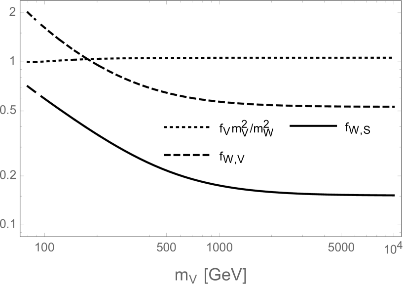
Figure 3: $f_{V}m_{V}^{2}/m_{W}^{2}$, $f_{W,S}$ and $f_{W,V}$ as functions of the $SU(2)_{R}$ scale $m_{V}$.

Hence, the large coupling product $g_{hWX}g_{ZWX}$ may give significant effects on the total amplitude of the decay $h\rightarrow Z\gamma$. But the contributions arising from this part were omitted in the literature, even with well known-models such as the left-right models and the Higgs Triplet Models (HTM).

In the original LR models reviewed in gaugExtent221 , $g_{ZWW^{\prime}}\sim(m_{W}/m_{W^{\prime}})^{2}$, lower bounds of few TeV for heavy gauge boson mass $m_{W^{\prime}}$ were concerned from recent experiments at LHC Aaboud:2018vgh . As a result, its contributions may be small. In contrast, recent versions introducing different assignments of fermions representations to explain latest experimental data of anomalies in $B$ meson decays allow lower values of $m_{W^{\prime}}$ near 1 TeV lowmwp ; Boucenna:2016qad .

Interesting studies on new charged gauge bosons $W^{\prime}$ in left-right models Dobrescu:2015qna ; Dobrescu:2015jvn ; Dobrescu:2015yba indicated that the couplings $W^{\prime}Wh,\,W^{\prime}WZ,W^{\prime}H^{\pm}Z$ result in important decays of $W^{\prime\pm}$, which are being hunted at LHC. These coupling also contribute to the decay $h\rightarrow Z\gamma$. The gauge bosons of the gauge groups $SU(2)_{L,R}$ and $U(1)_{B-L}$ are $W^{a}_{L,R\mu}$ ($a=1,2,3$) and $A_{B-L\mu}$ Dobrescu:2015jvn , respectively. The Higgs sector consists of one bidoublet $\Sigma$ whose breaks the electroweak scale, and a $SU(2)_{R}$ multiplet whose breaks the $SU(2)_{R}\times U(1)_{B-L}$ scale. Apart from the SM-like gauge bosons $Z_{\mu}$, $W^{\pm}_{\mu}$, and photon $A_{\mu}$, the left-right models predict new heavy gauge bosons including $W^{\prime\pm}$ and $Z^{\prime}$ with masses $m_{W^{\prime}}$ and $m_{Z^{\prime}}$, respectively. The bidoublet contributes mainly to the SM-like Higgs boson, Goldstone bosons of $Z$ and $W^{\pm}$, and a pair of singly charged Higgs $H^{\pm}$ that couple with the SM-like Higgs boson.

Relevant vertex factors are summarized in Table 2. The details of the models and calculations are given in Appendix C.

Vertex	SM	LR  Dobrescu:2015qna ; Dobrescu:2015yba
$g_{hWW}\,g_{ZWW}$	$g^{2}\,m_{W}\,c_{W},$	$g_{L}^{2}\,m_{W}c_{W}\sin(\beta-\alpha)$
$g_{hW^{\prime}W}g_{ZWW^{\prime}}$	$-$	$g_{L}g_{R}\,m_{W}\cos(\beta+\alpha)\frac{s_{\theta_{+}}}{c_{W}}$
$g_{hW^{\prime}W^{\prime}}g_{ZW^{\prime}W^{\prime}}$	$-$	$-g^{2}_{R}\,m_{W}\,\sin(\beta-\alpha)\frac{s^{2}_{W}}{c_{W}}$
$g_{hW^{+}H^{-}}g_{ZW^{-}H^{+}}$	$-$	$-\frac{g^{2}_{R}}{2}\,m_{W}\,c_{W}\sin(\beta+\alpha)\cos(2\beta)s^{2}_{\theta_{+}}$
$g_{hW^{\prime+}H^{-}}g_{ZW^{\prime-}H^{+}}$	$-$	$-\frac{g^{2}_{R}}{2}\,m_{W}\,c_{W}\sin(\beta+\alpha)\cos(2\beta)$

Table 2: Vertex factors involved charged gauge and Higgs bosons contributing to one loop amplitude of the SM-like Higgs decay $h\rightarrow Z\gamma$ in the LR model with $g\equiv g_{L}$ and $s_{\theta_{+}}\simeq\tan{\theta_{+}}=\frac{g_{R}}{g_{L}}\times\sin(2\beta)\epsilon^{2}$, and $\epsilon=m_{W}/m_{W^{\prime}}$.

We have used the condition $\alpha=\beta-\pi/2$ to guarantee that the coupling $hWW$ is the same as that in the SM. We ignore all suppressed terms having factors with orders larger than $\mathcal{O}(\epsilon^{2})$, where $\epsilon=m_{W}/m_{W^{\prime}}$ and $m_{W^{\prime}}$ is the new heavy gauge boson mass, which can be considered as the breaking scale of the $SU(2)_{R}$ group. The couplings of the SM-like Higgs boson we discuss here are consistent with those in Ref. Dev:2016dja ; Dobrescu:2015jvn ; Dobrescu:2015yba ; Jinaru:2013eya . The triple gauge couplings are also consistent with Refs. gaugExtent221 ; Vijcouple . Because they are not affected by the fermion assignments, they can be considered in the general case which does not depend on the recent experimental limit.

With the above assumptions, the couplings of the SM-like Higgs boson are nearly the same as those in the SM. The decay $h\rightarrow Z\gamma$ has contributions associated with charged gauge bosons estimated as follows,

$$\frac{F^{\mathrm{LR}}_{21,WWW}}{F^{\mathrm{SM}}_{21,W}} \simeq 1,\quad\frac{F^{\mathrm{LR}}_{21,W^{\prime}W^{\prime}W^{\prime}}}{F^{\mathrm{SM}}_{21,W}}\sim-\frac{g_{R}^{2}s^{2}_{W}}{g_{L}^{2}c^{2}_{W}}\epsilon^{2},$$

$$\frac{F^{\mathrm{LR}}_{21,WW^{\prime}W^{\prime}}+F^{\mathrm{LR}}_{21,W^{\prime}WW}}{F^{\mathrm{SM}}_{21,W}} \sim\frac{g_{R}^{2}\sin^{2}(2\beta)}{2g_{L}^{2}c^{2}_{W}}\epsilon^{2},\quad\frac{F^{\mathrm{LR}}_{21,HW^{\prime}W^{\prime}}+F^{\mathrm{LR}}_{21,W^{\prime}HH}}{F^{\mathrm{SM}}_{21,W}}\sim\frac{g_{R}^{2}\cos^{2}(2\beta)}{2g_{L}^{2}}\epsilon^{2},$$ (29)

where $\epsilon\equiv m_{W}/m_{W^{\prime}}$ and $\alpha\simeq\beta-\pi/2$. We can see that all quantities listed in (V) have the same order, although some of them are affected by the tiny mixing parameter $s_{\theta_{+}}=\mathcal{O}(\epsilon^{2})$ between two charged gauge bosons. Hence all of them must be taken into account. This argument is different from previous treatment where only $F^{\mathrm{LR}}_{21,W^{\prime}W^{\prime}W^{\prime}}$ was mentioned hzgalr1 ; hzgalr2 ; Maiezza:2016bzp . The recent lower bounds of the $SU(2)_{R}$ scale give $\epsilon^{2}\leq\mathcal{O}(10^{-3})$, implying that the heavy charged Higg and gauge contributions discussed here are suppressed. But the calculation is very useful for further investigation in many other gauge extensions allowing lower new breaking scales, for example, the models belonging to the class of breaking pattern I mentioned in Ref. Vijcouple , or recent models with breaking pattern II Boucenna:2016qad ; lowmwp .

The effects of heavy charged Higgs boson $m_{H}$ from $F_{21,WSS}$ and $F_{21,SWW}$ appear in simple models like the HTM, for a review see Accomando:2006ga . They even appear in the simple HTM models extended from the SM by adding only one Higgs triplet $\Delta$  Konetschny:1977bn ; Cheng:1980qt ; Schechter:1980gr . It contains one singly, another doubly charged scalar components, and a neutral one with non-zero expectation vacuum value (vev) denoted as $v_{\Delta}$. As a result, apart from the SM particles, the HTM predicts only new Higgs bosons. The factors $g_{hSW}$ and $g_{ZWS}$ arise from couplings of singly charged Higgs bosons $S^{\pm}$ with all gauge and neutral bosons. The correlation of the two decays $h\rightarrow\gamma\gamma$ and $h\rightarrow Z\gamma$ were investigated previously, but the contributions $F_{21,WSS}$ and $F_{21,SWW}$ mentioned here were ignored in Dev:2013ff because of the small product $g_{hSW}g_{ZWS}$. It is proportional to the small ratio $(v_{\Delta}/v)^{2}$ Arhrib:2011uy , where $v=246$ GeV. The requirement that the parameter $\rho=m_{W}^{2}/(m_{Z}^{2}c_{W}^{2})$ is close to 1 at the tree level forces $v_{\Delta}$ to be small with largest values of few GeV Dev:2013ff ; Aoki:2011pz ; Blunier:2016peh . But the tree-level deviation $\Delta\rho=\rho-1$ predicted by this model is negative, in contrast with the recent experimental results Patrignani:2016xqp . Hence, loop corrections should be included into this parameter, implying that small $v_{\Delta}$ is no longer necessary Gunion:1990dt ; Accomando:2006ga . Theoretical prediction for $v_{\Delta}\sim\mathcal{O}(10)$ GeV is still allowed Kanemura:2012rs . The recent experimental upper bound is $v_{\Delta}<25$ GeV Agrawal:2018pci . As a result, contributions from $F_{21,SWW}$ and $F_{21,WSS}$ to the SM-like Higgs boson decay $h\rightarrow Z\gamma$ can reach value of $F_{21,W}\times\mathcal{O}(10^{-2})$, which is still far from the sensitivity of the recent experiments. Hence, previous investigations  Dev:2013ff ; Arbabifar:2012bd ; Aoki:2011pz ignoring $F_{21,SWW}$ and $F_{21,WSS}$ in the one loop amplitude of the SM-like Higgs decay $h\rightarrow Z\gamma$ are still accepted.

On the other hand, heavy neutral bosons $H$ predicted by many BSM may have large $g_{HWS}\,g_{ZWS}$, for example the HTM Arhrib:2011uy . In this case, contributions of $F_{21,SWW}$, $F_{21,WSS}$ can reach the significant values of $F_{21,WWW}\times\mathcal{O}(v_{\Delta}/v)=F_{21,WWW}\times\mathcal{O}(10^{-1})$ in the decay Br$(H\rightarrow Z\gamma)$ but they were ignored in previous works Arbabifar:2012bd ; Chabab:2014ara ; Blunier:2016peh . The formulas we introduced in this work should be used for improved calculations of the mentioned decay rates.

VI Conclusions

The decay $h\rightarrow Z\gamma$ attracts now a great interest from both theoretical and experimental sides. It should be observed and studied soon by the LHC experiments. If a deviation from the SM prediction is found, it will be associated with new physics implying additional contributions from exotic particles in many BSM models. In this paper, we have introduced the general analytic formulas expressing one-loop contributions from scalars, fermions, and gauge bosons to the amplitude of the decay $h\rightarrow Z\gamma$. In addition, we proved that our results can be used to calculate the amplitude of the charged Higgs decays $H^{\pm}\rightarrow W^{\pm}\gamma$ which exist in many BSM models. Although some of these formulas were derived earlier by other groups, the general forms were not concerned, in particular, the contributions related to new gauge boson loops. Our formulas are applicable to many well-known gauge extended versions of the SM, as we discussed in detail. We stress that all one-loop contributions with gauge bosons involved are calculated explicitly using the unitary gauge, so that the readers can cross-check our results. Our final results are written in a convenient form. Namely, they are presented in terms of the standard Passarino-Veltman functions which can be evaluated numerically with the help of the LoopTools library. The analytic forms of these PV functions were also discussed, so that our results can be identified with well known formulas in several special cases as well as implemented into other numerical packages. Our results were checked to be mainly consistent with several recent calculations in some specific BSM models, except the contributions from diagrams containing two different virtual gauge bosons. We believe that our results will be useful for further studies of loop-induced decays of neutral and charged Higgs bosons $H\rightarrow Z\gamma,W\gamma$, which have not been yet treated in many well-known BSM models.

Appendix A PV functions in LoopTools

A.1 Definitions, notations and analytic formulas

We use the notations for the Passarino-Veltman functions from the LoopTools library LoopTools :

$$A^{(i)}_{0,\mu} =A_{0,\mu}(k_{i}^{2};m_{i+1}^{2})\equiv\frac{(2\pi\mu)^{4-d}}{i\pi^{2}}\int\frac{d^{d}q\,\left\{1,\,q_{\mu},\right\}}{D_{i}},\,i=0,1,2,$$

$$B^{(i)}_{0,\,\mu,\,\mu\nu} =B_{0,\mu}(k_{i}^{2};m_{1}^{2},m_{i+1}^{2})\equiv\frac{(2\pi\mu)^{4-d}}{i\pi^{2}}\int\frac{d^{d}q\,\left\{1,\,q_{\mu},\,q_{\mu}q_{\nu}\right\}}{D_{0}D_{i}},\,i=1,2,$$

$$C_{0,\mu,\mu\nu} =C_{0,\mu,\mu\nu}(p_{1}^{2},p_{2}^{2},(p_{1}+p_{2})^{2};m_{1}^{2},m_{2}^{2},m_{3}^{2})\equiv\frac{(2\pi\mu)^{4-d}}{i\pi^{2}}\int\frac{d^{d}q\,\left\{1,\,q_{\mu},\,q_{\mu}q_{\nu}\right\}}{D_{0}D_{1}D_{2}},$$ (30)

where $d=4-2\epsilon$ ($\epsilon\rightarrow 0$) is the integral dimension, $D_{i}=(q+k_{i})^{2}-m_{i+1}^{2}$,$k_{0}=0$, $k_{1}=-p_{1}$, $k_{2}=-(p_{1}+p_{2})$, $i=0,1,2$. In our case, we always have $m_{3}=m_{2}$.

Denoting $\Delta_{\epsilon}=\frac{1}{\epsilon}+\ln(4\pi\mu^{2})-\gamma_{E}$, it is well-known that peskin ; aBfunc

$$A_{0}^{(0)} =m_{1}^{2}(\Delta_{\epsilon}-\ln m_{1}^{2}+1),\quad A_{0}^{(1,2)}=m_{2}^{2}(\Delta_{\epsilon}-\ln m_{2}^{2}+1),\quad A^{(i)}_{\mu}=-A^{(i)}_{0}k_{i\mu},\quad$$ (31)

Based on the LoopTools notations LoopTools , functions $B^{(i)}_{0,\mu,\mu\nu}$ and $C_{0,\mu,\mu\nu}$ are written as

$$B^{(i)}_{\mu} =B^{(i)}_{1}k_{i\mu},$$

$$B^{(i)}_{\mu\nu} =B^{(i)}_{00}g_{\mu\nu}+B^{(i)}_{11}k_{i\mu}k_{i\nu},$$

$$C_{\mu} =C_{1}k_{1\mu}+C_{2}k_{2\mu},$$

$$C_{\mu\nu} =C_{00}g_{\mu\nu}+C_{11}k_{1\mu}k_{1\nu}+C_{12}(k_{1\mu}k_{2\nu}+k_{2\mu}k_{1\nu})+C_{22}k_{2\mu}k_{2\nu}.$$ (32)

There is another case where we have to change the integration variable $q\rightarrow q^{\prime}=q+k_{1}$ to get the standard form defined by (30):

$$B^{(12)}_{0,\mu,\mu\nu} \equiv B_{0,\mu,\mu\nu}(k_{1}^{2},k_{2}^{2};m_{2}^{2},m_{2}^{2})=\frac{(2\pi\mu)^{4-d}}{i\pi^{2}}\int\frac{d^{d}q\,\left\{1,\,q_{\mu},\,q_{\mu}q_{\nu}\right\}}{D_{1}D_{2}}$$

$$=\frac{(2\pi\mu)^{4-d}}{i\pi^{2}}\int\frac{d^{d}q\,\left\{1,\,q_{\mu}-k_{1\mu},\,(q_{\mu}-k_{1\mu})(q_{\nu}-k_{1\nu})\right\}}{(q^{2}-m_{2}^{2})\left[(q+k_{2}-k_{1})^{2}-m_{2}^{2}\right]}.$$ (33)

Then we can use the scalar coefficients $B^{(12)}_{0}$, $B^{(12)}_{1}$, and $B^{(12)}_{11}$ with the standard definitions, where $k_{2}-k_{1}=-p_{2}$,

$$B_{0,\mu,\mu\nu}((k_{2}-k_{1})^{2};m_{2}^{2},m_{2}^{2}) =\frac{(2\pi\mu)^{4-d}}{i\pi^{2}}\int\frac{d^{d}q\,\left\{1,\,q_{\mu},\,q_{\mu}q_{\nu}\right\}}{(q^{2}-m_{2}^{2})\left[(q+k_{2}-k_{1})^{2}-m_{2}^{2}\right]},$$

$$=B^{(12)}_{0},\,-B^{(12)}_{1}p_{2\mu},\,B^{(12)}_{00}g_{\mu\nu}+B^{(12)}_{11}p_{2\mu}p_{2\nu}.$$ (34)

Inserting these into (33) we get with $k_{1}=-p_{1}$ and $p_{2}^{2}=0$

$$3B^{(12)}_{11} =-2B^{(12)}_{1}=B^{(12)}_{0}=\Delta_{\epsilon}-\ln(m_{2}^{2}),\quad B^{(12)}_{00}=\frac{m_{2}^{2}}{2}\left(1+B^{(12)}_{0}\right),$$

$$B^{(12)}_{\mu} =\frac{B^{(12)}_{0}}{2}p_{2\mu}+B^{(12)}_{0}p_{1\mu},$$

$$B^{(12)}_{\mu\nu} =\frac{m_{2}^{2}}{2}\left(1+B^{(12)}_{0}\right)g_{\mu\nu}+\frac{B^{(12)}_{0}}{3}p_{2\mu}p_{2\nu}+\frac{B^{(12)}_{0}}{2}\left(p_{2\mu}p_{1\nu}+p_{1\mu}p_{2\nu}\right)+B^{(12)}_{0}p_{1\mu}p_{1\nu}.$$ (35)

For two other cases we get

$$B^{(i)}_{0} \equiv B^{(12)}_{0}+2-\sum_{\sigma=\pm}\left(1-\frac{1}{x_{i\sigma}}\right)\ln(1-x_{\sigma}),$$

$$B^{(i)}_{1} \equiv\frac{1}{2k_{i}^{2}}\left[A^{(0)}_{0}-A^{(i)}_{0}-(m_{1}^{2}-m_{2}^{2}+k^{2}_{i})B^{(i)}_{0}\right],$$ (36)

where $k_{1}^{2}=m_{Z}^{2}$, $k_{2}^{2}=m_{h}^{2}$, and $x_{i\sigma}$ are the roots of the equation $m_{2}^{2}x^{2}-(m_{2}^{2}-m_{1}^{2}+k_{i}^{2})x+k_{i}^{2}+i\epsilon=0$. The forms of $B^{(i)}_{0,1}$ used for numerical investigation are well-known, see e.g. aBfunc .

The $C_{0}$ function with $m_{3}=m_{2}$ has a simple form hzgamssm :

$$C_{0}=\frac{1}{k_{1}^{2}-k_{2}^{2}}\sum_{i=1}^{2}\sum_{\sigma=\pm}(-1)^{i}\mathrm{Li}_{2}\left[\frac{2k_{i}^{2}}{m_{2}^{2}-m_{1}^{2}+k_{i}^{2}+\sigma\lambda^{1/2}(k_{i}^{2},m_{1}^{2},m_{2}^{2})}\right],$$ (37)

where $\lambda(x,y,z)=x^{2}+y^{2}+z^{2}-2xy-2yz-2xz$. This formula is also consistent with LoopTools and C0f , where notations are changed as $(m_{1}^{2},m_{2}^{2},m_{F}^{2},m_{B}^{2})\rightarrow(k_{1}^{2},k_{2}^{2},m_{1}^{2},m_{2}^{2})$. The $C_{i,ij}$ functions are found based on the reduction technique aBfunc . Their explicit forms used in this work are C0f

$$C_{1} =\frac{(m_{h}^{2}+m_{Z}^{2})\left(B_{0}^{(1)}-B^{(12)}_{0}\right)-2m_{h}^{2}\left(B_{0}^{(2)}-B_{0}^{(12)}\right)}{(m_{h}^{2}-m_{Z}^{2})^{2}}+\frac{f_{2}C_{0}}{m_{Z}^{2}-m_{h}^{2}},$$

$$C_{2} =\frac{(m_{h}^{2}+m_{Z}^{2})\left(B_{0}^{(2)}-B^{(12)}_{0}\right)-2m_{Z}^{2}\left(B_{0}^{(1)}-B_{0}^{(12)}\right)}{(m_{h}^{2}-m_{Z}^{2})^{2}}-\frac{f_{1}C_{0}}{m_{Z}^{2}-m_{h}^{2}},$$

$$C_{22} =\frac{\left[f_{2}\left(-3m_{h}^{4}+m_{Z}^{4}-4m_{Z}^{2}m_{h}^{2}\right)+4m_{h}^{6}-4m_{Z}^{4}m_{h}^{2}\right]B^{(2)}_{0}}{2m_{h}^{2}\left(m_{Z}^{2}-m_{h}^{2}\right)^{3}}$$

$$+\frac{3f_{1}m_{Z}^{2}B^{(1)}_{0}}{(m_{Z}^{2}-m_{h}^{2})^{3}}-\frac{\left[f_{1}+f_{2}+2(m_{Z}^{2}-m_{h}^{2})\right]B^{(12)}_{0}}{2(m_{Z}^{2}-m_{h}^{2})^{2}}+\frac{(f_{1}^{2}+2m_{2}^{2}m_{Z}^{2})C_{0}}{(m_{Z}^{2}-m_{h}^{2})^{2}}$$

$$-\frac{(m_{Z}^{2}+m_{h}^{2})\left(A^{(1)}_{0}-A^{(0)}_{0}\right)}{2m_{h}^{2}(m_{Z}^{2}-m_{h}^{2})^{2}}+\frac{m_{Z}^{2}}{(m_{Z}^{2}-m_{h}^{2})^{2}},$$

$$C_{12} =-\frac{\left[f_{2}(5m_{Z}^{2}+m_{h}^{2})+m_{Z}^{4}-m_{h}^{4}\right]B^{(1)}_{0}}{2(m_{Z}^{2}-m_{h}^{2})^{3}}+\frac{\left[f_{1}(5m_{h}^{2}+m_{Z}^{2})+m_{h}^{4}-m_{Z}^{4}\right]B^{(2)}_{0}}{2(m_{Z}^{2}-m_{h}^{2})^{3}}$$

$$+\frac{(2m_{2}^{2}-2m_{1}^{2}+m_{Z}^{2}+m_{h}^{2})B^{(12)}_{0}}{2(m_{Z}^{2}-m_{h}^{2})^{2}}-\frac{\left[f_{1}f_{2}+m_{2}^{2}(m_{Z}^{2}+m_{h}^{2})\right]C_{0}}{(m_{Z}^{2}-m_{h}^{2})^{2}}$$

$$+\frac{A^{(1)}_{0}-A^{(0)}_{0}}{(m_{Z}^{2}-m_{h}^{2})^{2}}-\frac{m_{Z}^{2}+m_{h}^{2}}{2(m_{Z}^{2}-m_{h}^{2})^{2}},$$ (38)

where $f_{i}=m_{2}^{2}-m_{1}^{2}+k_{i}^{2}$. Some combinations which appear commonly in our calculations are

$$C_{1}+C_{2} =-\frac{B^{(1)}_{0}-B^{(2)}_{0}}{m_{Z}^{2}-m_{h}^{2}}-C_{0},$$

$$C_{12}+C_{22}+C_{2} =\frac{(-m_{1}^{2}+m_{2}^{2}+m_{Z}^{2})(B^{(1)}_{0}-B^{(12)}_{0})}{2(m_{Z}^{2}-m_{h}^{2})^{2}}$$

$$+\frac{\left[(m_{1}^{2}-m_{2}^{2})(2m_{h}^{2}-m_{Z}^{2})-m_{Z}^{2}m_{h}^{2}\right](B^{(2)}_{0}-B^{(12)}_{0})}{2m_{h}^{2}(m_{Z}^{2}-m_{h}^{2})^{2}}$$

$$+\frac{m_{2}^{2}C_{0}}{m_{Z}^{2}-m_{h}^{2}}+\frac{m_{1}^{2}-m_{2}^{2}+m_{h}^{2}-m_{1}^{2}\ln(m_{1}^{2}/m_{2}^{2})}{2m_{h}^{2}(m_{Z}^{2}-m_{h}^{2})}.$$ (39)

A.2 Analytic formulas in special case of $m_{1}=m_{2}=m$

In the case of equal masses, we can use the following well-known functions hzgamssm ; HzgaTHD ; GMmodel

$$g(x) =\left\{\begin{array}[]{cc}\sqrt{x-1}\arcsin\sqrt{\frac{1}{x}}&x\geq 1,\\ \frac{\sqrt{1-x}}{2}\left(-i\pi+\ln\frac{1+\sqrt{1-x}}{1-\sqrt{1-x}}\right)&x<1\\ \end{array}\right.,$$ (42)

$$f(x) =\left\{\begin{array}[]{cc}\arcsin^{2}\sqrt{\frac{1}{x}}&x\geq 1,\\ -\frac{1}{4}\left(-i\pi+\ln\frac{1+\sqrt{1-x}}{1-\sqrt{1-x}}\right)^{2}&x<1\\ \end{array}\right.,$$ (45)

$$I_{1}(x,y) =\frac{xy}{2(x-y)}+\frac{x^{2}y^{2}}{2(x-y)^{2}}\left[f(x)-f(y)\right]+\frac{x^{2}y}{(x-y)^{2}}\left[g(x)-g(y)\right],$$ (46)

$$I_{2}(x,y) =-\frac{xy}{2(x-y)}\left[f(x)-f(y)\right].$$ (47)

Defining $t_{1}=t_{z}=4m^{2}/m_{Z}^{2}$ and $t_{2}=t_{h}=4m^{2}/m_{h}^{2}$, the PV functions involved with this work can be written as

$$B^{(i)}_{0} =B^{(12)}_{0}+2-2g(t_{i}),$$ (48)

$$C_{0} =-\frac{I_{2}(t_{2},t_{1})}{m^{2}},$$ (49)

$$C_{1}+C_{2} =\frac{B^{(1)}_{0}-B^{(2)}_{0}}{m_{Z}^{2}-m_{h}^{2}}-C_{0},$$

$$C_{12}+C_{22}+C_{2} =\frac{m_{Z}^{2}(B^{(1)}_{0}-B^{(2)}_{0})}{2(m_{Z}^{2}-m_{h}^{2})^{2}}+\frac{m^{2}C_{0}}{m_{Z}^{2}-m_{h}^{2}}+\frac{1}{2(m_{Z}^{2}-m_{h}^{2})}=\frac{I_{1}(t_{2},t_{1})}{4m^{2}}.$$ (50)

The $B^{(i)}_{0}$ in eq. (48) is derived from the general well-know form, namely

$$B^{(i)}_{0} =B^{(12)}_{0}-\int_{0}^{1}dx\ln\left[1+4t_{i}^{-1}x(x-1)\right]=B^{(12)}_{0}-\int_{-\frac{1}{2}}^{\frac{1}{2}}dx\ln\left[4t_{i}^{-1}x^{2}+1-t_{i}^{-1}\right].$$

More intermediate steps, including integration by parts, are as follows

$$\int_{-\frac{1}{2}}^{\frac{1}{2}}dx\ln\left[4t_{i}^{-1}x^{2}+1-t_{i}^{-1}\right] =-\int_{-\frac{1}{2}}^{\frac{1}{2}}\frac{8t_{i}^{-1}x^{2}\,dx}{4t_{i}^{-1}x^{2}+1-t_{i}^{-1}}=-2+\int_{-\frac{1}{2}}^{\frac{1}{2}}\frac{2\,dx}{\frac{4x^{2}}{t_{i}-1}+1}=-2+2g(t_{i}).$$

Appendix B Details of amplitude calculation

For completeness, we present some more detailed steps to obtain the formulas of $M_{(5)\mu\nu}$ and $M_{(5+6)\mu\nu}$ in Eqs. (11) and (12). Also, the contribution from diagram 1 in figure 1 will be discussed.

Using the replacements in Eq. (10) to calculate the $F_{21}$ factor in $M_{(5)\mu\nu}$, we get

$$V_{1\mu\beta\lambda} =g_{\alpha\beta}\left(g^{\alpha^{\prime}}_{\beta}-\frac{q_{\beta}q^{\alpha^{\prime}}}{m_{1}^{2}}\right)\left[(q+q_{1})_{\mu}g_{\alpha^{\prime}\lambda}-(q+p_{1})_{\lambda}g_{\alpha^{\prime}\mu}-(q_{1}-p_{1})_{\alpha^{\prime}}g_{\mu\lambda}\right]$$

$$=(q+q_{1})_{\mu}g_{\beta\lambda}-(q+p_{1})_{\lambda}g_{\mu\beta}-(q_{1}-p_{1})_{\beta}g_{\mu\lambda}-\frac{(q+q_{1})_{\mu}q_{\beta}q_{\lambda}}{m_{1}^{2}}$$

$$+\frac{(q+p_{1})_{\lambda}q_{\beta}q_{\mu}}{m_{1}^{2}}+\frac{(q_{1}-p_{1})qq_{\beta}g_{\lambda\mu}}{m_{1}^{2}}$$

$$\rightarrow 2q_{\mu}g_{\beta\lambda}-(q+p_{1})_{\lambda}g_{\mu\beta}-(q_{1}-p_{1})_{\beta}g_{\mu\lambda}+\frac{q_{\beta}}{m_{1}^{2}}\left[-q_{\mu}q_{1\lambda}+(q_{1}^{2}-m_{Z}^{2})g_{\mu\lambda}\right]$$

$$\equiv V_{1,1\mu\beta\lambda}+\frac{1}{m^{2}_{1}}\times V_{1,2\mu\beta\lambda},$$ (51)

where we have used $p_{1}^{2}=m_{Z}^{2}$, $p_{2}^{2}=0$, $q.(q_{1}-p_{1})=(q_{1}+p_{1}).(q_{1}-p_{1})=q_{1}^{2}-p_{1}^{2}$, $q_{1}.(q_{2}-p_{2})=q_{2}^{2}$ etc. The arrow means that replacements (10) have been applied. And we will apply them automatically from now on. Similarly, we can prove that

$$V_{2\nu}^{\beta\lambda}\rightarrow V_{2,1\nu}^{\beta\lambda}+\frac{1}{m^{2}_{2}}\times V_{2,2\nu}^{\beta\lambda}+\frac{1}{m^{4}_{2}}\times V_{2,3\nu}^{\beta\lambda},$$ (52)

where

$$V_{2,1\nu}^{\beta\lambda} =-(q_{1}+p_{2})^{\beta}\delta_{\nu}^{\lambda}-(q_{2}-p_{2})^{\lambda}\delta_{\nu}^{\beta}+2q_{1\nu}g^{\beta\lambda},$$

$$V_{2,2\nu}^{\beta\lambda} =q_{1}^{\lambda}\left(\delta^{\beta}_{\nu}q_{2}^{2}+q_{1\nu}(q_{1}+p_{2})^{\beta}-2q_{1\nu}q_{1}^{\beta}\right)+q_{2}^{\beta}\left(\delta^{\lambda}_{\nu}q_{1}^{2}-q_{2\nu}p_{2}^{\lambda}-q_{1\nu}q_{2}^{\lambda}\right),$$

$$\rightarrow q_{1}^{\lambda}\delta^{\beta}_{\nu}q_{2}^{2}+q_{2}^{\beta}\delta^{\lambda}_{\nu}q_{1}^{2}-2q_{1\nu}q_{1}^{\lambda}q_{2}^{\beta},$$

$$V_{2,3\nu}^{\beta\lambda} =-(q_{1}.p_{2})q_{1}^{\lambda}q_{2}^{\beta}p_{2\nu}\rightarrow 0.$$ (53)

Now the part we need is written as follows

$$V_{1\mu\beta\lambda}V_{2\nu}^{\beta\lambda}\rightarrow(V_{1,1}V_{2,1})_{\mu\nu}+\frac{(V_{1,1}V_{2,2})_{\mu\nu}}{m_{2}^{2}}+\frac{(V_{1,2}V_{2,1})_{\mu\nu}}{m_{1}^{2}}+\frac{(V_{1,2}V_{2,2})_{\mu\nu}}{m_{1}^{2}m_{2}^{2}},$$ (54)

where

$$(V_{1,1}V_{2,1})_{\mu\nu} =2(2d-3)q_{\mu}q_{\nu}+(-4d+7)q_{\mu}p_{1\nu}-p_{2\mu}q_{\nu}+5p_{2\mu}p_{1\nu},$$

$$(V_{1,1}V_{2,2})_{\mu\nu} =q_{\mu}q_{\nu}\left[q^{2}+q_{1}^{2}+m_{h}^{2}-2m_{Z}^{2}\right]+q_{\mu}p_{1\nu}\left[-q^{2}-3q_{1}^{2}+q_{2}^{2}-m_{h}^{2}+2m_{Z}^{2}\right]$$

$$+p_{2\mu}q_{\nu}\left[-2q^{2}+q_{1}^{2}+2m_{Z}^{2}\right]+p_{2\mu}p_{1\nu}\left[2q^{2}+q_{1}^{2}-2m_{Z}^{2}\right],$$

$$(V_{1,2}V_{2,1})_{\mu\nu} =q_{\mu}\left[-q_{1\nu}(q.q_{2})+q_{\nu}q_{2}^{2}\right]+(q_{1}^{2}-m_{Z}^{2})\left(q_{\mu}q_{\nu}-2q_{\mu}p_{1\nu}+2p_{2\mu}q_{\nu}\right)$$

$$=q_{\mu}q_{\nu}\left[-\frac{q^{2}}{2}+q_{1}^{2}+\frac{q_{2}^{2}}{2}+\frac{m_{h}^{2}-2m_{Z}^{2}}{2}\right]$$

$$+q_{\mu}p_{1\nu}\left[\frac{q^{2}}{2}-2q_{1}^{2}+\frac{q^{2}_{2}}{2}+\frac{-m_{h}^{2}+4m_{Z}^{2}}{2}\right]+p_{2\mu}q_{\nu}\left[2q_{1}^{2}-2m_{Z}^{2}\right],$$

$$(V_{1,2}V_{2,2})_{\mu\nu} =-q_{\mu}q_{\nu}p_{1}^{2}q_{2}^{2}+q_{\mu}q_{1\nu}(q.q_{2})\left[2p_{1}^{2}-q_{1}^{2}\right]$$

$$=q_{\mu}q_{\nu}\left[-m_{Z}^{2}q_{2}^{2}+\frac{1}{2}(q^{2}+q_{2}^{2}-m_{h}^{2})\left(-q_{1}^{2}+2m_{Z}^{2}\right)\right]$$

$$-q_{\mu}p_{1\nu}\frac{1}{2}(q^{2}+q_{2}^{2}-m_{h}^{2})\left(-q_{1}^{2}+2m_{Z}^{2}\right).$$ (55)

From this, it is easy to derive the Eq. (11).

The amplitude corresponding to diagram 6 from figure 1 is

$$i\mathcal{M}_{(6)\mu\nu} =\int\frac{d^{d}q}{(2\pi)^{d}}(ig_{hV_{ij}}\,g_{\alpha\beta})\frac{-i}{D_{0}}\left(g^{\alpha\alpha^{\prime}}-\frac{q^{\alpha}q^{\alpha^{\prime}}}{m_{1}^{2}}\right)$$

$$\times(-ie\,Q~{}g_{ZV_{ij}})\left[2g_{\mu\nu}g_{\alpha^{\prime}\beta^{\prime}}-g_{\mu\nu}g_{\alpha^{\prime}\beta^{\prime}}-g_{\mu\nu}g_{\alpha^{\prime}\beta^{\prime}}\right]\frac{-i}{D_{2}}\left(g^{\beta\beta^{\prime}}-\frac{q_{2}^{\beta}q_{2}^{\beta^{\prime}}}{m_{2}^{2}}\right)$$

$$\rightarrow\left[e\,Q\,g_{hV_{ij}}~{}g_{ZV_{ij}}\right]\times\int\frac{d^{d}q}{(2\pi)^{d}}\frac{1}{D_{0}D_{2}}\times\frac{1}{m_{1}^{2}m_{2}^{2}}$$

$$\times\left[-2m_{1}^{2}q_{2\mu}q_{2\nu}-2m_{2}^{2}q_{\mu}q_{\nu}+(q.q_{2})(q_{2\mu}q_{\nu}+q_{\mu}q_{2\nu})\right].$$ (56)

Then it is easy to derive that

$$i\mathcal{M}_{(6)\mu\nu} \rightarrow\left[e\,Q\,g_{hV_{ij}}~{}g_{ZV_{ij}}\right]\int\frac{d^{d}q}{(2\pi)^{d}}\times\frac{1}{m_{1}^{2}m_{2}^{2}}$$

$$\times\left\{q_{\mu}q_{\nu}\left[\frac{1}{D_{2}}+\frac{1}{D_{0}}-\frac{m_{1}^{2}+m_{2}^{2}+m_{h}^{2}}{D_{0}D_{2}}\right]+q_{\mu}p_{1\nu}\left[-\frac{1}{2D_{2}}-\frac{1}{2D_{0}}+\frac{3m_{1}^{2}-m_{2}^{2}+m_{h}^{2}}{2D_{0}D_{2}}\right]\right.$$

$$\left.+p_{2\mu}q_{\nu}\left[-\frac{1}{2D_{2}}-\frac{1}{2D_{0}}+\frac{3m_{1}^{2}-m_{2}^{2}+m_{h}^{2}}{2D_{0}D_{2}}\right]+p_{2\mu}p_{1\nu}\left[\frac{-2m_{1}^{2}}{D_{0}D_{2}}\right]\right\}.$$ (57)

Contribution from the diagram 1 of figure 1 is

$$i\mathcal{M}_{(1)\mu\nu} =(-1)\times\int\frac{d^{d}q}{(2\pi)^{d}}\times\mathrm{Tr}\left[-i\left(Y_{hf_{ij}L}\,P_{L}+Y_{hf_{ij}R}\,P_{R}\right)\frac{i(q\!\!\!/_{2}+m_{2})}{D_{2}}\right.$$

$$\left.\times(ie\,Q\,\gamma_{\nu})\frac{i(q\!\!\!/_{1}+m_{2})}{D_{1}}\left[i\left(g^{*}_{Zf_{ij}L}\gamma_{\mu}\,P_{L}+g^{*}_{Zf_{ij}R}\gamma_{\mu}\,P_{R}\right)\right]\frac{i(q\!\!\!/+m_{1})}{D_{0}}\right]$$

$$=-e\,Q\int\frac{d^{d}q}{(2\pi)^{d}}\times\frac{1}{D_{0}D_{1}D_{2}}$$

$$\times\frac{1}{2}\mathrm{Tr}\left[\left(q\!\!\!/_{2}\gamma_{\nu}q\!\!\!/_{1}\gamma_{\mu}+m^{2}_{2}\gamma_{\mu}\gamma_{\nu}\right)\left(K^{+}_{LL,RR}-K^{-}_{LL,RR}\gamma_{5}\right)\right.$$

$$\left.+\left(q\!\!\!/_{2}\gamma_{\nu}\gamma_{\mu}q\!\!\!/+\gamma_{\nu}q\!\!\!/_{1}\gamma_{\mu}q\!\!\!/\right)\left(K^{+}_{LR,RL}+K^{-}_{LR,RL}\gamma_{5}\right)\right].$$

While the contribution of the corresponding diagram with opposite internal directions is

$$i\mathcal{M}^{\prime}_{(1)\mu\nu} =-e\,Q\int\frac{d^{d}q}{(2\pi)^{d}}\times\frac{1}{D_{0}D_{1}D_{2}}$$

$$\times\frac{1}{2}\mathrm{Tr}\left[\left(q\!\!\!/_{2}\gamma_{\nu}q\!\!\!/_{1}\gamma_{\mu}+m^{2}_{2}\gamma_{\mu}\gamma_{\nu}\right)\left(K^{+*}_{LL,RR}+K^{-*}_{LL,RR}\gamma_{5}\right)\right.$$

$$\left.+\left(q\!\!\!/_{2}\gamma_{\nu}\gamma_{\mu}q\!\!\!/+\gamma_{\nu}q\!\!\!/_{1}\gamma_{\mu}q\!\!\!/\right)\left(K^{+*}_{LR,RL}-K^{-*}_{LR,RL}\gamma_{5}\right)\right].$$

The sum of the two above diagrams gives the final result of $F_{21,f_{ijj}}$ and $f_{5,f_{ijj}}$ where the complex conjugation corresponds to the contribution from $\mathcal{M}^{\prime}_{(1)\mu\nu}$. Using the properties of the Dirac matrices, it is easy to find out the two expresions given in eq. (15).

Appendix C Gauge bosons and couplings in the left-right model $SU(2)_{L}\times SU(2)_{R}\times U(1)_{B-L}$

The model used here was introduced in Ref.  Dobrescu:2015jvn ; Dobrescu:2015yba , where many results we show here were introduced. The relations between the original gauge boson states and the physical ones $\{W^{\prime\pm}_{\mu},\,W^{\pm}_{\mu},A_{\mu},\,Z_{\mu},\,Z^{\prime}_{\mu}\}$ are

$$\begin{pmatrix}W^{\pm}_{R\mu}\\ W^{\pm}_{L\mu}\end{pmatrix} =\begin{pmatrix}c_{\theta_{+}}&s_{\theta_{+}}\\ -s_{\theta_{+}}&c_{\theta_{+}}\end{pmatrix}\begin{pmatrix}W^{\prime\pm}_{\mu}\\ W^{\pm}_{\mu}\end{pmatrix},$$

$$\begin{pmatrix}W^{3}_{L\mu}\\ W^{3}_{R\mu}\\ A_{B-L\mu}\\ \end{pmatrix} \simeq\begin{pmatrix}s_{W},&c_{W},&-c^{3}_{R}\frac{g_{R}}{g_{L}}\epsilon^{2}\\ s_{R}c_{W},&-s_{R}s_{W},&c_{R}\\ c_{R}c_{W},&-c_{R}s_{W},&-s_{R}\end{pmatrix}\begin{pmatrix}A_{\mu}\\ Z_{\mu}\\ Z^{\prime}_{\mu}\\ \end{pmatrix},$$ (58)

where $W^{\pm}_{L,R\mu}\equiv\frac{W^{1}_{L,R\mu}\mp iW^{2}_{L,R\mu}}{\sqrt{2}}$,

$$s_{\theta_{+}}=\frac{g_{R}}{g}\epsilon^{2}\sin 2\beta,\quad s_{R} \equiv\frac{g_{Y}}{g_{R}}=\frac{g_{L}t_{W}}{g_{R}},\quad\epsilon\equiv\frac{m_{W}}{m_{W^{\prime}}},\quad\quad m_{Z^{\prime}}=\frac{m_{W^{\prime}}}{c_{R}}.$$

We will keep the approximation up to the order $\mathcal{O}(\epsilon^{2})$, which gives $s^{2}_{\theta_{+}}=0$ and $c_{\theta_{+}}=1$.

Only the bidoublet Higgs $\Sigma\sim(2,2,0)$ contributes to the SM-like Higgs boson, namely

$$\Sigma=\begin{pmatrix}\Sigma^{0}_{1}&\Sigma^{+}_{2}\\ \Sigma^{-}_{1}&\Sigma^{0}_{2}\end{pmatrix}=\begin{pmatrix}v_{H}c_{\beta}-\frac{s_{\alpha}}{\sqrt{2}}h,&H^{+}c_{\beta}\\ H^{-}s_{\beta},&v_{H}s_{\beta}+\frac{c_{\alpha}}{\sqrt{2}}h\end{pmatrix},$$ (59)

where only the SM-like Higgs $h$ and charged Higgs bosons are kept. The SM-like gauge boson $W^{\pm}$ has mass $m_{W}\simeq g_{L}v_{H}/\sqrt{2}$.

The respective covariant derivative is gaugExtent221 ,

$$D_{\mu}\Sigma =\partial_{\mu}\Sigma-ig_{L}\frac{\sigma_{a}}{2}W^{a}_{L\mu}\Sigma+ig_{R}\Sigma\frac{\sigma_{a}}{2}W^{a}_{R\mu},$$

$$\equiv\partial_{\mu}\Sigma-\frac{ig_{L}}{2}P_{\Sigma\mu},$$ (60)

where $g_{L,R}$ and $W^{a}_{L,R\mu}$ $(a=1,2,3)$ are the gauge couplings and bosons of the groups $SU(2)_{L,R}$, $\sigma_{a}$ are Pauli matrices.

The kinetic term of the $\Sigma$ is

$$\mathcal{L}_{\Sigma}^{k} =\mathrm{Tr}\left[\left(D_{\mu}\Sigma\right)^{\dagger}\left(D^{\mu}\Sigma\right)\right]$$

$$=\mathrm{Tr}\left[\partial_{\mu}\Sigma^{\dagger}\left(\partial^{\mu}\Sigma\right)-\frac{ig_{L}}{2}\left[\partial_{\mu}\Sigma^{\dagger}\left(P^{\mu}\Sigma\right)-\left(P_{\mu}\Sigma\right)^{\dagger}(\partial^{\mu}\Sigma)\right]+\frac{g^{2}_{L}}{4}\left(P_{\mu}\Sigma\right)^{\dagger}\left(P^{\mu}\Sigma\right)\right],$$ (61)

which contains couplings of Higgs and gauge bosons. The part of the Lagrangian (C) giving couplings $hV^{+}V^{\prime-}$ is

$$\mathcal{L}(hV^{\pm}V^{\prime\mp}) =\frac{g^{2}_{L}}{2}\left[\left(\Sigma^{0*}_{1}\Sigma^{0}_{1}+\Sigma^{0*}_{2}\Sigma^{0}_{2}\right)\left(W^{+\mu}_{L}W^{-}_{L\mu}+\frac{g_{R}^{2}}{g_{L}^{2}}W^{+\mu}_{R}W^{-}_{R\mu}\right)\right.$$

$$\left.-2\frac{g_{R}}{g_{L}}\left(\Sigma^{0*}_{1}\Sigma^{0}_{2}W^{+\mu}_{L}W^{-}_{R\mu}+\Sigma^{0*}_{2}\Sigma^{0}_{1}W^{+\mu}_{R}W^{-}_{L\mu}\right)\right]$$

$$\rightarrow g_{L}m_{W}\sin(\beta-\alpha)h\left(W^{\mu}W^{-}_{\mu}+\frac{g_{R}^{2}}{g_{L}^{2}}W^{\prime+\mu}W^{\prime-}_{\mu}\right)$$

$$-g_{R}m_{W}\cos(\beta+\alpha)h\left(W^{+\mu}W^{\prime-}_{\mu}+W^{-\mu}W^{\prime+}_{\mu}\right),$$ (62)

where we keep only dominant contributions to the coefficients of the $hV^{+}V^{\prime-}$, i.e. we use the approximation $W\simeq W_{L}$ and $W^{\prime}\simeq W_{R}$.

The couplings $ZH^{\pm}V^{\mp}$ are

$$\mathcal{L}(ZH^{\pm}V^{\mp}) =-g_{R}m_{W}\cos(2\beta)\times W^{3}_{L\mu}(W^{+\mu}_{R}H^{-}+W^{-\mu}_{R}H^{+})$$

$$\simeq-g_{R}c_{W}m_{W}\cos(2\beta)\times Z_{\mu}\left(s_{\theta_{+}}W^{+\mu}H^{-}+W^{\prime+\mu}H^{-}+\mathrm{H.c.}\right),$$ (63)

where we used $c_{\theta_{+}}=1$ and $W^{3\mu}_{L}\rightarrow c_{W}Z^{\mu}$. This result is consistent with Dobrescu:2015jvn

The couplings $hH^{\pm}V^{\mp}$ are

$$\mathcal{L}(hH^{\pm}V^{\mp}) =-\frac{ig_{L}}{2}\mathrm{Tr}\left[\partial_{\mu}\Sigma^{\dagger}\left(P^{\mu}\Sigma\right)-\left(P_{\mu}\Sigma\right)^{\dagger}(\partial^{\mu}\Sigma)\right]$$

$$\rightarrow\frac{g_{L}}{2}\cos(\beta-\alpha)\left[(p_{0}-p_{-})_{\mu}W^{+\mu}_{L}H^{-}h-(p_{0}-p_{+})_{\mu}W^{-\mu}_{L}H^{+}h\right]$$

$$+\frac{g_{R}}{2}\sin(\beta+\alpha)\left[(p_{0}-p_{-})_{\mu}W^{+\mu}_{R}H^{-}h-(p_{0}-p_{+})_{\mu}W^{-\mu}_{R}H^{+}h\right],$$ (64)

where we have used $\partial_{\mu}\rightarrow-ip_{\mu}$; $p_{0,\pm}$ are momenta of the Higgs boson $h$ and $H^{\pm}$. The first line of the final result in (C) contains the factor $\cos(\beta-\alpha)\simeq\cos(\pi/2)=0$, because the matching condition with the SM coupling $hW^{+}W^{-}$ lead to $\beta=\alpha+\pi/2$. Using $W^{\pm}_{R\mu}\simeq W^{\prime\pm}_{\mu}+s_{\theta}W^{\pm}_{\mu}$, the second line is written in the physical gauge boson states as follows,

$$\mathcal{L}(hH^{\pm}V^{\mp}) =\frac{g_{R}}{2}\sin(\beta+\alpha)\left[(p_{0}-p_{-})_{\mu}\left(W^{\prime+\mu}+s_{\theta}W^{+\mu}\right)H^{-}h\right.$$

$$\left.-(p_{0}-p_{+})_{\mu}\left(W^{\prime-\mu}+s_{\theta}W^{-\mu}\right)H^{+}h\right].$$ (65)

The triplet couplings of three gauge bosons $ZVV^{\prime}$ are contained in the kinetic term of the non-abelian gauge bosons, namely gaugExtent221

$$\mathcal{L}^{k}_{g} =-\frac{1}{4}F^{a}_{L\mu\nu}F^{a\mu\nu}_{L}-\frac{1}{4}F^{a}_{R\mu\nu}F^{a\mu\nu}_{R},$$

$$F^{a}_{L,R\mu\nu} =\partial_{\mu}W^{a}_{L,R\nu}-\partial_{\nu}W^{a}_{L,R\mu}+g_{L,R}\epsilon^{abc}W^{b}_{L,R\mu}W^{c}_{L,R\nu}.$$ (66)

The triplet gauge couplings are derived as follows,

$$\mathcal{L}_{3g} =-g_{L}\epsilon^{abc}(\partial_{\mu}W^{a}_{L\nu})W^{b\mu}_{L}W^{c\nu}_{L}-g_{R}\epsilon^{abc}(\partial_{\mu}W^{a}_{R\nu})W^{b\mu}_{R}W^{c\nu}_{R}$$

$$=-ig_{L}c_{W}\left[Z^{\nu}\left(-\partial_{\mu}W^{+}_{L\nu}W^{-\mu}_{L}+\partial_{\mu}W^{-}_{L\nu}W^{+\mu}_{L}\right)+Z^{\mu}\left(\partial_{\mu}W^{+}_{L\nu}W^{-\nu}_{L}-\partial_{\mu}W^{-}_{L\nu}W^{+\nu}_{L}\right)\right.$$

$$\left.+\partial_{\mu}Z_{\nu}\left(-W^{+\mu}_{L}W^{-\nu}_{L}+W^{-\mu}_{L}W^{+\nu}_{L}\right)\right]-ig_{R}(-s_{R}s_{W})\times(L\rightarrow~{}R),$$ (67)

where we pay attention to only $Z$ couplings by replaced $W^{3}_{L}\rightarrow c_{W}Z$ and $W^{3}_{R}\rightarrow-s_{R}s_{W}Z$ in the last row of (C).

Now based on the Feynman rules, the vertex factor of the coupling $Z^{\alpha}W^{+\mu}W^{-\nu}$ defined as $-ig_{ZW^{+}W^{-}}\Gamma_{\alpha\mu\nu}(p_{0},p_{+},p_{-})$ can be derived by taking the limit $W^{\pm}_{L}\rightarrow W^{\pm}$. As a result, we obtain $g_{ZW^{+}W^{-}}\simeq g_{L}c_{W}$. Similarly, the coupling $Z^{\alpha}W^{\prime+\mu}W^{\prime-\nu}$ with the vertex factor $-ig_{ZW^{\prime+}W^{\prime-}}\Gamma_{\alpha\mu\nu}(p_{0},p_{+},p_{-})$ gives $g_{ZW^{\prime+}W^{\prime-}}\simeq-g_{R}s_{R}s_{W}=-g_{Y}s_{W}=-g_{L}s^{2}_{W}/c_{W}$.

Using $W^{+}_{L\mu}W^{-}_{L\nu}\rightarrow-s_{\theta_{+}}c_{\theta_{+}}W^{\prime+}_{\mu}W^{-}_{\nu}+\mathrm{H.c.}$ and $W^{+}_{R\mu}W^{-}_{R\nu}\rightarrow s_{\theta_{+}}c_{\theta_{+}}W^{\prime+}_{\mu}W^{-}_{\nu}+\mathrm{H.c.}$, the couplings $Z^{\alpha}W^{\prime+\mu}W^{-\nu}$ and $Z^{\alpha}W^{+\mu}W^{\prime-\nu}$ give $g_{ZW^{+}W^{\prime-}}=g_{ZW^{\prime+}W^{-}}=-s_{\theta_{+}}c_{\theta_{+}}\left(g_{L}c_{W}+g_{R}s_{R}s_{W}\right)\simeq-g_{L}s_{\theta_{+}}/c_{W}$, respectively.

References

- (1) ATLAS collaboration, G. Aad et al., Phys. Lett. B 716 (2012) 1 [arXiv:1207.7214].
- (2) CMS collaboration, S. Chatrchyan et al., Phys. Lett. B 716 (2012) 30 [arXiv:1207.7235].
- (3) G. Aad et al. [ATLAS and CMS Collaborations], JHEP 1608 (2016) 045, [arXiv:1606.02266 [hep-ex]].
- (4) CMS Collaboration, V. Khachatryan et al., Eur. Phys.J. C 75 (2015) 212 [arXiv:1412.8662].
- (5) R. Bonciani, V. D. Duca, H. Frellesvig, J.M. Henn, F. Moriello, V. A. Smirnov, JHEP 08 (2015) 108 [arXiv:1505.00567].
- (6) L. Bergstrom and G. Hulth, Nucl. Phys. B 259 (1985) 137 [err. B276 (1986) 744].
- (7) J. F. Gunion, G. L. Kane, J. Wudka, Nucl. Phys. B 299 (1988) 231.
- (8) D. Y. Bardin, P. K. Khristova and B. M. Vilensky, Sov. J. Nucl. Phys. 54 (1991) 833 [Yad. Fiz. 54 (1991) 1366].
- (9) A. Djouadi, V. Driesen, W. Hollik, A. Kraft, Eur. Phys.J. C 1 (1998) 163 [hep-ph/9701342 ].
- (10) J. F. Gunion, H. E. Haber, G. L. Kane, and S. Dawson, The Higgs Hunter’s Guide, Westview Press (2000).
- (11) J. Cao, L. Wu, P. Wu and J. M. Yang, JHEP 1309 (2013) 043 [arXiv:1301.4641 [hep-ph]].
- (12) G. Belanger, V. Bizouard and G. Chalons, Phys. Rev. D 89 (2014) no.9, 095023 [arXiv:1402.3522 [hep-ph]].
- (13) A. Hammad, S. Khalil and S. Moretti, Phys. Rev. D 92 (2015) no.9, 095008 [arXiv:1503.05408 [hep-ph]].
- (14) ATLAS Collaboration, M. Aaboud et al., JHEP 10 (2017) 112 [arXiv:1708.00212].
- (15) CMS Collaboration, A. M Sirunyan et al., Phys. Lett. B 772 (2017) 363 [arXiv:1612.09516].
- (16) CMS Collaboration V. Khachatryan et al., JHEP 01 (2017) 076 [arXiv:1610.02960].
- (17) J. M. No, M. Spannowsky, Phys. Rev. D 95 (2017) 075027 [arXiv:1612.06626].
- (18) S. T. Monfared, Sh. Fayazbakhsh , M. M. Najafabadi, Phys. Lett. B 762 (2016) 301.
- (19) D. Fontes, J.C. Romao, J. P. Silva, JHEP 12 (2014) 043, [arXiv:1408.2534].
- (20) C. Degrande, K. Hartling, H. E. Logan, Phys. Rev. D 96 (2017) 075013 [arXiv:1708.08753].
- (21) N. Bizot and M. Frigerio, JHEP 01 (2016) 036 [arXiv:1508.01645].
- (22) P. S. Bhupal Dev, D. K. Ghosh, N. Okada and I. Saha, JHEP 1303 (2013) 150, Erratum: [JHEP 1305 (2013) 049], [arXiv:1301.3453 [hep-ph]].
- (23) J. C. Pati and A. Salam, Phys. Rev. D 10 (1974) 275 [Erratum: Phys. Rev. D 11 (1975) 703].
- (24) R. N. Mohapatra, J. C. Pati, Phys. Rev. D 11 (1975) 2558.
- (25) R. N. Mohapatra, J. C. Pati, Phys. Rev. D 11 (1975) 566.
- (26) G. Senjanovic, R. N. Mohapatra, Phys. Rev. D 12 (1975) 1502.
- (27) R. N. Mohapatra, P. B. Pal, Phys. Rev. D 38 (1988) 2226.
- (28) G. Senjanovic, Nucl. Phys. B 153 (1979) 334.
- (29) M. Singer, J. W. F. Valle, and J. Schechter, Phys. Rev. D 22 (1980) 738.
- (30) J. W. F. Valle and M. Singer, Phys. Rev. D 28 (1983) 540.
- (31) F. Pisano and V. Pleitez, Phys. Rev. D 46 (1992) 410.
- (32) P. H. Frampton, Phys. Rev. Lett. 69 (1992) 2889.
- (33) R. Foot, H. N. Long, and T. A. Tran, Phys. Rev. D 50 (1994) 34 [hep-ph/9402243].
- (34) R. A. Diaz, R. Martinez, and F. Ochoa, Phys. Rev. D 72 (2005) 035018 [hep-ph/0411263].
- (35) A. J. Buras, F. De Fazio, J. Girrbach, and M. V. Carlucci, JHEP 02 (2013) 023.
- (36) L. T. Hue, L. D. Ninh, Mod. Phys. Lett. A 31 (2016) 1650062 [arXiv:1510.00302].
- (37) F. Pisano, V. Pleitez, Phys. Rev. D 51 (1995) 3865 [hep-ph/9401272].
- (38) H. N. Long, L. T. Hue, D. V. Loi, Phys. Rev. D 94 (2016) 015007 [arXiv:1605.07835].
- (39) R. Martinez, M. A. Perez, Nucl. Phys. B 347 (1990) 105.
- (40) R. Martinez, M. A. Perez, J. J. Toscano, Phys. Lett. B 234 (1990) 503.
- (41) G. Passarino and M. J. G. Veltman, Nucl. Phys. B 160 (1979) 151.
- (42) A. Denner, Fortsch. Phys. 41 (1993) 307 [arXiv:0709.1075].
- (43) T. Hahn, M. Perez-Victoria, Comput. Phys. Commun. 118 (1999) 153 [hep-ph/9807565].
- (44) S. Funatsu, H. Hatanaka, Y. Hosotani, Phys. Rev. D 92 (2015) 115003, Erratum: Phys. Rev. D 94 (2016) 019902.
- (45) M. E. Peskin and D. V. Schroeder, An in troduction to Quantum Field Theory, Westview Press, Perseus Books Group (1995).
- (46) G. Belanger, F. Boudjema, J. Fujimoto, T. Ishikawa, T. Kaneko, K. Kato, Y. Shimizu, Phys. Rept. 430 (2006) 117.
- (47) L. T. Hue, L. D. Ninh, T. T. Thuc, N. T. T. Dat, Eur. Phys. J. C 78 (2018) 128.
- (48) P. Duka, J. Gluza, M. Zralek, Annals Phys. 280 (2000) 336 [hep-ph/9910279].
- (49) A. Roitgrund, G. Eilam and S. Bar-Shalom, Comput. Phys. Commun. 203 (2016) 18 [arXiv:1401.3345 [hep-ph]].
- (50) L. T. Hue, A. B. Arbuzov, N. T. K. Ngan, H. N. Long, Eur. Phys. J. C 77 (2017) 346.
- (51) D.T. Binh, D. T. Huong, T. T. Huong, H. N. Long, D. V. Soa, J. Phys. G 29 (2003) 1213.
- (52) L. T. Hue, H. N. Long, T. T. Thuc, T. Phong Nguyen, Nucl. Phys. B 907 (2016) 37.
- (53) J. A. M. Vermaseren, New features of FORM (2000), math-ph/0010025.
- (54) J. Kuipers, T. Ueda, J. A. M. Vermaseren, and J. Vollinga, Comput. Phys. Commun. 184 (2013) 1453 [arXiv:1203.6543].
- (55) I. Boradjiev, E. Christova and H. Eberl, Phys. Rev. D 97 (2018) 073008, arXiv:1711.07298 [hep-ph].
- (56) A. I. Vainshtein, M. B. Voloshin, V. L Zakharov, and M. S. Shifman, Sov. J. Nucl. Phys. 30 (1979) 711 [Yad.Fiz. 30 (1979) 1368].
- (57) W.J. Marciano, C. Zhang, S. Willenbrock, Phys. Rev. D 85 (2012) 013002 [arXiv:1109.5304].
- (58) M. Aaboud et al. [ATLAS Collaboration], Phys. Rev. Lett. 120 (2018) no.16, 161802 [arXiv:1801.06992 [hep-ex]].
- (59) X. G. He, G. Valencia, Phys. Lett. B 779 (2018) 52.
- (60) S. M. Boucenna, A. Celis, J. Fuentes-Martin, A. Vicente and J. Virto, JHEP 1612 (2016) 059 [arXiv:1608.01349 [hep-ph]].
- (61) B. A. Dobrescu and Z. Liu, Phys. Rev. Lett. 115 (2015) no.21, 211802 [arXiv:1506.06736 [hep-ph]].
- (62) B. A. Dobrescu and P. J. Fox, JHEP 1605 (2016) 047 [arXiv:1511.02148 [hep-ph]].
- (63) B. A. Dobrescu and Z. Liu, JHEP 1510 (2015) 118 [arXiv:1507.01923 [hep-ph]].
- (64) A. Jinaru, C. Alexa, I. Caprini and A. Tudorache, J. Phys. G 41 (2014) 075001 [arXiv:1312.4268 [hep-ph]].
- (65) P. S. B. Dev, R.N. Mohapatra and Y. Zhang, JHEP 1605 (2016) 174, [arXiv:1602.05947 [hep-ph]].
- (66) K. Hsieh, K. Schmitz, J.H. Yu, C. P. Yuan, Phys. Rev. D 82 (2010) 035011.
- (67) A. Maiezza, M. Nemevšek and F. Nesti, Phys. Rev. D 94 (2016) no.3, 035008 [arXiv:1603.00360 [hep-ph]].
- (68) E. Accomando et al., doi:10.5170/CERN-2006-009, hep-ph/0608079.
- (69) W. Konetschny and W. Kummer, Phys. Lett. 70 B (1977) 433.
- (70) T. P. Cheng and L. F. Li, Phys. Rev. D 22 (1980) 2860.
- (71) J. Schechter and J. W. F. Valle, Phys. Rev. D 22 (1980) 2227.
- (72) A. Arhrib, R. Benbrik, M. Chabab, G. Moultaka, M. C. Peyranere, L. Rahili and J. Ramadan, Phys. Rev. D 84 (2011) 095005, [arXiv:1105.1925 [hep-ph]].
- (73) M. Aoki, S. Kanemura and K. Yagyu, Phys. Rev. D 85 (2012) 055007, [arXiv:1110.4625 [hep-ph]].
- (74) S. Blunier, G. Cottin, M. A. Díaz and B. Koch, Phys. Rev. D 95 (2017) no.7, 075038, [arXiv:1611.07896 [hep-ph]].
- (75) C. Patrignani et al. [Particle Data Group], Chin. Phys. C 40 (2016) no.10, 100001.
- (76) J. F. Gunion, R. Vega and J. Wudka, Phys. Rev. D 43 (1991) 2322.
- (77) S. Kanemura and K. Yagyu, Phys. Rev. D 85 (2012) 115009, [arXiv:1201.6287 [hep-ph]].
- (78) P. Agrawal, M. Mitra, S. Niyogi, S. Shil and M. Spannowsky, Phys. Rev. D 98 (2018) no.1, 015024 [arXiv:1803.00677 [hep-ph]].
- (79) F. Arbabifar, S. Bahrami and M. Frank, Phys. Rev. D 87 (2013) no.1, 015020, [arXiv:1211.6797 [hep-ph]].
- (80) M. Chabab, M. C. Peyranere and L. Rahili, Phys. Rev. D 90, no. 3, 035026 (2014), [arXiv:1407.1797 [hep-ph]].
- (81) A. Denner, S. Dittmaier, Nucl. Phys. B 734 (2006) 62 [hep-ph/0509141].
- (82) B. Holdom, Phys. Lett. 166 B (1986) 196.
- (83) K. S. Babu, C. F. Kolda and J. March-Russell, Phys. Rev. D 54 (1996) 4635 [hep-ph/9603212].
- (84) L. Lavoura, Eur. Phys. J. C 29 (2003) 191 [hep-ph/0302221].
- (85) M. D. Goodsell, S. Liebler and F. Staub, Eur. Phys. J. C 77 (2017) no.11, 758 [arXiv:1703.09237 [hep-ph]].
- (86) S. Cassel, D. M. Ghilencea and G. G. Ross, Nucl. Phys. B 827 (2010) 256 [arXiv:0903.1118 [hep-ph]].