Context-specific independencies for ordinal variables in chain regression models

Abstract In this work we handle with categorical (ordinal) variables and we focus on the (in)dependence relationship under the marginal, conditional and context-specific perspective. If the first two are well known, the last one concerns independencies holding only in a subspace of the outcome space. We take advantage from the Hierarchical Multinomial Marginal models and provide several original results about the representation of context-specific independencies through these models. By considering the graphical aspect, we take advantage from the chain graphical models. The resultant graphical model is a so-called ”stratified” chain graphical model with labelled arcs. New Markov properties are provided. Furthermore, we consider the graphical models under the regression poit of view. Here we provide simplification of the regression parameters due to the context-specific independencies. Finally, an application about the innovation degree of the Italian enterprises is provided.
Keywords Cotext-specific independencies, ordinal variables, chain graph models, regression models

1 Introduction

In this work we deal with categorical (ordinal) variables collected in a contingency table and we propose a model able to capture different kind of independence relationships involving ordinal variables. Different models have been proposed in the literature with the aim of describing (in)dependence relationships among the variables focusing on the independence or the dependence structure. We will refer to the Bartolucci et al., (2007) Hierarchical Multinomial Marginal Models (HMMMs), that investigate the dependence structure among a set of variables. The HMMMs are specified by a set of marginals distributions together with a set of interactions defined within different marginal distributions. Particular case of these models are the classical Log-Linear models, the Bergsma & Rudas, (2002) Marginal models, the Glonek & McCullagh, (1995) Multivariate Logistic models. In particular, in this work we take advantage of the possibility of using different interactions that are significant also when we handle with ordinal variables, Cazzaro & Colombi, (2014).

Furthermore, we will focus on the relationships among a set of categorical (ordinal) variables under the perspective of testing, simultaneously, marginal, conditional and context-specific (CS) independencies. The first two are well known, the (CS) independence, instead, is a conditional independence which holds only in a subspace of the outcome space. For instance, given 3 variables $X_{1}$, $X_{2}$ and $X_{3}$, we have $X_{1}\perp X_{2}|X_{3}=1$ and $X_{1}\not\perp X_{2}|X_{3}\neq 1$. It is interesting to study this kind of independence as it allows us to focus on the modality(ies) which discriminate and really affect the connection among two variables.

Finally, we propose a graphical representation of all the considered independencies taking advantage of the graphical models. As a matter of fact, graphical models rotate around a system of independencies among a set of variables, and their strong benefit lies on the notable visual tool that easily represents also complex system of relationships. Different graphical models exist in literature, see Lauritzen, (1996), Whittaker, (2009) and Wermuth & Cox, (2004) for an overview. Here, we start by considering a Chain Graphical (CG) model, known as type IV, see Drton, (2009), adapting it according to our aims. The CG model of type IV is a naturally representation even of regression models where there are purely response variables, purely covariates and mixed variables (that are covariates for some variables and responses for others). For this reason the CG model of type IV take advantages from the so-called Multivariate Regression Markov properties, see Sadeghi & Wermuth, (2016).

In this work, for the first time, we then integrate the CS independence in a CG model. The CS independence, under the graphical model point of view, was debated in Boutilier et al., (1996), Højsgaard, (2004) and Nyman et al., (2016) among others. In particular, Nyman generalized the Graphical model with the so-called “Stratified” Graphical model. Here we propose the “Stratified” Chain Graphical (SCG) model of type IV. Furthermore, by considering the regression model represented by the CG model, the study of CS independence offers the possibility of reducing the number of parameters in complicate models.

The work follows this structure. At first we give an overview of the HMMMs with a special attention to the representation of CS independence via HMM models, in Section 2. In this section, we reach out the same results of Nyman et al., (2016) by using a different approach concerning the variables coded with baseline logits. It is worthwhile to note that the known results in the literature are carried out limited to the classical log-linear models. Furthermore, in Subsection 2.1 and 2.2, we provide as new result, how it is possible to define CS independence by using appropriate parameters for ordinal variables. Section 3 proposes the Stratified Chain Graphical (SCG) model as a generalization of CG model of type IV. Here the Markov properties for a SCG model were provided and the admissible SCG model are discussed. In Section 4 we show how to parametrize a SCG model of type IV through a parametrization based on HMMM parameters. Here the original aspects are multiple. Starting from the Regression Chain Graphical model of Marchetti & Lupparelli, (2011) we introduce the possibility of using parameters suitable for ordinal variables, instead of the parameters based on baseline logits. Furthermore, we provide the connection between the SGM of type IV, discussed in Section 3 and the HMMMs in Section 2. Finally, in Section 5 some applications to a real dataset on the innovation status of small and medium Italian firms are shown. The conclusion is reported in Section 6. All the proofs of the theorems lie in the Appendix A in order to make more flowing the paper.

2 Hierarchical multinomial marginal parametrization for context-specific independence

Let us consider $q$ categorical variables $\mathcal{Q}=(X_{1},\dots,X_{q}$) taking values $(i_{1},$ $\dots,$ $i_{q})$ in the contingency table $\mathcal{I}=(I_{1}\times\dots\times I_{q})$. Thus, the generic variable $X_{j}$ takes values in $\left\{1,\dots,I_{j}\right\}$. The Hierarchical multinomial Marginal Model (HMMM), introduced by Bartolucci et al., (2007), is used here in order to describe marginal, conditional and CS independence statements also when we deal with ordinal variables.

The HMMMs use parameters, henceforth HMM parameters, that generalize the canonical log-linear parameters, by considering also the marginal distributions and possibly different coding for the logits of the variables, see Cazzaro & Colombi, (2014).

In particular, within a given set of variables $A$, the cells $i_{A}$ and $i^{*}_{A}$ represent, respectively, the $i$-th and the reference modalities of the variables in $A$ depending on the type of logits assigned to the variables on which the parameters is based. In a baseline, local and continuation logit $i_{A}$ is the $i-$th modality of each variable $\cap_{j\in A}{i_{j}}$. On the other hand, the index $i^{*}_{A}$, in baseline logit is $\cap_{j\in A}{I_{j}}$, in the local logit is $\cap_{j\in A}\left({i_{j}+1}\right)$ and in the continuation logit is $\cap_{j\in A}\sum_{s_{j}\geq i_{j}+1}{s_{j}}$. Higher order parameters are obtained as contrast of logits and preserve the type of coding. Within a given marginal distribution $\mathcal{M}\subseteq\mathcal{Q}$, let us consider the marginal probabilities $\pi_{\mathcal{M}}$ that is the marginal $\mathcal{M}$ probability obtained by summarizing respect to the variables $\mathcal{Q}\backslash\mathcal{M}$. Considering the HMM parameters as constrasts among the logarithms of probabilities of disjoint subsets of cells, they will be characterized by the set $\mathcal{L}$, $\mathcal{L}\subseteq\mathcal{M}$, of variables involved and the marginal distribution $\mathcal{M}$ where they are defined having the following form:

$$\eta_{\mathcal{L}}^{\mathcal{M}}(i_{\mathcal{L}}|i^{**}_{\mathcal{M}\backslash\mathcal{L}})=\sum_{\mathcal{J}\subseteq\mathcal{L}}(-1)^{|\mathcal{L}\backslash\mathcal{J}|}\log\pi_{\mathcal{M}}\left(i_{\mathcal{L}\backslash\mathcal{J}},i^{*}_{\mathcal{J}},i^{**}_{\mathcal{M}\backslash\mathcal{L}}\right)$$ (1)

where $\mathcal{M}\subseteq\mathcal{Q}$ denotes the marginal table $\mathcal{I}_{\mathcal{M}}$ where the parameter is defined; $\mathcal{L}\subseteq\mathcal{M}$ is the subset of variables which the parameter refers and $i^{**}_{A}$ is an arbitrary cell, here the last modality $I_{A}$. Note that $i^{**}_{\mathcal{M}\backslash\mathcal{L}}$ select the levels of the conditioning variables. In this context, as we already cited, the reference cell involved in the $i^{**}$ indexes will be always the last one, so following this convention we can simply denote:

$$\eta_{\mathcal{L}}^{\mathcal{M}}(i_{\mathcal{L}}|i^{**}_{\mathcal{M}\backslash\mathcal{L}})=\eta_{\mathcal{L}}^{\mathcal{M}}(i_{\mathcal{L}}).$$ (2)

Note that for each $\mathcal{L}$ the parameter $\eta_{\mathcal{L}}^{\mathcal{M}}(I_{\mathcal{L}})$ is trivially zero whatever the coding of the variables. Note that in the environment of HMMMs conditional independencies among variables can be tested by imposing to appropriate HMM parameters to be zero. For instance, given three variables $X_{1}$, $X_{2}$ and $X_{3}$, in order to represent the conditional independence $X_{1}\perp X_{2}|X_{3}$ we have that $\eta^{123}_{12}(i_{12})=\eta^{123}_{123}(i_{123})=0$ for any $i_{12}\in\mathcal{I}_{12}$ and $i_{123}\in\mathcal{I}_{123}$, where the numbers $1$, $2$ and $3$ in the parameters refer to the variables $X_{1}$, $X_{2}$ and $X_{3}$, repectively.. Bergsma & Rudas, (2002) and Bartolucci et al., (2007) proved that the above mentioned parameters provide a parameterization of the full joint probability function $\pi_{\mathcal{Q}}$ if and only if the property of hierarchy and completeness are satisfied. These two properties make sure of the smoothness of the parametrization that implies the existence of the maximum likelihood estimation.

Example 2.1.

Let us consider two variables $X_{1}$, $X_{2}$ collected in a $3\times 3$ contingency table. In Table 1 are the parameters (1) according to the different coding:

type	$\eta_{1}^{12}(i_{1})$	$\eta_{2}^{12}(i_{2})$	$\eta_{12}^{12}(i_{1}i_{2})$
baseline	$\log\left(\frac{\pi_{33}}{\pi_{i_{1}3}}\right)$	$\log\left(\frac{\pi_{33}}{\pi_{3i_{2}}}\right)$	$\log\left(\frac{\pi_{i_{1}i_{2}}\pi_{33}}{\pi_{i_{1}3}\pi_{3i_{2}}}\right)$
local	$\log\left(\frac{\pi_{(i_{1}+1)3}}{\pi_{i_{1}3}}\right)$	$\log\left(\frac{\pi_{3(i_{2}+1)}}{\pi_{3i_{2}}}\right)$	$\log\left(\frac{\pi_{i_{1}i_{2}}\pi_{(i_{1}+1)(i_{2}+1)}}{\pi_{(i_{1}+1)i_{2}}\pi_{i_{1}(i_{2}+1)}}\right)$
cont	$\log\left(\frac{\sum_{i_{1}^{\prime}>i_{1}}\pi_{(i_{1}^{\prime})3}}{\pi_{i_{1}3}}\right)$	$\log\left(\frac{\sum_{i_{2}^{\prime}>i_{2}}\pi_{3(i_{2}^{\prime})}}{\pi_{3i_{2}}}\right)$	$\log\left(\frac{\pi_{i_{1}i_{2}}\sum_{i_{1}^{\prime}>i_{1},i_{2}^{\prime}>i_{2}}\pi_{(i_{1}^{\prime})(i_{2}^{\prime})}}{\sum_{i_{1}^{\prime}>i_{1}}\pi_{(i_{1}^{\prime})i_{2}}\sum_{i_{2}^{\prime}>i_{2}}\pi_{i_{1}(i_{2}^{\prime})}}\right)$

Table 1: Different coding for logits and contrasts of logits.

The classical log-linear model is a particular case of HMMM where the parameters are all based on baseline logit and there are only one marginal set equal to the joint distribution $\mathcal{M}=\mathcal{Q}$. Nyman et al., (2016) provide the condition to define a CS independence in classical log-linear models. Next we will reach the same condition, in a new way, for the CS independencies on the HMMMs with HMMM parameters based on baseline logit. Let us suppose we want to define a CS independence among the variables in the marginal set $\mathcal{M}$. Thus, by collecting the variables in the marginal set $\mathcal{M}$ in three subsets, supposing $A$, $B$ and $C$, we are interesting to define the following statement

$$A\perp B|(C=i^{\prime}_{C}),\qquad i^{\prime}_{C}\in\mathcal{K}\\$$ (3)

where $A\cup B\cup C=\mathcal{M}$, and $i^{\prime}_{C}$ is the vector of certain modalities of variables in $C$, taking values in $\mathcal{K}\subset\mathcal{I}_{C}$, for which the conditional independence holds.

Theorem 2.1.

The CS independence in formula (3) holds if and only if the HMM parameters, based on baseline logits, satisfy the following constraints

$$\sum_{c\in\mathcal{P}(C)}(-1)^{|C\backslash c|}\eta_{vc}^{\mathcal{M}}(i_{v}\cap i^{\prime}_{c})=0\qquad i_{v}\in\mathcal{I}_{v}\qquad i^{\prime}_{c}\in\left(\mathcal{K}\cap\mathcal{I}_{c}\right),$$ (4)

$\forall v\in\mathcal{V}=\left\{\left(\mathcal{P}(A)\setminus\emptyset\right)\cup\left(\mathcal{P}(B)\setminus\emptyset\right)\right\}$, where $\mathcal{P}(\cdot)$ denotes the power set.

The Example 2.2 shows step by step how to get the constraints in formula (4).

Example 2.2.

Let us consider four variables collected in the marginal $\mathcal{I}_{\mathcal{M}}$ of dimension $3\times 3\times 3\times 3$ and let us consider the CS independence $X_{1}\perp X_{2}|(X_{3}X_{4})=(1,1)$. The HMM parameter $\eta^{1234}_{1234}(1111)$ based on baseline logit can be decomposed as follows

$$\begin{array}[]{lll}\eta^{1234}_{1234}(1111)&=&\log\left(\frac{\pi_{3333}\pi_{1133}\pi_{1313}\pi_{3113}\pi_{1331}\pi_{3131}\pi_{3311}\pi_{1111}}{\pi_{1333}\pi_{3133}\pi_{3313}\pi_{1113}\pi_{3331}\pi_{3111}\pi_{1311}\pi_{1131}}\right)=\\ &\\ &=&\log\left(\frac{\pi_{3333}\pi_{1133}\pi_{1313}\pi_{3113}}{\pi_{1333}\pi_{3133}\pi_{3313}\pi_{1113}}\right)+\log\left(\frac{\pi_{3333}\pi_{1133}\pi_{1331}\pi_{3131}}{\pi_{1333}\pi_{3133}\pi_{3331}\pi_{1131}}\right)+\\ &\\ &&-\log\left(\frac{\pi_{3333}\pi_{1133}}{\pi_{1333}\pi_{3133}}\right)+\log\left(\frac{\pi_{3311}\pi_{1111}}{\pi_{3111}\pi_{1311}}\right)=\\ &\\ &=&(-1)^{|\{4\}|+1}\eta^{1234}_{123}(111)+(-1)^{|\{3\}|+1}\eta^{1234}_{124}(111)+\\ &&\\ &&(-1)^{|\{3,4\}|+1}\eta^{1234}_{12}(11)+(-1)^{|\{3,4\}|}\eta^{1234}_{12}(11|11).\end{array}$$

From the CS independence we have that $\eta^{1234}_{12}(11|11)=0$ and by shifting the right hand side on the left we get:

$$\eta^{1234}_{1234}(1111)-\eta^{1234}_{123}(111)-\eta^{1234}_{124}(111)+\eta^{1234}_{12}(11)=0$$

The same equivalence holds for $\eta^{1234}_{1234}(1211)$, $\eta^{1234}_{1234}(2111)$ and $\eta^{1234}_{1234}(2211)$.

Note that, having the CS independence $X_{1}\perp X_{2}|(X_{3}X_{4})=(1,3)$, the constraints involving the variables $X_{4}$ at the fourth modality are zero by definition, thus formula (4) becomes

$$\begin{array}[]{lll}-\eta^{1234}_{123}(111)+\eta^{1234}_{12}(11)=0\\ \\ -\eta^{1234}_{123}(121)+\eta^{1234}_{12}(12)=0\\ \\ -\eta^{1234}_{123}(211)+\eta^{1234}_{12}(21)=0\\ \\ -\eta^{1234}_{123}(221)+\eta^{1234}_{12}(22)=0\\ \end{array}$$

INVECE DELLA FORMULA PRECEDENTE MEGLIO QUESTA?

$$-\eta^{1234}_{123}(i_{123})+\eta^{1234}_{12}(i_{12})=0$$

where $i_{123}\in\left\{(111),(121),(211),(221)\right\}$ and $i_{12}\in\left\{(11),(12),(21),(22)\right\}$.

Remark 1.

If in the CS statement in formula (3) $\mathcal{K}=\mathcal{I}_{C}$, then the constraints in formula (4) satisfy the conditional independence $A\perp B|C$.

From Remark 1 comes that the CS independence $A\perp B|D(C=i^{\prime}_{C})$, for $i^{\prime}_{C}\in\mathcal{K}$, matches with the CS independence $A\perp B|(DC=i^{\prime}_{DC})$, where $i^{\prime}_{DC}=i^{\prime}_{D}\cap i^{\prime}_{C}$,, for $i^{\prime}_{C}\in\mathcal{K}$ and $i^{\prime}_{D}\in\mathcal{I}_{D}$. Henceforth, this situations will be described as $A\perp B|(DC)=(*,i^{\prime}_{C})$ where the asterisk denotes we refer to all modalities.

Remark 2.

Given a CS statement as in formula (3), the number of constraints imposed at a saturated log-linear model are $\left[\left(\prod_{j\in(A\cup B)}I_{j}\right)-1\right]\times|\mathcal{K}|$.

As mentioned before, the aim of this work is to provide a model able to represent the CS independence statements by considering also the ordinal variables. When we handle with ordinal variables, baseline logits are no longer appropriate. The local, continuation or reverse approaches are more suitable. The following subsections deal with these logits.

2.1 Constraints on HMM parameters based on local logit

Let us suppose that the conditional set in (3) is composed only of ordinal variables and we use parameters based on local logits to code these ones, then the CS independence can be described by Theorem 2.2.

Theorem 2.2.

The CS independence in formula (3) holds if and only if the HMM parameters based on local logits satisfy the following constraints

$$\sum_{c\in\mathcal{P}(C)}(-1)^{|C\backslash c|}\sum_{i_{c}\geq i^{\prime}_{c}}\eta_{vc}^{\mathcal{M}}(i_{vc})=0$$ (5)

$\forall v\in\mathcal{V}$ where $\mathcal{V}=\left\{\left(\mathcal{P}(A)\setminus\emptyset\right)\cup\left(\mathcal{P}(B)\setminus\emptyset\right)\right\}$, $i_{vc}=i_{v}\cap i_{c}$, $\forall i_{v}\in\mathcal{I}_{v}$ and $\forall i^{\prime}_{c}\in\left(\mathcal{K}\cap\mathcal{I}_{c}\right)$.

Example 2.3.

Let us consider the case of three variables collected in a $2\times 2\times 4$ contingency table. If we want to consider the CS independence $X_{1}\perp X_{2}|X_{3}=2$ where all the variables are coded with local approach in the parameters we consider the decomposition in formula (5):

$$\begin{array}[]{ll}e^{\left(\left(\eta^{123}_{123}(112)+\eta^{123}_{123}(113)\right)-\eta^{123}_{12}(11)\right)}&=\left(\frac{\pi_{223}\pi_{113}\pi_{122}\pi_{212}}{\pi_{123}\pi_{213}\pi_{222}\pi_{112}}\right)\left(\frac{\pi_{224}\pi_{114}\pi_{123}\pi_{213}}{\pi_{124}\pi_{214}\pi_{223}\pi_{113}}\right)\left(\frac{\pi_{124}\pi_{214}}{\pi_{224}\pi_{114}}\right)=\\ &\\ &=\frac{\pi_{122}\pi_{212}}{\pi_{222}\pi_{112}}\end{array}$$

that becomes equal to $1$ when the CS independence holds, thus the $\log$ of the previuos fraction is equal to $0$.

Until now we consider the CS independence like in formula (3), but when we handle with ordinal variables a more interesting specification of CS independence is

$$A\perp B|C\geq i^{\prime}_{C},\qquad i^{\prime}_{C}\in\mathcal{K}$$ (6)

or

$$A\perp B|C\leq i^{\prime}_{C},\qquad i^{\prime}_{C}\in\mathcal{K}$$ (7)

where in this case the class $\mathcal{K}$ is composed of only one cell $i^{\prime}_{C}$ and the CS independence must hold for all modalities of variables in $C$ greater(lower) than or equal to the cell in $\mathcal{K}$. Obviously, if the constraints in Theorem 2.2 are satisfied for each $i_{C}\geq i^{\prime}_{C}$ ($i^{\prime}_{C}\leq i_{C}$), then the (6) (or (7)) holds too. But in the case of local parameters, there is a easiest way to define the CS independence in formula (6), as shown in Corollary 1.

Corollary 1.

The CS independence in formula (6) holds if and only if the HMM parameters based on local logits satisfy the following constraints:

$$\eta^{\mathcal{M}}_{vc}(i_{vc})=0\qquad i_{vc}=i_{v}\cap i_{c}\qquad i_{c}\geq i^{\prime}_{c}\qquad i^{\prime}_{c}\in\left(\mathcal{K}\cap\mathcal{I}_{c}\right)\qquad i_{v}\in\mathcal{I}_{v}$$ (8)

$\forall v\in\mathcal{V}$ where $\mathcal{V}=\left\{\left(\mathcal{P}(A)\setminus\emptyset\right)\cup\left(\mathcal{P}(B)\setminus\emptyset\right)\right\}$, and $\forall c\in\mathcal{P}(C)$ with $c\neq\emptyset$.

Example 2.4.

From Example 2.3 let us consider a marginal set $\mathcal{M}=(X_{1},X_{2},X_{3})$. The CS independence $X_{1}\perp X_{2}|X_{3}\geq 2$ holds if

$$\begin{array}[]{lll}\eta^{123}_{12}(11)=0&\quad\eta^{123}_{123}(112)=0&\quad\eta^{123}_{123}(113)=0.\\ \end{array}$$

2.2 Constraints on parameters based on continuation logit

As it is shown in Table 1, the parameters based on continuation logits involve also sum of probabilities. This make impossible to explicit constraints to define the CS independence as defined in formula (3). However, since this kind of parametrization is adopted when the variables are ordinal, it is helpful also to consider the particular cases displayed in formula (6) and (7). In this section we deal with these questions.

Theorem 2.3.

The CS independence in formula (6) holds if and only if the HMM parameters based on continuation logits satisfy the following constraints:

$$\eta^{\mathcal{M}}_{vc}(i_{vc})=0\qquad i_{vc}=i_{v}\cap i_{c}\qquad i_{c}\geq i^{\prime}_{c}\qquad i^{\prime}_{c}\in\left(\mathcal{K}\cap\mathcal{I}_{c}\right)\qquad i_{v}\in\mathcal{I}_{v}$$ (9)

$\forall v\in\mathcal{V}$, where $\mathcal{V}=\left\{\left(\mathcal{P}(A)\setminus\emptyset\right)\cup\left(\mathcal{P}(B)\setminus\emptyset\right)\right\}$, and $\forall c\in\mathcal{P}(C)$ with $c\neq\emptyset$.

Example 2.5.

Let us consider the situation described in the Example 2.4 but with parameters based on continuation logits. The parameters involved in Theorem 2.3 are $\eta_{12}^{123}(11)$, $\eta_{123}^{123}(112)$ and $\eta_{123}^{123}(113)$. In particular, the first is

$$\eta_{12}^{123}(11)=\log\left(\frac{\pi_{114}\pi_{224}}{\pi_{124}\pi_{214}}\right).$$

Note that, $X_{1}\perp X_{2}|X_{3}\geq 2$ implies $X_{1}\perp X_{2}|X_{3}=4$. Then the previous parameter is equal to zero.

About the second parameter, we have:

$$\eta_{123}^{123}(112)=\log\left(\frac{\left(\pi_{223}+\pi_{224}\right)\left(\pi_{113}+\pi_{114}\right)\left(\pi_{122}\right)\left(\pi_{212}\right)}{\left(\pi_{123}+\pi_{124}\right)\left(\pi_{213}+\pi_{214}\right)\left(\pi_{222}\right)\left(\pi_{112}\right)}\right).$$

Since the variable $X_{3}$ appears only with modalities $2,3$ and $4$ for which the CS independence holds, then we get that even this parameter is null. In the same way we progress for the third parameter that is equal to zero.

Remark 3.

When we are interested in defining a CS independence as expressed in formula (7), we can proceed in an analogous way previously sorting in a descending order the modalities of the interest variable. This corresponds to the reverse continuation coding of the variable.

Thus, if, for instance, we are interested in checking if a CS independence between two variables holds when the population is young or adult against old, we can sort the modalities of the variable Age in the reverse order $\left\{Old,Adult,Young\right\}$ and then consider the CS independence in formula (6).
In general, we can decide to codify the variables heterogeneously, with different kinds of logits, in order to suit the nature of the variables. However, as it is shown in this section, the constraints required to define CS independence statements depend on the type of logits used to code the variables in the conditional set. Here we present an example in order to show how to apply the different theorems when we handle with variables coded with different type of logits.

Example 2.6.

Let us consider a marginal set $\mathcal{M}$ composed of 4 variables collected in a $2\times 2\times 4\times 4$ contingency table $\mathcal{I}_{\mathcal{M}}$. We codify the variables with baseline, baseline, local and continuation logits, respectively. We are interested in checking the CS independence $X_{1}\perp X_{2}|X_{3}X_{4}\geq(2,2)$ that means that the CS independence must hold when the variables $X_{3}$ and $X_{4}$ assume, respectively, the values $X_{3}\geq 2$ and $X_{4}\geq 2$ that is the levels $\left\{(2,2);(2,3);(3,2);(3,3)\right\}$. In this case, noting that the variables in the conditioning set are coded with the local and the continuation logits, the results due to Corollary 1 and Theorem 2.3 imply that the following parameters, involving the conditioning variables with values greater or equal to $(2,2)$, have to be zero, how effectively is:

$$\begin{array}[]{ll}\eta_{1234}(1122)=&\log\left(\frac{\left(\pi_{1122}\right)\left(\pi_{2222}\right)\left(\pi_{2132}\right)\left(\pi_{2123}+\pi_{2124}\right)\left(\pi_{1232}\right)\left(\pi_{1223}+\pi_{1224}\right)\left(\pi_{1133}+\pi_{1134}\right)\left(\pi_{2233}+\pi_{2234}\right)}{\left(\pi_{2122}\right)\left(\pi_{1222}\right)\left(\pi_{1132}\right)\left(\pi_{1123}+\pi_{1124}\right)\left(\pi_{2232}\right)\left(\pi_{2223}+\pi_{2224}\right)\left(\pi_{2133}+\pi_{2134}\right)\left(\pi_{1233}+\pi_{1234}\right)}\right)=0\\ &\\ \eta_{1234}(1132)=&\log\left(\frac{\left(\pi_{1132}\right)\left(\pi_{2232}\right)\left(\pi_{2142}\right)\left(\pi_{2133}+\pi_{2134}\right)\left(\pi_{1242}\right)\left(\pi_{1233}+\pi_{1234}\right)\left(\pi_{1143}+\pi_{1144}\right)\left(\pi_{2243}+\pi_{2244}\right)}{\left(\pi_{2132}\right)\left(\pi_{1232}\right)\left(\pi_{1142}\right)\left(\pi_{1133}+\pi_{1134}\right)\left(\pi_{2242}\right)\left(\pi_{2233}+\pi_{2234}\right)\left(\pi_{2143}+\pi_{2144}\right)\left(\pi_{1243}+\pi_{1244}\right)}\right)=0\\ &\\ \eta_{1234}(1123)=&\log\left(\frac{\left(\pi_{1123}\right)\left(\pi_{2223}\right)\left(\pi_{2133}\right)\left(\pi_{2124}\right)\left(\pi_{1233}\right)\left(\pi_{1224}\right)\left(\pi_{1134}\right)\left(\pi_{2234}\right)}{\left(\pi_{2123}\right)\left(\pi_{1223}\right)\left(\pi_{1133}\right)\left(\pi_{1124}\right)\left(\pi_{2233}\right)\left(\pi_{2224}\right)\left(\pi_{2134}\right)\left(\pi_{1234}\right)}\right)=0\\ &\\ \eta_{1234}(1133)=&\log\left(\frac{\left(\pi_{1133}\right)\left(\pi_{2233}\right)\left(\pi_{2143}\right)\left(\pi_{2134}\right)\left(\pi_{1243}\right)\left(\pi_{1234}\right)\left(\pi_{1144}\right)\left(\pi_{2244}\right)}{\left(\pi_{2133}\right)\left(\pi_{1233}\right)\left(\pi_{1143}\right)\left(\pi_{1134}\right)\left(\pi_{2243}\right)\left(\pi_{2234}\right)\left(\pi_{2144}\right)\left(\pi_{1244}\right)}\right)=0\\ &\\ \eta_{123}(113)=&\log\left(\frac{\left(\pi_{2134}\right)\left(\pi_{1234}\right)\left(\pi_{1144}\right)\left(\pi_{2244}\right)}{\left(\pi_{1134}\right)\left(\pi_{2234}\right)\left(\pi_{2144}\right)\left(\pi_{1244}\right)}\right)=0\\ &\\ \eta_{124}(112)=&\log\left(\frac{\left(\pi_{2142}\right)\left(\pi_{1242}\right)\left(\pi_{1143}+\pi_{1144}\right)\left(\pi_{2243}+\pi_{2244}\right)}{\left(\pi_{1142}\right)\left(\pi_{2242}\right)\left(\pi_{2143}+\pi_{2144}\right)\left(\pi_{1243}+\pi_{1244}\right)}\right)=0\\ &\\ \eta_{124}(113)=&\log\left(\frac{\left(\pi_{2143}\right)\left(\pi_{1243}\right)\left(\pi_{1144}\right)\left(\pi_{2244}\right)}{\left(\pi_{1143}\right)\left(\pi_{2243}\right)\left(\pi_{2144}\right)\left(\pi_{1244}\right)}\right)=0\\ &\\ \eta_{12}(11)=&\log\left(\frac{\left(\pi_{1144}\right)\left(\pi_{2244}\right)}{\left(\pi_{2144}\right)\left(\pi_{1244}\right)}\right)=0\par\end{array}$$

The same holds for the remaining modalities of $X_{1}X_{2}$.

3 Stratified Chain Graphical models of type IV

In this section we will handle with the Chain Graphical models, thus a brief review on these tools is necessary.
Formally, a Chain Graph (CG) is a graph $G=\left\{V,E\right\}$ that is a collection of vertices and edges, with both directed and undirected arcs in $E$ and without any directed or semi-directed cycle. Two vertices linked by an undirected arc are adjacent. Given a set $A$ of vertices, the neighbour of $A$, $nb(A)$, is the set of vertices adjacent to at least one vertex in $A$. The neighbourhood, $Nb(A)$, add to the neighbour set the $A$ itself: $nb(A)\cup A$. A set $A$ is called non connected if there is not a path that links all the vertices in the set. The set of vertices from which directed arcs start, pointing all to $A$, is called parent set, $pa_{G}(A)$. A CG is characterized by the so-called chain components, denoted by $T_{1},....,T_{s}$, where the vertices are partitioned according to the following conventions. Vertices linked by undirected arcs must belong to the same component and vertices linked by directed arcs must belong to different components. The set of components from which start at least one directed arc pointing to the component $T_{h}$ is called parent component, $pa_{D}(T_{h})$. Finally the non descendant of the component $T_{h}$, $nd(T_{h})$, is composed of the components that cannot be reached from $T_{h}$ by a direct path.
The Chain Graphical Model (CGM) is a model of conditional and marginal independencies represented by a CG where the variables are represented by vertices and the relationships between variables through arcs. This kind of model is useful when the analysed variables follow an inherent explicative order such as some variables are explicative of other variables which can be in turn explicative variables for other ones. Thus, the partition of the vertices in components comes naturally according to the variables which vertices represent.
As shown by Drton, (2009), there are different rules to extract a list of independencies between variables from a CG. These rules are called Markov Properties and characterize 4 types of CGM. In this work we take advantage from the CGM of type IV also known as multivariate regression Markov Properties, Sadeghi et al., (2014).

Definition 1.

Given a CG, the Markov Properties of type IV to extract a list of conditional and marginal independencies are:

$$\begin{array}[]{lll}\textsf{C1)}&T_{h}\perp nd(T_{h})|pa_{D}(T_{h}),&h=1,\dots,s;\\ \textsf{C2)}&A\perp T_{h}\backslash Nb(A)|pa_{D}(T_{h}),&h=1,\dots,s,\qquad A\subset T_{h};\\ \textsf{C3)}&A\perp pa_{D}(T_{h})\backslash pa_{G}(A)|pa_{G}(A),&h=1,\dots,s,\qquad A\subset T_{h}.\\ \end{array}$$ (10)

Note that this type of CGM identifies the independencies between variables involved in the same component as marginal independencies.

Example 3.1.

Let us consider the CG in Figure 1 where we can recognize two components: $T_{1}=\left(1,2\right)$ and $T_{2}=\left(3,4,5\right)$. By applying the Markov Properties in (10), focusing on Figure 1 (a), we get the following list of independencies: $3\perp 4|12$, $3\perp 2|1$ and $5\perp 12$.

In order to take into account the CS independencies, we propose the Stratified Chain Graphical Models (SCGMs) as an extension of the Stratified Graphical Models (SGMs) proposed by Nyman et al., (2016). Similarly to SGM, we denote the CS independencies throw labeled arcs, denoted as stratum, $S$. The example 3.2 shows briefely how to interpret the stratum in the SCGM before the tecnical explanation below.

Example 3.2.

In Figure 1 (b), we have the labelled arc between the nodes $3$ and $4$ which reports the modality $i_{1}^{\prime}$ of the variable $1$. This stratum stands for $3\perp 4|12=(i_{1}^{\prime},*)$, where the asterisk denotes that the independence holds for any modality of $2$.

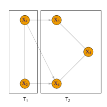
(a)

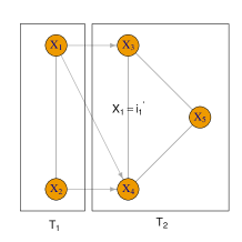
(b)

Figure 1: CG (on the left) and SCG with the stratum $\mathcal{K}^{12}_{34}=\left\{(i_{1}^{\prime},*)\right\}$ (on the right), both with components $T_{1}=\left(1,2\right)$ and $T_{2}=\left(3,4,5\right)$.

Formally, a SCG is defined by three sets, the one of vertices $V$, the one of edges $E$ and the one of stratum $S$ which denotes the labelled arcs. In particular each element of S is a stratum $\mathcal{K}^{C}_{\gamma,\delta}=\left\{i^{\prime}_{C}:\gamma\perp\delta|C=i^{\prime}_{C}\right\}$. which refers to a pair of vertices $(\gamma,\delta)$ and which reports the list of modalities of the veriables in $C$ according to which the arc is missed (and the CS independence holds). Since we are using the SCGM as extension of CGM of type IV, the set $C$, is always included or equal to the set of parents of vertices $(\gamma,\delta)$.

Definition 2.

Given a SCG, the Stratified Markov Properties to extract a list of conditional, marginal and CS independencies are

$$\begin{array}[]{llll}\textsf{C1)}&T_{h}\perp nd(T_{h})|pa_{D}(T_{h}),&h=1,\dots,s;&\\ \textsf{CS2)}&\gamma\perp\delta|pa_{D}(T_{h})=i^{\prime}_{pa_{D}(T_{h})};&i^{\prime}_{pa_{D}(T_{h})}\in\mathcal{K}_{\gamma,\delta}^{pa_{D}(T_{h})}&\text{if}\quad\gamma,\delta\in T_{h};\\ \textsf{CS3)}&\gamma\perp\delta|S_{\gamma,\delta}=pa_{G}(\gamma)=i^{\prime}_{pa_{G}(\gamma)}&i^{\prime}_{pa_{G}(\gamma)}\in\mathcal{K}_{\gamma,\delta}^{pa_{G}(\gamma)}&\text{if}\quad\gamma\in T_{h},\delta\in pa_{D}(T_{h})\backslash pa_{G}(\gamma)\\ \end{array}$$ (11)

where the C1) is equal to the rule C1) in formula (10) and CS2) and CS3) are a generalization of the remaining rules in formula (10).

When in the conditional set of both CS2) and CS3), the stratum $\mathcal{K}_{\gamma,\delta}^{C}$ coincide with $\mathcal{I}_{C}$, we are handling with a conditional indpendence and the stratum is unnecessary. In this case we bring back to the “pairwise” Markov properties for a CGM of type IV as listed in formula (2) of Marchetti & Lupparelli, (2011) that are equivalent to the ones in formula (10).
Graphically, a stratum can be an undirected labelled arc the case of (CS2), or a directed labelled arc, the case pf CS3. However, not any possible stratum is admitted in the SCG model. Let us consider, for instance, the graph in Figure 2, we have the conditional independence $3\perp 2|1$ but, at the same time we have the CS independence $3\perp 1|2=i_{2}^{\prime}$. In the conditional independence we declare that the variable $2$ does not affect variable $3$ for any modality of $1$ but, in the CS independence we affirm that the variable $2$ discriminates the relationship between $1$ and $3$, thus it has some effect on the variable $3$. Nyman et al., (2016) dealt with this situation and, in their Theorem 2, they give the condition for the existence of a stratum that is summarized in the following remark.

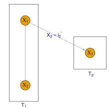
Figure 2: SCG with components $T_{1}=\left(1,2\right)$ and $T_{2}=\left(3\right)$ with a non representable stratum.

Remark 4.

Given a SCG, with at least one stratum $\mathcal{K}_{\gamma,\delta}^{C}\not\equiv\mathcal{I}_{C}$, then the variables in $S$ must be adjacent or parents of both $\gamma$ and $\delta$.

Example 3.3.

(continuation of example 3.2) In Figure 1 (b), we have the stratum $\mathcal{K}^{12}_{34}=\left\{(i_{1}^{\prime},*)\right\}$. Thus, by applying the CS2), the statement $3\perp 4|12=(i_{1}^{\prime},*)$ comes. Note that, the variable $1$ involved by the stratum belongs to both $pa_{G}(3)$ and $pa_{G}(4)$ and the previous remark 4 holds.

4 Regression model with context specific independencies

In Section 2 the main results about the HMM parametrization are discussed, while in Section 3 a graphical model for different kind of independencies is presented. In this section we connect these two models and we show how we can parametrize a SCGM through a HMMM.
As mentioned in Section 3, the approach of CGMs seems natural to explain the effect of some variables (covariates) on a set of dependence variables that can be in turn covariates for other dependence variables. Thus, it is appropriate to collect the variables in the components according to this purpose and, by focusing on each component $T_{h}$, we consider as covariates of $T_{h}$ the variables in $pa_{D}(T_{h})$. The CGM of type IV admits to simplify the regression statements by using a marginal approach for the variables in the same components, as it is shown by Marchetti & Lupparelli, (2011). Here we want to improve this multivariate regression model based on SCGMs by considering ordinal variables coded by local logits and then by simplifying the regression equations thanks to the CS independencies. As it is shown in Marchetti & Lupparelli, (2008), Rudas et al., (2010) and Nicolussi, (2013) the CGM of type IV can be parametrized by using the HMMMs with the appropriate hierarchical marginal sets $\mathcal{H}=\left\{\mathcal{H}_{1},\mathcal{H}_{2}\right\}$ where

$$\begin{array}[]{ll}\mathcal{H}_{1}=&\left\{(pa_{D}(T_{h})\cup A),\,h=1,\dots,s;\,A\subseteq T_{h}\right\}\\ \mathcal{H}_{2}=&\left\{(nd(T_{h})\cup T_{h}),\,h=1,\dots,s\right\}.\end{array}$$ (12)

These two classes must be put together in $\mathcal{H}$ so that if $j<i$ then $\mathcal{M}_{i}\not\subseteq\mathcal{M}_{j}$. Then, focusing on each group of dependent variables, we define the HMM parameters (2) evaluated in each conditional distribution of the covariates. That means, for each set of dependent variables $A\subseteq T_{h}$, we define the parameters $\eta^{A\cup pa_{D}(T_{h})}_{A}(i_{A}|i_{pa_{D}(T_{h})})$ evaluated in any values $i_{pa_{D}(T_{h})}\in\mathcal{I}_{pa_{D}(T_{h})}$ of the covariates $pa_{D}(T_{h})$. All these parameters can be expressed as combination of regression parameters as follows.

Definition 3.

Given a SCGM, regression parameters are given by

$$\eta^{A\cup pa_{D}(T_{h})}_{A}(i_{A}|i_{pa_{D}(T_{h})})=\sum_{t\subseteq pa_{D}(T_{h})}\beta_{t}^{A}(i_{t})\qquad\forall h=1,\dots,s\qquad A\subseteq T_{h}.$$ (13)

Theorem 4.1.

The parameters $\beta_{t}^{A}(i_{t})$ in the regression model (13), are the HMM parameters based on baseline or local logit

$$\beta^{A}_{t}(i_{t})=(-1)^{|pa_{D}(T_{h})\backslash t|}\eta^{(A\cup pa_{D}(T_{h}))}_{tA}(i_{tA}|i^{*}_{pa_{D}(T_{h})\backslash t})$$ (14)

$\forall t\subseteq pa_{D}(T_{h})\neq\emptyset$ and where $i_{tA}=i_{t}\cap i_{A}$.

Example 4.1.

Let us consider the CGM in Figure 1 (a) where there are two components. The first is composed of the purely dependent variables $3$, $5$ and $6$ while in the second there are the covariates $1$ and $2$. Thus, according to the formula (12), the marginal sets take values in $\left\{(123),(124),\right.$ $\left.(125),(1234),(1235),(1245),(12345)\right\}$. By focusing on the dependent variable $4$, we can express the regression model as follows

$$\eta^{123}_{4}(i_{4}|i_{12})=\beta_{\emptyset}^{4}+\beta_{1}(i_{1})^{4}+\beta_{2}^{4}(i_{2})+\beta_{12}^{4}(i_{12})$$

$\forall i_{12}\in\mathcal{I}_{12}$ and $i_{4}\in\left\{1,\dots,I_{4}-1\right\}$ because when $i_{4}=I_{4}$ the parameter is zero by definition. By applying Corollary 2 in Appendix A, we see that the $\beta$ parameters are

$$\begin{array}[]{lll}\beta^{4}_{\emptyset}&=&\eta^{(124)}_{4}(i_{4}|i^{*}_{12})\\ \beta^{4}_{1}(i_{1})&=-&\eta^{(124)}_{14}(i_{14}|i^{*}_{2})\\ \beta^{D}_{2}(i_{2})&=-&\eta^{(124)}_{24}(i_{24}|i^{*}_{1})\\ \beta^{D}_{12}(i_{12})&=&\eta^{(124)}_{124}(i_{124}).\end{array}$$

The parameters in formula (13) are able to explain the relationship between variables in $T_{h}\cup pa_{D}(T_{h})$ for each $h=1,\dots,s$. The remaining relationships between variables belonging to disjointed components can be described by the HMM parameters

$$\eta^{T_{h}\cup nd(T_{h})}_{AB}(i_{AB})$$ (15)

where $h=1,\dots,s$, $A\subseteq T_{h}$ and $B\subseteq nd(T_{h})$ such that $B\cap(nd(T_{h})\backslash pa_{D}(T_{h})\neq\emptyset$.

Theorem 4.2.

The regression parameters in formula (13) and the HMM parameters in formula (15) are a 1:1 function (a reparametrization) of the HMM parameters $\eta_{\mathcal{L}}^{\mathcal{M}}$, $\forall\mathcal{L}\in\mathcal{P}(\mathcal{Q})$ and $\forall\mathcal{M}\in\mathcal{H}$.

Now let us to consider the SCGM as presented in Section 3. The previous considerations about the parametrization still holds and the following theorem explains how to constrain the HMM parameters according to the SGCM.

Theorem 4.3.

A SCGM that obeys to the Stratified Markov Properties of type IV in (11) can be parametrized as follows:

• Each (C1) holds iif the HMM parameters in formula (15) are equal to zero;
  

• Each (CS2) holds iif the regression parameters in formula (13) satisfy $\eta^{\mathcal{L}\cup pa_{D}(T_{h})}_{\mathcal{L}}(i_{\mathcal{L}}|i^{\prime}_{pa_{D}(T_{h})})=0$, $\forall\mathcal{L}$ non connected set such that $(\gamma\cup\delta)\subseteq\mathcal{L}$ when $i^{\prime}_{pa_{D}(T_{h})}\in\mathcal{K}_{\gamma,\delta}^{pa_{D}(T_{h})}$.
  

• Each (CS3) holds iif the regression parameters in formula (13) satisfy $\sum_{t\in C}\beta^{\gamma}_{t}(i^{\prime}_{t})=0$, where $i^{\prime}_{t}=\in\mathcal{K}^{pa_{G}(\gamma)}_{\gamma,\delta}\cap\mathcal{I}_{t}$ .
  

Example 4.2.

Let us consider the CGM in Figure 1 (a) where there are two components. The first is composed of the purely dependent variables $3$, $5$ and $6$ while in the second there are the purely covariates $1$ and $2$. Then the following parameters fully describe the relationships among the 5 variables.

$$\begin{array}[]{lll}\eta^{123}_{3}(i_{3}|i_{12})=&\beta_{\emptyset}^{3}+\beta_{1}(i_{1})^{3},&\forall i_{3}\in\mathcal{I}_{3}-1,\,\forall i_{12}\in\mathcal{I}_{12}\\ &\\ \eta^{123}_{4}(i_{4}|i_{12})=&\beta_{\emptyset}^{4}+\beta_{1}(i_{1})^{4}+\beta_{2}^{4}(i_{2})+\beta_{12}^{4}(i_{12}),&\forall i_{4}\in\mathcal{I}_{4}-1,\,\forall i_{12}\in\mathcal{I}_{12}\\ &\\ \eta^{123}_{4}(i_{4}|i_{12})=&\beta_{\emptyset}^{4},&\forall i_{12}\in\mathcal{I}_{12}\\ &\\ \eta^{123}_{35}(i_{35}|i_{12})=&\beta_{\emptyset}^{35}+\beta_{1}(i_{1})^{35}+\beta_{2}^{5}(i_{2})+\beta_{12}^{35}(i_{12}),&\forall i_{35}\in\mathcal{I}_{35}-1,\,\forall i_{12}\in\mathcal{I}_{12}\\ &\\ \eta^{123}_{45}(i_{45}|i_{12})=&\beta_{\emptyset}^{45}+\beta_{1}(i_{1})^{45}+\beta_{2}^{45}(i_{2})+\beta_{12}^{45}(i_{12}),&\forall i_{45}\in\mathcal{I}_{45}-1,\,\forall i_{12}\in\mathcal{I}_{12}\\ \end{array}$$

5 Application

In this section we study the relationships among a set of variables by using the regression model with CS independences as presented in Section 4. At first we collect the variables in component according to their nature and the possible regression model that we want to study.
Several graphical models were tested and in each of them the likelihood ratio test $G^{2}$ is carried out. The $G^{2}$ compares the model under investigation with the saturated (unconstrained) one; under the null hypothesis the $G^{2}$ follows the $\chi^{2}$ distribution with $df$ equal to the difference between the free parameters in the two models. We reject all models with a p-value lower than $0.05$. Among the non rejected models, we choose the one with greatest Akaike Information Criterion (AIC) and Bayesian Information Criterion (BIC).
Since to testing all possible models, particularly when we handle with CS independencies, is computationally expensive, we implement a three steps procedure to achieve the best SGCM of type IV. At first, we carried out an exploratory phase where we test all CGM with only one missed arc in order to the have an overview of the weakest relationships. Then, we consider as reduced model the CGM without the arcs that have lead to a p-value greater than $0.05$ in the previous step. Starting from the reduced models we add one by one all removed arcs. We choose the CGM with greatest AIC and BIC.
A further simplification of the CGM is obtained evaluating the model with the highest order parameters constrained to zero.
Finally, once obtained the best CGM we move on to further simplification by testing the CS independencies by simplifying the conditional ones that have lead to reject the model.

5.1 Innovation Study Survey 2010-2012

In this section we apply the proposed model on a real dataset. Our aim is to build a chain regression model that study the effect of the innovation in some aspects of the enterprise’s life on the revenue growth without omitting the main features of the enterprise. Thus, we collect the following variables from the survey on the innovation status of small and medium Italian enterprises during the $2010-2012$ ISTAT, (2015). At first, as pure response we consider the revenue growth variable in 2012, GROW (Yes, No) henceforth denoted as variable 1. Then, as mixed variables, we take into account the innovation through three dichotomous variables referring to the period 2009-2012: innovation in products or services or production line or investment in R&D, IPR (Yes, No), innovation in organization system, IOR (Yes, No) and innovation in marketing strategies, IMAR (Yes, No), henceforth denoted as variables 2, 3 and 4, respectively. Finally, the role of purely covariates is entrusted to variables concerning the firm’s featuring in 2009-2012: the main market (in revenue terms), MRKT (A= Regional, B= National, C= International), the percentage of graduate employers, DEG (1= $0\%\vdash 10\%$, 2= $10\%\vdash 50\%$, 3=$50\%\vdash 100\%$) and the enterprise size, DIM (1= Small, 2= Medium), henceforth denoted as variables 5, 6 and 7, respectively. The survey covers $18697$ firms, collected in a $2\times 2\times 2\times 2\times 3\times 3\times 2$ contingency table.
In order to analyse this dataset, we build a chain graph with three components according to the nature of the variables, so in the first component we collect the firm’s features variables (5,6,7), in the second component the innovations variables (2,3,4) and in the third component the revenue growth variabl (1).
In the explanatory phases, we tested the independencies associated to all CGM of type IV with only one missed arc on the HMMM associated. Thus, according to the formula (12), we considered the following marginal sets $\left\{(5,6,7);\,(2,5,6,7);\,(3,5,6,7);\,(4,5,6,7);\,(2,3,5,6,7);\,(2,4,5,6,7);\,\right.$ $\left.(3,4,5,6,7);\,(2,3,4,5,6,7);\,(1,2,3,4,5,6,7)\right\}$. The parameters associated to the dichotomous variables were based on the baseline logits, while, the variables with three modalities have been coded with the local logits. We found the three eligible conditional independencies

(a)

$1\perp 2|34567$,

(b)

$1\perp 4|23567$,

(c)

$1\perp 6|23457$.

By testing the combination of these independencies whom results are reported in Table 2, we choose the HMMM characterized by the (b) and (c), reported at the third row in Table 2, since it is the only model with a $p-value>0.05$.

Independencies	Gsq	df	pval	AIC	BIC
(a), (b)	139.74	108	0.02	-220.26	1190.24
(a), (c)	168.57	120	0.00	-167.42	1149.04
(b), (c)	141.34	120	0.09	-194.66	1121.81
(a), (b) ,(c)	180.97	132	0.00	-131.03	1091.40

Table 2: HMMM which combining the three independencies (a) $1\perp 2|34567$, (b)$1\perp 4|23567$ and (c) $1\perp 6|23457$.

However, from the explanatory phases, there are some clues that independencies between variables $1$ and $2$ could be. Thus, among the (b) and (c), we took into account also the independence (a) and we test all possible CS independencies originated from this last. The preferred model is described by the conditional independencies (b) and (c) and by the CS independence $1\perp 2|34567=(1,*,3,*,1)$ that is when there are no innovation in IORG, when the innovation IMAR assume any modality, when the firm works in an international market, when the percentage of degree employers is whatever and when the firm is small. In correspondence of this model we have df=121, Gsq=141.83, p-val=0.09, AIC=-192.17, BIC=1116.46.
The SCGM associated to this model is displayed in Figure 3. Note that, in the stratum, the conditioning variables $3$ and $5$ are not set to a specific modality because they do not satisfy the condition for a CS independence as summarized in the Remark 4.

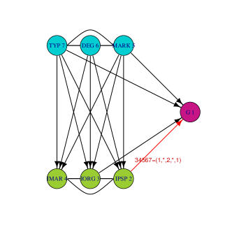
Figure 3: SCGM of type IV with components $T_{1}=(5,6,7)$, $T_{2}=(2,3,4)$ and $T_{3}=(1)$.

By looking at the SCGM in Figure 3 as a regression chain model we can distinguish two regression structures, the first with the dependent variable G with all the others like covariates and the second with the innovation variables as dependent and the featuring variables as covariates. The regression parameters of the two regression models are in Tables 3 and 4 respectively. In particular, in Table 3 we have the regression parameters of the only dependent variable $1$, thus the parameters are logarithms of logits concerning the variable $1$ (probability of no revenue growth against probability on revenue growth) evaluated in all the possible conditioning distributions. Generally speaking, when the parameters in Table 3 are less than zero it means that in the fitted probability having a revenue growth is greater than the probability to have not. In Table 3, the conditional distributions where the difference between the two probabilities achieve high values (greater than 10 in absolute value) are highlight in bold. The cells where this disparity assume huge dimension in negative are where the conditioning distribution of the variables $3,4,5,6,7$ assume value equal to $(1,2,1,2,2,1)$ or $(1,1,1,2,2,1)$, on the other hand, the great disparity in positive is in the cells $(1,1,1,2,1,1)$ and $(1,1,1,1,1,1)$.

$i^{*}_{34567}$	$\eta^{\mathcal{M}}_{1}$	$i^{*}_{34567}$	$\eta^{\mathcal{M}}_{1}$	$i^{*}_{34567}$	$\eta^{\mathcal{M}}_{1}$	$i^{*}_{34567}$	$\eta^{\mathcal{M}}_{1}$
222332	-0,4796	221222	-2,4468	222331	-0,3584	221221	-10,841
122332	-0,4483	121222	-11,5921	122331	-0,3141	121221	-32,7425
212332	-0,1707	211222	-2,071	212331	0,8602	211221	-4,9049
112332	0,6803	111222	-10,9506	112331	3,0365	111221	-27,4244
221332	-0,7988	222122	0,4845	221331	-1,8311	222121	-0,1683
121332	-2,102	122122	1,8001	121331	-3,9632	122121	-2,3828
211332	-0,5672	212122	0,3546	211331	0,1332	212121	0,7241
111332	-1,8448	112122	3,435	111331	0,6237	112121	0,2428
222232	-0,7417	221122	-1,4924	222231	-0,7225	221121	-9,1679
122232	-1,0322	121122	-2,4818	122231	-1,3533	121121	-16,5698
212232	0,8408	211122	-4,8401	212231	3,7374	211121	-11,2031
112232	3,7735	111122	-5,8998	112231	9,8352	111121	-14,355
221232	-1,6234	222312	-0,4355	221231	-3,7989	222311	-0,3504
121232	-5,3967	122312	-0,6114	121231	-9,8567	122311	-0,2496
211232	0,6047	212312	-0,2184	211231	4,2275	212311	1,2512
111232	-0,7702	112312	0,5931	111231	7,1064	112311	5,1493
222132	0,0546	221312	-1,3541	222131	0,7491	221311	-3,6898
122132	1,3823	121312	-4,2052	122131	2,9369	121311	-7,1286
212132	1,0984	211312	-1,3974	212131	3,4766	211311	-0,3392
112132	4,7429	111312	-4,6389	112131	11,8076	111311	2,7044
221132	-0,8322	222212	-0,5193	221131	-2,8954	222211	-0,2307
121132	-0,1691	122212	-0,156	121131	-1,3416	122211	1,8533
211132	-0,5679	212212	1,1386	211131	-0,1813	212211	6,581
111132	2,3733	112212	5,9737	111131	12,1091	112211	22,5741
222322	-0,2048	221212	-2,3837	222321	-0,5180	221211	-6,0503
122322	-0,7378	121212	-6,7821	122321	-3,719	121211	-9,1221
212322	-0,4051	211212	-0,4052	212321	-0,0053	211211	7,674
112322	-0,5112	111212	-0,7885	112321	-4,0535	111211	29,7031
221322	-0,9409	222112	0,5425	221321	-4,3148	222111	1,0062
121322	-4,5919	122112	2,4386	121321	-13,8434	122111	4,9567
211322	-2,1517	212112	1,6583	211321	-4,0426	212111	4,3403
111322	-7,5744	112112	7,265	111321	-16,6193	112111	20,1193
222222	-0,4359	221112	-1,6496	222221	-2,1184	221111	-6,8449
122222	-2,3083	121112	-1,1323	122221	-10,308	121111	-2,5094
212222	0,6317	211112	-2,2924	212221	1,4343	211111	-3,1236
112222	2,0696	111112	2,6188	112221	-5,3214	111111	26,1675

Table 3: Regression parameters concerning the dependent variable 1 with covariates $2,3,4,5,6,7$. The $i^{*}_{34567}$ in table refers to the conditional distribution where the parameters concerning the dependent variable $1$ is evaluated as in formula (13), i.e. $\eta^{\mathcal{V}}_{1}(i_{1}=2|i^{*}_{234567})$ where $V=123456$.

In Table 4 we report the regression parameters concerning the combination of the three dependent variables $2$, $3$ and $4$. In particular, from the 2th to the 4th column there are the parameters associated to the single variables, thus the parameters are logarithms of logits. In the columns 5 to 7 there are the logarithms of contrasts of logists and in the last column there are the third order parameters associated to the variables $2,3,4$. In the first group of columns there is a prevalence of positive parameters which highlight a trend where the probability to make any innovation is lower than the probability to do not, wherever the conditioning distribution is. In the column 5 to 7 there are the pairwise comparison between the different kinds of innovation. Where the parameters are negative, such as in the 4th and in the 6th columns, the probability of concordance between the two innovations considered (i.e. innovation in both aspects or no innovation in both aspects) is lower than the probability of discordance. The opposite case occurs in the 5th column.

$i^{*}_{567}$	$\eta_{2}^{2567}$	$\eta_{3}^{3567}$	$\eta_{4}^{4567}$	$\eta_{23}^{23567}$	$\eta_{24}^{24567}$	$\eta_{34}^{34567}$	$\eta_{234}^{234567}$
332	0,6831	0,5360	-0,1749	-1,7706	-1,9050	-1,5165	0,9079
232	0,6275	0,5631	-0,0295	-1,8384	-1,3781	-1,7466	0,6467
132	0,2105	0,5281	-0,0161	-1,8344	-1,0737	-1,7653	0,4587
322	1,2485	0,6050	-0,0662	-1,9450	-1,2532	-1,5024	-1,1644
222	1,6045	0,6567	0,0426	-2,0638	0,3596	-2,0162	-2,8816
122	1,3508	0,7910	0,3162	-1,9630	0,6518	-1,5455	-3,1860
312	0,7214	-0,0583	-0,4054	-1,8619	-1,8553	-1,5649	-0,5257
212	1,3267	0,3062	0,1200	-1,9385	-0,8871	-1,5361	-1,4836
112	1,0679	0,3998	0,4696	-1,8852	-0,2482	-1,5967	-1,4493
331	0,3001	0,1707	-0,0851	-1,3967	-0,9175	-1,7610	-1,6513
231	0,2883	0,3485	0,5260	-1,7401	0,8988	-2,2774	-3,8131
131	0,3271	0,7048	0,7575	-0,8155	1,2579	-2,0448	-4,1997
321	1,5258	0,7076	0,2295	-1,5524	0,7126	-2,2999	-7,6228
221	2,1658	1,0819	1,0864	-2,2763	4,9992	-3,9665	-15,2039
121	2,8376	1,8068	1,4223	-0,7067	5,1590	-2,7446	-15,6388
311	1,0988	0,0431	0,0358	-1,4920	0,2885	-2,0071	-5,4161
211	2,6186	1,1211	1,1570	-2,0384	3,9245	-2,2946	-10,4366
111	2,8229	1,7590	2,2578	-0,6703	4,7713	-2,1910	-10,4318

Table 4: Regression parameters concerning the dependent variables $2,3,4$ with covariates $5,6,7$.The $i^{*}_{567}$ in table refers to the conditional distribution where the parameters concerning the dependent variables $2,3,4$ is evaluated as in formula (13), i.e. $\eta^{\mathcal{M}}_{1}(i_{1}=2|i^{*}_{567})$.

In conclusion, the output of this application shows a little aspects of the things that we can derive from the application of this models. For instance, once fitted the model it can be used to forecast the values of some dependent variables given the covariate, or again, looking the regression parameters it is possible to define a strategy where to invest. The possibility are several, it depends on the aim of the analysis, the HMMM parameters (that are not listed here) can be used to study the relationships among the variables.

6 Conclusions

In this work we provide several results in the environment of context-specific independences. At first, we focus on the problem to handle with ordinal variables where it is more useful to use parameters based on the local or continuation logits compares to the classical ones based on the baseline logits. In this case, not only we confirm the results on baseline logits such as provided in Nyman et al., (2016), even if in the marginal models, but we provide the results in the case of local and continuation parameters.
Further, we focus on the problem of the graphical representation. We take advantage from the well known relationships between the HMMM and the chain graphical models, in particular the type IV, and we extend the so-called stratified graph to this case.
Finally, we provide the advantage of the use of CS independencies in the Chain Regression models, Marchetti & Lupparelli, (2011) where the CS independencies can simplify the models.
The application shows a small part of the potentiality of this work.

Appendices

A Proofs and further results

Lemma 1.

Given a HMM parameter $\eta_{\mathcal{L}C}^{\mathcal{M}}(i_{\mathcal{L}C})$, where the set $\mathcal{L}C$ is the union of two sets of variables belonging in $\mathcal{M}$, it can be decomposed as follow

$$\eta_{\mathcal{L}C}^{\mathcal{M}}(i_{\mathcal{L}C})=\sum_{\begin{subarray}{c}J\subseteq C\\ J\neq\emptyset\end{subarray}}(-1)^{|J|+1}\eta_{\mathcal{L}(C\backslash J)}^{\mathcal{M}}(i_{\mathcal{L}(C\backslash J)}|i^{*}_{J})+(-1)^{|C|}\eta_{\mathcal{L}}^{\mathcal{M}}(i_{\mathcal{L}}|i_{C})$$ (16)

Proof of Lemma 1

From Proposition (1) of Bartolucci et al., (2007) any parameter $\eta_{\mathcal{L}C}^{\mathcal{M}}(i_{\mathcal{L}C})$ can be rewritten as

$$\eta_{\mathcal{L}C}^{\mathcal{M}}(i_{\mathcal{L}C})=\sum_{J\subseteq C}(-1)^{|C\backslash J|}\eta^{\mathcal{M}}_{\mathcal{L}}(i_{\mathcal{L}}|i_{C\backslash J}i^{*}_{J})$$ (17)

where $\eta^{\mathcal{M}}_{\mathcal{L}}(i_{\mathcal{L}}|i_{C\backslash J}i^{*}_{J})$ is the HMM parameter $\eta^{\mathcal{M}}_{\mathcal{L}}$ evaluated in the conditional distribution where the variables in $C\backslash J$ assume values $i_{C\backslash J}$ and the variables in $J$ are set to a reference modality $i^{*}_{J}$.
When the set $C$ is only one variable, $C=\gamma_{1}$, the decomposition in formula (17) becomes

$$\eta^{\mathcal{M}}_{\mathcal{L}C}(i_{\mathcal{L}C})=\eta^{\mathcal{M}}_{\mathcal{L}}(i_{\mathcal{L}}|i^{*}_{\gamma_{1}})-\eta^{\mathcal{M}}_{\mathcal{L}}(i_{\mathcal{L}}|i_{\gamma_{1}})$$ (18)

that corresponds to formula (16).
When two variables belong to the set $C$, $C=\left\{\gamma_{1},\gamma_{2}\right\}$, by applying the formula (17) only to $\gamma_{1}$ we get

$$\eta^{\mathcal{M}}_{\mathcal{L}C}(i_{\mathcal{L}C})=\eta^{\mathcal{M}}_{\mathcal{L}\gamma_{2}}(i_{\mathcal{L}\gamma_{2}}|i^{*}_{\gamma_{1}})-\eta^{\mathcal{M}}_{\mathcal{L}\gamma_{2}}(i_{\mathcal{L}\gamma_{2}}|i_{\gamma_{1}});$$ (19)

the second addend on the right hand side, can be further decomposed by using the (17) as:

$$\eta^{\mathcal{M}}_{\mathcal{L}\gamma_{2}}(i_{\mathcal{L}\gamma_{2}}|i_{\gamma_{1}})=\eta^{\mathcal{M}}_{\mathcal{L}}(i_{\mathcal{L}}|i_{\gamma_{1}}i^{*}_{\gamma_{2}})-\eta^{\mathcal{M}}_{\mathcal{L}}(i_{\mathcal{L}}|i_{\gamma_{1}\gamma_{2}}).$$ (20)

Now, by considering the HMM parameter $\eta^{\mathcal{M}}_{\mathcal{L}\gamma_{1}}(i_{\mathcal{L}\gamma_{1}}|i^{*}_{\gamma_{2}})$ and by applying the formula (17), we get

$$\eta^{\mathcal{M}}_{\mathcal{L}\gamma_{1}}(i_{\mathcal{L}\gamma_{1}}|i^{*}_{\gamma_{2}})=\eta^{\mathcal{M}}_{\mathcal{L}}(i_{\mathcal{L}}|i^{*}_{\gamma_{1}\gamma_{2}})-\eta^{\mathcal{M}}_{\mathcal{L}}(i_{\mathcal{L}}|i_{\gamma_{1}}i^{*}_{\gamma_{2}}).$$ (21)

Note that the last addend on the right hand side of the (21) is exactly the first addend on the right hand side of (20). Thus, by replacing the (20) and (21) in the (19) we get:

$$\eta^{\mathcal{M}}_{\mathcal{L}C}(i_{\mathcal{L}C})=\eta^{\mathcal{M}}_{\mathcal{L}\gamma_{2}}(i_{\mathcal{L}\gamma_{2}}|i^{*}_{\gamma_{1}})-\eta^{\mathcal{M}}_{\mathcal{L}}(i_{\mathcal{L}}|i^{*}_{\gamma_{1}\gamma_{2}})+\eta^{\mathcal{M}}_{\mathcal{L}\gamma_{1}}(i_{\mathcal{L}\gamma_{1}}|i^{*}_{\gamma_{2}})+\eta^{\mathcal{M}}_{\mathcal{L}}(i_{\mathcal{L}}|i_{\gamma_{1}\gamma_{2}})$$ (22)

that again corresponds to formula (16).
In general, when the set $C$ is composed of $k$ variables, $C=\left\{\gamma_{1},\dots,\gamma_{k}\right\}$, we apply formula (17) recursively, focusing on only one variable of $C$ each time, to any parameter in the formula without any index $i^{*}$ in the conditioning set.

$$\eta^{\mathcal{M}}_{\mathcal{L}C}(i_{\mathcal{L}C})=\sum_{j=1}^{k}(-1)^{j+1}\eta^{\mathcal{M}}_{\mathcal{L}C\backslash(\gamma_{jp}\gamma_{j})}(i_{\mathcal{L}C\backslash(\gamma_{jp}\gamma_{j})}|i^{*}_{\gamma_{j}}i_{\gamma_{jp}})+(-1)^{|C|}\eta_{\mathcal{L}}^{\mathcal{M}}(i_{\mathcal{L}}|i_{C}).$$ (23)

where $\gamma_{jp}=\sum_{i=1}^{j-1}\gamma_{i}$.
Now, we take into account all the parameters having both $i$ and $i^{*}$ in the conditioning set. Let us denote it as $\eta^{\mathcal{M}}_{\mathcal{L}}(i_{\mathcal{L}}|i_{A}i^{*}_{B})$. We can recognise this term in the last term of the right hand side of the decomposition 24 obtained applying the 17 to $\eta^{\mathcal{M}}_{\mathcal{L}A}(i_{\mathcal{L}A}|i^{*}_{B})$:

$$\eta^{\mathcal{M}}_{\mathcal{L}A}(i_{\mathcal{L}A}|i^{*}_{B})=\sum_{\begin{subarray}{c}J\subseteq A\\ J\neq\emptyset\end{subarray}}(-1)^{|A\backslash J|}\eta^{\mathcal{M}}_{\mathcal{L}}(i_{\mathcal{L}}|i^{*}_{BJ}i_{A\backslash J})+\eta^{\mathcal{M}}_{\mathcal{L}}(i_{\mathcal{L}}|i^{*}_{B}i_{A})$$ (24)

By replacing in formula (23) each addend like $\eta^{\mathcal{M}}_{\mathcal{L}}(i_{\mathcal{L}}|i_{A}i^{*}_{B})$ with the expression learned from formula (24), and applying this procedure recursively to any addend like $\eta^{\mathcal{M}}_{\mathcal{L}}(i_{\mathcal{L}}|i_{A}i^{*}_{B})$, we finally obtain exactly the formula 16.

Corollary 2.

A parameter $\eta_{\mathcal{L}}^{\mathcal{M}}$ can be decomposed as the sum of greater order parameters as follows:

$$\eta_{\mathcal{L}}^{\mathcal{M}}(i_{\mathcal{L}}|i_{C})=\sum_{J\subseteq C}(-1)^{|C\backslash J|}\eta_{\mathcal{L}J}^{\mathcal{M}}(i_{\mathcal{L}J}|i^{*}_{C\backslash J})$$ (25)

Proof of Corollary 2

From formula (16), we isolate the last right term having

$$\begin{array}[]{ll}(-1)^{|C|}\eta_{\mathcal{L}}^{\mathcal{M}}(i_{\mathcal{L}}|i_{C})&=\sum_{J\subseteq C}(-1)^{|J|}\eta_{\mathcal{L}(C\backslash J)}^{\mathcal{M}}(i_{\mathcal{L}(C\backslash J)}|i^{*}_{J})\\ \\ \eta_{\mathcal{L}}^{\mathcal{M}}(i_{\mathcal{L}}|i_{C})&=\sum_{J\subseteq C}(-1)^{|C\backslash J|}\eta_{\mathcal{L}(C\backslash J)}^{\mathcal{M}}(i_{\mathcal{L}(C\backslash J)}|i^{*}_{J})\end{array}$$ (26)

By replacing $C\backslash J$ with $J$ in the left side, we get exactly the decomposition in formula (25).

Proof of Theroem 2.1

When the CS independence in formula (3) holds, let us consider the parameters $\eta^{\mathcal{M}}_{\mathcal{L}}$ when $\mathcal{L}=A\cup B\cup C\subseteq\mathcal{M}$. From Lemma 1 we can decompose it as

$$\eta_{ABC}^{\mathcal{M}}(i_{ABC})=\sum_{\begin{subarray}{c}J\subseteq C\\ J\neq\emptyset\end{subarray}}(-1)^{|J+1|}\eta_{AB(C\backslash J)}^{\mathcal{M}}(i_{AB(C\backslash J)}|i^{*}_{J})+(-1)^{|C|}\eta_{AB}^{\mathcal{M}}(i_{AB}|i_{C})$$ (27)

where $\eta^{ABC}_{AB}(i_{AB}|i_{C})$ is the marginal parameter $\eta^{ABC}_{AB}$ evaluated in the conditional distribution $(AB|C=i_{C})$. The term $\eta^{ABC}_{AB}(i_{AB}|i_{C})$ is equal to zero if and only if the CS independence in formula (3) holds. Thus,

$$\begin{array}[]{ll}\eta_{ABC}^{ABC}(i_{ABC})-\sum_{\begin{subarray}{c}J\subseteq C\\ J\neq\emptyset\end{subarray}}(-1)^{|J+1|}\eta_{AB(C\backslash J)}^{ABC}(i_{AB(C\backslash J)}|i^{*}_{J})&=0\\ &\\ \eta_{ABC}^{ABC}(i_{ABC})+\sum_{\begin{subarray}{c}J\subseteq C\\ J\neq\emptyset\end{subarray}}(-1)^{|J|}\eta_{AB(C\backslash J)}^{ABC}(i_{AB(C\backslash J)}|i^{*}_{J})&=0\\ &\\ \sum_{J\subseteq C}(-1)^{|J|}\eta_{AB(C\backslash J)}^{ABC}(i_{AB(C\backslash J)}|i^{*}_{J})&=0\\ &\\ \sum_{c\in\mathcal{P}(C)}(-1)^{|C\backslash c|}\eta_{ABc}^{ABC}(i_{ABc}|i^{*}_{C\backslash c})&=0\\ \end{array}$$ (28)

Note that in the case of baseline coding, the cell $i^{*}_{C\backslash c}$ is equivalent to $i^{**}_{C\backslash c}$ thus the parameters $\eta_{ABc}^{ABC}(i_{ABc}|i^{*}_{C\backslash c})$ is $\eta_{ABc}^{ABC}(i_{ABc})$.
Finally, by considering that the previous decomposition holds for each set $v\in\mathcal{V}=\left\{\left(\mathcal{P}(A)\setminus\emptyset\right)\cup\left(\mathcal{P}(B)\setminus\emptyset\right)\right\}$, the formula (4) comes.

Proof of Theorem 2.2

From the proof of Theorem 2.1, the decomposition in formula (28) still holds. However, by using the local logits $i^{*}_{C\backslash c}\neq i^{**}_{C\backslash c}$ and the identity $\eta^{ABC}_{ABc}(i_{ABc}|i^{*}_{C\backslash c})=\eta^{ABC}_{ABc}(i_{ABc})$ does not hold any more because in local logits $i^{*}_{C\backslash c}$ is equal to $\cap_{j\in C\backslash c}(i_{j}+1)$ while the parameter $\eta^{ABC}_{AB}(i_{AB})$ is built in the conditional distribution where the variables in $C$ assume the reference value $I_{C}$. Note that $\eta^{ABC}_{ABc}(i_{ABc}|i_{C\backslash c}+1)$ does not belong to this parametrization. Now we remark that between the baseline parameters, $\eta_{\textit{b}}$, and the local parameters $\eta_{\textit{l}}$, the following relationship holds:

$$\eta_{\textit{b}\mathcal{L}}^{\mathcal{M}}(i_{\mathcal{L}})=\sum_{i^{\prime}_{\mathcal{L}}\geq i_{\mathcal{L}}}\eta_{\textit{l}\mathcal{L}}^{\mathcal{M}}(i^{\prime}_{\mathcal{L}}).$$ (29)

When the variables in the conditioning set $C$ are based on local logits, it is enough to apply the decomposition in (29) only on the variables in the parameter $\eta_{ABC}^{ABC}(i_{ABC})$ in order to have a baseline approach in $C$. Thus we can rewrite (28) as:

$$\sum_{c\in\mathcal{P}(C)}(-1)^{|C\backslash c|}\sum_{i^{\prime}_{c}\geq i_{c}}\eta_{ABc}^{ABC}(i_{AB}i^{\prime}_{c}|I_{C\backslash c})=0$$ (30)

where $\eta_{ABC}^{ABC}$ are the local parameters and are exactly the same of formula (5). As in proof of the Theorem 2.1, the previous equivalence must hold for each subset $v$ of $A\cup B$ with at least one element in $A$ and one element in $B$.

Proof of Corollary 1

When $i_{C}$ in $\mathcal{K}$ is equal to the last modalities $I_{C}$, for each $c\subseteq C$ and $c\neq\emptyset$, the parameters $\eta^{\mathcal{M}}_{vC}(i_{vC})=0$ by definition, thus formula (5) in Theorem 2.2 becomes $\eta^{\mathcal{M}}_{v}=0$ $\forall v\in\mathcal{V}$. When $\mathcal{K}=\left\{(I_{C\backslash j})\cap(I_{j}-1)\right\}$, that is the modality of every variable is equal to the last but the variable $j$ assumes the modality $I_{j}-1$, the constraints become $\eta^{\mathcal{M}}_{v}(i_{v})=0$ and $\eta^{\mathcal{M}}_{vj}(i_{vj})=0$. Applying this procedure recursively for each $i^{\prime}_{C}$ we obtain the constraints in formula (8).

Proof of Theorem 2.3

For a $c\in\mathcal{P}(C)$ and a $v\in\mathcal{V}$ we consider the parameters $\eta_{vc}^{\mathcal{M}}(i_{vc})$. Note that, each variable $X_{j}$ in $C$ assumes value in $i_{j}$ or in $((i_{j}+1)+\dots+I_{j})$ when it drop in the reference modality. But since in each of these distributions the CS independence (6) holds the parameters are equal to zero.

Proof of Theorem 4.1

By applying formula (25) (Corollary 2) to the HMM parameters in formula (13) evaluated on the conditional distribution $i_{A}|i_{pa_{D}(T_{h})}$ we obtain:

$$\eta^{A\cup pa_{D}(T_{h})}_{A}(i_{A}|i_{pa_{D}(T_{h})})=\sum_{t\subseteq pa_{D}(T_{h})}(-1)^{|t|}\eta^{A\cup pa_{D}(T_{h})}_{tA}(i_{tA}|i^{*}_{pa_{D}(T_{h})\backslash t}).$$ (31)

Thus, the $\beta$ parameters correspond to the addends on the left side of (15).

Proof of Theorem 4.2

When $i_{pa_{D}(T_{h})}=I_{pa_{D}(T_{h})}$, each variable in $pa_{D}(T_{h})$ assumes the last modality, the formula (13) becomes

$$\eta^{A\cup pa_{D}(T_{h})}_{A}(i_{A}|I_{pa_{D}(T_{h})})=\beta_{\emptyset}^{A}=\eta^{A\cup pa_{D}(T_{h})}_{A}(i_{A}).$$ (32)

Now, by considering only one variable $X_{j}\in pa_{D}(T_{h})$ with $i_{j}\neq I_{j}$ and the remaining $pa_{D}(T_{h})\backslash X_{j}$ setting equal to $I_{pa_{D}(T_{h})\backslash X_{j}}$, we have

$$\eta^{A\cup pa_{D}(T_{h})}_{A}(i_{A}|i_{pa_{D}(T_{h})})=\beta_{\emptyset}^{A}+\beta_{j}^{A}(i_{j})=\eta^{A\cup pa_{D}(T_{h})}_{A}(i_{A})-\eta^{A\cup pa_{D}(T_{h})}_{Aj}(i_{Aj})$$ (33)

where we can isolate the term $\eta^{A\cup pa_{D}(T_{h})}_{Aj}(i_{Aj})$. In analogous way we can obtain all HMM parameters defined on $T_{h}\cup pa_{D}(T_{h})$ for each $h=1,\dots,s$. The other parameters are exactly listed in formula (15).

Proof of Theorem 4.3

Let us remember that, given an independence like $A\perp B|C$, the probability distribution of $ABC$ obeys to the independence if and only if the HMM parameters $\eta_{abc}^{\mathcal{M}}=0$ where $a\subseteq A$, $b\subseteq B$, $c\subseteq C$ and $a,b\neq\emptyset$.
Point i). All the HMM parameters in formula (15) refer to the non connected sets of variables involved in formula (C1) of the Markov Properties in (11), thus they are equal to zero.
Point ii). In this case the variables $\gamma$ and $\delta$ belong both to the same component $T_{h}$. Let us focusing on the parameters ground on the baseline logits. Thus, by representing the constraints in (CS2) in formula (11), through the constraints in formula (4), we get becomes $\sum_{t\subseteq pa_{D}(T_{h})}(-1)^{|pa_{D}(T_{h})\backslash t|}\eta_{\gamma\delta t}^{\mathcal{M}}(i_{\gamma\delta}i^{\prime}_{t})$ where the marginal distribution is $\mathcal{M}=\gamma\cup\delta\cup pa_{D}(T_{h})$, $i_{\gamma\delta}=i_{\gamma}\cap i_{\delta}$ and $i^{\prime}_{t}\in\mathcal{K}_{\gamma,\delta}^{pa_{D}(T_{h})}\cap\mathcal{I}_{t}$. By using the equivalence in formula (14) and remembering that in the case of baseline logits the index $i^{*}$ is equal to the index $i^{**}$, we obtain $\sum_{t\in\subseteq pa_{D}(T_{h})}\beta^{\gamma\delta}_{t}(i^{\prime}_{t})=0$. Thus, according to formula (13), we have $\eta_{\gamma\delta}^{\mathcal{M}}(i_{\gamma\delta}|i^{\prime}_{pa_{D}(T_{h})})=0$, $\forall i_{pa_{D}(T_{h})}\in\mathcal{K}_{\gamma,\delta}^{pa_{D}(T_{h})}$.
On the other hand, by considering the parameters based on the local logits, we use the constraints in formula (5) that with (CS2) becomes $\sum_{t\subseteq pa_{D}(T_{h})}(-1)^{|pa_{D}(T_{h})\backslash t|}\sum_{i_{t}\geq i^{\prime}_{t}}\eta_{\gamma\delta t}^{\mathcal{M}}(i_{\gamma\delta}i_{t})$ for $i^{\prime}_{t}\in\mathcal{K}_{\gamma,\delta}^{pa_{D}(T_{h})}\cap\mathcal{I}_{t}$ where $\mathcal{M}=\gamma\cup\delta\cup pa_{D}(T_{h})$, as above. But, according to the relationship between local and baseline parameters in (29), we can rewrite the previous constrast as $\sum_{t\subseteq pa_{D}(T_{h})}(-1)^{|pa_{D}(T_{h})\backslash t|}\eta_{\gamma\delta t}^{\mathcal{M}}(i_{\gamma\delta t}|i^{*}_{pa_{D}(T_{h})\backslash(\gamma\delta t)})$ for $i_{t}\in\mathcal{K}\cap\mathcal{I}_{t}$. Thus the proof follows the baseline case.
Point iii). The (CS3) in formula (11) concerns the independencies with $\gamma\in T_{h}$ and $\delta\in pa_{D}(T_{h})\backslash pa_{G}(\gamma)$. Let us focusing on the parameters based on baseline logits. The constraints on parameters in formula (4) can be express as $\sum_{t\subseteq P}(-1)^{|P\backslash t|}\eta^{\mathcal{M}}_{\gamma t}(i_{\gamma}i^{\prime}_{t}|i^{*}_{P\backslash t})=0$, where $P=pa_{D}(T_{h})\backslash pa_{G}(\gamma)$, $\mathcal{M}=\gamma\cup pa_{D}(T_{h})$, $\forall i_{\gamma}\in\mathcal{I}_{\gamma}$ and $i^{\prime}_{t}\in\mathcal{K}_{\gamma,\delta}^{pa_{G}(\gamma)}$. Now, considering the relationship between HMM and regression parameters express in formula (14), we get $\sum_{t\in P}\beta^{\gamma}_{t}(i^{\prime}_{t})=0$ $\forall i^{\prime}_{t}\in\mathcal{K}_{\gamma,\delta}^{pa_{G}(\gamma)}\cap\mathcal{I}_{t}$. In the case of local coding we must remember that $\eta^{\gamma T}_{\gamma t}(i_{\gamma t}|i^{**}_{T\backslash t})=\sum_{i^{\prime}_{t}\geq i_{t}}\eta^{\gamma T}_{\gamma t}(i_{\gamma}i^{\prime}_{t}|i^{*}_{T\backslash t})$ as showed in formula (29). Thus the reasoning done for baseline can be generalized to the parameters based on the local logits.

References

• Bartolucci etΒ al., (2007) Bartolucci, Francesco, Colombi, Roberto, & Forcina, Antonio. 2007. An extended class of marginal link functions for modelling contingency tables by equality and inequality constraints. Statistica Sinica, 17, 691–711.
• Bergsma & Rudas, (2002) Bergsma, WicherΒ P, & Rudas, Tamas. 2002. Marginal models for categorical data. Annals of Statistics, 140–159.
• Boutilier etΒ al., (1996) Boutilier, Craig, Friedman, Nir, Goldszmidt, Moises, & Koller, Daphne. 1996. Context-specific independence in Bayesian networks. Pages 115–123 of: Proceedings of the twelfth international conference on uncertainty in artificial intelligence. Morgan Kaufmann Publishers Inc.
• Cazzaro & Colombi, (2014) Cazzaro, Manuela, & Colombi, Roberto. 2014. Marginal nested interactions for contingency tables. Communications in Statistics-Theory and Methods, 43(13), 2799–2814.
• Drton, (2009) Drton, Mathias. 2009. Discrete chain graph models. Bernoulli, 736–753.
• Glonek & McCullagh, (1995) Glonek, GariqueΒ FV, & McCullagh, Peter. 1995. Multivariate logistic models. Journal of the Royal Statistical Society. Series B (Methodological), 533–546.
• HΓΈjsgaard, (2004) HΓΈjsgaard, SΓΈren. 2004. Statistical inference in context specific interaction models for contingency tables. Scandinavian Journal of Statistics, 31(1), 143–158.
• ISTAT, (2015) ISTAT. 2015. Italian innovation Survey 2002-2012.
• Lauritzen, (1996) Lauritzen, SteffenΒ L. 1996. Graphical models. Vol. 17. Clarendon Press.
• Marchetti & Lupparelli, (2008) Marchetti, GiovanniΒ M, & Lupparelli, Monia. 2008. Parameterization and fitting of a class of discrete graphical models. COMPSTAT 2008, 117–128.
• Marchetti & Lupparelli, (2011) Marchetti, GiovanniΒ M, & Lupparelli, Monia. 2011. Chain graph models of multivariate regression type for categorical data. Bernoulli, 17(3), 827–844.
• Nicolussi, (2013) Nicolussi, Federica. 2013. Marginal parameterizations for conditional independence models and graphical models for categorical data. Ph.D. thesis, University of Milan Bicocca.
• Nyman etΒ al., (2016) Nyman, Henrik, Pensar, Johan, Koski, Timo, & Corander, Jukka. 2016. Context-specific independence in graphical log-linear models. Computational Statistics, 31(4), 1493–1512.
• Rudas etΒ al., (2010) Rudas, TamΓ‘s, Bergsma, WicherΒ P, & NΓ©meth, RenΓ‘ta. 2010. Marginal log-linear parameterization of conditional independence models. Biometrika, 97(4), 1006–1012.
• Sadeghi & Wermuth, (2016) Sadeghi, Kayvan, & Wermuth, Nanny. 2016. Pairwise Markov properties for regression graphs. Stat, 5(1), 286–294.
• Sadeghi etΒ al., (2014) Sadeghi, Kayvan, Lauritzen, Steffen, etΒ al. 2014. Markov properties for mixed graphs. Bernoulli, 20(2), 676–696.
• Wermuth & Cox, (2004) Wermuth, Nanny, & Cox, DavidΒ R. 2004. Joint response graphs and separation induced by triangular systems. Journal of the Royal Statistical Society: Series B (Statistical Methodology), 66(3), 687–717.
• Whittaker, (2009) Whittaker, Joe. 2009. Graphical models in applied multivariate statistics. Wiley Publishing.