Numerical investigation of the conditioning for plane wave discontinuous Galerkin methods

Abstract

We present a numerical study to investigate the conditioning of the plane wave discontinuous Galerkin discretization of the Helmholtz problem. We provide empirical evidence that the spectral condition number of the plane wave basis on a single element depends algebraically on the mesh size and the wave number, and exponentially on the number of plane wave directions; we also test its dependence on the element shape. We show that the conditioning of the global system can be improved by orthogonalization of the local basis functions with the modified Gram-Schmidt algorithm, which results in significantly fewer GMRES iterations for solving the discrete problem iteratively.

1 Introduction

For the numerical approximation of the Helmholtz problem, it has been shown that, by using non-polynomial basis functions, it is possible to reduce the pollution effect in finite element approximations. One special class of such methods are Trefftz finite element methods, which use basis functions that are local solutions of the homogeneous problem under consideration. For the Helmholtz problem, a common choice of Trefftz basis functions are plane waves; when used in connection to a discontinuous Galerkin variational framework, they lead to the plane wave discontinuous Galerkin (PWDG) method [2, 3, 4, 7, 8, 9]. Containing information on the oscillatory behaviour of the solutions already in the approximation spaces, PWDG deliver better accuracy than standard polynomial finite element methods, for a comparable number of degrees of freedom. In addition, they involve only evaluation of basis functions on mesh interelement boundaries; hence, they can be easily used in connection with general polytopal meshes. However, it is well known that these basis functions are ill conditioned for small mesh sizes, small wavenumbers and large numbers of plane wave directions [10, 11].

The aim of this paper is to numerically investigate the dependence of the elemental and global condition numbers of the PWDG system matrix on the size and shape of the local (convex) polygonal element, the wavenumber, and the number of plane wave directions in the local approximation spaces.

2 The PWDG method for the Helmholtz problem

Let $\Omega\subset\mathbb{R}^{2}$ be a bounded Lipschitz domain and $k>0$ denote the wavenumber. We consider the homogeneous Helmholtz problem with impedance boundary condition:

$$\begin{split}-\Delta u-k^{2}u&=0\quad\textrm{in }\Omega,\\ \nabla u\cdot\mathbf{n}+iku&=g\quad\textrm{on }\partial\Omega,\end{split}$$ (1)

where $i$ denotes the imaginary unit, $\mathbf{n}$ is the unit outward normal and $g\in L^{2}(\partial\Omega)$ is given. The variational formulation of problem (1) reads as follows: find $u\in H^{1}(\Omega)$ such that

$$\int_{\Omega}(\nabla u\cdot\nabla\bar{v}-k^{2}u\bar{v})dx+ik\int_{\partial\Omega}u\bar{v}\,\mathrm{d}s=\int_{\partial\Omega}g\bar{v}\,\mathrm{d}s\quad\mbox{for all }v\in H^{1}(\Omega).$$ (2)

Problem (2) is well posed by the Fredholm alternative argument [13].

We consider a shape-regular, uniform partition $\mathcal{T}_{h}$ of the domain $\Omega$ into convex polygons $K\in\mathcal{T}_{h}$ of diameter $h$. We define the mesh skeleton $\mathcal{F}_{h}=\cup_{K\in\mathcal{T}_{h}}\partial K$, and denote the interior mesh skeleton by $\mathcal{F}_{h}^{I}=\mathcal{F}_{h}\backslash\partial\Omega$. For an element $K\in\mathcal{T}_{h}$ we define the plane wave space $\mathrm{PW}_{p}(K)$ of degree $p$ as

$$\mathrm{PW}_{p}(K)=\{v\in L^{2}(K)\;:\;v(x)=\sum_{j=1}^{p}\alpha_{j}\exp(ik\mathbf{d}_{j}\cdot(\mathbf{x}-\mathbf{x}_{K})),\alpha_{j}\in\mathbb{C}\},$$

where $\mathbf{x}_{K}$ is the mass center of $K$, and $\mathbf{d}_{j}$, $|\mathbf{d}_{j}|=1$, $j=1,\ldots,p$, are $p$ unique directions. Since, in general, small angles between those directions lead to bad conditioning of the basis, we consider equally spaced directions. The PWDG space is defined as

$$\mathrm{PW}_{p}(\mathcal{T}_{h})=\{v_{hp}\in L^{2}(\Omega)\;:\;v_{hp}|_{K}\in\mathrm{PW}_{p}(K)\quad\mbox{for all }K\in\mathcal{T}_{h}\}.$$

The functions in $\mathrm{PW}_{p}(\mathcal{T}_{h})$ are local solutions of the homogeneous Helmholtz problem; therefore, they exhibit the Trefftz property

$$-\Delta v_{hp}-k^{2}v_{hp}=0\quad\mbox{for all }v_{hp}\in\mathrm{PW}_{p}(K).$$

We assume uniform local resolution, i.e., we employ the same uniformly distributed directions $\mathbf{d}_{j}$, $j=1,\ldots,p$ on each element $K\in\mathcal{T}_{h}$.

We use the standard notation for averages and normal jumps of traces across inter-element boundaries, namely $\{\!\!\{\cdot\}\!\!\}$ and $[\![\cdot]\!]$, respectively, and denote by $\nabla_{h}$ the elementwise application of $\nabla$. Hence, we can formulate the PWDG method as follows [7, 8, 9]: find $u_{hp}\in\mathrm{PW}_{p}(\mathcal{T}_{h})$ such that

$$\mathcal{A}_{h}(u_{hp},v_{hp})=\ell_{h}(v_{hp})\quad\mbox{for all }v_{hp}\in\mathrm{PW}_{p}(\mathcal{T}_{h}),$$ (3)

where

$$\mathcal{A}_{h}(u_{hp},v_{hp}) :=i\left[-\int_{\mathcal{F}_{h}^{I}}\{\!\!\{u\}\!\!\}[\![\nabla_{h}\bar{v}]\!]\,\mathrm{d}s+\int_{\mathcal{F}_{h}^{I}}\{\!\!\{\nabla_{h}u\}\!\!\}\cdot[\![\bar{v}]\!]\,\mathrm{d}s\right.$$

$$\qquad-\frac{1}{2}\int_{\partial\Omega}u\nabla_{h}\bar{v}\cdot\mathbf{n}\,\mathrm{d}s+\left.\frac{1}{2}\int_{\partial\Omega}\nabla_{h}u\cdot\mathbf{n}\bar{v}\,\mathrm{d}s\right]$$

$$\qquad+\frac{1}{2k}\int_{\mathcal{F}_{h}^{I}}[\![\nabla_{h}u]\!][\![\nabla_{h}\bar{v}]\!]\,\mathrm{d}s+\frac{k}{2}\int_{\mathcal{F}_{h}^{I}}[\![u]\!]\cdot[\![\bar{v}]\!]\,\mathrm{d}s$$

$$\qquad+\frac{1}{2k}\int_{\partial\Omega}(\nabla_{h}u\cdot\mathbf{n})(\nabla_{h}\bar{v}\cdot\mathbf{n})\,\mathrm{d}s+\frac{k}{2}\int_{\partial\Omega}u\bar{v}\,\mathrm{d}s,$$

$$\ell_{h}(v) :=\frac{1}{2k}\int_{\partial\Omega}g\nabla_{h}\bar{v}\cdot\mathbf{n}\,\mathrm{d}s-\frac{i}{2}\int_{\partial\Omega}g\bar{v}\,\mathrm{d}s.$$

The PWDG method (3) is unconditionally well-posed and stable [2, 3]. The $h$, $p$ and $hp$ convergence has been studied in [2, 7, 8, 9].

Let $A\in\mathbb{C}^{N_{h}\times N_{h}}$ denote the matrix associated with the sesquilinear form $\mathcal{A}_{h}(\cdot,\cdot)$, and $\mathbf{b}\in\mathbb{C}^{N_{h}}$ the vector associated with the functional $\ell_{h}(\cdot)$, for $N_{h}:=\mbox{dim}(\mathrm{PW}_{p}(\mathcal{T}_{h}))$. Then, the algebraic linear system associated with the PWDG method (3) on the mesh $\mathcal{T}_{h}$ is $A\mathbf{u}=\mathbf{b}$.

3 Conditioning of the plane wave basis

In this section, we investigate numerically the conditioning of the local plane wave basis. In order to do so, we consider the spectral condition number of the local mass matrix $M_{K}\in\mathbb{C}^{p\times p}$ on a single element $K\in\mathcal{T}_{h}$. From [6] we get $M_{K,jj}=|K|$, and

$$M_{K,jl} =\int_{K}e^{ik\mathbf{d}_{j}\cdot(\mathbf{x}-\mathbf{x}_{K})}\overline{e^{ik\mathbf{d}_{l}\cdot(\mathbf{x}-\mathbf{x}_{K})}}\,\mathrm{d}\mathbf{x}$$

$$=-\sum_{F\in\partial K\cap\mathcal{F}_{h}}\frac{ik(\mathbf{d}_{j}-\mathbf{d}_{l})\cdot\mathbf{n}}{k^{2}(\mathbf{d}_{j}-\mathbf{d}_{l})\cdot(\mathbf{d}_{j}-\mathbf{d}_{l})}\int_{F}e^{ik(\mathbf{d}_{j}-\mathbf{d}_{l})\cdot(\mathbf{x}-\mathbf{x}_{K})}\,\mathrm{d}s,$$

for $j\neq l$, $1\leq j,l\leq p$, which can be evaluated in closed form. Note that the entries of $M_{K}$ tend to $|K|$ as $k(\mathbf{d}_{j}-\mathbf{d}_{l})\cdot(\mathbf{x}-\mathbf{x}_{K})$ tends to zero; hence, small values of the element size $h$ and wavenumber $k$, or a small angle between two plane wave directions, lead to ill conditioning.

3.1 Dependence on the shape

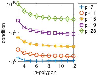
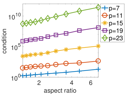
Figure 1: Spectral condition numbers of $M_{K}$ for regular $n$-polygons (left) and anisotropic rectangles (right) with $h=1$ and $k=10$.

The initial numerical experiments investigate the conditioning of the basis for different shapes of the element, for a fixed wavenumber $k=10$.

Firstly, we consider regular $n$-polygons with element size $h=1$; cf. Figure 1 (left). We observe that the condition numbers grow in the number of plane waves directions $p$, but are smaller for larger $n$. In particular, the condition number is decreasing in the number of sides $n$ and is asymptotically stable; hence, small edges do not cause any problems. It has been noted in [11] that the conditioning of the basis depends on the aspect ratio of the elements. Therefore, we consider a single anisotropic rectangle, with size $h=1$, and vary its aspect ratio. We see that the condition number increases exponentially as the aspect ratio increases; cf. Figure 1 (right).

3.2 Dependence on $hk$ and $p$

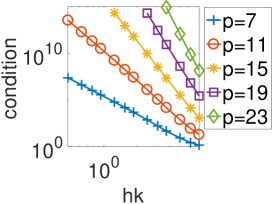
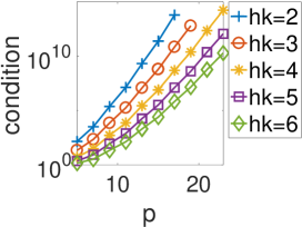
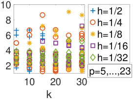
Figure 2: Dependence of the condition number of $M_{k}$ on $hk$ and $p$, and verification of the approximation (4).

In this section we empirically determine the dependence of the condition number on $hk$ and $p$. We restrict to the case of a single square element. The numerical experiments displayed in the first two graphs in Figure 2 suggest that the condition number is algebraic with respect to $hk$ and exponential with respect to $p$. To get a more precise answer, we fitted the data obtained from numerous numerical experiments to

$$\mbox{cond}_{2}(M_{K})\approx\frac{2.34^{p\ln p}}{(hk)^{p-1}}.$$ (4)

In Figure 2 (right) we show the values of $\mbox{cond}_{2}(M_{K})/(\frac{2.34^{p\ln p}}{(hk)^{p-1}})$ for values $h=2^{-1},...,2^{-5}$, $k=5,\ldots,30$ and $p=5,\ldots,23$. To obtain reliable data, we only plot data points for which $\mbox{cond}_{2}(M_{K})<10^{15}$, due to double precision limitations, and for which $hk<10$, due to the resolution condition. Hence, we could only cover a moderate range of values for $h$, $k$ and in particular $p$. All the presented values of $\mbox{cond}_{2}(M_{K})/(\frac{2.34^{p\ln p}}{(hk)^{p-1}})$ are between $1$ and $10$ (recall that the corresponding values of $\mbox{cond}_{2}(M_{K})$ are between $1$ and $10^{15}$), which confirms that the approximation (4) is reasonable, at least for moderate $h$, $k$ and $p$.

4 Orthogonalization of the plane wave basis

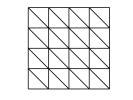
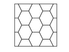
Figure 3: Three different meshes.

In the previous section, we have observed that the condition number of the local basis is large for small $hk$ or large $p$. In this section we aim at improving the conditioning of the local basis in order to lower the condition number of the global system matrix $A$. Therefore, we will investigate the effect of orthogonalization of the (local) basis functions on the conditioning of the (global) system matrix $A$. A different approach has been presented in [10], where improvement of the conditioning of the global system is achieved by suitably designed non-uniform distributions of $p$.

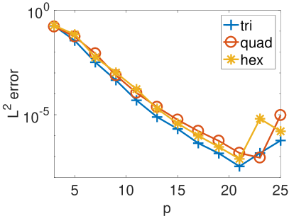
Figure 4: Spectral condition numbers for $k=10$ in double precision arithmetic.

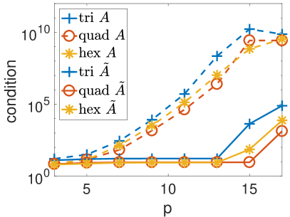
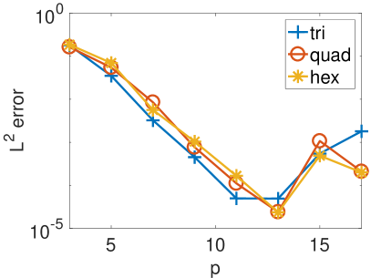
Figure 5: Spectral condition numbers for $k=10$ in single precision arithmetic.

We compare the condition numbers of the system matrix $A$ with original basis functions with that of the system matrix $\widetilde{A}:=Q^{T}AQ$ with orthogonalized basis functions for the three different meshes displayed in Figure 3. Here, $Q\in\mathbb{C}^{N_{h}\times N_{h}}$ denotes the transformation matrix obtained by modified Gram-Schmidt orthogonalization [15] of the (local) basis functions with respect to the Hermitian part of the local system matrix $H(A_{K}):=\frac{A_{K}+\bar{A}_{k}^{T}}{2}$ on each element $K$ separately; cf. [1, 12, 14] for application of modified Gram-Schmidt to partition of unity methods, (polynomial) DG methods, and virtual element methods, respectively. In all experiments, we choose $k=10$ and only investigate the effect on the critical dependence of the condition number on $p$. As a model problem, we consider problem (1) with $\Omega=(0,1)^{2}$, and exact solution given by the Bessel function of the third kind (Hankel function) $u(\mathbf{x})=H^{1}_{0}(k\sqrt{(x_{1}+1/4)^{2}+x_{2}^{2}})$.

In Figure 4 (left), we observe, for all meshes, the expected increase of the condition number in $p$ for the original system matrix $A$ (dashed lines), which results in the loss of accuracy in the $L^{2}$ error for $p>21$, cf. Figure 4 (right), when using a direct linear solver. We observe major improvements of the condition numbers for the matrix $\widetilde{A}$ (solid lines) until $p=21$ when the (modified) Gram-Schmidt orthogonalization breaks down, which directly correlates to the point when the direct solver fails to produce a more accurate solution. Note that, for the original matrix $A$, there is no such correlation. To further investigate these results, we also carried out the same experiments in single precision arithmetic. Figure 5 shows the results for single precision, where we observe that the loss of accuracy already occurs at $p=13$. Note, again, that this loss is correlated to the failure of the orthogonalization, indicated by the sudden increase of the condition numbers for $\widetilde{A}$ at $p=13$.

	$p=5$	$p=7$	$p=9$	$p=11$	$p=13$	$p=15$
$\lambda_{min}(H(A))$	$7.75\cdot 10^{-1}$	$2.56\cdot 10^{-1}$	$1.16\cdot 10^{-2}$	$4.50\cdot 10^{-4}$	$6.73\cdot 10^{-6}$	$1.18\cdot 10^{-7}$
$\lambda_{min}(H(A^{-1}))$	$3.83\cdot 10^{-2}$	$2.70\cdot 10^{-2}$	$2.09\cdot 10^{-2}$	$1.71\cdot 10^{-2}$	$1.44\cdot 10^{-2}$	$1.25\cdot 10^{-2}$
GMRES ($A$)	60	96	135	159	193	217
$\lambda_{min}(H(\widetilde{A}))$	$1.10\cdot 10^{-1}$	$8.45\cdot 10^{-2}$	$8.29\cdot 10^{-2}$	$8.27\cdot 10^{-2}$	$7.44\cdot 10^{-2}$	$6.08\cdot 10^{-2}$
$\lambda_{min}(H(\widetilde{A}^{-1}))$	$5.02\cdot 10^{-1}$	$5.00\cdot 10^{-1}$	$5.00\cdot 10^{-1}$	$5.00\cdot 10^{-1}$	$5.00\cdot 10^{-1}$	$5.00\cdot 10^{-1}$
GMRES ($\widetilde{A}$)	47	52	58	62	68	73

Table 1: Eigenvalue approximations and GMRES iteration count for the original basis and the orthogonalized basis using the second mesh of Figure 3 and $k=10$.

Finally, we are interested in the effect of the orthogonalization on the convergence of iterative solvers such as GMRES. From the convergence theory of GMRES [5], provided that $H(A)$, the Hermitian part of the system matrix A, is positive definite, the residual contraction factor, for the residual $r_{j}$ at iteration $j$, can be bounded as

$$\frac{\|r_{j}\|}{\|r_{0}\|}\leq\left(1-\lambda_{min}(H(A))\lambda_{min}(H(A^{-1}))\right)^{j/2}.$$

Therefore, in Table 1, we report $(\lambda_{min}(H(A)),\lambda_{min}(H(A^{-1})))$, for the system matrix $A$ with the original basis, and $(\lambda_{min}(H(\widetilde{A})),\lambda_{min}(H(\widetilde{A}^{-1})))$, for the system matrix $\widetilde{A}$ obtained with the orthogonal basis, along with the number of GMRES iterations needed in order to reduce the residual of a factor $10^{-10}$. We observe that, for increasing $p$, the values $\lambda_{min}(H(A^{-1}))$ and $\lambda_{min}(H(\widetilde{A}^{-1}))$ are fairly constant, while the values $\lambda_{min}(H(A))$ and $\lambda_{min}(H(\widetilde{A}))$ decrease significantly. However, the values of $\lambda_{min}(H(\widetilde{A}))$ decrease much more slowly than those of $\lambda_{min}(H(A))$, which results in a far slower increase of GMRES iterations for the orthogonalized basis than for the original one. As we merely change the basis and do not precondition the system matrix, we cannot expect a constant number of GMRES iterations.

5 Conclusions

We have provided empirical evidence that, in 2D, the condition number of the plane wave basis is stable for large edge counts in regular polygons, and grows as the aspect ratio of the anisotropy of the elements increases. We also observed its algebraic dependence on the product $hk$, and exponential dependence on $p$. It has been demonstrated that the condition number of the global system matrix can be significantly lowered by a local modified Gram-Schmidt orthogonalization with respect to the Hermitian part of the local system matrix; this results in faster convergence of the GMRES solver. The improvement of the conditioning in 3D will be considered in future work.

References

- [1] F. Bassi, L. Botti, A. Colombo, D. A. Di Pietro, and P. Tesini, On the flexibility of agglomeration based physical space discontinuous Galerkin discretizations, J. Comput. Phys. 231:1 (2012), 45–65.
- [2] A. Buffa and P. Monk, Error estimates for the ultra weak variational formulation of the Helmholtz equation, M2AN Math. Model. Numer. Anal. 42:6 (2008), 925–940.
- [3] O. Cessenat and B. Després, Application of an ultra weak variational formulation of elliptic PDEs to the two-dimensional Helmholtz problem, SIAM J. Numer. Anal. 35:1 (1998), 255–299.
- [4] , Using plane waves as base functions for solving time harmonic equations with the ultra weak variational formulation, J. Comput. Acoust. 11:2 (2003), 227–238.
- [5] S. C. Eisenstat, H. C. Elman, and M. H. Schultz, Variational iterative methods for nonsymmetric systems of linear equations, SIAM J. Numer. Anal. 20:2 (1983), 345–357.
- [6] C. Gittelson, Plane wave discontinuous Galerkin methods, Master’s thesis, SAM, ETH Zurich, Switzerland, 2008.
- [7] C. J. Gittelson, R. Hiptmair, and I. Perugia, Plane wave discontinuous Galerkin methods: analysis of the -version, M2AN Math. Model. Numer. Anal. 43:2 (2009), 297–331.
- [8] R. Hiptmair, A. Moiola, and I. Perugia, Plane wave discontinuous Galerkin methods for the 2D Helmholtz equation: analysis of the -version, SIAM J. Numer. Anal. 49:1 (2011), 264–284.
- [9] , Plane wave discontinuous Galerkin methods: exponential convergence of the -version, Found. Comput. Math. 16:3 (2016), 637–675.
- [10] T. Huttunen, P. Monk, and J. P. Kaipio, Computational aspects of the ultra-weak variational formulation, J. Comput. Phys. 182:1 (2002), 27–46.
- [11] T. Luostari, T. Huttunen, and P. Monk, Improvements for the ultra weak variational formulation, Internat. J. Numer. Methods Engrg. 94:6 (2013), 598–624.
- [12] L. Mascotto, Ill-conditioning in the virtual element method: stabilizations and bases, Numer. Methods Partial Differential Equations. 34:4 (2018), 1258–1281.
- [13] J. Melenk, On generalized finite element methods, Ph.D. thesis, University of Maryland, 1995.
- [14] M. A. Schweitzer, Stable enrichment and local preconditioning in the particle-partition of unity method, Numer. Math. 118:1 (2011), 137–170.
- [15] G. W. Stewart, Matrix algorithms. Vol. I: Basic decompositions, Society for Industrial and Applied Mathematics, Philadelphia, PA, 1998.