The strong coupling: a theoretical perspective

Abstract

This contribution to the volume “From My Vast Repertoire — The Legacy of Guido Altarelli” discusses the state of our knowledge of the strong coupling.

CERN-TH-2017-268

1 Introduction

Chapter The strong coupling:
a theoretical perspective

The strong coupling, $\alpha_{s}$, is one of the fundamental parameters of the Standard Model. It enters into all cross section calculations for processes at the Large Hadron Collider (LHC), whether directly at leading order, or through higher-order QCD calculations. It also enters indirectly through the evolution of parton distribution functions (PDFs) and their correlation with the strong coupling. Consequently, as the LHC experiments’ work evolves towards precision physics, accurate knowledge of the strong coupling is becoming increasingly important. The value of the coupling matters also for the question of gauge coupling unification at high scales and for the stability of the universe in any given particle-physics scenario.

The question of the value of $\alpha_{s}$ is hotly debated, with a range of discussions in the literature [1, 2, 3, 4, 5]. It’s a subject that Guido had an active interest in [6]. Since, with Siggi Bethke and Günther Dissertori, I’m one of the authors of the PDG review chapter on QCD, which also includes a discussion and average of $\alpha_{s}$, we often had exchanges on the subject. As I’ll explain below, Guido was rather critical of our PDG approach to the question.

To illustrate the problem of establishing the value of $\alpha_{s}$, consider the two following determinations: one, from a lattice-QCD calculation of Wilson loops, quotes $\alpha_{s}(m_{Z})=0.11840\pm 0.00060$ [7]; another, from a fit to the thrust distribution in $e^{+}e^{-}$ collisions [8], yields $0.1135\pm 0.00105$. The two determinations are four standard deviations apart from each other, and there is no single value of $\alpha_{s}$ that isn’t at least three standard deviations from one or other of them. Both determinations pay extensive attention to the question of potential systematic uncertainties, yet in all likelihood, at least one of the two has underestimated them.

A first question is what accuracy do we need for the strong coupling. Consider the case of LHC phenomenology. The change induced in key LHC cross sections, e.g. the top-quark cross section or the Higgs-boson cross section, in going from $\alpha_{s}=0.118$ to $\alpha_{s}=0.113$ is a reduction of about $8{-}9\%$. This is larger than the total theoretical uncertainties on these cross sections from missing higher-order corrections (about $4-6\%$ [14, 11]) and larger also than current or foreseen experimental uncertainties: the top cross section is measured to about $3-4\%$ uncertainty [15, 16], and in the long term the Higgs cross section should also reach a similar or better precision. Even a $1\%$ uncertainty on $\alpha_{s}$ leads to effects that are comparable to any other single theoretical uncertainty on the Higgs cross section, i.e. at the $2\%$ level. Therefore, only for a determination of the coupling with a precision comfortably below the percent level can $\alpha_{s}$ uncertainties largely be ignored for extracting fundamental information from the LHC.

To understand the limitations that arise in determining the strong coupling, it is useful to keep in mind the essence of any determination of the coupling. Some quantity $V$ is measured experimentally, giving a result $V_{\text{exp}}\pm\delta V_{\text{exp}}$. This needs to be related to a theoretical prediction for the same quantity in terms of powers of the coupling,

$$V_{\text{th}}(\alpha_{s}(\mu),\mu)=\sum_{n}^{N}c_{n}(\mu)\alpha_{s}^{n}(\mu)+{\cal O}\!\left(\alpha_{s}^{N+1}\right)+{\cal O}\!\left(\frac{\Lambda^{p}}{Q^{p}}\right)\,,$$ (1)

where the $c_{n}$ factors are the coefficients of the perturbative series, which can in practice be calculated up to some finite order $n=N$. They depend on the choice of renormalisation scale $\mu$, as does the coupling itself. The quantity $\Lambda$ is the non-perturbative scale of QCD and $Q$ is the order of magnitude of the momentum transfer in the process used for measuring $V$. The term $\frac{\Lambda^{p}}{Q^{p}}$ reflects the inevitable existence of non-perturbative contributions. Our understanding of its structure and relevance is, in some contexts, the subject of debate, though in most cases at the least the value of the power $p$ is known.

Requiring $V_{\text{th}}(\alpha_{s}(\mu),\mu)=V_{\text{exp}}$ in Eq. (1) fixes $\alpha_{s}$. The uncertainty on the $\alpha_{s}(m_{Z})$ determination then has three sources: (i) the extent to which $V$ can be measured precisely, i.e. the size of the $\delta V_{\text{exp}}$ uncertainty; (ii) the estimated impact of terms $c_{n}$ beyond those that can be calculated with today’s technology, of order $\alpha_{s}^{N+1}$, e.g. as found by varying $\mu$; and (iii) the size of the “power correction” terms, $\Lambda^{p}/Q^{p}$ and the degree to which they can be reliably understood. There may also be missing higher-order electroweak terms, or uncertainties associated with other fundamental parameters. The discussion of different determinations will essentially be a discussion of the relative sizes of each of these sources of uncertainty, and the degree of consensus on our understanding of them.

The Particle Data Group (PDG) [5] world average (in the QCD review chapter) limits its inputs to cases where the perturbative series is known at least to next-to-next-to-leading order (NNLO), and in the interests of brevity the discussion below will similarly concentrate on those cases. In the PDG we have taken the approach that we should be as neutral as possible with regard to disputes in the community about different determinations, with uniform prescriptions applied to all reasonable determinations. That is motivated in part by a desire to minimise any risk of bias in the outcome of the average. I think it’s fair to say that Guido wasn’t impressed by this approach. In our discussions on the subject he would insist that one should attempt to bring a theorist’s critical view to each determination. He argued

[…] one should select few theoretically simplest processes for measuring $\alpha_{s}$ and consider all other ways as tests of the theory.

In the chapter I’ll give my take on what is needed to make a “clean” determination of the strong coupling: clean (and “transparent”) were words regularly used by Guido in this context.

2 Jet rates and event shapes and in $e^{+}e^{-}$ collisions

One natural way of thinking about the meaning of the QCD coupling is that it governs the probability of emitting a gluon. Gluons, of course, cannot be directly observed, but jets of hadrons can be used as a stand-in for hard gluons, i.e. for gluons that are energetic and radiated at large angles with respect to their emitter.

The simplest environment in which to study jets is $e^{+}e^{-}\to\text{hadrons}$ reactions. Perturbatively, the lowest order process is $e^{+}e^{-}\to q\bar{q}$, i.e. a two-jet event. There is a probability $\alpha_{s}$ to radiate a hard gluon, giving $e^{+}e^{-}\to q\bar{q}g$, i.e. a three-jet event. By measuring the fraction of three-jet events one can determine $\alpha_{s}$.

There is considerable freedom in how one carries out the extraction: there are different algorithms for defining the jets, including the Durham [18] and Cambridge [19] algorithms. Each algorithm comes with a parameter to define how energetic the emission should be in order to be considered a jet. For the Durham and Cambridge algorithms, the parameter is called $y_{\text{cut}}$, and corresponds to the squared transverse momentum of the emission, normalised to the squared centre-of-mass energy.

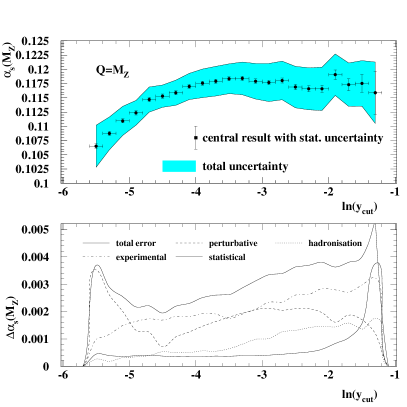
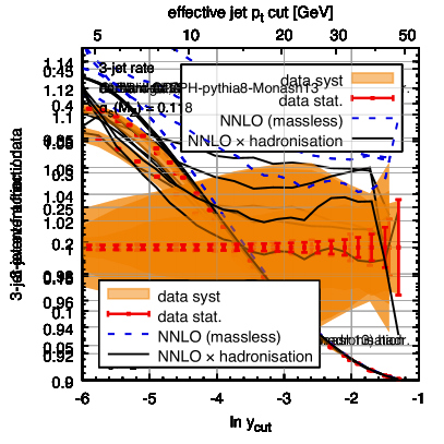
Figure 1: Top left: comparison of ALEPH jet rate data [20] for the Durham algorithm with the pure NNLO result for $\alpha_{s}(m_{Z})=0.118$ [21] (see also [22, 23]), and the NNLO result multiplied by hadronisation corrections estimated with Pythia 6.428 [24] with the DW tune. Top right: strong coupling (top) and the uncertainty breakdown from the ALEPH jet rate extraction (Fig. 1 of Ref. [25]). Bottom left: ratio of NNLO theory to data for $\alpha_{s}(m_{Z})=0.118$, with the same data and simulation choices as for the top-left plot. Bottom right: ratio of NNLO theory to data for $\alpha_{s}(m_{Z})=0.118$, but now with the Cambridge jet algorithm, OPAL data and Pythia 8.223 [26] (Monash 2013 tune [27]) for the hadronisation.

To illustrate some of the characteristics and challenges of extractions of the coupling from jet rates, Fig. 1 (top-left) shows the Durham 3-jet rate as a function of $y_{\text{cut}}$, as measured by the ALEPH collaboration at particle (i.e. hadron) level. It is compared to the pure NNLO prediction in 5-flavour massless QCD at parton level and to the NNLO result multiplied by an additional hadronisation correction. The upper axis shows the effective transverse momentum ($p_{t}$) cut that a given value of $\ln y_{\text{cut}}$ corresponds to. For a typical choice $\ln y_{\text{cut}}=-4.0$, one hovers close to a $p_{t}$ cut of $10\,\text{GeV}$. If one considers that a jet’s energy may change by an amount of the order of a GeV due to the parton to hadron transition, then the fact that the jet $p_{t}$ is just $10\,\text{GeV}$ becomes a concern. That parton-to-hadron transition is believed to be the main reason the NNLO (parton) theory doesn’t immediately agree with the hadron-level data. To extract a value of the coupling it is mandatory to apply a hadronisation correction to the NNLO prediction (and also corrections for $b$-quark mass effects). This was done for the analysis in the top right-hand plot of Fig. 1, using Monte Carlo event generators to estimate the hadronisation correction (about a $5\%$ effect). The plot shows the ALEPH collaboration’s resulting extraction of the strong coupling as a function of $y_{\text{cut}}$ [25]. For $\ln y_{\text{cut}}>-4$ the extracted $\alpha_{s}$ value is fairly independent of $y_{\text{cut}}$, a sign of robustness of the analysis. Below that, however, the result depends substantially on the choice of $y_{\text{cut}}$. One can attribute that feature to a breakdown of fixed-order perturbation theory, associated with logarithmically enhanced terms of the perturbative series, which go as $(\alpha_{s}\ln^{2}y_{\text{cut}})^{n}$.

The final extraction from the ALEPH collaboration involves a choice of $\ln y_{\text{cut}}\simeq-3.9$ that remains within the plateau and minimises the final error. It gives:

$$\alpha_{s}(m_{Z})=0.1175 \pm 0.0004\text{(stat.)}\pm 0.0016\text{(det.)}\pm 0.0011\text{(exp.)}$$

$$\pm 0.0006\text{(had.)}\pm 0.0002\text{(mass)}\pm 0.0014\text{(pert.)}\,,$$

$$=0.1175 \pm 0.0025\text{(total)}\,,$$

for which the dominant quoted error sources are detector and other experimental systematics as well as missing high-order contributions (assessed through variation of the renormalisation scale).

The aspect of this kind of determination that is perhaps most called into question is the hadronisation correction, because the way non-perturbative effects arise in Monte Carlo simulations (through a cutoff) does not match the way they need to be applied to perturbative calculations. Rather than applying a cutoff at some scale of order $1\,\text{GeV}$, perturbative calculations integrate down to zero momentum, but using an integrable, perturbative expansion of the coupling. The overall size of the hadronisation correction is $4-5\%$, as is visible from the ratio plot in the bottom-left of Fig. 1. The definition of how hadronisation interfaces with a perturbative calculation could conceivably modify this by a couple of percent.

A further question with jet-rate data is the stability of the determination. The bottom-right plot of Fig. 1 is analogous to the bottom-left one except that the OPAL data replaces the ALEPH data, the jet algorithm has been switched to the Cambridge algorithm and hadronisation corrections have been evaluated with the Pythia 8 generator instead of Pythia 6. The ratio of theory to data goes up by over $6\%$, with each of the three changes accounting for about one third of that. Since the OPAL data have larger systematic uncertainties than the ALEPH data, the results appear to be still (just barely) compatible with $\alpha_{s}(m_{Z})=0.118$. Nevertheless the difference between the bottom left and right-hand plots of Fig. 1 could be taken as a more conservative estimate of the possible size of theoretical uncertainties in $\alpha_{s}$ determinations from $e^{+}e^{-}$ jet rates.

Table 1: Determinations of the strong coupling from jet rates and event shapes in $e^{+}e^{-}$ collisions.

Determination	Data and procedure	Reference
$0.1175\pm 0.0025$	ALEPH 3-jet rate (NNLO+MChad)	[25]
$0.1199\pm 0.0059$	JADE 3-jet rate (NNLO+NLL+MChad)	[29]
$0.1224\pm 0.0039$	ALEPH event shapes (NNLO+NLL+MChad)	[30]
$0.1172\pm 0.0051$	JADE event shapes (NNLO+NLL+MChad)	[31]
$0.1189\pm 0.0041$	OPAL event shapes (NNLO+NLL+MChad)	[32]
$0.1164\;^{+0.0028}_{-0.0026}$	Thrust (NNLO+NLL+anlhad)	[33]
$0.1134\;^{+0.0031}_{-0.0025}$	Thrust (NNLO+NNLL+anlhad)	[34]
$0.1135\pm 0.0011$	Thrust (SCET NNLO+N3LL+anlhad)	[8]
$0.1123\pm 0.0015$	C-parameter (SCET NNLO+N3LL+anlhad)	[35]

The ALEPH result is reproduced in table 1 together with a range of other strong-coupling determinations (all at least at NNLO) from hadronic final-state measurements at LEP and earlier $e^{+}e^{-}$ colliders. As well as jet rates, they also make use of “event shapes” such as the thrust [36, 37], $C$-parameter [38] or jet broadenings [39]. Each event shape provides a continuous measure of the extent to which an event’s energy flow departs from a pure back-to-back (i.e. leading order $e^{+}e^{-}\to q\bar{q}$) structure. One sees that the central values and uncertainties for $\alpha_{s}$ vary quite substantially between determinations, even though they all relate to the same underlying phenomenon, the probability of gluon emission from a quark-antiquark system. This is perhaps unsurprising given what we’ve seen in Fig. 1.

The result with the highest quoted precision is that for the thrust (SCET),

$$\alpha_{s}(m_{Z})=0.1135\pm 0.0002_{\text{exp.}}\pm 0.0005_{\text{hadr.}}\pm 0.0009_{\text{pert.}}=0.1135\pm 0.0011\,,$$ (2)

closely followed by the C-parameter determination. A first point to be aware of is that in the 2-jet limit the thrust and $C$-parameter are highly correlated, both in the data and in the structure of the theoretical calculations. The two extractions are very similar in approach: they supplement fixed-order perturbation theory with the resummation of enhanced logarithmic contributions, specifically accounting for terms ranging from $\alpha_{s}^{n}\ln^{n+1}$ down to $\alpha_{s}^{n}\ln^{n-2}$, i.e. N³LL accuracy. Furthermore they use an analytic estimate of hadronisation corrections with a fitted free parameter, which to a first approximation corresponds to a shift of the distribution by a shift of the thrust (specifically $1-T$) or $C$-parameter by an amount proportional to a “power correction” $\Lambda/Q$ (see the reviews [40, 41]). An advantage of analytic hadronisation estimates is that they can address the concern of matching Monte Carlo hadronisation corrections to perturbative calculations.

Guido’s comment about the thrust result was

I think that this is a good example of an underestimated error which is obtained within a given machinery without considering the limits of the method itself.

What might these methodological limitations be? One is that the formalism of resummation holds only for $C,1-T\ll 1$, where every emission is so soft and collinear that one can effectively neglect the kinematic cross-talk (e.g. energy-momentum conservation) that arises when there are multiple emissions. There is almost no quantification in the literature of the corrections induced by such cross-talk, so they potentially represent a neglected systematic error.

Another limitation is that the power correction that is used holds in the 2-jet limit, i.e. $1-T\ll 1$. However the fits extend into the full 3-jet region, e.g. $(6\,\text{GeV})/Q<1-T<0.33$ for the thrust, keeping in mind that $1-T=\frac{1}{3}$ is the largest value that can be obtained with 3 partons. One way of viewing the problem is that the power correction in this region should be governed by a different operator and simply taking the 2-jet result is risky. A different way of phrasing this is that if the average effect of hadronisation is essentially a shift of $1-T$ by an amount $\delta\sim\Lambda/Q$, then $\delta$ itself is likely to be a non-trivial function of the parton-level value of $1-T$. Only for small values of $1-T$ may one neglect that functional dependence.

A sign that this might be causing problems comes from the dependence of the thrust fit results on the choice of limits. Fig. 17 of Ref. [8] shows that modestly restricting the fit range to $(8\,\text{GeV})/Q<1-T<0.25$ increases the central fit value to about $0.1151$, an increase of $0.0016$ relative to Eq. (2), which is larger than the overall quoted error of $0.0011$.

Yet another concern relates to the treatment of experimental systematic errors. The ALEPH fit had total detector and experimental systematic errors of $0.0019$, to be compared to those quoted in the SCET thrust fit of $0.0002$. Even if the latter puts together several experimental results, such a large reduction is puzzling.

What do I conclude about event shapes? Ultimately I have doubts about how realistic it is to extract $\alpha_{s}(m_{Z})$ with $1\%$ precision from data whose underlying physical scale is $10{-}20\,\text{GeV}$, using observables that have $\sim 1\,\text{GeV}/Q$ power corrections. Perhaps, today, the value of such fits should instead be seen in terms of what they might teach us about the limits of our understanding of hadronisation corrections and also of resummation.

3 LEP electroweak fits

Rather than looking for the signature of actual gluon emission, electroweak (EW) fits for $\alpha_{s}$ rely on the slight non-cancellation between higher-order real and loop graphs in a range of EW observables, many of them connected with $Z$ production at LEP and SLC. For example the quantity $R=\frac{\sigma(e^{+}e^{-}\to{\rm hadrons},Q)}{\sigma(e^{+}e^{-}\to\mu^{+}\mu^{-},Q)}\equiv R(Q)=R_{\rm EW}(Q)(1+\delta_{\rm QCD}(Q))$ is sensitive to $\alpha_{s}$ through the $\delta_{\text{QCD}}$ term

$$\delta_{\text{QCD}}(Q)=\frac{\alpha_{s}(Q)}{\pi}+\ldots\,,$$ (3)

where the series is known up to ${\cal O}\!\left(\alpha_{s}^{4}\right)$ [42, 43]. Substituting $\alpha_{s}(m_{Z})=0.118$ shows that $\delta_{\text{QCD}}(m_{Z})$ is about a $4\%$ effect, so the roughly per mil measurement accuracy for $R$ [44] leads to a $2.5\%$ uncertainty on $\alpha_{s}$. The actual fits for $\alpha_{s}$, carried out in the context of a global electroweak fit, are from the GFitter group [45],

$$\alpha_{s}(m_{Z}) =0.1196\pm 0.0028_{\text{exp}}\pm 0.0009_{\text{th}}=0.1196\pm 0.0030\,.$$ (4a)

and from the PDG electroweak chapter

$$\alpha_{s}(m_{Z}) =0.1203\pm 0.0028\,.$$ (4b)

The two fits differ in the details of which EW input variables are used and in their error treatment, with the GFitter group conservatively taking the theoretical uncertainty to be the size of the last term in the perturbative series.

From the point of view of QCD, the EW fits are arguably the most robust. One reason is that the perturbative series is under good control: even the conservative theory uncertainty from GFitter is below a percent. The other reason is that non-perturbative corrections are also small, with $(\Lambda/Q)^{4}$ (suppressed) or $(\Lambda/Q)^{6}$ corrections. Any reasonable estimate of their numerical impact gives contributions that are much below the experimental uncertainty. Finally, the extraction is conceptually straightforward, (mostly) satisfying Guido’s criterion of transparency.

A concern that is sometimes raised about the EW extraction of $\alpha_{s}$ (in particular by Guido) is the potential impact of new physics contributions, such as non-universal vertex corrections, for example in the $Zb\bar{b}$ vertex. For this reason, even if a future collider were to bring improved experimental accuracy, one might not wish to rely on electroweak fits alone to extract a precise value for the strong coupling.

4 Tau decays

The hadronic branching ratio of $\tau$ leptons is an observable that is sensitive to the strong coupling in a way that is very similar to the $Z$ width to hadrons, i.e. through the slight non-cancellation of QCD real and virtual graphs. One practical difference, aside from the much lower momentum scale, is that in the decay $\tau\to\nu_{\tau}W^{*}(\to\text{hadrons})$, one should integrate over all allowed virtualities for the off-shell $W$. Schematically, following the simplified notation used by Guido, this gives the following relation for the hadronic branching ratio of the $\tau$

$$R_{\tau}=N\int_{0}^{m_{\tau}^{2}}\frac{ds}{m_{\tau}^{2}}\left(1-\frac{s}{m_{\tau}^{2}}\right)^{2}\text{Im}\,\Pi_{\tau}(s)\,,$$ (5)

where $N$ is an electroweak normalisation factor and $\text{Im}\,\Pi_{\tau}(s)$ is the QCD spectral function.

Experimentally, both $R_{\tau}$ and the detailed spectral function can be measured, and typically ALEPH [46, 47] and OPAL [48] data are used, with the former having somewhat smaller uncertainties.

Theoretically, Eq. (5) involves integrating over squared hadronic momenta $s$ in a region that has resonance structure and where perturbative QCD is clearly not applicable. However, analyticity means that it is possible to rewrite the integral as

$$R_{\tau,h}=\frac{N}{2i}\oint_{|s|=m_{\tau}^{2}}\frac{ds}{m_{\tau}^{2}}\left(1-\frac{s}{m_{\tau}^{2}}\right)^{2}\Pi_{\tau}(s)\,.$$ (6)

The fact that $|s|=m_{\tau}^{2}$, together with the $(1-s/m_{\tau}^{2})^{2}$ factor, ensures that the integral stays away from the most dangerous, resonance regions. The theoretical prediction gets evaluated in two main ways: (1) it can be written as a series in powers of $\alpha_{s}(m_{\tau})$, referred to as fixed-order perturbation theory (FOPT); or (2) one can use the perturbative expression for $\Pi_{\tau}(s)$ in the integrand and use the full renormalisation-group equation for the evolution of $\alpha_{s}(-s)$ around the contour, called contour-improved perturbation theory (CIPT). For some time the choice of FOPT v. CIPT was a hotly-debated one. Brief and quite approachable explanations of the different points of view are given in Ref.[1]. Nowadays, most groups tend to quote both and give an average of them for the final results.

Table 2: Extractions of $\alpha_{s}(m_{\tau})$ using different choices for both the perturbative (PT) evaluation and non-perturbative (NP) contributions, based on ALEPH and OPAL data. The results are taken from Ref. [50], but the central values are indicative also of results from other groups when they make similar perturbative and non-perturbative and data choices.

PT choice	NP choice	$\alpha_{s}^{(n_{\!f}=3)}(m_{\tau})$
FOPT	DV	$0.303\pm 0.009$
CIPT	DV	$0.319\pm 0.012$
FOPT	trunc-OPE	$0.321\pm 0.009$
CIPT	trunc-OPE	$0.339\pm 0.011$

Currently the most contentious issue in the literature concerns non-perturbative corrections. The two main lines of thought have been exposed recently in Refs. [51] (PRS) and [50]. Table 2 shows results from the Boito et al. paper, with their favoured non-perturbative choice, which includes “duality violations” (DV), i.e. an attempt to allow for differences that may arise between an operator-product expansion (with quarks, no hadronic resonances) and real data (with hadrons and corresponding resonances). It also includes a truncated OPE result, which corresponds to the approach favoured by PRS, with a more minimal set of non-perturbative corrections.

PRS argue their approach is justified in part based on the observation of stability of the extracted $\alpha_{s}$ when replacing the $m_{\tau}^{2}$ upper limit of Eq. (5) with an arbitrary limit $s_{0}$ and then varying $s_{0}$. The PRS final result, averaging the FOPT and CIPT determinations, is $\alpha_{s}^{(n_{\!f}=3)}(m_{\tau})=0.328\pm 0.013$. However they have considered a range of analyses of non-perturbative contributions and in some cases found the overall uncertainty can go up to $0.020$ depending on the precise procedure used (cf. their summary table 11).

Table 3: Recent determinations of $\alpha_{s}(m_{Z})$ from $\tau$ decays that take into account the updated ALEPH spectral-function data [46] as well as the highest-order theoretical predictions [42].

Determination	Reference
$0.1199\pm 0.0015$	Davier et al. [46]
$0.1197\pm 0.0015$	Pich and Rodríguez-Sánchez [51]
$0.1175\pm 0.0018$	Boito et al. [55]
$0.1174\;^{+\;0.0019}_{-\;0.0017}$	PDG EW 2016 [5]

Different results from $\tau$ determinations are summarised in Table 3, now showing the values of $\alpha_{s}(m_{Z})$. In the case of the Boito et al. result, the numbers are taken from an earlier publication of theirs, however the results are essentially the same as in their most recent work.

Guido’s discussion of $\alpha_{s}$ came before the latest iteration in the debate about non-perturbative contributions. Nevertheless he expressed clear concerns, for example about possible ${\cal O}\!\left(\Lambda^{2}/m_{\tau}^{2}\right)$ contributions. These are absent in the limit of massless quarks, while quark-mass effects themselves contribute as $m_{q}^{2}/m_{\tau}^{2}$. Guido highlighted that if one considers a constituent quark mass, $m_{q}\sim 0.3\,\text{GeV}$, then the resulting ${\cal O}\!\left(0.3\,\text{GeV}/m_{\tau}\right)^{2}$ correction to $R_{\tau}$ would have a significant impact on the extracted $\alpha_{s}$ value. Another potential concern is that it is commonplace in $\tau$-based determinations to vary the renormalisation scale $\mu_{R}$ by a factor of $\sqrt{2}$ rather than the more canonical factor of $2$ (though perhaps this is covered by the CIPT/FOPT difference).

My inclination is to share Guido’s caution about determinations of $\alpha_{s}$ from $\tau$ decays, especially in view of the ongoing debates on the subject. One question is whether to view $\tau$ decays as a source of precise information about $\alpha_{s}$ or rather a unique window into physics close to the edge of the perturbative regime.

5 PDF determinations

PDF fits are sensitive to the strong coupling in various ways. One way is through the $Q^{2}$ dependence of Deep Inelastic Scattering (DIS) structure functions, itself driven by the DGLAP [56, 57, 58] evolution of the underlying PDFs, which is proportional to the coupling,

$$\frac{dq(x,Q^{2})}{d\ln Q^{2}}=\alpha_{s}(Q^{2})\int_{x}^{1}\frac{dz}{z}(P_{qq}(z)q(x/z,Q^{2})+P_{qg}(z)g(x/z,Q^{2}))+{\cal O}\!\left(\alpha_{s}^{2}\right),$$ (8)

where $P_{ij}$ are splitting functions and $q$ and $g$ are quark and gluon distributions. Another source of sensitivity is that some cross sections are proportional to $\alpha_{s}$ or $\alpha_{s}^{2}$, e.g. jet cross sections, which overlaps with the question of collider determinations below.

Table 4: Determinations of the strong coupling in the context of PDF fits. The first uncertainty is the statistical uncertainty of the fit as defined by the fit authors (scaled from $90\%$ to $68\%$ confidence level in the case of CT14), the second is a theory uncertainty estimated as half the difference between the NLO and NNLO fit results. In the case of ABMP16, which carried out only a NNLO fit, the NLO$-$NNLO difference is taken from the earlier, conceptually similar, ABM12 fit [59]. The JR result corresponds to their “standard” fit variant, which has minimal assumptions about the structure of parton distributions at low $Q^{2}$.

Determination	PDF fit	Reference
$0.1141\;^{+\;0.0022}_{-\;0.0020}\;\pm 0.0003$	BBG06 non-singlet	[60]
$0.1173\pm 0.0007\pm 0.0009$	NNPDF21	[61]
$0.1162\pm 0.0006\pm 0.0014$	JR14	[62]
$0.1147\pm 0.0008\pm 0.0023$	ABMP16	[13]
$0.1150\;^{+\;0.0036}_{-\;0.0024}\;\pm 0.0010$	CT14	[9]
$0.1172\pm 0.0013\pm 0.0014$	MMHT2014	[63]

A summary of extractions of $\alpha_{s}$ carried out in the context of PDF fits is given in Table 4, taking only the most recent published result from any given fitting group and/or approach. One element to note is that in contrast to almost all other classes of strong coupling determination, PDF fits don’t usually quote a theory uncertainty. Partly this is because it is not straightforward to extend the standard method for theory uncertainty estimation, scale variation, to PDF fits: many different processes come into play and in each one scale variations effectively play a different role. One then ends up with hard-to-answer questions of whether scale variations should be correlated across processes and even across different regions of $x$ and $Q^{2}$. Neglecting theory uncertainties in the PDF fit means that if two processes or kinematic regions have similar statistical constraining power but one has much larger theory uncertainties, the region with larger theory uncertainties will get more weight than is appropriate.

A poor-man’s approach to estimating theory uncertainties is to take half the difference between fits at NNLO and NLO, as adopted by the NNPDF collaboration. This is the basis of the theory uncertainties shown in Table 4. Formally it’s a conservative approach (the theory uncertainty estimated in this way is of the same order as the NNLO corrections), though in practice it might underestimate the error if NNLO and NLO results just happen, numerically, to be close.

Taking into account both the experimental and the estimated theory uncertainties, the different PDF determinations are largely consistent with each other. This has not, however, prevented heated debate between groups. For example if ones leaves aside the theory uncertainty estimate and assumes the experimental errors to be uncorrelated, the relatively recent MMHT2014 and ABMP16 results are $1.7\sigma$ apart. In reality the experimental errors should be correlated, since much of the underlying data is the same. So the disagreement must be ascribed to systematic differences between the fit procedures. These include: the treatment of heavy flavour, whether a fixed-flavour number scheme as in ABMP16 or a general-mass variable flavour number scheme (GM-VFNS) as in MMHT2014 (as well as CT14 and NNPDF21); the treatment of higher twist effects, with ABMP16 explicitly including higher-twist terms within their cross-section calculations, while many other groups don’t; the inclusion of collider jet data only at NLO, which is inconsistent with the rest of the fit being NNLO, an issue whose importance was debated given the non-negligible experimental uncertainties of the datasets. Each group argues that its results are robust (see e.g. Refs. [65, 66]).

Guido expressed a preference for the results based on global fits, i.e. using the largest available data sets, which today corresponds to the CT, MMHT and NNPDF results. Those also represent my first choice, mainly because of their use of a GM-VFNS which is relevant for the moderate and high $Q^{2}$ DIS data. They also represent the widely adopted choice of the LHC community for the PDFs themselves, notably through the PDF4LHC15 combined PDF set [67] (which does not involve an $\alpha_{s}$ fit).

Looking to the future, there are prospects for significant theoretical improvements in such fits, for example from the full NNLO jet cross sections [68] already recently included into a first PDF fit [69] or the inclusion of $Z$ $p_{t}$ distribution data [70]. Other advances that could be of benefit to all fits include small-$x$ resummation (as used in Ref. [72]) and recent progress towards N³LO splitting functions [64].

However, I do have concerns about potential fundamental limits in PDF fits as they are carried out currently. In the case of $\tau$ decay we saw there is considerable debate about non-perturbative corrections, for a kinematic region $s=m_{\tau}^{2}=3.16\,\text{GeV}^{2}$. DIS fits extend to a comparably low $Q^{2}$, but power corrections rather than being $\Lambda^{p}/Q^{p}$ with $p=4$ or $6$, have $p=2$, i.e. they are potentially larger. Additionally, charm production is a relevant contribution to the $F_{2}$ structure function and it is not clear how reliably it can be predicted near threshold (even within a minimal “fitted” charm framework), given the hundreds of MeV difference between a charm quark mass and charm-meson masses and the significant mass-dependence of the cross sections.

How could these problems be addressed? Some PDF fits already explore the use of higher $Q^{2}$ cutoffs on the data being used and I think this is an avenue that deserves to be pursued further. For example, one might argue that a relative precision $\epsilon$ on PDFs, and the associated $\alpha_{s}$, is to be trusted only insofar as the DIS data being used satisfies $Q^{2}>Q_{\text{min}}^{2}\gtrsim\Lambda^{2}/\epsilon$. The choice of $\Lambda^{2}$ would need to be debated, but could be of the order of $0.5\,\text{GeV}^{2}$.

6 Collider determinations

By “collider determinations” I mean determinations of $\alpha_{s}$ based on cross sections measured at hadron–hadron and hadron–lepton colliders that are used to constrain the strong coupling independently of a PDF fit.

With the recent advances in NNLO calculations (see a recent review [73]), a significant number of new processes is becoming available for collider-based NNLO strong-coupling determinations.

In practice two processes have been used so far, $t\bar{t}$ production [74, 75] together with the calculation of Ref. [76], giving

$$\alpha_{s}(m_{Z})=0.1177\pm 0.0010\,(\text{exp.})\,^{+0.0020}_{-0.0024}\,(\text{PDF})\,^{+0.0021}_{-0.0021}\,(\text{scale})\,=0.1177^{+0.0034}_{-0.0036}\,,$$ (9)

which combines a number of top-production cross section measurements from ATLAS, CMS and the Tevatron; and jet production in DIS [77] by the H1 collaboration, together with the calculation Ref. [78],

$$\alpha_{s}(m_{Z}) =0.1157\pm 0.0020(\text{exp})\pm 0.0006(\text{had})\pm 0.0005(\text{PDFs})\pm 0.0027(\text{scale})\,,$$

$$=0.1157\pm 0.0034\,,$$ (10)

where the PDF uncertainty includes several sources: the actual PDF uncertainty, the dependence of the PDF on $\alpha_{s}$ and differences between PDF sets. These uncertainties are all small, perhaps because the jet production kinematic region that was used is dominated by quark-induced processes.

One potential question about individual collider determinations is why one would go down this route at all: isn’t it better simply to include the collider data in a global PDF fit and extract $\alpha_{s}$ that way? One answer to this is that it is much simpler to properly account for scale and other theoretical uncertainties when considering a single observable than when considering many different observables and kinematic ranges. What’s more, one sees that the theory uncertainties tend to be as large as any other uncertainty: neglecting them, as is common in global PDF fits, is clearly not justified.

Overall, even if I’ve been involved in them myself, I am inclined to approach collider $\alpha_{s}$ fits with some caution. Ultimately, insofar as they rely on knowledge of PDFs, they inherit the same drawbacks as PDF fits, notably the potential sensitivity to low $Q^{2}$ non-perturbative effects. Only if one can devise sets of collider observables where the sensitivity to PDFs is mostly eliminated can one evade this problem. To some extent this sensitivity to PDFs is eliminated in the H1 study. However the use of a cut of $\tilde{\mu}^{2}\simeq Q^{2}+p_{t,jet}^{2}>(28\,\text{GeV})^{2}$ means that some fraction of the jets will have a transverse momentum that is sufficiently low that ($\Lambda/p_{t}$) hadronisation effects could be a concern beyond the quoted hadronisation uncertainty, as was the case for event-shape fits.

7 Lattice QCD

Whereas most $\alpha_{s}$ determinations involve comparing a perturbative calculation directly with an experimental observable, lattice QCD approaches use a somewhat different methodology: firstly, lattice parameters are tuned so as to reproduce suitably chosen low energy hadronic data (e.g. pion and kaon decay constants); then the same lattice simulation is used to calculate some observable at a perturbative scale that is also amenable to calculation in perturbation theory; finally $\alpha_{s}$ is determined by requiring agreement between the lattice and perturbative predictions for that observable.

The main recent lattice results for $\alpha_{s}$ (using at least $2+1$ flavours) are summarised in Table 5. They differ from each other both in the type of lattice simulations used (e.g. the treatment of light quarks) and in the choice of observable used to match with perturbation theory.

Table 5: Selected determinations of the strong coupling within lattice QCD.

Determination	Approach	Reference
$0.1184\pm 0.0006$	HPQCD Wilson loops	[7]
$0.1192\pm 0.0011$	Maltman-HPQCD Wilson loop	[79]
$0.1182\pm 0.00074$	HPQCD heavy quark current correlator	[80]
$0.1177\pm 0.0026$	JLQCD charmonium correlators	[81]
$0.1162\pm 0.00084$	MP charmonium correlators	[82]
$0.1196\pm 0.00108$	ETM ghost-gluon coupling	[83]
$0.1166\;^{+\;0.0012}_{-\;0.0008}$	QCD static energy	[84]
$0.1205\;^{+\;0.00094}_{-\;0.00197}$	PACS-CS step scaling	[85]
$0.1185\pm 0.00084$	ALPHA step scaling	[86]

The first high-precision $\alpha_{s}$ results with reasonable dynamical quark masses were those from the HPQCD collaboration [87, 7, 80], with precisions approaching $0.5\%$. The solidity of this precision claim has been widely discussed in the literature. Guido’s comment was

With all due respect to lattice people I think this small error is totally [i]mplausible.

The lattice part of the calculation uses the staggered fermion approach for the light quarks, a method that is the subject of misgivings by part of the lattice community. The perturbative correspondence is made using Wilson loops and heavy-quark correlators. Concerns have been raised as to whether perturbation theory is sufficiently precise for these observables at the scale where $\alpha_{s}$ is extracted. The HPQCD authors argue that they have been conservative in their estimate of perturbative matching systematics. However the method involves fitting higher-order coefficients in the perturbative series, an approach that is not widely used in other $\alpha_{s}$ determinations. With a subset of the same lattice data, but different assumptions in using it, Ref. [79] found a slightly different result with almost double the uncertainty. The FLAG working group [88], representing part of the community, argued that a larger error uncertainty should be assigned to the HPQCD results, notably associated with the matching with perturbation theory and its final estimate for $\alpha_{s}(m_{Z})$ was $0.1184\pm 0.0012$.

The question of the reliability of perturbation theory applies to essentially all of the determinations shown in Table 5, and in many cases there is also a concern about the potential impact of discretisation errors. This is because of the fundamental computational limitation, within any single lattice calculation, on the ratio of the smallest length scale to the longest length scale. The former needs to be as small as possible for good perturbative matching and small discretisation errors at the perturbative scale, while the latter needs to be large to minimise finite-volume effects in low-energy observables. The issue of the perturbative scale being insufficiently high leads to a situation where different groups, using broadly similar methods, obtain substantially different error estimates. This is the case for the JLQCD v. MP charmonium correlator results: the JLQCD result uses scale variation to estimate the perturbative uncertainty and this dominates the $2.2\%$ uncertainty. In contrast the MP result varies an unknown higher order term in the perturbative series, within some estimated reasonable range, and finds a negligible contribution to the overall $0.7\%$ uncertainty, which is instead dominated by continuum extrapolation and statistical components.

A notable advance in this respect has come recently from the ALPHA collaboration [86]. Here the matching is performed at a scale of $70\,\text{GeV}$, where $\alpha_{s}$ is sufficiently small that systematic errors from neglected higher order terms are convincingly subdominant [89]. The authors obtain lattice results at this high scale with the help of the step scaling method [90], i.e. by using a series of lattice simulations with progressively smaller sizes, i.e. higher momentum scales, non-perturbatively matching each lattice to the previous one. Their final error of $0.7\%$ is dominantly statistical.

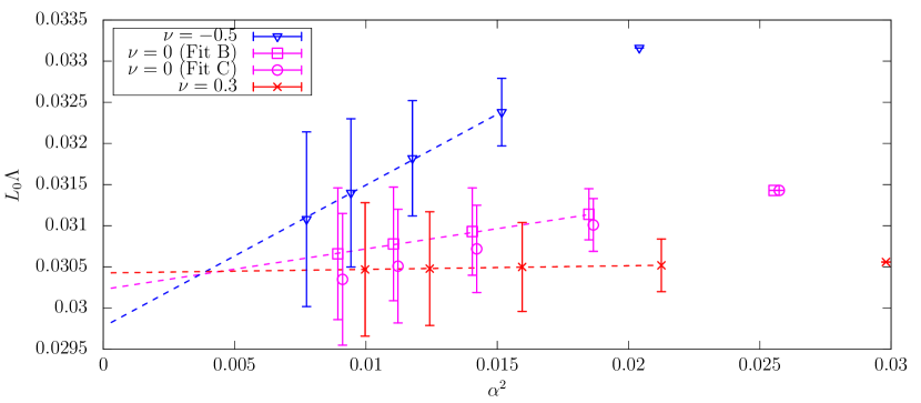
Figure 2: Adaptation of Fig. 2 of Ref. [89], kindly provided by Alberto Ramos. The figure shows the extraction of the QCD $\Lambda$ parameter, in units of $L_{0}\simeq 4.22\,\text{GeV}$, in the Schrödinger Functional scheme. Different lattice sizes (or correspondingly scales $\mu_{\text{PT}}$ in the step scaling approach) each lead to one $\alpha_{s}(\mu_{\text{PT}})$, the value of which is shown squared on the $x$ axis (labelled $\alpha^{2}$). For each $\alpha_{s}(\mu_{\text{PT}})$ result, the authors deduce a value for the QCD $\Lambda$ parameter ($y$ axis). The parameter $\nu$ in the underlying Schrödinger Functional approach can be thought of as a renormalisation scheme choice ($\Lambda$ is always converted back to a unique scheme). The two $\nu=0$ sets of results (labelled Fit B, C) correspond to different correction schemes for lattice discretisation artefacts.

A demonstration of the perturbative robustness of the ALPHA determination is given in Fig. 2, which shows the extraction of the QCD scale $\Lambda$ (defined in terms of $\alpha_{s}(\mu)$ in Eqs. (1,2) of Ref. [89]), based on a number of differently sized lattices, covering a factor of 16 in scales. For each lattice size, they determine a value of $\alpha_{s}$ at a scale $\mu_{\text{PT}}$ associated with the lattice size. Then using purely perturbative running they can convert it to a value for $\Lambda$. This is done for a variety of schemes, corresponding to the choices of $\nu$ in the figure (the $\Lambda$ value shown is defined in a scheme invariant way). With a $\beta$-function known to all orders and in the absence of power corrections, the extracted $\Lambda$ would be independent of $\mu_{\text{PT}}$ or correspondingly of the $\alpha_{s}^{2}(\mu_{\text{PT}})$ value shown on the $x$ axis. In practice, missing higher order terms for the $\beta$ function in the Schrödinger Functional scheme should correspond to a residual offset for the extracted $\Lambda$ value that scales as $\alpha_{s}^{2}(\mu_{\text{PT}}^{2})$, with a $\nu$-dependent coefficient. This is observed in the lattice data over the last three iterations of step scaling, insofar as the four leftmost points (covering a factor of $8$ in $\mu_{\text{PT}}$) are consistent with a linear dependence of the extracted $\Lambda$ parameter on $\alpha_{s}^{2}$. An extrapolation of $\Lambda$ to zero coupling is always consistent with the result at the lowest available value of $\alpha_{s}$, within its statistical errors. Furthermore, at that lowest value of $\alpha_{s}$, the different schemes are all in agreement. This is a powerful cross-check of the stability of the perturbative side of the extraction over a broad range of scales. The final uncertainty of $2.6\%$ on $L_{0}\Lambda$ that is quoted by the authors corresponds to about $0.54\%$ uncertainty on $\alpha_{s}(m_{Z})$. The conversion of these results to an $\overline{\text{MS}}$ $\Lambda$ (or coupling) in physical units, in particular the determination of $L_{0}$ in GeV, corresponds to the work of Refs. [91, 86].

One issue raised by the ALPHA collaboration is that their results (as most others) are for $2+1$ flavours, and so require perturbative matching at the charm mass in order to be interpreted as a 5-flavour coupling at $m_{Z}$. However, the 2015 HPQCD result with $2+1+1$ flavours [80] is very close to the earlier result with $2+1$ flavours and a perturbative charm threshold [7]. This suggests that non-perturbative charm-threshold effects are small. A further potential concern is that QED and isospin breaking effects are not accounted for in the lattice simulations of the low-energy hadronic quantities, however these are believed to be subdominant compared to the current uncertainties. Nevertheless, such points may need to be addressed in future higher-accuracy determinations of the strong coupling.

8 Concluding remarks

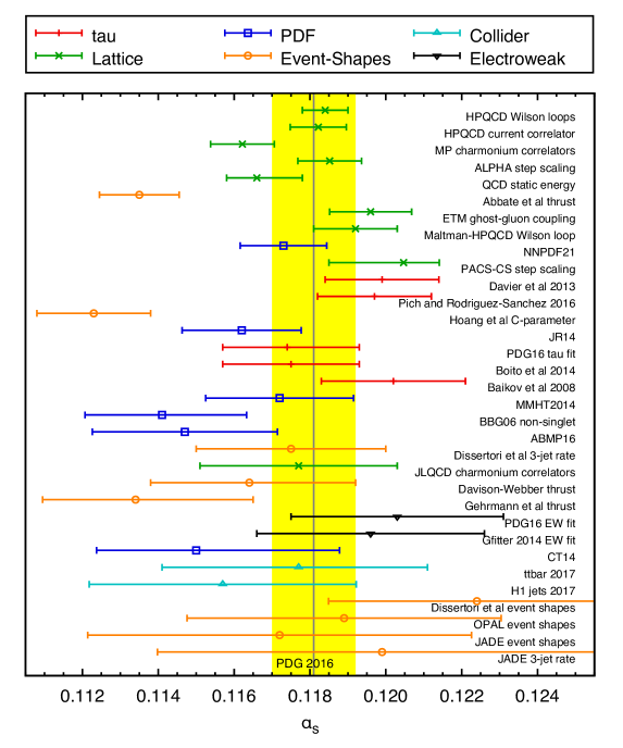
Figure 3: The $\alpha_{s}$ determinations discussed in this review, in order of increasing quoted uncertainty.

The many different (NNLO and better) determinations are summarised in Fig. 3. A wide range of methods can deliver results for $\alpha_{s}$ with an accuracy of a few percent. However such an accuracy is not sufficient if one is to fully exploit the results that are coming and still to come from the LHC. The question then for the field is which, if any, of the percent-level determinations to trust given that some of them are mutually incompatible. A few years ago, Guido’s answer to that question was, essentially, none!

The key issues that recur are the estimate of uncertainties from missing higher orders and the problem of non-perturbative corrections. Many of the determinations based on $\tau$ decays, event shapes, PDF fits and lattice methods are either directly determining $\alpha_{s}$ at a scale in the range of $1{-}3\,\text{GeV}$ or are in some other way sensitive to the physics occurring on those scales. Most of them give detailed reasoning as to why they believe they are able to control the problems that might arise from proximity to the non-perturbative region and the poor convergence of the series when $\alpha_{s}$ is not so small. However the accessible range of scales over which one can rigorously test these statements tends to be limited, leaving the door open to sometimes heated debate about the degree of control over systematic uncertainties.

In this respect the recent ALPHA lattice result is potentially a breakthrough. Together with EW precision fits, it is the only approach where the connection with perturbation theory is made at a genuinely high scale, with almost no assumptions needed about low-scale physics. Its precision of $0.7\%$ is almost three times better than the result from EW fits, thanks in part to the fact that it is not limited by LEP statistics. Furthermore the method can provide an extraction over a wide range of momentum scales and the pattern of results obtained in that way gives strong support to the authors’ arguments that the perturbative extraction is robust.

What would be needed to consolidate the ALPHA advance? Any determination of $\alpha_{s}$ that reaches percent-level accuracy tends to be a complicated endeavour, with aspects that can be adequately judged only by experts in that sub-field. That goes against the criterion of transparency called for by Guido. In such situations, sometimes the best way of judging a result is to attempt to reproduce it, ideally making complementary choices where relevant. A second, independent, up-to-date lattice step-scaling determination would thus be important to help establish this approach as the reference method for $\alpha_{s}$ determinations.

In the meantime, what global average should one use? For the 2017 PDG update we decided to maintain the 2016 average, $\alpha_{s}(m_{Z})=0.1181\pm 0.0011$ in order to allow more time to collect community input on the latest $\alpha_{s}$ determinations. This world average remains consistent with, if somewhat more conservative than, a simple weighted average of the two determinations that appear today to be the cleanest, namely the ALPHA and EW determinations, which gives $\alpha_{s}(m_{Z})=0.1186\pm 0.0008$.

Acknowledgements

Aside from those with Guido, I have benefited from discussions on $\alpha_{s}$ with many colleagues and friends over the years. In particular I would like to thank Siggi Bethke and Günther Dissertori for the past decade of collaboration on the PDG QCD review chapter, including discussions about all aspects of $\alpha_{s}$ determinations (and together with Thomas Klijnsma also our work on $\alpha_{s}$ from top-quark cross sections), as well as Jens Erler for regular discussions about aspects that overlap with the Electroweak review; Martin Lüscher, Luigi del Debbio and Agostino Patella, for numerous discussions about lattice approaches and Alberto Ramos for extensive exchanges on the ALPHA determination and for supplying Fig. 2; Martin Beneke and Toni Pich for their insights on $\tau$ determinations (if my conclusions differ from theirs it may simply be because I still have more to learn), as well as Andreas Höcker and Zhiqing Zhang for clarifications; Johannes Blümlein, Stefano Forte, Sven Moch, Juan Rojo and Robert Thorne for discussions about PDF fits; Andrea Banfi, Stefan Kluth, Gionata Luisoni, Pier Monni and Giulia Zanderighi for their insights about $e^{+}e^{-}$ jet rates and event shapes and their input for Fig. 1 as well as Günther Dissertori for permission to reproduce the top-right panel of Fig. 1; and, finally, Zoltán Trócsányi for discussions concerning the interplay of the strong coupling and vacuum stability. I would also like to thank Siggi Bethke, Michelangelo Mangano, Pier Monni, Alberto Ramos and Giulia Zanderighi for helpful comments on the manuscript.

References

- [1] S. Bethke et al., Workshop on Precision Measurements of , arXiv:1110.0016.
- [2] A. Pich, Review of determinations, arXiv:1303.2262. [PoSConfinementX,022(2012)].
- [3] S. Moch et al., High precision fundamental constants at the TeV scale, arXiv:1405.4781.
- [4] D. d’Enterria, ed., Proceedings, High-Precision Measurements from LHC to FCC-ee, (Geneva), CERN, CERN, 2015.
- [5] Particle Data Group Collaboration, C. Patrignani et al., Review of Particle Physics, Chin. Phys. C40 (2016), no. 10 100001.
- [6] G. Altarelli, The QCD Running Coupling and its Measurement, PoS Corfu2012 (2013) 002, [arXiv:1303.6065].
- [7] C. McNeile, C. T. H. Davies, E. Follana, K. Hornbostel, and G. P. Lepage, High-Precision c and b Masses, and QCD Coupling from Current-Current Correlators in Lattice and Continuum QCD, Phys. Rev. D82 (2010) 034512, [arXiv:1004.4285].
- [8] R. Abbate, M. Fickinger, A. H. Hoang, V. Mateu, and I. W. Stewart, Thrust at N3LL with Power Corrections and a Precision Global Fit for , Phys. Rev. D83 (2011) 074021, [arXiv:1006.3080].
- [9] S. Dulat, T.-J. Hou, J. Gao, M. Guzzi, J. Huston, P. Nadolsky, J. Pumplin, C. Schmidt, D. Stump, and C. P. Yuan, New parton distribution functions from a global analysis of quantum chromodynamics, Phys. Rev. D93 (2016), no. 3 033006, [arXiv:1506.0744].
- [10] M. Bonvini, S. Marzani, C. Muselli, and L. Rottoli, On the Higgs cross section at N3LO+N3LL and its uncertainty, JHEP 08 (2016) 105, [arXiv:1603.0800].
- [11] C. Anastasiou, C. Duhr, F. Dulat, E. Furlan, T. Gehrmann, F. Herzog, A. Lazopoulos, and B. Mistlberger, High precision determination of the gluon fusion Higgs boson cross-section at the LHC, JHEP 05 (2016) 058, [arXiv:1602.0069].
- [12] M. Czakon and A. Mitov, Top++: A Program for the Calculation of the Top-Pair Cross-Section at Hadron Colliders, Comput. Phys. Commun. 185 (2014) 2930, [arXiv:1112.5675].
- [13] S. Alekhin, J. Blümlein, S. Moch, and R. Placakyte, Parton distribution functions, , and heavy-quark masses for LHC Run II, Phys. Rev. D96 (2017), no. 1 014011, [arXiv:1701.0583].
- [14] LHC Higgs Cross Section Working Group Collaboration, D. de Florian et al., Handbook of LHC Higgs Cross Sections: 4. Deciphering the Nature of the Higgs Sector, arXiv:1610.0792.
- [15] ATLAS Collaboration, G. Aad et al., Measurement of the production cross-section using events with b-tagged jets in pp collisions at = 7 and 8 with the ATLAS detector, Eur. Phys. J. C74 (2014), no. 10 3109, [arXiv:1406.5375]. [Addendum: Eur. Phys. J.C76,no.11,642(2016)].
- [16] CMS Collaboration, V. Khachatryan et al., Measurement of the t-tbar production cross section in the e-mu channel in proton-proton collisions at sqrt(s) = 7 and 8 TeV, JHEP 08 (2016) 029, [arXiv:1603.0230].
- [17] J. R. Espinosa, G. F. Giudice, E. Morgante, A. Riotto, L. Senatore, A. Strumia, and N. Tetradis, The cosmological Higgstory of the vacuum instability, JHEP 09 (2015) 174, [arXiv:1505.0482].
- [18] S. Catani, Y. L. Dokshitzer, M. Olsson, G. Turnock, and B. R. Webber, New clustering algorithm for multi-jet cross-sections in annihilation, Phys. Lett. B269 (1991) 432–438.
- [19] Y. L. Dokshitzer, G. D. Leder, S. Moretti, and B. R. Webber, Better jet clustering algorithms, JHEP 08 (1997) 001, [hep-ph/9707323].
- [20] ALEPH Collaboration, A. Heister et al., Studies of QCD at centre-of-mass energies between 91-GeV and 209-GeV, Eur. Phys. J. C35 (2004) 457–486.
- [21] S. Weinzierl, Jet algorithms in electron-positron annihilation: Perturbative higher order predictions, Eur. Phys. J. C71 (2011) 1565, [arXiv:1011.6247]. [Erratum: Eur. Phys. J.C71,1717(2011)].
- [22] A. Gehrmann-De Ridder, T. Gehrmann, E. W. N. Glover, and G. Heinrich, Jet rates in electron-positron annihilation at in QCD, Phys. Rev. Lett. 100 (2008) 172001, [arXiv:0802.0813].
- [23] V. Del Duca, C. Duhr, A. Kardos, G. Somogyi, and Z. Trócsányi, Three-Jet Production in Electron-Positron Collisions at Next-to-Next-to-Leading Order Accuracy, Phys. Rev. Lett. 117 (2016), no. 15 152004, [arXiv:1603.0892].
- [24] T. Sjostrand, S. Mrenna, and P. Z. Skands, PYTHIA 6.4 Physics and Manual, JHEP 05 (2006) 026, [hep-ph/0603175].
- [25] G. Dissertori, A. Gehrmann-De Ridder, T. Gehrmann, E. W. N. Glover, G. Heinrich, and H. Stenzel, Precise determination of the strong coupling constant at NNLO in QCD from the three-jet rate in electron–positron annihilation at LEP, Phys. Rev. Lett. 104 (2010) 072002, [arXiv:0910.4283].
- [26] T. Sjöstrand, S. Ask, J. R. Christiansen, R. Corke, N. Desai, P. Ilten, S. Mrenna, S. Prestel, C. O. Rasmussen, and P. Z. Skands, An Introduction to PYTHIA 8.2, Comput. Phys. Commun. 191 (2015) 159–177, [arXiv:1410.3012].
- [27] P. Skands, S. Carrazza, and J. Rojo, Tuning PYTHIA 8.1: the Monash 2013 Tune, Eur. Phys. J. C74 (2014), no. 8 3024, [arXiv:1404.5630].
- [28] OPAL Collaboration, G. Abbiendi et al., Determination of alpha(s) using jet rates at LEP with the OPAL detector, Eur. Phys. J. C45 (2006) 547–568, [hep-ex/0507047].
- [29] JADE Collaboration, J. Schieck, S. Bethke, S. Kluth, C. Pahl, and Z. Trocsanyi, Measurement of the strong coupling from the three-jet rate in -annihilation using JADE data, Eur. Phys. J. C73 (2013), no. 3 2332, [arXiv:1205.3714].
- [30] G. Dissertori, A. Gehrmann-De Ridder, T. Gehrmann, E. W. N. Glover, G. Heinrich, G. Luisoni, and H. Stenzel, Determination of the strong coupling constant using matched NNLO+NLLA predictions for hadronic event shapes in annihilations, JHEP 08 (2009) 036, [arXiv:0906.3436].
- [31] JADE Collaboration, S. Bethke, S. Kluth, C. Pahl, and J. Schieck, Determination of the Strong Coupling alpha(s) from hadronic Event Shapes with and resummed QCD predictions using JADE Data, Eur. Phys. J. C64 (2009) 351–360, [arXiv:0810.1389].
- [32] OPAL Collaboration, G. Abbiendi et al., Determination of using OPAL hadronic event shapes at - 209 GeV and resummed NNLO calculations, Eur. Phys. J. C71 (2011) 1733, [arXiv:1101.1470].
- [33] R. A. Davison and B. R. Webber, Non-Perturbative Contribution to the Thrust Distribution in Annihilation, Eur. Phys. J. C59 (2009) 13–25, [arXiv:0809.3326].
- [34] T. Gehrmann, G. Luisoni, and P. F. Monni, Power corrections in the dispersive model for a determination of the strong coupling constant from the thrust distribution, Eur. Phys. J. C73 (2013), no. 1 2265, [arXiv:1210.6945].
- [35] A. H. Hoang, D. W. Kolodrubetz, V. Mateu, and I. W. Stewart, Precise determination of from the -parameter distribution, Phys. Rev. D91 (2015), no. 9 094018, [arXiv:1501.0411].
- [36] S. Brandt, C. Peyrou, R. Sosnowski, and A. Wroblewski, The Principal axis of jets. An Attempt to analyze high-energy collisions as two-body processes, Phys. Lett. 12 (1964) 57–61.
- [37] E. Farhi, A QCD Test for Jets, Phys. Rev. Lett. 39 (1977) 1587–1588.
- [38] R. K. Ellis, D. A. Ross, and A. E. Terrano, The Perturbative Calculation of Jet Structure in e+ e- Annihilation, Nucl. Phys. B178 (1981) 421–456.
- [39] S. Catani, G. Turnock, and B. R. Webber, Jet broadening measures in annihilation, Phys. Lett. B295 (1992) 269–276.
- [40] M. Beneke, Renormalons, Phys. Rept. 317 (1999) 1–142, [hep-ph/9807443].
- [41] M. Dasgupta and G. P. Salam, Event shapes in e+ e- annihilation and deep inelastic scattering, J. Phys. G30 (2004) R143, [hep-ph/0312283].
- [42] P. A. Baikov, K. G. Chetyrkin, and J. H. Kuhn, Order QCD Corrections to Z and tau Decays, Phys. Rev. Lett. 101 (2008) 012002, [arXiv:0801.1821].
- [43] P. A. Baikov, K. G. Chetyrkin, J. H. Kuhn, and J. Rittinger, Adler Function, Sum Rules and Crewther Relation of Order : the Singlet Case, Phys. Lett. B714 (2012) 62–65, [arXiv:1206.1288].
- [44] SLD Electroweak Group, DELPHI, ALEPH, SLD, SLD Heavy Flavour Group, OPAL, LEP Electroweak Working Group, L3 Collaboration, S. Schael et al., Precision electroweak measurements on the resonance, Phys. Rept. 427 (2006) 257–454, [hep-ex/0509008].
- [45] Gfitter Group Collaboration, M. Baak, J. Cúth, J. Haller, A. Hoecker, R. Kogler, K. Mönig, M. Schott, and J. Stelzer, The global electroweak fit at NNLO and prospects for the LHC and ILC, Eur. Phys. J. C74 (2014) 3046, [arXiv:1407.3792].
- [46] M. Davier, A. Höcker, B. Malaescu, C.-Z. Yuan, and Z. Zhang, Update of the ALEPH non-strange spectral functions from hadronic decays, Eur. Phys. J. C74 (2014), no. 3 2803, [arXiv:1312.1501].
- [47] ALEPH Collaboration, S. Schael et al., Branching ratios and spectral functions of tau decays: Final ALEPH measurements and physics implications, Phys. Rept. 421 (2005) 191–284, [hep-ex/0506072].
- [48] OPAL Collaboration, K. Ackerstaff et al., Measurement of the strong coupling constant alpha(s) and the vector and axial vector spectral functions in hadronic tau decays, Eur. Phys. J. C7 (1999) 571–593, [hep-ex/9808019].
- [49] G. Abbas, B. Ananthanarayan, I. Caprini, and J. Fischer, Perturbative expansion of the QCD Adler function improved by renormalization-group summation and analytic continuation in the Borel plane, Phys. Rev. D87 (2013), no. 1 014008, [arXiv:1211.4316].
- [50] D. Boito, M. Golterman, K. Maltman, and S. Peris, Strong coupling from hadronic decays: A critical appraisal, Phys. Rev. D95 (2017), no. 3 034024, [arXiv:1611.0345].
- [51] A. Pich and A. Rodríguez-Sánchez, Determination of the QCD coupling from ALEPH decay data, Phys. Rev. D94 (2016), no. 3 034027, [arXiv:1605.0683].
- [52] P. A. Baikov, K. G. Chetyrkin, and J. H. Kühn, Five-Loop Running of the QCD coupling constant, Phys. Rev. Lett. 118 (2017), no. 8 082002, [arXiv:1606.0865].
- [53] F. Herzog, B. Ruijl, T. Ueda, J. A. M. Vermaseren, and A. Vogt, The five-loop beta function of Yang-Mills theory with fermions, JHEP 02 (2017) 090, [arXiv:1701.0140].
- [54] K. G. Chetyrkin, J. H. Kuhn, and C. Sturm, QCD decoupling at four loops, Nucl. Phys. B744 (2006) 121–135, [hep-ph/0512060].
- [55] D. Boito, M. Golterman, K. Maltman, J. Osborne, and S. Peris, Strong coupling from the revised ALEPH data for hadronic decays, Phys. Rev. D91 (2015), no. 3 034003, [arXiv:1410.3528].
- [56] V. N. Gribov and L. N. Lipatov, Deep inelastic e p scattering in perturbation theory, Sov. J. Nucl. Phys. 15 (1972) 438–450. [Yad. Fiz.15,781(1972)].
- [57] G. Altarelli and G. Parisi, Asymptotic Freedom in Parton Language, Nucl. Phys. B126 (1977) 298–318.
- [58] Y. L. Dokshitzer, Calculation of the Structure Functions for Deep Inelastic Scattering and e+ e- Annihilation by Perturbation Theory in Quantum Chromodynamics., Sov. Phys. JETP 46 (1977) 641–653. [Zh. Eksp. Teor. Fiz.73,1216(1977)].
- [59] S. Alekhin, J. Blumlein, and S. Moch, Parton Distribution Functions and Benchmark Cross Sections at NNLO, Phys. Rev. D86 (2012) 054009, [arXiv:1202.2281].
- [60] J. Blumlein, H. Bottcher, and A. Guffanti, Non-singlet QCD analysis of deep inelastic world data at , Nucl. Phys. B774 (2007) 182–207, [hep-ph/0607200].
- [61] R. D. Ball, V. Bertone, L. Del Debbio, S. Forte, A. Guffanti, J. I. Latorre, S. Lionetti, J. Rojo, and M. Ubiali, Precision NNLO determination of using an unbiased global parton set, Phys. Lett. B707 (2012) 66–71, [arXiv:1110.2483].
- [62] P. Jimenez-Delgado and E. Reya, Delineating parton distributions and the strong coupling, Phys. Rev. D89 (2014), no. 7 074049, [arXiv:1403.1852].
- [63] L. A. Harland-Lang, A. D. Martin, P. Motylinski, and R. S. Thorne, Uncertainties on in the MMHT2014 global PDF analysis and implications for SM predictions, Eur. Phys. J. C75 (2015), no. 9 435, [arXiv:1506.0568].
- [64] S. Moch, B. Ruijl, T. Ueda, J. A. M. Vermaseren, and A. Vogt, Four-Loop Non-Singlet Splitting Functions in the Planar Limit and Beyond, JHEP 10 (2017) 041, [arXiv:1707.0831].
- [65] S. Alekhin, J. Blumlein, and S. Moch, The ABM parton distributions tuned to LHC data, Phys. Rev. D89 (2014), no. 5 054028, [arXiv:1310.3059].
- [66] R. S. Thorne, The effect on PDFs and due to changes in flavour scheme and higher twist contributions, Eur. Phys. J. C74 (2014), no. 7 2958, [arXiv:1402.3536].
- [67] J. Butterworth et al., PDF4LHC recommendations for LHC Run II, J. Phys. G43 (2016) 023001, [arXiv:1510.0386].
- [68] J. Currie, E. W. N. Glover, and J. Pires, Next-to-Next-to Leading Order QCD Predictions for Single Jet Inclusive Production at the LHC, Phys. Rev. Lett. 118 (2017), no. 7 072002, [arXiv:1611.0146].
- [69] L. A. Harland-Lang, A. D. Martin, and R. S. Thorne, The Impact of LHC Jet Data on the MMHT PDF Fit at NNLO, arXiv:1711.0575.
- [70] R. Boughezal, A. Guffanti, F. Petriello, and M. Ubiali, The impact of the LHC Z-boson transverse momentum data on PDF determinations, JHEP 07 (2017) 130, [arXiv:1705.0034].
- [71] ATLAS Collaboration, G. Aad et al., Measurement of the transverse momentum and distributions of Drell–Yan lepton pairs in proton–proton collisions at TeV with the ATLAS detector, Eur. Phys. J. C76 (2016), no. 5 291, [arXiv:1512.0219].
- [72] R. D. Ball, V. Bertone, M. Bonvini, S. Marzani, J. Rojo, and L. Rottoli, Parton distributions with small-x resummation: evidence for BFKL dynamics in HERA data, arXiv:1710.0593.
- [73] S. Dittmaier, Standard Model Theory, in 2017 European Physical Society Conference on High Energy Physics (EPS-HEP 2017) Venice, Italy, July 5-12, 2017, 2017. arXiv:1709.0856.
- [74] CMS Collaboration, S. Chatrchyan et al., Determination of the top-quark pole mass and strong coupling constant from the production cross section in pp collisions at = 7 TeV, Phys. Lett. B728 (2014) 496–517, [arXiv:1307.1907]. [Erratum: Phys. Lett.B738,526(2014)].
- [75] T. Klijnsma, S. Bethke, G. Dissertori, and G. P. Salam, Determination of the strong coupling constant from measurements of the total cross section for top-antitop quark production, Eur. Phys. J. C77 (2017), no. 11 778, [arXiv:1708.0749].
- [76] M. Czakon, P. Fiedler, and A. Mitov, Total Top-Quark Pair-Production Cross Section at Hadron Colliders Through , Phys. Rev. Lett. 110 (2013) 252004, [arXiv:1303.6254].
- [77] H1 Collaboration, V. Andreev et al., Determination of the strong coupling constant in next-to-next-to-leading order QCD using H1 jet cross section measurements, Eur. Phys. J. C77 (2017), no. 11 791, [arXiv:1709.0725].
- [78] J. Currie, T. Gehrmann, and J. Niehues, Precise QCD predictions for the production of dijet final states in deep inelastic scattering, Phys. Rev. Lett. 117 (2016), no. 4 042001, [arXiv:1606.0399].
- [79] K. Maltman, D. Leinweber, P. Moran, and A. Sternbeck, The Realistic Lattice Determination of Revisited, Phys. Rev. D78 (2008) 114504, [arXiv:0807.2020].
- [80] B. Chakraborty, C. T. H. Davies, B. Galloway, P. Knecht, J. Koponen, G. C. Donald, R. J. Dowdall, G. P. Lepage, and C. McNeile, High-precision quark masses and QCD coupling from lattice QCD, Phys. Rev. D91 (2015), no. 5 054508, [arXiv:1408.4169].
- [81] K. Nakayama, B. Fahy, and S. Hashimoto, Short-distance charmonium correlator on the lattice with Möbius domain-wall fermion and a determination of charm quark mass, Phys. Rev. D94 (2016), no. 5 054507, [arXiv:1606.0100].
- [82] Y. Maezawa and P. Petreczky, Quark masses and strong coupling constant in 2+1 flavor QCD, Phys. Rev. D94 (2016), no. 3 034507, [arXiv:1606.0879].
- [83] ETM Collaboration, B. Blossier, P. Boucaud, M. Brinet, F. De Soto, V. Morenas, O. Pene, K. Petrov, and J. Rodriguez-Quintero, High statistics determination of the strong coupling constant in Taylor scheme and its OPE Wilson coefficient from lattice QCD with a dynamical charm, Phys. Rev. D89 (2014), no. 1 014507, [arXiv:1310.3763].
- [84] A. Bazavov, N. Brambilla, X. Garcia i Tormo, P. Petreczky, J. Soto, and A. Vairo, Determination of from the QCD static energy: An update, Phys. Rev. D90 (2014), no. 7 074038, [arXiv:1407.8437].
- [85] PACS-CS Collaboration, S. Aoki et al., Precise determination of the strong coupling constant in N(f) = 2+1 lattice QCD with the Schrodinger functional scheme, JHEP 10 (2009) 053, [arXiv:0906.3906].
- [86] ALPHA Collaboration, M. Bruno, M. Dalla Brida, P. Fritzsch, T. Korzec, A. Ramos, S. Schaefer, H. Simma, S. Sint, and R. Sommer, QCD Coupling from a Nonperturbative Determination of the Three-Flavor Parameter, Phys. Rev. Lett. 119 (2017), no. 10 102001, [arXiv:1706.0382].
- [87] HPQCD Collaboration, C. T. H. Davies, K. Hornbostel, I. D. Kendall, G. P. Lepage, C. McNeile, J. Shigemitsu, and H. Trottier, Update: Accurate Determinations of from Realistic Lattice QCD, Phys. Rev. D78 (2008) 114507, [arXiv:0807.1687].
- [88] S. Aoki et al., Review of lattice results concerning low-energy particle physics, Eur. Phys. J. C74 (2014) 2890, [arXiv:1310.8555].
- [89] ALPHA Collaboration, M. Dalla Brida, P. Fritzsch, T. Korzec, A. Ramos, S. Sint, and R. Sommer, Determination of the QCD -parameter and the accuracy of perturbation theory at high energies, Phys. Rev. Lett. 117 (2016), no. 18 182001, [arXiv:1604.0619].
- [90] M. Lüscher, P. Weisz, and U. Wolff, A Numerical method to compute the running coupling in asymptotically free theories, Nucl. Phys. B359 (1991) 221–243.
- [91] ALPHA Collaboration, M. Dalla Brida, P. Fritzsch, T. Korzec, A. Ramos, S. Sint, and R. Sommer, Slow running of the Gradient Flow coupling from 200 MeV to 4 GeV in QCD, Phys. Rev. D95 (2017), no. 1 014507, [arXiv:1607.0642].