Non-Abelian Charge Transport in Three-Flavor Gauge Semimetal Model with Braiding Majoranas

Abstract

Known Majorana fermions models are considered as promising ones for the purposes of quantum computing robust to decoherence. One of the most expecting but unachieved goals is an effective control for braiding of Majoranas. Another one is to describe ${\mathbb{Z}}_{2}$ topological semimetals, APRES spectra of which testify on eight-fold degenerate chiral fermions with $SU(2)$ holonomy of wave functions, whereas the last can not be reproduced within existing models. Quasi-relativistic theory of non-abelian quantum charge transport in topological semimetals is developed for a model with a number of flavors equal three. Majorana-like quasi-particle excitations in the model are described with accounting of dynamic mass term arising due to relativistic exchange interactions. Such exotic features of $\mathbb{Z}_{2}$ semimetals as splitting zero-conductance peaks, longitudinal magnetoresistance, minimal direct current conductivity, negative differential conductivity have been calculated in perfect agreement with experimental data. We propose a new scheme of braiding for three flavor Majorana-like fermions with new non-trivial braiding operator. We demonstrate that in this model, the presence of chiral Majorana-like bound states is controlled as emergence of three pairs of resonance-antiresonance in frequency dependence of dielectric permeability.

I Introduction

Topological semimetals (SMs) are graphene-like materials with touching and non-overlapping valence and conduction bands. SMs can exhibit unique magneto-electrical properties, including an angle-dependent magnetoresistance Luo-McDonald-Rosa-SciRep2016 ; Q-Li-ChiralNat-Phys2016 ; Du-Wang-Chen-Sci.-China-Phys2016 ; Yan-Zhang-Liu-Liu-Zhang-Xiu-Zhou ; H-ZhLuSh-QShen2017 , ultrahigh electroconductivity Cooper2012 ; Bolotin-Sikes-SolidStateCom2008 ; Wang-Weng-Wu-PhysRev2013 ; Liang-Gibson-Ali-NatMat2015 ; Son-Spivak-PhysRev2013 , as well as ultrahigh radiation resistance Huang-GrapheneDamage-SciRep2016 . Experiments the charge transport in Dirac materials (graphene, two-dimensional (2D) semimetals and three-dimensional (3D) topological insulators (TI) or, more precisely, chiral edge gapless 3D-TI-modes) have revealed a chiral anomaly of their transport properties and simultaneously signatures of zero-energy Majorana modes Huang-Zhao-Long-PhysRevX2015 . Berry curvature for the monolayer graphene model diverges in touching points between valence and conduction bands (Dirac points of the Brillouin zone, also called valleys) Xiao-Chang-Niu2010Rev-Mod-Phys . The existence of topological currents in graphene superlattices has been proposed in Science346-2014Gorbachev . In graphene, signatures of Majorana excitation have been experimentally observed in PhysRevX5-2015San-Jose . Majorana zero-energy modes are new type of quasiparticles, which have been theoretically predicted in high-$T_{c}$ topological p-wave superconductors (Majorana zero-energy modes and gapped Fermi arcs in angle-resolved photoemission spectra (ARPES) RepProgPhys-71-2008Lee ; SciTechnolAdvMater15-2014Wu ) Physics-Uspekhi44-2001Kitaev ; JPhysB40-2007Semenoff ; ElJTherPhys3-2006Semenoff ; PhysicsEMajorana-2014Wilczek and have been experimentally discovered in a ferromagnetic atomic chain (one-dimensional quantum wire) placed on the surface of a conventional s-superconductor Science346-2014Nadj-Perge . A Majorana fermion is its own antiparticle $\chi=\chi^{\dagger}$ E.Majorana1937 . A Dirac mass fermion $\psi$ can be represented as a particle formed from two Majorana fermions (MFs) $\chi_{1}$, $\chi_{2}$: $\psi=(\chi_{1}+i\chi_{2})/2$, $\psi^{*}=(\chi_{1}-i\chi_{2})/2$, and Majorana, accordingly, can be considered as a particle–hole pair from the Dirac fermions. Here ”^∗” denotes the complex conjugation.

The construction of quantum devices based on Dirac materials is a challenge because of the lack of understanding of deep connection of their unique electrical properties with the Majorana pattern (texture) of Dirac-fermions pairs in SM, and as a consequence, the deficit of simulation methods.

Let us assume that a Majorana fermion can be self-fissionable with subsequent self-fusion. Provided the presence of such a mechanism of existence of the Majorana particles, an external electromagnetic field would separate charged Majorana states in space and time, resulting in charge transport. Such representation of Majorana particle has been called a braiding representation in Nayak-Simon-RevModPhys2008 . Braiding operators on a set of Majoranas exist and form a unitary representation of the circular Artin braid group Kauffman-Lomonaco-Jr2016ArXiv . The materials with braiding Majorana excitations are known to be promising materials for quantum computing by quantum tunneling Physics-Uspekhi44-2001Kitaev ; JPhysB40-2007Semenoff ; JETPLetters103-2016Zyuzin ; arXiv1612-09276v1-2016 . Unfortunately, physical grounds of the 2D-braiding are unknown, in spite of the fact that braiding Majorana fermions by Ising spin 1D-chains have been proposed in Backens-Shnirman-Makhlin2017ArXiv .

Particles and holes in 2D and 3D Dirac semimetals (graphene Semenoff1984 ; Novoselov2005 ; Neto2009 ; Cooper2012 , Na₃Bi Science343-2014Liu ; Science347-2015Xu , Cd₃As₂ NatCommun5-2014Neupane ; PhyRevLett113-2014LBorisenko ; NatMater13-2014Jeon , perovskite SM Yan-Zhang-Liu-Liu-Zhang-Xiu-Zhou ) are massless. But Majorana equation of motion for ultrarelativistic massless fermions is not an oscillatory one E.Pessa2006JTheorPhys , and, accordingly, massless Majorana fermions can not represent a secondary quantized field. One can overcome this obstacle using Majorana-like equations derived in mySymmetry2016 for quasi-particle massless excitations in SM.

Degeneration of the Dirac bands is removed in the Weyl SM Lu-Shen2017Front-Phys ; Hubener_Sentef_Giovannini_Kemper_Rubio with the Dirac point, splitting into two massless Weyl nodes, and with gapless Fermi arcs in ARPES observations for TaAs family of such materials Science-349-2015 ; PhysRevX-5-2015 ; NatPhys-11-2015Lv ; NatPhys-11-2015Xu ; NatPhys11-2015Yang ; AnnualRevCondMattPhys2017Hasan ; Chin-Phys-Lett2015NbP . Hypothetically, one can assume that after pairing of Weyl nodes, nontrivial gapless surface states from the Weyl band structure are transformed into Majorana surface modes inside the pairing gap as Majorana and Fermi arcs in ARPES for a magnetic Weyl semimetal in superconducting state Li-Haldane2015arXiv ; Scientific-Reports6-2016ChangHasan ; BRoy2016arXiv .

Moreover, some topological SMs with/without spin-orbit coupling (SOC) or when spin-orbit interaction being neglected are nodal-line/ring semimetals PhysRevLett115-2015Kim ; PhysRevB92-2015ChenFang ; NatCommunic7-2016Bian . The 1D nodal-line states, which possess mirror reflection (inversion) coexisting with time reversal and an additional non-symmorphic symmetries (screw axis), are symmetry-protected so they are stable against perturbations, including SOC Science353-2016Bradlyn ; PhysRevB92-2015ChenFang ; PhysRevLett116-2016Wieder ; PhysRevX6-2016Muechler ; Yang-Yang-Derunova2017ArXiv . The nodal-line state enhances the surface Rashba splitting NatComunnic8-2017Hirayama . The 2D drumhead-like surface states inside the closed nodal ring are nested between conduction and valence bands Weng-Liang-Xu2015PhysRev ; Burkov-Hook2011PhysRev ; Hasan-Drumhead2016PhysRev ; Schnyder-Ca3P2PhyRev2016 ; Heikkila-Volovik2011JETP ; Marzari-Mostofi2012RevModPhys ; Xu-Yu-Fang-Dai-Weng2017PhysRev . The flat band surface states, density of which is very high, are similar to those in a high-temperature superconductor Kopnin-Heikkil2011PhysRev ; Heikkil-Kopnin2011JETP . A nodal-line no-magnetic semimetal PbTaSe₂ where the Pb-conducting orbitals (the particle-like 6p-Pb bands around $\overline{K}$, which inevitably cross the hole-like 5d-Ta bands with similar energy, leading to formation of the nodal rings) form the topological nodal-line states, is a candidate to a topological superconductor with nontrivial gapless surface states NatCommunic7-2016Bian ; PhysRevB93-2016Cheng-LongZhang . The nodal lines in PbTaSe₂ with strong SOC are protected by a reflection symmetry of the space group NatCommunic7-2016Bian . The massless chiral Majorana modes in PbTaSe₂ are placed on a 1D contour contrary to the Majorana zero-energy modes localized at 0D points.

Right- and left-hand particles always appear in pairs in virtue of the helicity conservation law and can not change their helicity as they are massless. Hence, there must be a mechanism that allows particles to exist only at one of the touching bands. Therefore, the graphene-like materials with chiral symmetry or 3D-TI-modes can be described using a mass term taking zero values at Dirac points, provided the chirality of the remaining ”single valley” particle is preserved. Similar problem of chiral anomaly in high energy physics has been treated in the following way. For ”single valley” massless Dirac fermions, a similar mass term could correspond to the so-called Wilson mass term which vanishes at momentum $\vec{k}=0$ and frequency $\omega=0$. But the Wilson mass term explicitly breaks the chiral symmetry Ginsparg-Wilson1982PhysRevD . Known receipt of its restoration Moran-Leinweber2011PhysLett ; Kaplan-Sun2012PhysRevLett ; Vafek-Vishwanath2013ArXiv is to find a lattice Dirac Hamiltonian with a sign alternating mass term on a space-like surface in such a way that the mass would be zero-valued on all lattice sites rather than in the origin only. The last leads to emergence of the zero-energy mode. A mass term (eigenvalues of the mass operator) entering into the equation of motion for the Majorana particle should be alternating one due to positive and negative values of the mass for Dirac particles and anti-particles respectively. Therefore, the use of Majorana representation is the way to the chiral theory of SMs. In a Dirac Hamiltonian describing 3D materials with band inversion H.Zhang2009NatPhys ; C.-X.Liu2010PhysRev a mass term is a sign alternating one as a Majorana mass term and similar to the Wilson term it gains zero value in the Dirac-like point. The band inversion is typical for 3D TIs, for example for Bi₂Se₃ Fu-Kane2007PhysRev where the inversion takes place in $\Gamma$-point of the Brillouin zone.

The discovery of Dirac materials with nodal line surrounding drumhead-like surface states has shown that the construction of a 2D Hamiltonian by adding a sign alternating mass term is limited to the cases when the entire nodal line can be placed on a zero mass surface.

SOC in the absence of inversion and time reversal symmetries breaks a nodal line into separate Weyl nodes as it has been calculated in Scientific-Reports6-2016ChangHasan ; Fang2016WengarXiv ; PhysRevB93-2016Hung-Liu-Vanderbit ; PhysRevB94-2016Narayan ; ChinesePhysB25-2016Weng-Dai . However SOC and odd-parity pairing can realize MFs in the nodal topological superconductor phase ScieAdv2-2016Kozil . Moreover, in the stoichiometric high-T_c superconductor (SC) YBa₂Cu₄O₈ under pressure, the quasiparticle mass decreases as the critical temperature T_c increases ScieAdv2-2016Putzke . Vortex cores in topological SCs host braiding MFs SciTechnolAdvMater15-2014Wu .

Thus, though Dirac materials are emerging topological phases with emergent Dirac Novoselov2005 , Weyl Nielsen-Ninomiya1983PhysLettB , and Majorana fermions Physics-Uspekhi44-2001Kitaev ; LiangFu-Kane2008PRL , Majorana representation should be a background for the description of their properties and charge transport. This explains the fact that the first-principles band-structure calculations, which are based on the usage of one-particle quasi-relativistic Dirac equation, demonstrate bands crossing but ”cannot serve as a proof of the Fermi arcs”  as it has been mentioned in NatureMaterials15-2016ShuangJiaS-YXu-MZHasan . There is a necessity in new theoretical approaches to design nodal-line structures and topological phases ”linked” with them FrontPhys12-2017YuFangDai .

Dichroism of s-polarized ARPES-spectra has been observed for TIs Bi₂Se₃, Bi₂Te₃ in Cao2013NatPhys ; Zhang-Liu-Zhang2013PRL ; Zhu-Layer-by-layer2013PRL and for NbP in Chin-Phys-Lett2015NbP . Dichroism puts forward the problem to find a Hamiltonian preserving the chiral symmetry of the Dirac cone bands, rather than a set of Dirac cone apexes (the Dirac points in the Brillouin zone). Hence, the search for the SM Hamiltonian should be based on new approaches such as the addition of an sign alternating mass term, which gets zero values on the surface of the Brillouin zone, rather than in distinct Dirac points.

Space of TI states is a space of even dimensionality $d$, $d=2$, in which an infinite number of pairs of oppositely twisted vortices with nontrivial topological charges emerges in accord with the Nielsen -Ninomiya ”no-go” –theorem on the existence of vortex lattices in only even dimensionality of the space Nielsen-Ninomiya1NuclPhys1981 ; Nielsen-Ninomiya2NuclPhys1981 ; MontvayMunster1997 . The proliferation of these vortices drives the Berezinskii -Kosterlitz -Thouless transition in a standard way JPhysC6-1973KosterlitzThouless . The only way to preserve the chirality of all the vortex ”single valley” nodes simultaneously with introducing the sign alternating mass term, is to use a singular (divergent) mass operator. The massless Weyl nodes in Weyl SMs were considered as topological defect structures (vortices) JPhysC5-1972KosterlitzThouless of the type of $U(1)$ gauge fields named as skyrmions, or a $SU(2)\ ($O(4)$)$ gauge fields named as merons (half skyrmions) in Supercond-Sci-Technol1988 , or $O(3)$ non-linear sigma models in NuclPhys336-1990Shankar . There is a good coincidence of experimental data with theoretical predictions on topological quantum phase transitions in 1D XY universality class, which includes different realizations of vortex-chain configurations in the continuum limit for free fermions JPhysC6-1973KosterlitzThouless ; PhysicsLettA93-1983Haldane ; PhysRevLett50-1983Haldane ; RevModPhys69-1997Sondhi ; PhysRevB81-2010Pollmann . Multiple vortices creation is observed in graphene and topological insulators in an electromagnetic field at lowering the symmetry of the structure Science340-2013Hunt ; SciAdv2-2016SanfengWu .

A resonating-valence-bond (RVB) picture Anderson1973 ; Fazekas-Anderson1974 ; Affleck-Marston1988 ; MySupercinductivity2010 and its quantum mechanical 1D-formulation MySupercinductivity2010 model a Fermi arc in ARPES spectrum as a break of the double conjugated chemical bond located on the left (right) side of a certain lattice site with the subsequent formation of the same bond between electrons of this site and electrons of the right(left) site to the considered one. The RVB picture has been formulated statistically in terms of skyrmions or merons Sachdev1992 ; Nagaosa-Lee1992 ; Wen-Lee1996 . In these field theories, defect staggered spin flows Hsu-Marston-Affleck1991 originated from RVB breaks are cores of vortices. But, skyrmions do not carry an electric charge, therefore, to overcome the obstacle, complex constructions with additional quasiparticles (holons) have been developed Kivelson-Rokhsar-Sethna1987 to describe the high $T_{c}$ conductivity. Moreover, the coupling of massless fermions to gauge fields in the $O(4)$ ($SU(2)$) non-linear sigma models is confining. Assuming violation of $SU(2)$ to $U(1)$ as a deconfinement one gets the so called triple quantum electrodynamics (QED₃ model) Vafek-Tesanovic-Franz2002 ; Lee-Herbut . To make a deconfined state stable, the number of matter fields should be large enough Hermele-Senthil-Fisher-Lee-Nagaosa-Wen . The zero-energy Majorana bound state (MBS) is associated with the non-abelian excitation. The vortex leads to the MBS, for example, in a superconductor $p_{x}+ip_{y}$ Read-Green2000PhysRev ; Ivanov2001PhysRev ; SternOppenMariani2004PhysRev ; StoneChung2006PhysRev .

Thus, to describe nodal-line Weyl semimetals a new theory is required, which would predict a phenomenon similar to deconfinement, and would be characterized by a sufficiently large number $N$ of gauge fields.

Another difficulty is that the Fermi arcs are not closed, because of that, the Fermi pockets are not formed. From the Luttinger theorem it follows that the area of the Fermi surface is the same as that of free fermions, i.e. it is determined by the total density of electrons in the unit cell Abrikosov-Gorkov-Dzyaloshinskii1965 . Violation of the Luttinger theorem in Landau–Fermi liquid theory leads to a non-conservation of the total electric charge. Therefore, if the Fermi pockets are not formed, then the violation of the Luttinger theorem becomes unavoidable obstacle in utilizing Dirac particle physics Oshikawa2000 ; Paramekanti-Vishwanath2004 to describe strongly correlated systems. The Majorana representation allows any fermionic system, either fermion number conserving or not, to be treated on equal footing Jaffe-Pedrocchi2015Annales-Henri-Poincare ; Bender-Mannheim2010 ; Wei-Congjun-Li-Zhang-Xiang2016 . The nodal lines restore the Fermi pockets and surround drumhead-like states PhysRevX6-2016Muechler ; PhysRevB93-2016Hung-Liu-Vanderbit ; the last gives hope for the construction of a field theory of Dirac materials provided one understood the origin and mechanisms of the decay of these lines.

Complex magnetic dynamics is developed in double perovskite compounds Ba₂YMoO₆, Ba${}_{2}Me$OsO₆($Me$ = Li, Na) despite of perfect cancelation of spin and angular momentum contributions at cubic symmetry Cussen-Lynham-Rogers2006 ; Aharen-Magnetic-properties2010 ; Vries-Mclaughlin-Bos2010 ; Carlo-Triplet2011 ; Steele-Low-moment-magnetism2011 . This testifies that SOC can effectively augment the Hubbard correlations effects in Mott- Hubbard physics Covalency-and-vibronic-couplings2016 ; Minimal-ingredients2016 .

So, quantum statistics of many-body systems with a particle-hole symmetry should be a non-abelian one, the absence of which is the main obstacle in investigation of Majorana-like states.

In the paper we develop a quantum non-abelian statistical approach to (pseudo)Majorana fermionic systems with calculus of quasi-relativistic currents and analyze emergent Majorana-like features of quantum charge transport in the Dirac materials.

We demonstrate that natural background to describe all types of Dirac materials is in accounting of relativistic exchange interactions, which destroy pseudo antiferromagnetic order in the Majorana basis. In Section 2 we construct a transformation which produces one-to-one map of quasiparticle states (hole (particle)) with the negative (positive) energy in one of two trigonal sublattices to states (particle (hole)) of the positive (negative) energy in other trigonal sublattice of the hexagonal lattice. Utilizing this transformation we find the equations of motion for a (pseudo)real braiding Majorana quasiparticle (electrically charged exciton) on a 2D hexagonal lattice. In Section 3 we develop a relativistic theory of the secondary-quantized field with a number of flavors $N=3$ on a hexagonal lattice within the quasi-relativistic Dirac–Hartree–Fock self-consistent field approximation we-Kazan ; we-arxiv2013 ; myNPCS2013 ; myNPCS17-2014 ; myarXiv1401-6880v1-2014 ; myJModPhys2014 ; myNATO2015 ; NPCS18-2015GrushevskayaKrylovGaisyonokSerow ; myNPCS18-2015 ; myTaylorFrancis2016 ; myIntJModPhys2016 . In the section we also demonstrate that the relativistic exchange leads to dynamically gapped Fermi arcs in topological semimetals. We use the $\vec{k}\cdot\vec{p}$ perturbation theory and maximally-localized Wannier functions, which provide accurate characterization of points of interest in the Brillouin zone (BZ) in terms of a relatively small number of parameters with the first-principles accuracy and linear-scaling computational costs. Opposite to known non-relativistic $\vec{k}\cdot\vec{p}$ approaches k-p_method2009Springer-Verlag ; LuttingerPhyRev1955 ; DresselhausKipKittel1955PhysRev ; Kormanyos2D2015 ; Yo-SLeeNardelliMarzari2005ArXiv ; Mostofi2008ComputPhysCommun ; Marzari-Mostofi2012RevModPhys ; Xu-Yu-Fang-Dai-Weng2017PhysRev95 , we propose a quasi-relativistic chiral band structure theory. Calculating Majorana bands in Section 3, we neglect the Majorana dynamical mass. However, the presence of heavy and light carriers is considered as a mass correction to complex conductivity in Section 4. In Section 5 splitting zero-conductance peaks, longitudinal magnetoresistance, minimal direct current (dc) conductivity, negative differential conductivity, appearance of Majorana resonance and anti-resonance pairs in frequency dependence of dielectric permeability and other phenomena of Majorana braiding in charge transport in topological SMs are predicted within a non-abelian quantum statistical approach developed in Section 4.

II Pseudo Majorana fermion model

Equation of motion for a Majorana bispinor $(\psi_{AB}^{\dagger},(\psi^{*}_{BA})^{\dagger})$ in a monoatomic hexagonal layer (monolayer), comprised of two trigonal sublattices $A,\ B$ reads myNPCS18-2015 ; mySymmetry2016 :

$$\left[\vec{\sigma}_{2D}^{BA}\cdot\vec{p}_{AB}-c^{-1}\widetilde{\Sigma_{AB}\Sigma_{BA}}\right]\left|\psi_{AB}\right\rangle=i{\partial\over\partial t}\left|\psi^{*}_{BA}\right\rangle,$$ (II.1)

$$\left[\vec{\sigma}_{2D}^{AB}\cdot\vec{p}\,^{*}_{BA}-c^{-1}\left(\widetilde{\Sigma_{BA}\Sigma_{AB}}\right)^{*}\right]\left|\psi^{*}_{BA}\right\rangle=-i{\partial\over\partial t}\left|\psi_{AB}\right\rangle.$$ (II.2)

Here, the sublattice wave functions $\left|\psi_{AB}\right\rangle$ and $\left|\psi^{*}_{BA}\right\rangle$ relate to each other as follows:

$$\left|\psi^{*}_{BA}\right\rangle\propto\left(\Sigma_{rel}^{x}\right)_{BA}\left|\psi_{AB}\right\rangle,$$ (II.3)

$$\left|\psi_{AB}\right\rangle\propto\left(\Sigma_{rel}^{x}\right)_{AB}\left|\psi^{*}_{BA}\right\rangle;$$ (II.4)

$\left(\Sigma_{rel}^{x}\right)_{AB}\equiv\Sigma_{AB},\ \left(\Sigma_{rel}^{x}\right)_{BA}\equiv\Sigma_{BA}$ are the relativistic exchange interaction operators for the trigonal sublattices $A,\ B$ of the hexagonal lattice; the dynamic mass operator terms $\widetilde{\Sigma_{BA(AB)}\Sigma_{AB(BA)}}$ are defined as

$$\widetilde{\Sigma_{BA(AB)}\Sigma_{AB(BA)}}=\left(i\Sigma_{rel}^{x}\right)_{BA(AB)}\left(i\Sigma_{rel}^{x}\right)_{AB(BA)};$$ (II.5)

a transformed 2D vector $\vec{\sigma}_{2D}^{AB}$ of the Pauli matrices and a transformed 2D momentum $\vec{p}_{BA(AB)}$ are introduced as

$$\vec{\sigma}_{2D}^{BA(AB)}=\left(\Sigma_{rel}^{x}\right)_{BA(AB)}\vec{\sigma}\,\left(\Sigma_{rel}^{x}\right)_{BA(AB)}^{-1},$$ (II.6)

$$\vec{p}_{BA(AB)}=\left(\Sigma_{rel}^{x}\right)_{BA(AB)}\vec{p}\,\left(\Sigma_{rel}^{x}\right)_{BA(AB)}^{-1};$$ (II.7)

$\vec{\sigma}$ is the 2D vector of the Pauli matrices: $\vec{\sigma}=\{\sigma_{1},\ \sigma_{2}\}$; $\vec{p}$ is the 2D momentum operator, $c$ is the speed of light. One can see, that when neglecting the operator (II.5), Eqs. (II.1), (II.2) are equations of motion for a Majorana-like massless particle.

The system of Eqs. (II.1), (II.2) can be approximated by a Dirac-like equation in the following way. Let us rewrite, for example, (II.1) for the steady state

$$\left[\vec{\sigma}_{2D}^{BA}\cdot\vec{p}_{AB}-c^{-1}\widetilde{\Sigma_{AB}\Sigma_{BA}}\right]\left|\psi_{AB}\right\rangle=E_{qu}\left|\psi^{*}_{BA}\right\rangle.$$ (II.8)

According to (II.6) and (II.7), the bispinor component $\left|\psi_{AB}\right\rangle$ can be obtained as $\left|\psi_{AB}\right\rangle=\Sigma_{AB}\left|\tilde{\psi}_{A}\right\rangle$. Due to (II.3) $\left|\tilde{\psi}_{A}\right\rangle$ also defines the component of the Majorana spinor $\left|\psi^{*}_{BA}\right\rangle$ as $\left|\psi^{*}_{BA}\right\rangle\propto\left(\Sigma_{rel}^{x}\right)_{BA}\left|\tilde{\psi}_{A}\right\rangle$. Hence

$$\Sigma_{BA(AB)}^{2}\propto\Sigma_{BA(AB)}.$$ (II.9)

Owing to the condition (II.9) and taking into account that in accord with (II.4) the operator $\Sigma_{AB}$ can be considered as a Fermi velocity operator $\hat{v}_{F}$ in (II.8), the following expansion holds up to normalization constant $\left<0\right|\hat{v}_{F}\left|0\right>$:

$$\left|\psi_{AB}\right\rangle\propto\Sigma_{AB}{\Sigma_{BA}\over\left<0\right|\hat{v}_{F}\left|0\right>}\left|\psi_{AB}\right\rangle={1\over\left<0\right|\hat{v}_{F}\left|0\right>}\left\{\Sigma_{BA}\left|\psi_{AB}\right\rangle+\left[\Sigma_{AB},\Sigma_{BA}\right]\left|\psi_{AB}\right\rangle\right\}\approx\left\{1+{\left(\Delta\Sigma+\left[\Sigma_{AB},\Sigma_{BA}\right]\right)\over\left<0\right|\hat{v}_{F}\left|0\right>}\right\}\left|\psi_{AB}\right\rangle$$

(II.10)

where $\left[\cdot,\cdot\right]$ denotes the commutator, $\Delta\Sigma=\Sigma_{BA}-\Sigma_{AB}$. Substituting (II.4, II.10) into the right-hand side of the equation (II.8), one gets the basic Dirac-like equation in the following form:

$$\left[\vec{\sigma}_{2D}^{BA}\cdot\vec{p}_{AB}-c^{-1}\widetilde{\Sigma_{AB}\Sigma_{BA}}\right]\left|\psi_{AB}\right\rangle=\tilde{E}\left\{1+\left(\Delta\Sigma+\left[\Sigma_{AB},\Sigma_{BA}\right]\right)/\left<0\right|\hat{v}_{F}\left|0\right>\right\}\left|\psi_{AB}\right\rangle$$ (II.11)

where $\tilde{E}=E/\left<0\right|\hat{v}_{F}\left|0\right>$.

III Gauge field theory of 2D Dirac materials

The quasi-relativistic Dirac–Hartree–Fock exchange interaction $\left(\Sigma_{rel}^{x}\right)_{AB(BA)}$ in a tight-binding approximation for the system of equations (II.1), (II.2) reads (see equations (S.43, S.46) of the Supplementary Information) NPCS18-2015GrushevskayaKrylovGaisyonokSerow ; myNPCS18-2015 ; myTaylorFrancis2016 :

$$\left(\Sigma_{rel}^{x}\right)_{AB}={1\over\sqrt{2}(2\pi)^{3}}e^{-\imath(\theta_{k_{A}}-\theta_{K_{B}})}\sum_{i=1}^{3}\exp\{\imath[\vec{K}^{i}_{A}-\vec{q}_{i}]\cdot\vec{\delta}_{i}\}\int V(\vec{r})d{\vec{r}}$$

$$\times\left(\begin{array}[]{cc}\sqrt{2}\psi_{\mbox{\small p}_{z}}(\vec{r})\psi^{*}_{\mbox{\small p}_{z},-\vec{\delta}_{i}}(\vec{r})&\psi_{\mbox{\small p}_{z}}(\vec{r})[\psi^{*}_{\mbox{\small p}_{z}}(\vec{r})+\psi^{*}_{\mbox{\small p}_{z},-\vec{\delta}_{i}}(\vec{r})]\\ \psi^{*}_{\mbox{\small p}_{z},-\vec{\delta}_{i}}(\vec{r})[\psi_{\mbox{\small p}_{z},\vec{\delta}_{i}}(\vec{r})+\psi_{\mbox{\small p}_{z}}(\vec{r})]&{[\psi_{\mbox{\small p}_{z},\vec{\delta}_{i}}(\vec{r})+\psi_{\mbox{\small p}_{z}}(\vec{r})][\psi^{*}_{\mbox{\small p}_{z}}(\vec{r})+\psi^{*}_{\mbox{\small p}_{z},-\vec{\delta}_{i}}(\vec{r})]\over\sqrt{2}}\end{array}\right),$$ (III.3)

$$\left(\Sigma_{rel}^{x}\right)_{BA}={1\over\sqrt{2}(2\pi)^{3}}e^{-\imath(\theta_{K_{A}}-\theta_{K_{B}})}\sum_{i=1}^{3}\exp\{\imath[\vec{K}^{i}_{A}-\vec{q}_{i}]\cdot\vec{\delta}_{i}\}\int V(\vec{r})d{\vec{r}}$$

$$\times\left(\begin{array}[]{cc}{[\psi_{\mbox{\small p}_{z},\vec{\delta}_{i}}(\vec{r})+\psi_{\mbox{\small p}_{z}}(\vec{r})][\psi^{*}_{\mbox{\small p}_{z}}(\vec{r})+\psi^{*}_{\mbox{\small p}_{z},-\vec{\delta}_{i}}(\vec{r})]\over\sqrt{2}}&-\psi^{*}_{\mbox{\small p}_{z},-\vec{\delta}_{i}}(\vec{r})[\psi_{\mbox{\small p}_{z},\vec{\delta}_{i}}(\vec{r})+\psi_{\mbox{\small p}_{z}}(\vec{r})]\\ -\psi_{\mbox{\small p}_{z}}(\vec{r})[\psi^{*}_{\mbox{\small p}_{z}}(\vec{r})+\psi^{*}_{\mbox{\small p}_{z},-\vec{\delta}_{i}}(\vec{r})]&\sqrt{2}\psi_{\mbox{\small p}_{z}}(\vec{r})\psi^{*}_{\mbox{\small p}_{z},-\vec{\delta}_{i}}(\vec{r})\end{array}\right).$$ (III.6)

Here the origin of the reference frame is located at a given site on the lattice $A$($B$), $V(\vec{r})$ is the Coulomb potential, $\psi_{\mbox{\small p}_{z}}(\vec{r})$ is the wave function of p_z-electron, and designation $\psi_{\mbox{\small p}_{z},\ \pm\vec{\delta}_{i}}(\vec{r})$ for atomic orbital of p_z-electron with radius-vector $\vec{r}\pm\vec{\delta}_{i}$ in the neighbors lattice sites $\vec{\delta}_{i}$, nearest to the reference site is introduced in the following way: $\psi_{\mbox{\small p}_{z},\ \pm\vec{\delta}_{i}}(\vec{r}_{2D})=\psi_{\mbox{\small p}_{z}}(\vec{r}\pm\vec{\delta}_{i})$; $\vec{r}\pm\vec{\delta}_{i}$ is the p_z-electron radius-vector, $\vec{K}_{A}$ ($\vec{K}_{B}$) is the Dirac point (valley) $\vec{K}$($\vec{K}^{\prime}$) in the Brillouin zone.

The wave functions are defined up to a phase multiplier. Let us denote the phases of the wave functions $\psi_{\mbox{\small p}_{z}}(\vec{r})$ and $\psi_{\mbox{\small p}_{z},\pm\vec{\delta}_{k}}(\vec{r})$, $k=1,\ 2,\ 3$ as $\alpha_{0}$ and $\alpha_{\pm,k}$, $k=1,\ 2,\ 3$ respectively. A set of these phases is a four-dimensional (4D) phase $\alpha^{\mu}_{\pm}$, $\mu=0,\ \ldots,\ 3$, whose components play a role of the space-time components of a lattice gauge field. The 4D-phases $\alpha^{\mu}_{\pm}$, $\mu=0,\ \ldots,\ 3$ enter to the matrix elements $\Sigma_{ij,AB(BA)}$, $i,j=1,2$ in (III.3) and (III.6) in the following way: $\Sigma_{ij,AB(BA)}$ include bilinear on $\psi$, $\psi^{*}$ combinations of wave functions so that 4D-phase $\alpha^{\mu}_{\pm}$ enter into (III.3–III.6) in the form

$$|\psi||\psi_{\pm\vec{\delta}_{k}}|\exp\left\{\imath\left(\alpha_{0}-\alpha_{\pm,k}\right)\right\}=|\psi||\psi_{\pm\vec{\delta}_{k}}|\exp\left\{\imath\Delta\alpha_{\pm,k}\right\}.$$ (III.7)

Therefore, an effective number $N$ of flavors in our gauge field theory is equal to 3.

A model of the Dirac material with two or three flavors as a model with two or three dimer electron configurations is represented schematically in fig. 1a,b. Electrons of the first model in fig. 1a are paired $\pi(p_{z})$-electrons. Among p_z-electrons of the second model in fig. 1b there exist two unpaired electrons. The first model with $\pi(p_{z})$-electrons has been proposed in Wallace for graphite. Part of electrons in the second model are unpaired ones, and respectively dimers are formed as in the Anderson RVB picture. The weak exchange for the second model leads to a gapless band structure as it has been demonstrated in MySolidState ; allMyDokladyNANBelarus , and respectively to metallicity. The strong quantum exchange for the first model leads to the appearance of the gap which has been experimentally observed for graphene bilayers Origin2008NatMat .

(a)                                                                      (b)

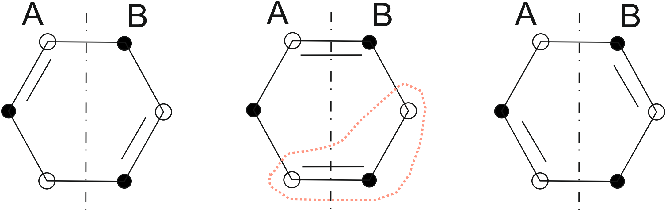
(c)

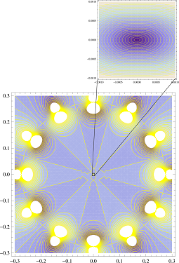
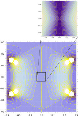
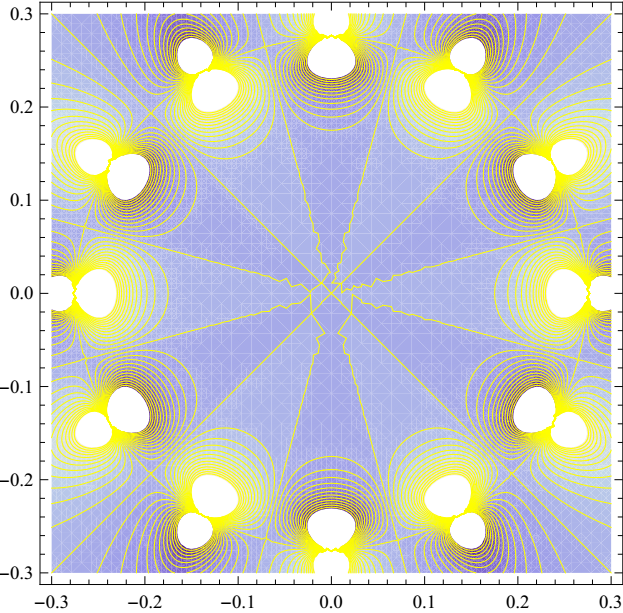
(d)

Figure 1: Models $N=2$ (a), $N=3$ (b). p_z-electrons belonging to triangular sublattices $A$ and $B$ are designated through solid and unfilled circles respectively. An electrically charged exciton is designated by dashed line contour in figure (b). (c) Action of exchange operators on the particle (hole) Hamiltonians $H_{AB(BA)}$ in (III.9) NPCS18-2015GrushevskayaKrylovGaisyonokSerow : (left) Contour plots of sum of original Dirac bands, (middle) of single action of $\left(\Sigma_{rel}^{x}\right)_{BA}$; (right) of action of exchange operators product $\left(\Sigma_{rel}^{x}\right)_{AB}\left(\Sigma_{rel}^{x}\right)_{BA}$ restoring the system. Inset in figure (c, left) demonstrates that the steady state point in the Dirac point $K(K^{\prime})$ is of center type. Inset in figure (c, middle) shows an occurrence of a saddle point. (d) Schematic diagram for braiding Majorana fermions through twisted valley currents, dimer formation and the exchange $\Sigma_{AB(BA)}$. Hole and electron currents are shown in blue and red respectively.

In the model $N=2$ the valley currents are absent due to the fact that all p_z-electrons are pared. Contrary to this, valley currents exist for $N=3$ MyJNPCS2017Vol20 . In contrast to the RVB picture, the stochastic staggered spin flows or identical to them d-density wave states Chakravarty-Laughlin-Morr-Nayak2002 are absent for our model. Their place, as we show further, is occupied by the quantum staggered valley currents of the electric charge carriers with a precessing spin similar to a spin vortex. The spin precession is due to SOC-coupling. Experimentally, such a staggered orbital order (a staggered quadruple ordered phase with distinct orbital polarization on two-sublattices) without lattice distortions has been found in staggered orbital order .

To account translational symmetry, we introduce the phase multiplier $\exp\left\{\imath\Delta\alpha_{\pm,i}\right\}$ to the wave function at site $\pm\delta_{i}$, $i=1,2,3$ in the following form:

$$\exp\left(\pm\imath c_{\pm}(q)({\vec{q}}\cdot{\vec{\delta}_{i}})\right).$$ (III.8)

To eliminate arbitrariness in the choice of phase factors $c_{\pm}$ in (III.8), one needs gauge condition for the phase fields.

III.1 First-order approximation

Let us consider the case of small wave numbers $q$, $q\to 0$. Then, in the first-order approximation, a gauge condition can be chosen as follows. The phases $\alpha_{0}$ and $\alpha_{\pm,k}$, $k=1,\ 2,\ 3$ of the wave functions $\psi_{\mbox{\small p}_{z}}(\vec{r}_{2D})$ and $\psi_{\mbox{\small p}_{z},\pm\vec{\delta}_{k}}(\vec{r}_{2D})$, $k=1,\ 2,\ 3$ respectively are the same for p_z-electrons in the expressions (III.3, III.6) due to (III.8). By virtue of the arbitrariness in the choice of phases at $q\to 0$, the phases in the first-order approximation were chosen the same for all lattice sites.

At power series expansion on a small parameter ${1\over\left<0\right|\hat{v}_{F}\left|0\right>}$ in the right hand side of (II.11), one can neglect the second term for small wave numbers $q$. Then accounting the fact that the mass term $\widetilde{\Sigma_{AB(BA)}\Sigma_{BA(AB)}}$ vanishes in the Dirac point one gets:

$$\vec{\sigma}_{2D}^{BA}\cdot\vec{p}_{AB}\left|\psi_{AB}\right\rangle={E^{(0)}\over\left<0\right|\hat{v}_{F}\left|0\right>}\left|\psi_{AB}\right\rangle.$$ (III.9)

In this case the exchange interaction terms (III.3, III.6) are given by the matrixes with real integrands. It turns out that with such a phases choice for $\psi_{\mbox{\small p}_{z}}(\vec{r}_{2D})$ and $\psi_{\mbox{\small p}_{z},\pm\vec{\delta}_{k}}(\vec{r}_{2D})$, we obtain an imaginary part for the energy $E^{(0)}$ in (III.9) without the mass term myNPCS18-2015 ; myIntJModPhys2016 . The deviations of the first-order approximation from the massless Dirac fermion model Semenoff1984 are of the order of $|q|^{4}$ myJModPhys2014 .

Under the action of $\Sigma_{BA(AB)}$ calculated in the first-order approximation, the Dirac point as a center of circumference trajectories is transformed into a hyperbolic point of a saddle type and subsequent action of $\Sigma_{AB(BA)}$ restores neutral-stability state of the center type in fig. 1c. Therefore, the exchange operator $\Sigma_{AB(BA)}$ plays the role of a braiding operator. Braiding scheme through the formation of a dimer is shown in fig. 1d.

III.2 Second-order approximation

In the second-order approximation the relative phases $\Delta\alpha_{\pm,j}$ in $j$-th primitive cell are different for different cells. Substituting the relative phases (III.8) of particles and holes into (III.3) one gets the exchange interaction operator $\Sigma_{AB}$ in the second order approximation:

$$\Sigma_{AB}={1\over\sqrt{2}(2\pi)^{3}}e^{-\imath(\theta_{k_{A}}-\theta_{K_{B}})}\left(\begin{array}[]{cc}\Sigma_{11}^{AB}&\Sigma_{12}^{AB}\\ \Sigma_{21}^{AB}&\Sigma_{22}^{AB}\end{array}\right),$$ (III.12)

$$\Sigma_{11}^{AB}=I_{11}\sqrt{2}\left\{\sum_{j}e^{-\imath c_{-}(\vec{q})(\vec{q}\cdot\vec{\delta}_{j})}\exp\{\imath[\vec{K}^{j}_{A}-\vec{q}]\cdot\vec{\delta}_{j}\}\right\},$$ (III.13)

$$\Sigma_{12}^{AB}=\left\{\sum_{j}\left(I_{12}+I_{11}e^{-\imath c_{-}(\vec{q})(\vec{q}\cdot\vec{\delta}_{j})}\right)\exp\{\imath[\vec{K}^{j}_{A}-\vec{q}]\cdot\vec{\delta}_{j}\}\right\},$$ (III.14)

$$\Sigma_{21}^{AB}=\left\{\sum_{j}\left(I_{21}e^{\imath(c_{+}(\vec{q})-c_{-}(\vec{q}))(\vec{q}\cdot\vec{\delta}_{j})}+I_{11}e^{-\imath c_{-}(\vec{q})(\vec{q}\cdot\vec{\delta}_{j})}\right)\exp\{\imath[\vec{K}^{j}_{A}-\vec{q}]\cdot\vec{\delta}_{j}\}\right\},$$ (III.15)

$$\Sigma_{22}^{AB}={1\over\sqrt{2}}\left\{\sum_{j}\left(I_{22}e^{\imath c_{+}(\vec{q})(\vec{q}\cdot\vec{\delta}_{j})}+I_{12}+I_{21}e^{\imath(c_{+}(\vec{q})-c_{-}(\vec{q}))(\vec{q}\cdot\vec{\delta}_{j})}+I_{11}e^{-\imath c_{-}(\vec{q}))(\vec{q}\cdot\vec{\delta}_{j})}\right)\exp\{\imath[\vec{K}^{j}_{A}-\vec{q}]\cdot\vec{\delta}_{j}\}\right\},$$ (III.16)

$$I_{11}=\int V(\vec{r})\psi^{(0)}_{\mbox{\small p}_{z}}{\psi^{*}}^{(0)}_{\mbox{\small p}_{z}-\vec{\delta}_{j}}\ d\vec{r},\ \ I_{12}=\int V(\vec{r})\psi^{(0)}_{\mbox{\small p}_{z}}{\psi^{*}}^{(0)}_{\mbox{\small p}_{z}}\ d\vec{r},$$ (III.17)

$$I_{21}=\int V(\vec{r})\psi_{\mbox{\small p}_{z}+\vec{\delta}_{j}}{\psi^{*}}_{\mbox{\small p}_{z}-\vec{\delta}_{j}}\ d\vec{r},\ \ I_{22}=\int V(\vec{r})\psi_{\mbox{\small p}_{z}+\vec{\delta}_{j}}{\psi^{*}}_{\mbox{\small p}_{z}}\ d\vec{r}\ ;$$ (III.18)

and similar formulas for $\Sigma_{BA}$. Now, neglecting the mass term, we can find the solution of the equation (II.11) by the successive approximation technique as:

$$\vec{\sigma}_{2D}^{BA}(\alpha_{\pm,i})\cdot\vec{p}_{AB}\left|\psi_{AB}(\alpha_{\pm,i})\right\rangle+{E^{(0)}\left(\Delta\Sigma+\left[\Sigma_{AB},\Sigma_{BA}\right]\right)\over\left<0|\hat{v}_{F}|0\right>^{2}}\left|\psi_{AB}(\alpha_{\pm,i})\right\rangle={E^{(1)}\over\hat{v}_{F}}\left|\psi_{AB}(\alpha_{\pm,i})\right\rangle.$$

(III.19)

Here $\Delta\Sigma,\ \Sigma_{AB},\Sigma_{BA}$ are determined by the expressions (III.12–III.18).

Eigenvalues $E^{(1)}_{i},\ i=1,\ 2$ of (III.19) are functions of $c_{\pm}$. The gauge condition is imposed as a requirement on the absence of imaginary parts in eigenvalues $E^{(1)}_{i},\ i=1,\ 2$ of (III.19). This condition can be written as a system of two equations of the form

$$\Im m(E^{(1)}_{i})=0,\ i=1,\ 2.$$ (III.20)

Direct solution of this system turns out to be unstable for some specific points in the momentum space. Instead, for every point in the momentum space we use a minimization procedure with the price function $f(c_{+},c_{-})=\left|\Im m\ E^{(1)}_{1}\right|+\left|\Im m\ E^{(1)}_{2}\right|$. Its absolute minimum evidently coincides with the solution of the system (III.20).

The phase factors $c_{\pm}$ (III.8) entering (III.19) periodically change their values on the polar angle $\phi$ with the period $\pi$ in fig. 2, and hence our model describes 2D $\mathbb{Z}_{2}$-topological insulators Zak-phase1989 ; Short-Course-on-Topological-Insulators ; Wilczek-Zee1984PRL ; Topological-Dirac-nodal-lines2017NatCom . The gauge fields $c_{\pm}$ hold hexagonal symmetry near the Dirac point $K(K^{\prime})$ and are rotated on $60^{\circ}$ with respect to each other in figs. 2a, d. At high momenta the gauge field $c_{+}$ changes symmetry to octagonal one in $\vec{q}$-space as figs. 2c, b demonstrate. The behaviour of the phases $\{c_{+},c_{-}\}$ in figs. 2a, d is the same and hence they describe the same gauge field. The gauge field fluctuates strongly and is characterized by the hexagonal symmetry near the Dirac point $K(K^{\prime})$ due to phase entanglement $\{c_{+},c_{-}\}$. A core of vortex is observed in figs. 2a, d so that $c_{+}$, $c_{-}$ fluctuate least of all at the boundary of six identical sectors of the circle. With the increase of the excitation energy $E(q)$, the value of the gauge field begins to increase only in one of three pairs of sectors of the circle in figs. 2a, d.

With the increasing $E(q)$, the amplitude of the fluctuations decreases and 2D $\mathbb{Z}_{2}$-topological phase is originated. The phases $\{c_{+},c_{-}\}$ become two different gauge fields as it is shown in figs. 2c, f; and, hence, the gauge field is deconfined. The phase $c_{+}$ changes sharply its sign four times due to the eight-fold Dirac cone for the deconfined quasiparticle state at large excitation energy $E(q)$ (high momentum $q$) in fig. 2g. The phases $c_{+}$, $c_{-}$ start to fluctuate strongly with the decrease of the value $E(q)$ as, for example, $c_{-}(\phi)$ dependency demonstrates in fig. 2h.

(a)                                            (b)                                            (c)

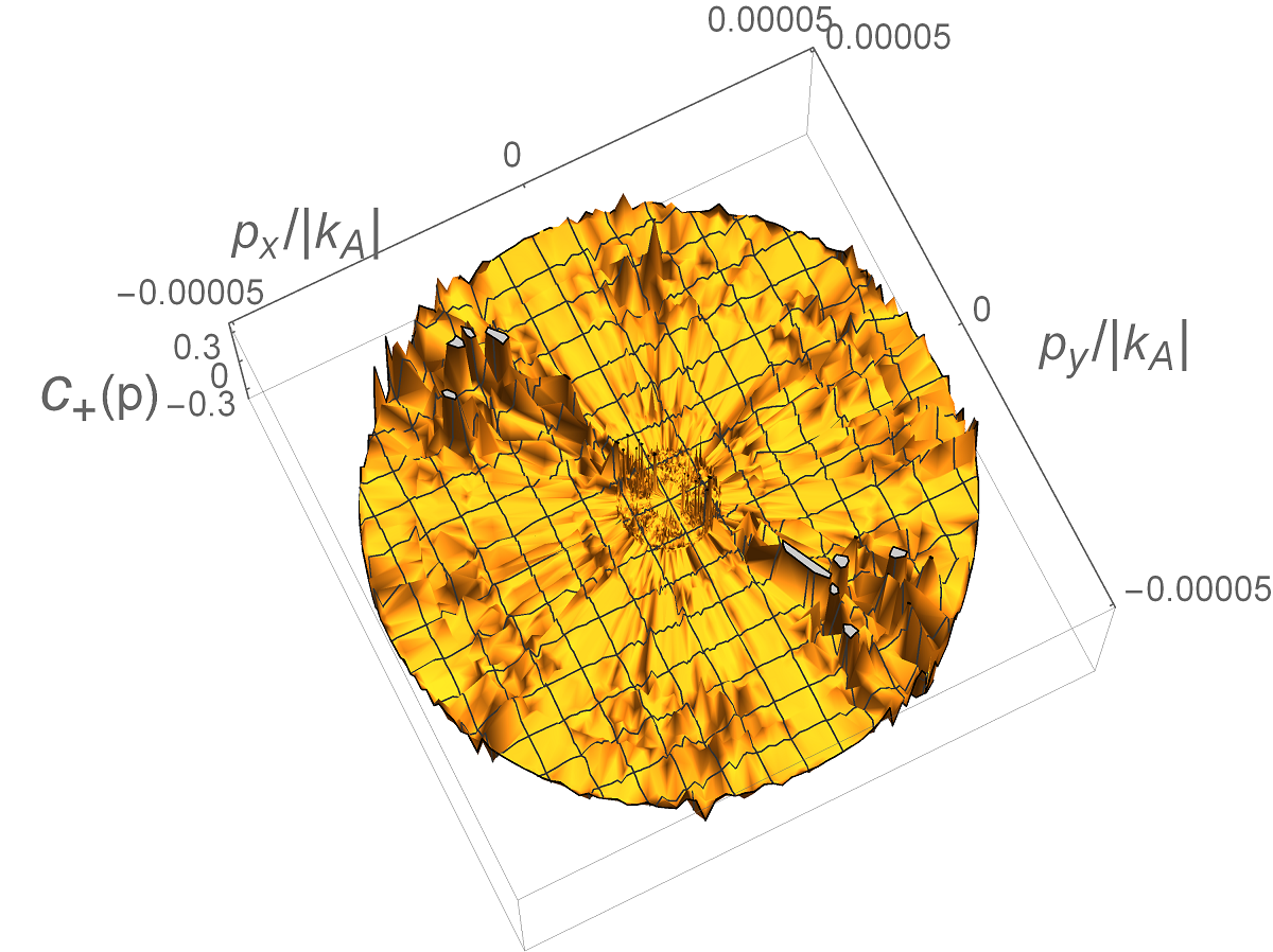
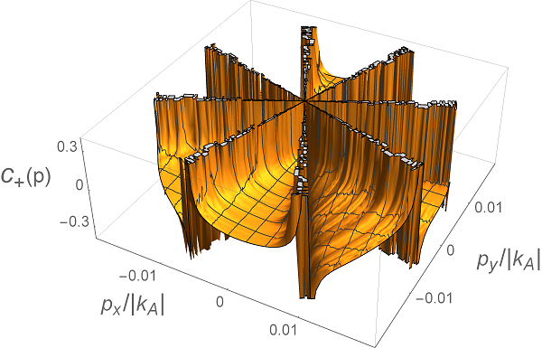
(d)                                            (e)                                            (f)

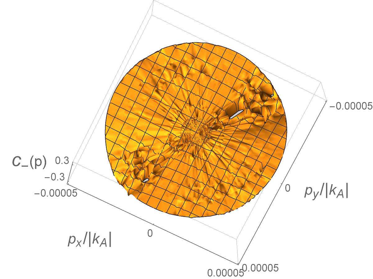
(g)                                            (h)
         

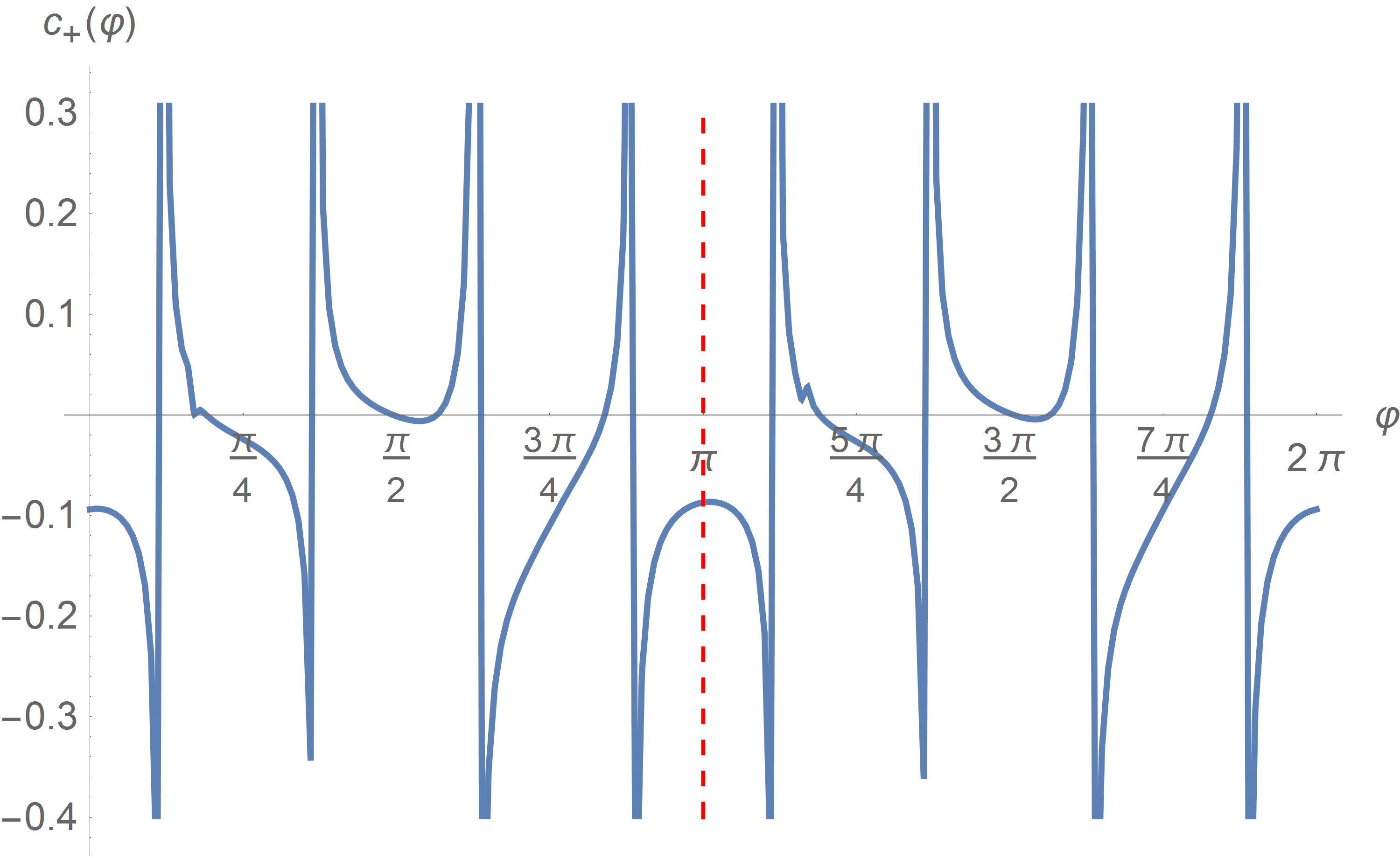
Figure 2: Scenario of $\mathbb{Z}_{2}$ topological gapless-phase emerging through deconfinement. (a, d) Zero-value gauge field $\{c_{+},c_{-}\}$ in the Dirac point $K(K^{\prime})$ and its $\epsilon$-neighbourhood, $\epsilon\sim 2\cdot 10^{-8}$ and emergent hexagonal symmetry of the field in the energy range $\sim 10^{-7}$. (b, e) Origin of 2D $\mathbb{Z}_{2}$-topological semimetal at energies $\sim 5\cdot 10^{-7}-10^{-5}$. (c, f) Deconfinement of the gauge field $\{c_{+},c_{-}\}$ by SOC at the energies $\sim 10^{-2}$. Angle dependencies of phases $c_{+}$ and $c_{-}$ entering in the exchange matrix at different excitation energies $E(q)$: $0.02$ (g) and $5\cdot 10^{-5}$ (h) respectively.

III.3 Dichroism of the Dirac bands, deconfinement, nodal lines and drumhead surface states

A helicoidal spin-valley-orbit texture of the Majorana bands (III.19) shown in fig. 3 is originated in the $\sigma-p_{z}$ coupling between the orbital momentum $p_{z}$ of $\pi$-electron and the $\pi$-electron spin $\sigma$ oriented along two directions: tangent $\vec{n}_{\phi}$ and radial $\vec{n}_{r}$. One can see that the Dirac point hosts such a ”defect”, as a core of vortex in the in fig. 3b-d. This topological defect is a Majorana zero-energy mode. Multiple vortices structure of these bands is visualized in the form of concentric circles of varying degrees of helicoidality and different widths. The spin-valley-orbit texture varies in both space and time. Dichroism of ARPES spectra is a manifestation of the $\pi$-electron-orbit pseudo-precession in inset to fig. 3d. Since the pseudo-Majorana modes are simultaneously their antimodes, Majorana sinks (vortex cores) are simultaneously Majorana sources (antivortex anticores). Sinks and sources locating at the same place braid particles and holes into Majorana fermions.

(a)                                             (b)                                             (c)

(d)                                                                                        (e)

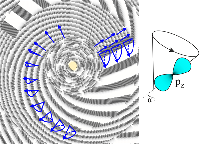
Figure 3: Band structure with the Majorana zero-energy modes in the Dirac cone apexes for the semimetal model $N=3$ (a), their spin-orbit texture of the scale: $q/|K_{A}|\sim 5\times 10^{-7}$ (b), 0.01 (c), 0.002 (d) in contour plots (b–d); and a model vortex of the precessing orbitals in inset to figure (d). The angle $\alpha$, $0\leq\alpha\leq\pi/2$ is the precession angle of p_z-orbital. (e) Sketch of ARPES mappings on a Majorana band structure for an orthorombic T_d-MoTe₂ (blue and violet lines) and PbTaSe₂ (red lines). Insets are (left) photoemission spectral intensity map of T_d-MoTe₂ at binding energy $E_{B}=0.0,\ 0.025$ eV Signature-of-type-II-Weyl-semimetal2017NatCom and (right) ARPES spectra of PbTaSe₂ taken along $\overline{M}-\overline{K}-\overline{\Gamma}$ with 64-eV photons NatCommunic7-2016Bian .

Deconfinement which splits the four-fold particle (hole) Dirac cone, should lead to the divergence of the locations of sinks and sources. Meanwhile, a nodal ring $NL_{D}$, an image of which is schematically presented in fig. 3e, separates the region of eightfold splitting of the Dirac cone in fig. 3a. The left- and right-hand $\pi$(p_z) electrons possess relativistic total angular momentum $J=3/2$ due to SOC after the deconfinement. The emergent tilted Dirac cones which have been introduced earlier as tilted Dirac cone replicas in myNPCS2013 break the vortices in fig. 3c, d. Vortex current lines pass from one vortex cores to others. The connections of different vortices form an infinite number of Fermi arcs which link divergent Majorana sinks and anti-sinks. Hence, together with the nodal ring $NL_{D}$, four more pairs of Weil nodal lines are formed.

Divergence of sinks and sources transforms the brainding Majorana excitations into another type of massless fermions in such a way that their vacuum core and anticore states become uncorrelated. Thus, before the deconfinement, the secondary quantized wave function always describes a fermionic state, entangled with a particle–hole pair, whereas after the deconfinement the non-correlated vacuum spin up and down states lead to $SU(2)\otimes SU(2)\cong O(4)$ symmetry for the system MyLambert .

For certain crystal groups describing nodal-line semimetals quasiparticles are eight-fold degenerate fermions with $SU(2)$ holonomy of wave functions (Wilson loop Alexandradinata-2014 ; Alexandradinata-2016 )PhysRevLett116-2016Wieder ; Science353-2016Bradlyn . Thus, the Majorana particles decay into a continuous set of Weyl nodes and a number of quasiparticle excitations in such a decay channel does not change. Since the number of particles remains unchanged, the Luttinger theorem still holds. Indeed, the hole (particle) pockets are observed in ARPES-spectra for nodal-line TIs PhysRevX6-2016Muechler ; Nature527-2015Soluyanov . In the $q^{4}$ model (III.9) with dumping $\gamma$, nodal lines decay into a discrete set of Wey nodes mySymmetry2016 .

Now, we can predict features of band structures, which should be observed in ARPES of topological SMs. Removing the degeneracy of zero-energy Majorana mode leading also to divergence (unbraiding) of Majorana sinks and sources, yields as well to two additional nodal rings $NL_{1}$ and $NL_{2}$ as it is shown in fig. 3e. $NL_{D},\ NL_{i}$, $i=1,2$ form a contour of drumhead-like states dispersing inwards with respect to $K$. The three nodal rings and the drumhead-like surface states in ARPES spectrum shown in fig. 3e are features of ARPES spectra in the right inset to this figure for superconductor PbTaSe₂ NatCommunic7-2016Bian . At the place of touching of $NL_{1}$ and $NL_{2}$ Majorana sink and source form a Dirac-like band, orthogonal to the origin Dirac band as it is shown in fig. 3e. Such a band structure shown in left inset to fig. 3e is a feature of type-II topological Weyl SMs as WTe₂, MoTe₂ JETPLetters103-2016Zyuzin ; PhysRevX6-2016Muechler ; Signature-of-type-II-Weyl-semimetal2017NatCom ; Nature527-2015Soluyanov .

So, the spin valley-currents coupling, which is small on the energy, turns out to be topologically protected by emergent vortices.

III.4 Majorana dynamical mass operator and chiral anomaly

Eigenvalues of the mass operator $\widetilde{\Sigma_{AB}\Sigma_{BA}}$ (II.5) are represented in fig. 4. These values are the dynamic masses of particle and hole components of the Majorana state. Since the eigenvalues are equal to zero in the Dirac points $K,\ K^{\prime}$ Majorana zero energy modes exist in our model.

Let us prove that the chirality of zero-energy modes is preserved in the Dirac points. Within the approximation of zero gauge-phases (the first-order approximation) $c_{\pm}(\vec{k})$, and respectively zero-valued gauge fields, the eigenvalues of the mass operator differ by two orders of magnitude from each other outside of the Dirac point, as one can see from the comparison of particle and hole masses in fig. 4a,b. Since the mass operator is not diagonal in the energy representation of the massless Hamiltonian $H_{0}$, the masses of Majorana fermions are obtained by mixing particle and hole states. The density of 2D-states (DOS) holds the van Hove singularity Bassani1975 , because DOS is divergent in the Dirac point. Since a hyperbolic point (saddle) is a feature of the dependence of mass on momentum in fig. 4a, b this singularity remains after including the mass term. Therefore, particle and hole densities are concentrated at the energy $E=0$, that leads to particle–hole annihilation. Since the mass term is alternating in one point, the chirality is preserved for the Majorana zero-energy modes only. In the first-order approximation there is no such a neighborhood of the Dirac point, where the mass term takes zero values and hence the Dirac bands are not chiral everewhere except of the Dirac points. Thus, dichroism of the bands can not be described in the zero-gauge-field approximation. In what follows we show that dichroism can be observed in the second-order approximation.

The comparison of particle and hole masses in fig. 4a, c demonstrates that in the second-order approximation of non-zero gauge fields $c_{\pm}(\vec{q})$, qualitatively the same momentum dependence remains for one of the mass operator eigenvalues. The dependence of the mass-term second eigenvalue upon the momentum in fig. 4d exhibits a singular alternating behaviour and gets a zero values in the vicinity of the Dirac point. It means that chirality is preserved not only in the Dirac point but in the Dirac band as well. Meanwhile, the dichroism is observed outside the Dirac point but only one of two right- or left-hand Majorana modes remains chiral. The appearance of the mass term peak in fig. 4d leads to divergence of DOS at some another value of the energy $E$, that makes the particle and hole densities spatially separated from to each other. As a result, there exist non-zero energy Majorana modes in the model $N=3$ without particle–hole annihilation.

(a)                                    (b)                                    (c)                                     (d)

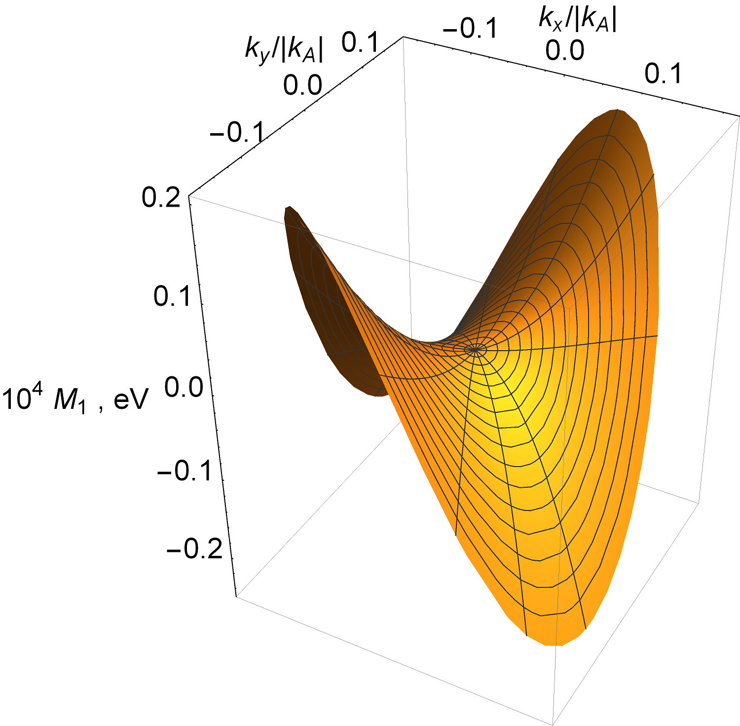
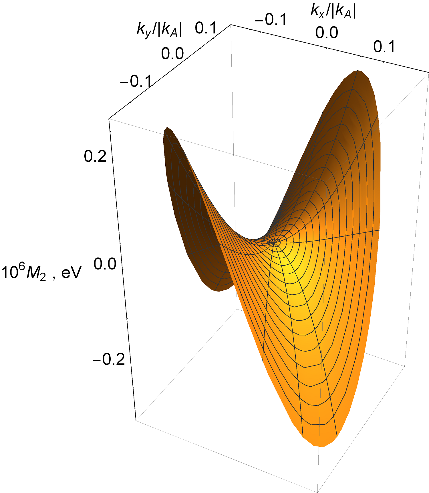
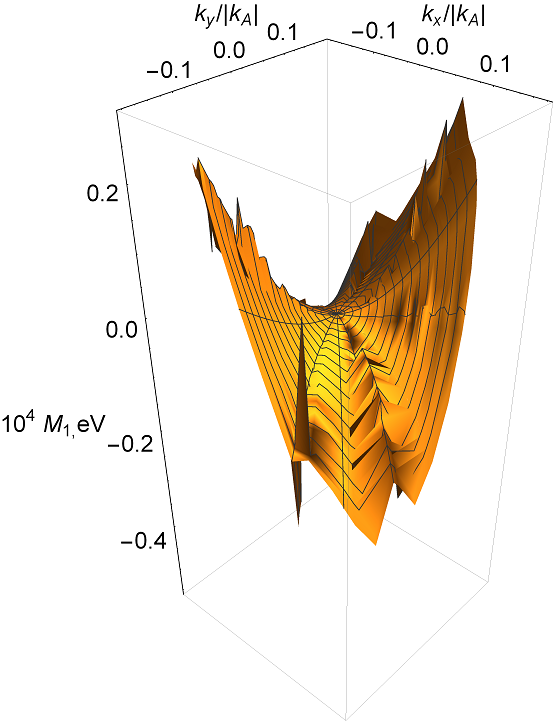
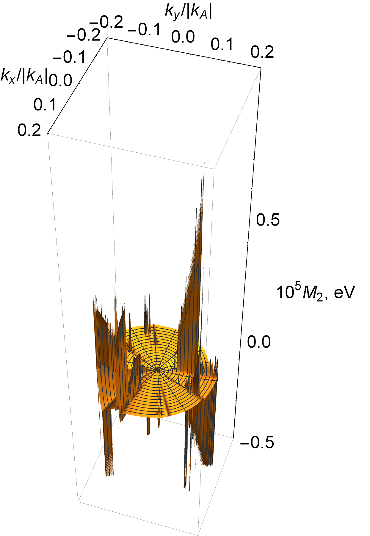
Figure 4: Eigenvalues of the mass operator in approximations of zero (a, b) and non-zero (c, d) gauge fields. (a, c) - for particles (holes), (b, d) - for holes (particles).

Values of spectral weight (spectral function) $A(q,\omega)$ are much higher for a heavy particle than for the light one. Accordingly, the dielectric permeability of the system of heavy particles is very small compared with those of the system of light ones Kraft-Ropke . Hence, low-intensive Fermi arcs of the heavy particle (hole) components of Majorana states augment much more intensive Fermi arcs of the light ones up to Fermi particle(hole) pockets. Therefore, the Luttinger theorem is not violated in our approach. Moreover, the examples of the narrow-gap chalcogenide Pb$Me$, $Me=$ Te, Se, S being graphene three-dimensional analogue Comput-Mater-Sci2005 ; Falkovsky2008PhysUspekhi and of doped Mott insulator La_2-xSr_xTiO₃ Tokura1993PRL appear to take the heavy mass route.

So, the construction and simulation of the mass operator in the topological SM theory point to the main difference of the chiral lattice theory of particle–hole pairs from the theory of Majorana fermions. A Majorana mass term $\cal{L}_{M}$ for left-hand $\psi_{L}$ and right-hand $\psi_{R}$ Majorana wave functions reads ${\cal L}_{M}\propto\left(\psi_{L}\right)^{T}\gamma_{0}\psi_{L}+\left(\psi^{*}_{L}\right)^{T}\gamma_{0}\psi^{*}_{L}$ owing to $\psi_{R}=\psi^{*}_{L}$ and, hence, chirality of the Majorana theory is broken everywhere except of zero-energy states PhysicsEMajorana-2014Wilczek . Contrary to that in our Majorana-like theory, the second eigenvalue of the mass term equals to zero in the vicinity of the Dirac point and therefore the chirality breaks for only one constituent of a particle-hole pair. The violation of the law of conservation of topological charge in the form of weak imbalance in the number of topological charges of the opposite signs is a feature of our theory. It is called a chiral anomaly.

IV Charge carrier transport in the model $N=3$

An equation with accounting of electron-photon interactions in the semimetal can be obtained from (II.11) by ordinary use of the canonical momentum:

$$\left[c\vec{\sigma}_{2D}^{BA}\cdot\left(\vec{p}_{AB}-{e\over c}\vec{A}\right)-\widetilde{\Sigma_{AB}\Sigma_{BA}}\left(\vec{p}_{AB}-e\vec{A}/c\right)\right]\widehat{\tilde{\chi}^{\dagger}_{+\sigma_{{}_{B}}}}(\vec{r})\left|0,-\sigma\right>=cE_{qu}(p)\widehat{\tilde{\chi}^{\dagger}_{+\sigma_{{}_{B}}}}(\vec{r})\left|0,-\sigma\right>,$$ (IV.1)

$$\widetilde{\Sigma_{AB}\Sigma_{BA}}\left(\vec{p}_{AB}-e\vec{A}/c\right)=\widetilde{\Sigma_{AB}\Sigma_{BA}}(0)+\sum_{i}\left.{d\widetilde{\Sigma_{AB}\Sigma_{BA}}\over dp_{i}^{\prime}}\right|_{p_{i}^{\prime}=0}\left(p_{i}^{AB}-{e\over c}A_{i}\right)$$

$$+{1\over 2}\sum_{i,j}\left.{d^{2}\widetilde{\Sigma_{AB}\Sigma_{BA}}\over dp_{i}^{\prime}dp_{j}^{\prime}}\right|_{p_{i}^{\prime},\ p_{j}^{\prime}=0}\left(p_{i}^{AB}-{e\over c}A_{i}\right)\,\left(p_{j}^{AB}-{e\over c}A_{j}\right)+\ldots.$$ (IV.2)

In what follows, we omit the cumbersome designation ”$AB$” if this does not lead to the lack of sense.

Now, taking into account the equations (IV.1) and (IV.2)), one can find the quasi-relativistic current Davydov of charge carriers in SM as:

$$j_{i}^{SM}=c^{-1}j_{i},$$

$$j_{i}=e\chi^{\dagger}_{+\sigma_{{}_{B}}}(x^{+})v^{i}_{x^{+}x^{-}}\chi_{+\sigma_{{}_{B}}}(x^{-})-{e^{2}A_{i}\over c\,\widetilde{\Sigma_{AB}\Sigma_{BA}}(\vec{p}_{AB}-e\vec{A}/c)}\chi_{+\sigma_{{}_{B}}}^{\dagger}(x^{+})\chi_{+\sigma_{{}_{B}}}(x^{-})$$

$$+{e\hbar\over 2\widetilde{\Sigma_{AB}\Sigma_{BA}}(\vec{p}_{AB}-e\vec{A}/c)}\left[\vec{\nabla}\times\chi_{+\sigma_{{}_{B}}}^{\dagger}(x^{+})\vec{\sigma}\chi_{+\sigma_{{}_{B}}}(x^{-})\right]_{i}.$$ (IV.3)

Here

$$x^{\pm}=x\pm\epsilon,\ x=\{\vec{r},\ t_{0}\},\ t_{0}=0,\ \epsilon\to 0;$$ (IV.4)

$\vec{v}$ is the velocity operator determined by a derivative of the Hamiltonian (IV.1). It worth to remark that in accord with (IV.4) the current is obtained from the quantity dependent upon two points $x^{\pm}$, with subsequent performing the limit $\epsilon\to 0$. 2D-rotor in the series expansion (IV.3) can be presented in the form

$$\nabla\times\chi_{+\sigma_{{}_{B}}}^{\dagger}\vec{\sigma}\chi_{+\sigma_{{}_{B}}}\sim\sum_{i=1}^{2}\left[\nabla\times\chi_{+\sigma_{{}_{B}}}^{\dagger}\vec{\sigma}\chi_{+\sigma_{{}_{B}}}\right]_{i}\vec{e}_{i}=\left[{\partial\over\partial y}\vec{e}_{1}-{\partial\over\partial x}\vec{e}_{2}\right]\chi_{+\sigma_{{}_{B}}}^{\dagger}\sigma_{z}\chi_{+\sigma_{{}_{B}}}$$ (IV.5)

where $\vec{e}_{i}$, $i=1,\,2$ are unit vectors along the coordinate axis directions. The substitution of (IV.5) into (IV.3) gives

$$\begin{split}j_{i}=j_{i}^{Ohm}+j_{i}^{Zitterbew}+j_{i}^{spin-orbit},\\ j_{i}^{Ohm}=e\chi^{\dagger}_{+\sigma_{{}_{B}}}(x^{+})v^{i}_{x^{+}x^{-}}\chi_{+\sigma_{{}_{B}}}(x^{-}),\\ j_{i}^{Zitterbew}=-{e^{2}A_{i}\over c\,\widetilde{\Sigma_{AB}\Sigma_{BA}}(\vec{p}_{AB}-e\vec{A}/c)}\chi_{+\sigma_{{}_{B}}}^{\dagger}\chi_{+\sigma_{{}_{B}}},\\ j_{2(1)}^{spin-orbit}=(-1)^{1(2)}{\imath e\over 2}v^{1(2)}_{x^{+}x^{-}}\chi_{+\sigma_{{}_{B}}}^{\dagger}\sigma_{z}\chi_{+\sigma_{{}_{B}}}.\end{split}$$ (IV.6)

Terms $j_{i}^{Ohm},\ j_{i}^{Zitterbew},\ j_{i}^{spin-orbit}$ in (IV.6) describe ohmic contribution which satisfies the Ohm law and contributions of the polarization and magneto-electric effects respectively.

Now, calculating the currents (IV.6) one can find the Ohmic conductivity (equation S.77 in Supplementary Information), the polarization and magneto-electric contributions to it (equations S.81 and S.84 in Supplementary Information) through the scalar product $(\cdot\,,\,\cdot)$ of the vectors $M\vec{v}^{i}(p)$ and $N\vec{v}^{i}(p)$, $i=x,\ y$ as

$$\sigma_{ii}^{Ohm}(\omega^{-+},\ k)={\imath e^{2}\bar{\beta}\over(2\pi c)^{2}}\ \mbox{Tr}\ \int\left(1-\widetilde{\Sigma_{AB}\Sigma_{BA}}(\vec{p}_{AB}-e\vec{A}/c){d^{2}\widetilde{\Sigma_{AB}\Sigma_{BA}}\over dp_{i}^{AB}dp_{i}^{AB}}(0)\right)\left(M\vec{v}^{i}(p)\,,\,N\vec{v}^{i}(p)\right)\,d(\bar{\beta}\vec{p}),\ \ \$$ (IV.7)

$$\sigma_{ll}^{Zitterbew}(\omega^{-+},\ k)={\imath e^{2}\bar{\beta}\over(2\pi c)^{2}}\mbox{Tr }\ \int{\widetilde{\Sigma_{AB}\Sigma_{BA}}(\vec{p}_{AB}-e\vec{A}/c)\over 2}\sum_{i=1}^{2}{d^{2}\widetilde{\Sigma_{AB}\Sigma_{BA}}\over dp_{i}^{2}}\left(M\vec{v}^{i}(p)\,,\,N\vec{v}^{i}(p)\right)\,d(\bar{\beta}\vec{p}),\ \ \$$ (IV.8)

$$\sigma_{12(21)}^{spin-orbit}(\omega^{-+},\ k)=(-1)^{1(2)}{\imath\over 2}{\imath e^{2}\bar{\beta}\over(2\pi c)^{2}}\mbox{Tr }\ \int{\widetilde{\Sigma_{AB}\Sigma_{BA}}(\vec{p}_{AB}-e\vec{A}/c)}{d^{2}\widetilde{\Sigma_{AB}\Sigma_{BA}}\over dp_{1(2)}dp_{2(1)}}(0)$$

$$\times\left(M\vec{v}\,^{1(2)}(p)\,,\,N\vec{v}\,^{1(2)}(p)\right)\sigma_{z}d(\bar{\beta}\vec{p}).$$ (IV.9)

where matrices $M,\ N$ are given by the following expressions:

$$\begin{split}M={f[\beta((H(p^{+})-\mu)/\hbar)]-f[\beta(H^{\dagger}(-p^{-})-\mu/\hbar)]\over\beta(z^{-+})-\beta(H(p^{+})/\hbar)+\beta(H^{\dagger}(-p^{-})/\hbar)},\ N={\delta\left(\hbar\omega^{-+}+\mu^{-+}\right)\over\hbar(z^{-+}+\omega^{e}(\hat{p}^{+})-\omega^{h}(-\hat{p}^{-}))\bar{\beta}}.\end{split}$$ (IV.10)

Here $f$ is a Fermi – Dirac distribution, $\beta$ is an inverse temperature. In the diagonal Hamiltonian representation, the trace in (IV.7 – IV.9) can be easily carried out, for example, as

$$\left(\mbox{Tr}\ M\vec{v}\,^{x}_{AB}\,,\,N\vec{v}\,^{y}_{AB}\right)=\mbox{Tr}\ \left(M\vec{v}\,^{x}_{AB}\,,\,N\vec{v}\,^{y}_{AB}\right)=(\vec{e}_{x},\vec{e}_{y})\sum_{i,k,l,m=1}^{2}{v^{\dagger}}^{x,AB}_{ik}M^{\dagger}_{kl}N_{lm}v^{y,AB}_{mi}$$

$$=(\vec{e}_{x},\vec{e}_{y})\sum_{i,\,k=1}^{2}{v^{\dagger}}^{x,AB}_{ik}M^{\dagger}_{kk}N_{kk}v^{y,AB}_{ki}$$ (IV.11)

because matrices $M_{kl},N_{kl}$ depending on the diagonal matrix $H_{AB}$ are diagonal ones.

Since there exists the change $-H(p)\to H^{\dagger}(-p)$, for every band $a$ ($a=1,\,2$), it is possible to introduce Hamiltonians of a quasi-particle $H_{0}^{a}$, $\mathop{H_{0}^{a}}^{\dagger}$ with eigenvalues $E^{e}_{a}$, $E^{h}_{a}$ and respectively to quantize $M$ and $N$ (IV.10) as

$$M^{\dagger}=\left\{M^{\dagger}_{ab}\right\},\ M^{\dagger}_{ab}={f[\bar{\beta}(H_{0}^{a}(p^{+})-\mu)]-f[\bar{\beta}(\mathop{H_{0}^{b}}^{\dagger}(-p^{-})-\mu)]\over\bar{\beta}\hbar z^{-+}-\bar{\beta}H_{0}^{a}(p^{+})+\bar{\beta}\mathop{H_{0}^{b}}^{\dagger}(-p^{-})};$$ (IV.12)

$$N^{\dagger}=\left\{N^{\dagger}_{ab}\right\},\ \ N^{\dagger}_{ab}={\delta\left(\hbar\omega^{-+}+\mu^{-+}\right)\over(\hbar\omega+H_{0}^{b}(p^{+})-\mathop{H_{0}^{a}}^{\dagger}(-p^{-}))\bar{\beta}}.$$ (IV.13)

As a result, the expression (IV.11) can be rewritten in the form

$$\left(\mbox{Tr}\ Mv^{x}_{AB}\,,\,Nv^{y}_{AB}\right)=(\vec{e}_{x},\vec{e}_{y})\sum_{a=1}^{2}\left(v^{x,AB}_{aa}M^{\dagger}_{aa}N_{aa}v^{y,AB}_{aa}+v^{x,AB}_{ab}M^{\dagger}_{ba}N_{ab}v^{y,AB}_{ba}\right),\ a\neq b.$$ (IV.14)

After substitution of (IV.12 – IV.14) into (IV.7), we express, for example, the Ohmic contribution to conductivity as

$$\sigma_{ij}^{Ohm}(\omega^{-+},\ k)={\imath e^{2}\bar{\beta}\over(2\pi c)^{2}}\int(\vec{e}_{i},\vec{e}_{j})\left(1-\widetilde{\Sigma_{AB}\Sigma_{BA}}(\vec{p}_{AB}-e\vec{A}/c){d^{2}\widetilde{\Sigma_{AB}\Sigma_{BA}}\over dp_{i}^{AB}dp_{j}^{AB}}(0)\right)$$

$$\times\sum_{a=1}^{2}\left\{{v^{\dagger}}^{i}_{aa}(p,\ k){f[\bar{\beta}(H_{0}^{a}(p^{+})-\mu)]-f[\bar{\beta}(\mathop{H_{0}^{a}}^{\dagger}(-p^{-})-\mu)]\over\bar{\beta}\hbar z^{-+}-\bar{\beta}H_{0}^{a}(p^{+})+\bar{\beta}\mathop{H_{0}^{a}}^{\dagger}(-p^{-})}v^{j}_{aa}(p,\ k)\right.$$

$$\times{1\over(\hbar\omega^{-+}+H_{0}^{a}(p^{+})-\mathop{H_{0}^{a}}^{\dagger}(-p^{-}))\bar{\beta}}+{f[\bar{\beta}(H_{0}^{a}(p^{-})-\mu)]-f[\bar{\beta}(\mathop{H_{0}^{b}}^{\dagger}(-p^{+})-\mu)]\over\bar{\beta}\hbar z^{-+}-\bar{\beta}H_{0}^{a}(p^{+})+\bar{\beta}\mathop{H_{0}^{b}}^{\dagger}(-p^{-})}$$

$$\left.\times{{v^{\dagger}}^{i}_{ab}(p,\ k)v^{j}_{ba}(p,\ k)\over(\hbar\omega^{-+}+H_{0}^{b}(p^{+})-\mathop{H_{0}^{a}}^{\dagger}(-p^{-}))\bar{\beta}}\right\}\ d(\bar{\beta}\vec{p})\delta\left(\hbar\omega^{-+}+\mu^{-+}\right),\ a\neq b;\ \ a,b=1,2.$$ (IV.15)

IV.1 Approximation of the degenerate Dirac cone

In the case of degeneration $E^{e}_{1,\,2}(p)\approx\mp cv_{F}\hbar p$, $E^{h}_{1,\,2}(p)\approx\pm cv_{F}\hbar p$. Since $E_{a}^{e}(p)=E_{a}^{h}(-p)$, using calculus in section II of Supplementary Information and neglecting the dynamic mass correction, we get the intraband-transition contribution $\sigma_{aa,\,ij}^{Ohm}$ to conductivity due to the transitions in the same band:

$$\sigma_{aa,\,ij}^{Ohm}(\omega,\ k)={\imath e^{2}\over c^{2}(2\pi)^{2}}{\bar{\beta}}\int v^{i}_{aa}(p,\ k){f[\bar{\beta}(H_{0}^{a}(p^{-})-\mu)]-f[\bar{\beta}(\mathop{H_{0}^{a}}^{\dagger}(-p^{+})-\mu)]\over\bar{\beta}\hbar z-\bar{\beta}H_{0}^{a}(p^{-})+\bar{\beta}\mathop{H_{0}^{a}}^{\dagger}(-p^{+})}v^{j}_{aa}(p,\ k)$$

$$\times{1\over(\hbar\omega-\mathop{H_{0}^{a}}^{\dagger}(-p^{+})+H_{0}^{a}(p^{-}))\bar{\beta}}\ d(\bar{\beta}\vec{p})=-{\imath e^{2}\over c^{2}(2\pi)^{2}}$$

$$\times\int{\omega(k)v^{i}_{aa}(p,\ k)v^{j}_{aa}(p,\ k)\partial f[\bar{\beta}(E_{a}(p)-\mu)]/\partial E_{a}(p)\over(\hbar z\hbar\omega-\omega(k)\hbar\omega+\hbar z\omega(k)-\omega^{2}(k))}\ d\vec{p},\quad i,j\in\{x,y\}.$$ (IV.16)

Here $E_{a}(p)=E_{a}^{e}(p)=E_{a}^{h}(-p)$. Let us make the change $\omega(k)\to c\tilde{\omega}(k)$, and account for the existence of $\delta(\hbar(z^{-}-z^{+})-\hbar z)$. Then calculating (IV.16) one gets:

$$\sigma_{aa,\,ij}^{Ohm}(\omega,\ k)=-{\imath e^{2}\over(2\pi)^{2}}$$

$$\times\int{\tilde{\omega}(k)\tilde{v}^{i}_{aa}(p,\ k)\tilde{v}^{j}_{aa}(p,\ k)\partial f[(\epsilon_{a}(p)-\mu)/T]/\partial\epsilon_{a}(p)\over(\hbar z_{12}\omega-c\tilde{\omega}(k)\hbar\omega+c\hbar z\tilde{\omega}(k)-c^{2}\tilde{\omega}^{2}(k))}\ d\vec{p},\quad i,j\in\{x,y\}.$$ (IV.17)

where $\epsilon_{a}=E_{a}/c$, $\tilde{v}^{i}_{aa}=v^{i}_{aa}/c$, $z_{12}=z_{-}-z_{+}$ is a photonic frequency.

Let us estimate the contribution to the conductivity of the interband transitions. Multiplication on the fermionic frequency $\hbar\tilde{\omega}\,c^{2}$ and division on the photonic frequency of interband transition $\hbar\tilde{\omega}_{12}=\epsilon_{a}(p^{+})-\epsilon_{b}(p^{-})$, $\tilde{\omega}_{12}=\omega_{12}/c$ are possible due to $\delta(\hbar(z^{-}-z^{+})-\hbar z)$. It allows to perform the following estimation of interband contribution to the conductivity in (IV.15):

$$\sigma_{ab,\,ij}^{Ohm}(\omega,\ k)={\imath e^{2}\over c^{2}(2\pi)^{2}}{\bar{\beta}}\int{f[\bar{\beta}(H_{0}^{a}(p^{-})-\mu)]-f[\bar{\beta}(\mathop{H_{0}^{b}}^{\dagger}(-p^{+})-\mu)]\over\bar{\beta}\hbar z-\bar{\beta}H_{0}^{a}(p^{-})+\bar{\beta}\mathop{H_{0}^{b}}^{\dagger}(-p^{+})}{v^{i}_{ab}(p,\ k)v^{j}_{ba}(p,\ k)\over(\hbar\omega-\mathop{H_{0}^{a}}^{\dagger}(-p^{+})+H_{0}^{b}(p^{-}))\bar{\beta}}\ d(\bar{\beta}\vec{p})$$

$$={\imath e^{2}\hbar\over(2\pi)^{2}}\int\tilde{\omega}{f[\bar{\beta}(H_{0}^{a}(p^{-})-\mu)]-f[\bar{\beta}(\mathop{H_{0}^{b}}^{\dagger}(-p^{+})-\mu)]\over(\epsilon_{a}(p^{+})-\epsilon_{b}(p^{-}))(\hbar\tilde{z}_{12}-\epsilon^{e}_{a}(p^{-})+\epsilon^{h}_{b}(-p^{+}))}{\tilde{v}^{i}_{ab}(p,\ k)\tilde{v}^{j}_{ba}(p,\ k)\over(\hbar\tilde{\omega}-\epsilon^{h}_{a}(-p^{+})+\epsilon^{e}_{b}(p^{-}))}\ d\vec{p},\ a<b.$$ (IV.18)

Here $\epsilon(p)=E(p)/c$. Since $E_{a}^{h}(p)-E_{b}^{e}(-p)=2E(p)$, then (IV.18) can be transformed to the form

$$\sigma_{ab,\,ij}^{Ohm}(\omega,\ k)={\imath e^{2}\over(2\pi)^{2}}\int\tilde{\omega}{f[(\epsilon(p)-\mu)/T]-f[(\epsilon(-p)-\mu)/T]\over 2\epsilon(p)[(\hbar\tilde{z}_{12})^{2}-4\epsilon^{2}(p)]}\tilde{v}^{i}_{ab}(p,\ k)\tilde{v}^{j}_{ba}(p,\ k)\ d(\hbar\vec{p}).$$ (IV.19)

In the limit $\hbar z_{12}\to\omega(k)+\imath\delta$, $\delta\to 0$ (we omit sign ”$\ \widetilde{}\$” ), the expression (IV.17) leads to

$$\sigma_{aa,\,ij}^{Ohm}(\omega,\ k)=-{\imath e^{2}\over\hbar(2\pi)^{2}}\int{\omega(k)\tilde{v}^{i}_{aa}(p,\ k)\tilde{v}^{j}_{aa}(p,\ k)\partial f[(\epsilon_{a}(p)-\mu)/T]/\partial\epsilon_{a}(p)\over(\omega(k)+\imath\delta)\,\hbar\omega-c^{2}\omega^{2}(k)}\ d(\hbar\vec{p}),\quad i,j\in\{x,y\}.$$ (IV.20)

If one neglects the small value of $\omega^{2}(k)$, in this limit the proposed estimation of conductivity is coincided with that in Falkovsky .

V Theory and experiment

In this section we study essential features of the electric charge transport by pseudo-Majorana carriers in graphene and compare the theoretical predictions with experimental data.

V.1 Braiding pseudo-Majorana modes and topological skew currents

Let us express the massless ohmic contribution $\sigma_{ii}^{O}$ and the dynamical mass correction $\sigma_{ii}^{add}$ to it as

$$\sigma_{ii}^{O}(\omega^{-+},\ k)={\imath\bar{\beta}e^{2}\over(2\pi c)^{2}}\mbox{Tr}\left\{\int d^{2}\vec{p}\right.$$

$$\times{v^{\dagger}}^{i}(p)\,{f[\beta((H(p^{+})-\mu)/\hbar)]-f[\beta(H^{\dagger}(-p^{-})-\mu/\hbar)]\over\beta(z^{-+})-\beta(H(p^{+})/\hbar)+\beta(H^{\dagger}(-p^{-})/\hbar)}\left.{\delta\left(\hbar\omega^{-+}+\mu^{-+}\right)\over\hbar(z^{-+}+\omega^{e}(\hat{p}^{+})-\omega^{h}(-\hat{p}^{-}))}v^{i}(p)\right\},\ i=x,y$$ (V.1)

and

$$\sigma_{ii}^{add}(\omega^{-+},\ k)={\imath\bar{\beta}e^{2}\over(2\pi c)^{2}}\mbox{Tr}\left\{\int d^{2}\vec{p}\left(-\widetilde{\Sigma_{AB}\Sigma_{BA}}(\vec{p}_{AB}-e\vec{A}/c){d^{2}\widetilde{\Sigma_{AB}\Sigma_{BA}}\over dp_{i}^{AB}dp_{i}^{AB}}(0)\right)\right.$$

$$\times{v^{\dagger}}^{i}(p)\,{f[\beta((H(p^{+})-\mu)/\hbar)]-f[\beta(H^{\dagger}(-p^{-})-\mu/\hbar)]\over\beta(z^{-+})-\beta(H(p^{+})/\hbar)+\beta(H^{\dagger}(-p^{-})/\hbar)}\left.{\delta\left(\hbar\omega^{-+}+\mu^{-+}\right)\over\hbar(z^{-+}+\omega^{e}(\hat{p}^{+})-\omega^{h}(-\hat{p}^{-}))}v^{i}(p)\right\},\ i=x,y;$$ (V.2)

respectively.

The polarization occurs because of the fact that ultrarelativistic massless quasiparticles can have hole-like states during its time evolution due to uncertainty in the energy of these particles Itzykson-Zuber2006Quantum-Field-Theory . The linear polarization current $j_{l}^{Zitterbew}=\sigma_{ll}^{Zitterbew}V$ is a displacement current. Here $V$ is a voltage. Total conductivity $\sigma_{ii}$ in $i$-th direction can be obtained by addition of the polarization contribution $\sigma_{ii}^{Zitterbew}$ and the dynamical Ohmic mass correction $\sigma_{ii}^{add}$ to $\sigma_{ii}^{O}$

$$\begin{split}\sigma_{ii}=\sigma_{ii}^{O}+\sigma_{ii}^{tp},\ \ \sigma_{ii}^{tp}\equiv\sigma_{ii}^{add}+\sigma_{ii}^{Zitterbew},\ \ \sigma_{xx}^{tp}=-\sigma_{yy}^{tp}.\end{split}$$ (V.3)

Let us choose a reference frame so that hole $\vec{j}_{x}$ and electron $\vec{j}_{y}$ Ohmic massless currents are directed along Cartesian-coordinate axes $X,\ Y$ respectively. Due to independence of coordinate and momentum spaces, the total current $\vec{J}=\vec{j}_{x}+\vec{j}_{y}=\sigma^{O}_{xx}\vec{E}_{x}+\sigma^{O}_{yy}\vec{E}_{y}$ is directed along an applied electrical field $\vec{E}=(\vec{E}_{x},\ \vec{E}_{y})$, as it is shown in fig. 5a. One can see that the sums of the polarization and dynamical mass corrections to the total current are the same but of different signs accordingly to (V.3). If the inverse symmetry of a semimetal is not broken, then an angle $\arccos\left(\vec{J}\cdot\vec{E}/|J|/|E|\right)$ is equal to zero and respectively currents

$$j_{x}^{tp}\equiv\sigma_{xx}^{tp}E_{x},\ j_{y}^{tp}\equiv\sigma_{yy}^{tp}E_{y}$$ (V.4)

are mutually compensated along $\vec{E}$. The dependence of dielectric permeability $\Im m\ \sigma_{ii}^{tp}$ on frequency $\omega$ in fig. 5b holds three pairs of peak–antipeak. Accordingly, a three-particle excitation (negative (positive) charged exciton) reveals itself as a state with three binding (gap) energies $E_{1g},\ E_{2g},\ E_{3g}$ (anti-binding energies $\overline{E}_{1g},\ \overline{E}_{2g},\ \overline{E}_{3g}$). These are Majorana resonances (antiresonances). The pairs resonance–antiresonance are Majorana modes of three types (flavors), which correspond to three dimer configurations MyJNPCS2017Vol20 . One of these configurations is shown in inset to fig. 5b.

Finding of Majorana resonances (antiresonances) proves that a three-body scattering $S$-matrix is factorized into three two-body scattering S-matrices, and, hence the Yang-Baxter equation (YBE), which can be viewed as the factorization condition Braid-Group-Knot-Theory , holds. Physical meaning of YBE is in such quantum entangling of two-body states in three-body one that the three-particle excitations are obtained by entangling of a some particle-hole pair with a particle (hole) IntJModPhys2014Ge-Yu . The quantum three-body entangling states are electrically charged excitons. The last explains and proves the existence of charge transport in topological SM with equal number of electrons and holes as charge carriers.

(a)                                                                      (b)

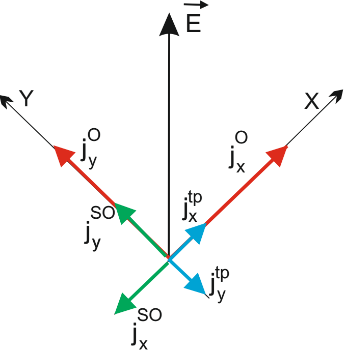
Figure 5: (a) Sketch of currents in Dirac materials: $j_{x(y)}^{O}$ is a massless ohmic current along axis $X(Y)$, $j_{x(y)}^{tp}$ is a sum of the polarization and dynamical-mass corrections to $j_{x(y)}^{O}$, $j_{x(y)}^{SO}$ is a spin-orbit contribution to $j_{x(y)}^{O}$. $\vec{E}$ is an applied electric field. (b) Frequency dependence of dielectric permeability $\Im m\ \sigma_{xx}^{tp}(-\Im m\ \sigma_{yy}^{tp})$ (magenta curve) and its fitting (blue curve) in rel.units $e^{2}/\hbar$ for the SM-model (III.19). Spectrum consists of three Majorana resonances (binding energies) $E_{1g},\ E_{2g},\ E_{3g}$ of negative (positive) charged exciton and from three anti-resonances $\overline{E}_{1g},\ \overline{E}_{2g},\ \overline{E}_{3g}$ of positive (negative) charged exciton at temperature T=3K, the higher chemical potential $\mu=135$ K. Inset shows a dimer configuration with corresponding binding (gap) energies.

At higher values of chemical potential $\mu$, contrary to the massless Dirac fermion model of graphene conductivity with one region of negative values of $\sigma_{ii}^{O}$ for a doped SM, in our non-abelian SM-model with pseudo-Majorana excitations there exist two regions with negative values of dielectric permeability $\sigma_{ii}^{O}$ in fig. 6a. One of these regions is stipulated by high value of chemical potential $\mu$ due to doping, the second one is the region of plasma oscillations owing to the presence of Majorana modes. Value of the optical conductivity $\sigma^{opt}={e^{2}\over 4\hbar}$ for SM-model with Majorana model and the massless Dirac fermion model coincide in the visible optical range and are equal to $\sigma^{opt}={e^{2}\over 4\hbar}$ in fig. 6a.

Since the precession of p_z-orbitals holds in fig. 3e, the total Ohmic massless current $\vec{J}=\vec{j}_{x}^{O}+\vec{j}_{y}^{O}$ precesses leading to emergence of a magnetic field $\vec{B}_{j}$ of non-equilibrium spin $\vec{S}$ in fig. 6b in the absence of disordered influence of substrates on $\vec{S}$. As a result of the non-equilibrium spin Hall effect (NSHE), the currents $J_{2(1)}^{spin-orbit}\sim B_{j}^{1(2)}\sigma^{spin-orbit}_{12(21)}$, $\vec{B}_{j}^{1(2)}\equiv\vec{B}_{j}^{x(y)}$ arise in the absence of an external magnetic field $\vec{B}$. At the same time, a sum $\vec{J}_{1}^{spin-orbit}+\vec{J}_{2}^{spin-orbit}$ is directed along an external magnetic field $\vec{B}_{\perp}$, which is orthogonal to the electric field applied to a sample $\vec{E}$, as it is shown in fig. 6b, and, hence, the non-equilibrium spin $\vec{S}$ is not revealed in the ordinary Hall effect. The total current $\vec{j}^{skew}=\sum_{i=1}^{2}\left(\vec{j}^{O}_{i}+\vec{J}_{i}^{spin-orbit}\right)$ is skewed, since it flows at an angle $\alpha$ to $\vec{E}$ in fig. 6b.

Thus, our model qualitatively explains experimentally observed skew topological currents in TIs Hsieh2009Science and aligned graphene/hBN superlattices Science346-2014Gorbachev at zero magnetic field.

(a)                                                                      (b)

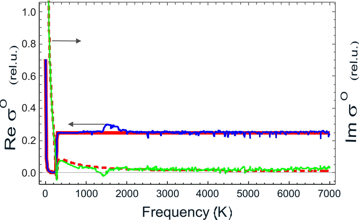
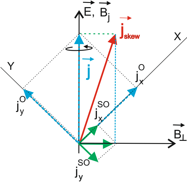
Figure 6: (a) Frequency dependencies of real (red and blue solid lines) and imaginary (dashed red and solid green lines) parts of massless ohmic contribution $\sigma_{xx(yy)}^{O}$ to the conductivity in rel.units $e^{2}/\hbar$ at very small wave number $q=10^{-8}|\vec{K}_{A}|$ for the Dirac massless fermion model Falkovsky ; Falkovsky2008PhysUspekhi (red solid and dashed lines) and for our model (III.19) (blue and green lines) , at temperature T=3K, chemical potential $\mu=135$ K. (b) Sketch of rotation of the massless ohmic SM-currents $j_{x}^{O},\ j_{y}^{O}$ (dashed lines) as a result of addition with currents $j_{2(1)}^{spin-orbit}$, generated by a magnetic field ${\vec{B}}_{j}$ of non-equilibrium spin $\vec{S}$; $\vec{j}$ is a total massless ohmic current; $\vec{j}^{skew}$ is a skew topological current. $j_{2(1)}^{spin-orbit}$ are depicted as $j_{x(y)}^{SO}$, $\vec{E}$ is an applied electric field.

V.2 Negative differential conductivity

Let graphene be disposed commensurately on the substrate, for example, of hexagonal boron nitride (graphene/hBN/graphene) or graphite so that their hexagonal lattices practically coincide (are rotated in respect to each other on a very small misalignment angle $\alpha_{m}<2^{\circ}$) Zhi-Guo-Chen-ZhiwenShi ; Pletikosic ; Woods . In this case, the resonant influence of the substrate on graphene leads to appearance of the interference long period Moiré pattern on STM- and AFM-images in fig. 7a Andrei_Rep.Prog.Phys(2012) ; G_Li .  The heterostructures at $\alpha_{m}=0$ are superlattices with center of inversion when Dirac electron and hole cone of band structures are degenerated. Accordingly, coincidence of Van Hove singularities of electron and hole densities in hyperbolic Dirac points leads to annihilation of electron-hole pairs, so that a tunnel current is vanishing at small bias $U$. The last is observed as extrema of conductance $dI/dU$ in fig. 7a Andrei_Rep.Prog.Phys(2012) ; G_Li . $U$ is the electric potential difference of the field directed transversally to the surface of the heterostructure. The polarization pair-production contribution $\sigma_{ii}^{Zitterbew}U$ and the ohmic massless current $\sigma^{O}_{ii}U$ define electron-hole contribution $I_{e-h}=(\sigma^{O}_{ii}+\sigma_{ii}^{Zitterbew})U$ into the tunnel current $I_{e-h}$ through the alignment graphene/hBN/graphene heterostructure that can be negligibly small ($I_{e-h}=0$) at small bias voltages $U$ due to recovering mirror symmetry. Since the massless Ohmic and the polarization contributions are absent, the displacement current $J$ through the heterostructure is determined by the expression $J=\Re e\ \sigma_{ii}^{add}(U)U$ only. The bias current $J$ increases the heterostructure energy on a value $\hbar\omega=CU^{2}/2+A_{0}$, where $C$ is the electric capacitance of the heterostructure and $A_{0}$ is a constant. Then the dependence $J=\Re e\ \sigma_{ii}^{add}(\omega)U$ in fig. 7b can be found with the condition $U\sim\sqrt{\hbar\omega}$. The current increase in volt-ampere characteristics in fig. 7b is followed to its decrease in some range of values of $U$ that is known as a phenomenon of negative differential conductivity. Our theoretically predicted dependence $J$ on $U$ is completely consistent with the experimental data represented in Twist-controlled-resonant-tunnelling-in-graphene-boron-nitride-graphene2014 , as fig. 7b demonstrates.

(a)                                                                      (b)

Figure 7: (a) Conductance $dI/dU$ as a function of voltage $U$ applied to twisted graphene placed on graphite for a sample with large Moiré pattern (inset, scale 2 nm) at $1.16^{\circ}$ misalignment angle G_Li . (b) Dependence of tunnel current $J$ on the bias voltage $U$ for heterostructure graphene/hBN/graphene: an experimental curve at $1.8^{\circ}$ misalignment angle (black solid curve), a theoretical one (green dashed curve) from Twist-controlled-resonant-tunnelling-in-graphene-boron-nitride-graphene2014 , our theoretical simulation (red solid curve) of $J$ in the SM-model (III.19) at temperature T=3K, chemical potential $\mu=135$ K with its fitting (blue solid curve).

V.3 Longitudinal conductivity

For attacking the so called ”minimal dc-conductivity” problem Ando2002 ; Ziegler it is important to obtain the frequency dependence of longitudinal dc-conductivity for frequencies $\omega\to 0$ and non-vanishing wave vectors $\vec{k}=\vec{p}/\hbar-\vec{K}_{A(B)}$. The longitudinal conductivity $\sigma_{L}(\omega,{\vec{k}})$ is defined through the conductivity tensor splitting into longitudinal and transversal terms as Kraft-Ropke

$$\sigma_{ij}(\omega,{\vec{k}})=\left(\delta_{ij}-\frac{k_{i}k_{j}}{{\vec{k}}^{2}}\right)\sigma_{T}(\omega,{\vec{k}})+\frac{k_{i}k_{j}}{{\vec{k}}^{2}}\sigma_{L}(\omega,{\vec{k}}).$$ (V.5)

Let us consider an influence of spatial dispersion on longitudinal conductivity at low frequencies $\omega=10^{-10}$, $4\times 10^{-3}$, 13.3 K for graphene models $N=2,\ 3$ in fig. 1. According to the numerical results in fig. 8, the dielectric permeability (imaginary part of complex conductivity $\Im m\ \sigma^{O}_{ii}$ ) of non-doped graphene in the massless Dirac fermion model $N=2$ with spatial dispersion is positive at $\omega=4\times 10^{-3}$ and 13.3 K, but takes zero value at $\omega=10^{-10}$ K. In the model $N=3$ with spatial dispersion, the dielectric permeability can gain zero and negative values at all these frequencies. Regions with zero and negative values of the dielectric permeability are regions of plasmonic oscillations where the complex frequencies $\omega(k_{pl})+i\gamma(k_{pl})$ satisfy the following equation Platzmann-Wolf1973 ; Mikhaylovski1977 :

$$\Im m\ \sigma_{ii}^{O}(k,z)-i\Re e\ \sigma_{ii}^{O}(k,z)=0,\ z=\omega+i\gamma.$$ (V.6)

Expanding eq. (V.6) into series in terms of powers of $i\gamma$ in the vicinity of plasmonic resonance $\omega_{pl}$, $\Im m\ \sigma_{ii}^{O}(k_{pl},\omega(k_{pl}))=0$ gives the dumping constant for the plasmons

$$\gamma(k_{pl})=\left.{\Re e\ \sigma_{ii}^{O}(\omega(k))\over\frac{\partial\Im m\ \sigma_{ii}^{O}(\omega(k))}{\partial k}\left(\frac{\partial\omega(k)}{\partial k}\right)^{-1}}\right|_{k=k_{pl}}.$$ (V.7)

According to simulation presented in fig. 8a, $\Im m\ \sigma_{ii}^{O}(k,\omega)$ at $\omega=10^{-10}$ K is practically constant function in the model $N=2$, and, hence, the expression (V.7) diverges. Therefore, contrary to the model $N=3$, the plasmon damping occurs instantly in the model $N=2$, $\gamma^{N=2}\to\infty$. Long living plasmons in the SM-model $N=3$ are able to provide screening in the electrophysical range. The massless Dirac fermion model with instantly damped plasmon oscillations does not allow to describe screening of an external electric field.

(a)                                                                       (b)
     

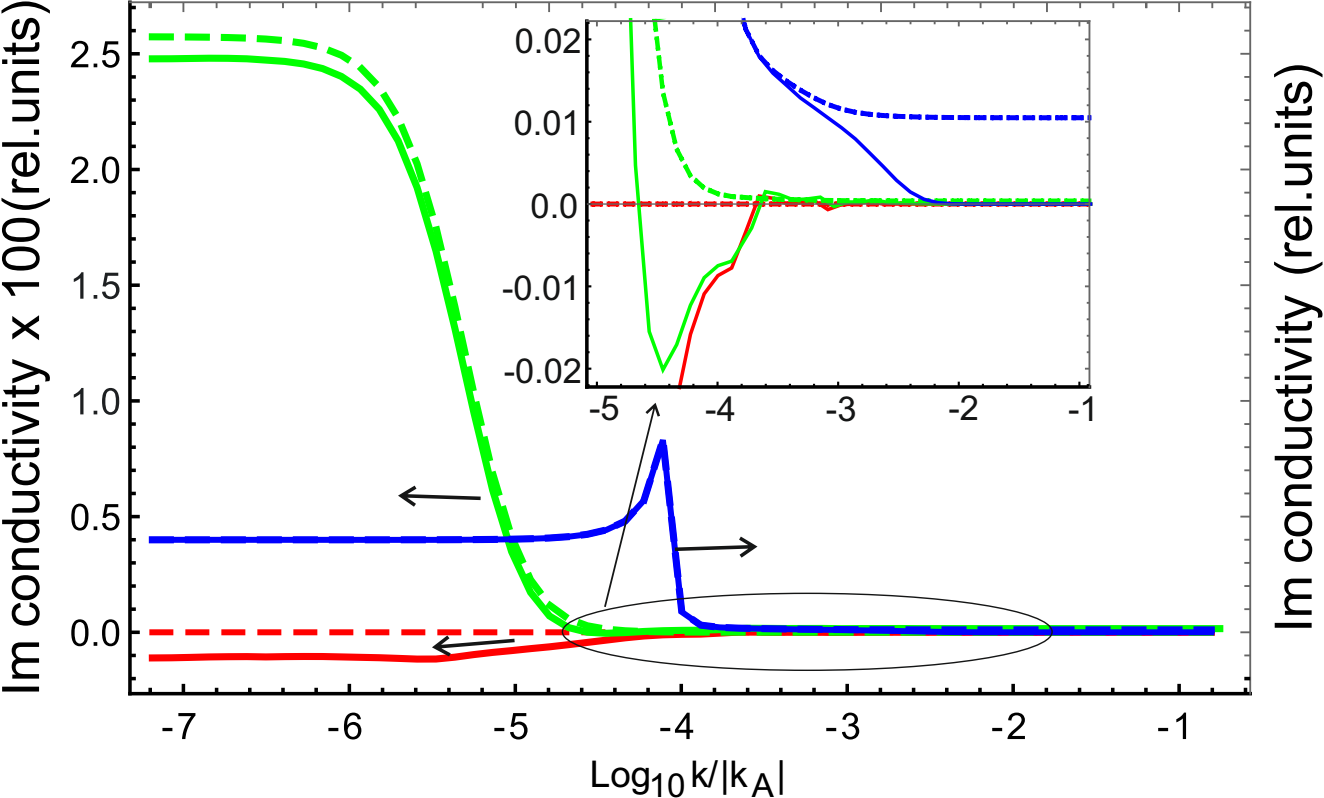
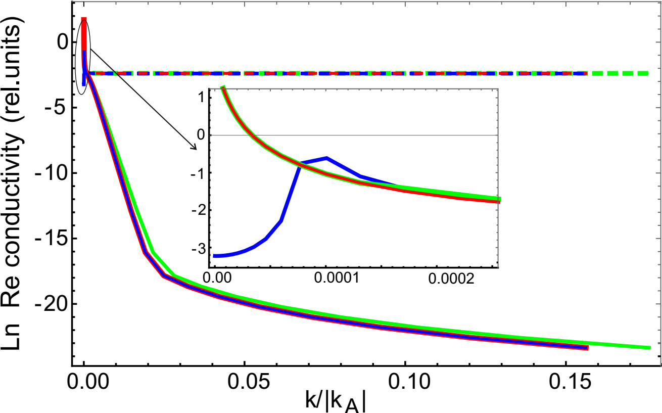
Figure 8: Imaginary (a) and real (b) parts of longitudinal massless ohmic contribution $\sigma_{xx(yy)}^{O}$ to conductivity vs wave number $k$, $\vec{k}=\vec{p}-\vec{K}_{A(B)}$ for our SM-model $N=3$ (III.19) (solid curves) and for the massless Dirac fermion model Falkovsky (dashed curves), at temperature 100 K and frequencies 13.3 K ($0.27$ THz, blue color), $4\times 10^{-3}$ K ($83$ MHz, green color), $10^{-10}$ K ($2.08$ Hz, red color); chemical potential equals to 1 K. Inset to figure (a) demonstrates the behaviour of $\Im m\ \sigma_{xx(yy)}^{O}$ in a neighborhood of small values; inset to figure (b) demonstrates the behaviour of $\Re e\ \sigma_{xx(yy)}^{O}$ in the region of small $k$ .

Let us calculate the dc-conductivity $\sigma^{dc}$. We perform the inverse Fourier transformation as

$$\sigma^{dc}={1\over(2\pi)^{2}}\int{\sigma^{O}_{\|}}(\omega,k)e^{i\vec{k}\cdot\vec{r}}d^{2}k.$$ (V.8)

According to fig. 8b, the Fourier image ${\sigma^{O}_{\|}}(\omega,k)$ of longitudinal conductivity at $\omega=10^{-10}$ K for the graphene model $N=3$ behaves itself approximately as the Dirac $\delta$-function, that is equal zero everywhere except of $k\to 0$, where $\sigma^{O}_{\|}(\omega,0)=5.49e^{2}/\hbar$. Hence, the dc-conductivity (V.8) in the model $N=3$ gains non-zero value

$$\sigma^{dc,N=3}(\omega)={1\over(2\pi)^{2}}\int\sigma^{O}_{\|,N=3}(\omega,k)e^{i\vec{k}\cdot\vec{r}}d^{2}k\approx{1\over 2\pi}\int\sigma^{O}_{\|N=3}(\omega,0)\delta(|k|)e^{i\vec{k}\cdot\vec{r}}dk={5.49e^{2}\over h},\ \omega=10^{-10}~{}K$$ (V.9)

at temperature 100 K and chemical potential 1 K. Contrary to this, the Fourier image of the dc-conductivity in the graphene model $N=2$ takes a constant value at large wave numbers $k$, hence, integrand in inverse Fourier transformation of $\sigma^{dc,N=2}(\omega)$ in (V.8) is a highly oscillating function leading to zero value of the minimal dc-conductivity $\sigma^{dc,N=2}(\omega)$, $\sigma^{dc,N=2}(\omega)=0$.

The minimal dc-conductivity of graphene in devices with large area of graphene monolayer on SiO₂ turns out to be $\sigma_{min}\sim 4e^{2}/h$ Novoselov2004 at low temperatures ($\sim 1.5$ K). The minimal dc-conductivity of suspended graphene Bolotin ; Du and of graphene on boron nitride substrate Dean is $\sigma_{min}\sim 6e^{2}/h$ at $T\sim 300$ K. Thus, our estimate (V.9) is in a perfect agreement with experimental data.

V.4 Chiral anomaly, longitudinal magneto-conductivity, and splitting zero-bias conductance peaks

As it is sketched in fig. 3e,  p_z-orbitals precess. Accordingly, the topological currents $j^{tp}_{x(y)}\propto\sigma_{xx(yy))}^{tp}$ precess as well, creating magnetic fields $\vec{B}_{x(y)}^{tp}$ in fig. 9a. Let us denote the resulting magnetic field $\vec{B}_{x}^{tp}+\vec{B}_{y}^{tp}$ through $\vec{\Omega}_{M}$.

Generally, external electromagnetic fields $\left\{\vec{A},\Phi\right\}$ reorient randomly the directions of magnetic fields $B^{tp}_{x(y)}$, disordering the vortex SM-lattice and, as a result, breaking topological currents $j^{tp}_{x(y)}\propto\sigma_{xx(yy))}^{tp}$. Let us place SM on superconducting substrate S. Then, nearly located and having equal topological charges vortexes of SM and S repel each other. As a result, the vortex regions characterized by the definite sign $\pm$ of topological charge appear in SM. If vortex lattices of SM and S are consistent, topological components $j^{tp}_{x(y)}$ of the current linked with $\vec{B}_{x(y)}^{tp}$ are rotated in an external magnetic field $\vec{B}_{\|}$ at conditions that $\vec{B}_{\|}\perp\vec{\Omega}_{M}$ and the electric field $\vec{E}$ and $\vec{B}_{\|}$ are parallel: $\vec{E}\|\vec{B}_{\|}$. Let us denote the distribution of the magnetic fields inside a sample through $\left.\{\vec{B}_{i,SM}\}\right|_{i=1}^{N}$, $N$ is a number of hexagons. $\vec{\Omega}_{M}$ is aligned along the direction of the effective magnetic field $\vec{B}_{eff}=\vec{B}_{\|}+\sum_{i=1}^{N}\vec{B}_{i,SM}=\vec{B}_{\|}+\vec{B}_{SM}$ and hence, is directed at an angle $\alpha$ to the electric field $\vec{E}$. Meanwhile, the topological current $\vec{J}_{ZBP}$ (ZBP), called as a zero-bias peak, emerges in the direction $\vec{E}$ as

$$J_{ZBP}\propto\Omega_{M}\cos\alpha.$$ (V.10)

Scheme of this phenomenon is demonstrated in fig. 9a.

If the magnetic field $\sum_{i=1}^{N}\vec{B}_{i,SM}$ is small compared with the magnitude of the applied field $\vec{B}_{\|}$: $\vec{B}_{SM}\ll\vec{B}_{\|}$, then $\vec{\Omega}_{M}=\vec{\Omega}_{1,M}N$ trends to align along $\vec{B}_{\|}$ in the absence of the electric $\vec{E}$. Accordingly, the value $J_{ZBP}$ trends to the quantum limit $\sum_{i=1}^{N}(\vec{j}^{tp}_{i,x}+\vec{j}^{tp}_{i,y})$. The quantity $\left|\vec{j}^{tp}_{1,x}+\vec{j}^{tp}_{1,y}\right|$ is proportional to the Majorana conductivity Goudarzi2017PhysicaE ; Peng-Falko2015PRL .

Now, let us consider the case $\sum_{i=1}^{N}\vec{B}_{i,SM}\gg\vec{B}_{\|}$. Then the following approximation for $\vec{\Omega}_{M}$ holds

$$\vec{\Omega}_{M}\approx\vec{\Omega}_{1,M}n_{1}+\Omega_{1,M}n_{2}\vec{B}_{SM}/|B_{SM}|,\ \ n_{1}\propto B_{\|},\ n_{1}+n_{2}=N.$$ (V.11)

Here $\vec{\Omega}_{1,M}=\sum_{i=1}^{2}\vec{B}^{tp}_{1,i}$, $B^{tp}_{1,x(y)}$ are magnetic fields, generated by the topological currents $j^{tp}_{1,x(y)}$ in one hexagon. Then, the current $\vec{J}_{ZBP}$ (V.10) is approximated by the following expression:

$$J_{ZBP}\propto\Omega_{1,M}(\cos\alpha)B_{\|}.$$ (V.12)

Contrary to the ordinary Hall effect, the contributions $\sigma_{xx}^{tp}$ and $\sigma_{yy}^{tp}$ reveal themselves in the magnetic field $\vec{B}_{\|}$, directed along the electric field $\vec{E}$, when the current orthogonal to $\vec{E}$, $\vec{j}^{tp}_{x}+\vec{j}^{tp}_{y}$, $j^{tp}_{i}\propto\sigma_{ii}^{tp}$ is rotated in the field $\vec{B}_{\|}$ due to alignment of the spin of precessing $\pi($p${}_{z})$-orbital at the angle $\alpha$ to $\vec{B}_{\|}$, as it is shown in fig. 9a. Hence, the longitudinal magneto-conductivity is observed. Berry curvature $\vec{\Omega}_{k}$ leads to the change of the velocity of the charged particle from $\vec{v}$ in the field $\vec{E}$ to $\vec{\dot{r}}$ in the field $\vec{B}_{\|}$ and $\vec{E}$, $\vec{E}\,\|\,\vec{B}_{\|}$ as Lu-Shen2017Front-Phys ; Yip2015Preprint

$$\vec{\dot{r}}=\vec{v}+{e\over\hbar}\left(\vec{\Omega}_{k}\cdot\vec{v}\right)\vec{B}_{\|},\ \vec{v}\|\vec{E}.$$ (V.13)

Right hand sides of (V.12) and (V.13) are similar, but $\vec{\Omega}_{M}$ is a curvature of our Majorana model system. Eq. (V.12) describes negative magnetoresistance (NMR) that represents the phenomenon of chiral anomaly at weak magnetic fields parallel to electric ones H-ZhLuSh-QShen2017 ; Niemann2017 .

Bounding the vortex lattice of SM to the vortex lattice of the S-substrate NMR manifests itself as a splitting zero-bias conductance peak (SZBP) in fig. 9b at higher values of chemical potential. The real part of the frequency dependence of $\sigma_{xx(yy)}^{tp}$ for higher chemical potential is calculated based on the formula (V.3) and is represented in fig. 9c. The two low-frequency peaks similar to SZBP with the height of about $\sim 0.24\sigma^{opt}\sim 0.3768e^{2}/h$ are observed in fig. 9c. For one-dimensional SM possessing strong SOC, the height of ZBP would be four times smaller $\sim 0.0942e^{2}/h$. The last coincides with experimentally measured in Das2012Nat-Phys ZBP ($\approx 0.1e^{2}/h$) for such 1D topological superconductor as an indium arsenide nanowire on an aluminium superconductor substrate. The effective magnetic field $\vec{B}_{eff}$ in a sample is determined through the competition between vortex-vortex repulsion and Lorentz force in an external magnetic field. Therefore, SZBP disappears in strong external magnetic fields $\vec{B}$, as it is shown in fig. 9b.

(a)                                                             (b)                                                              (c)

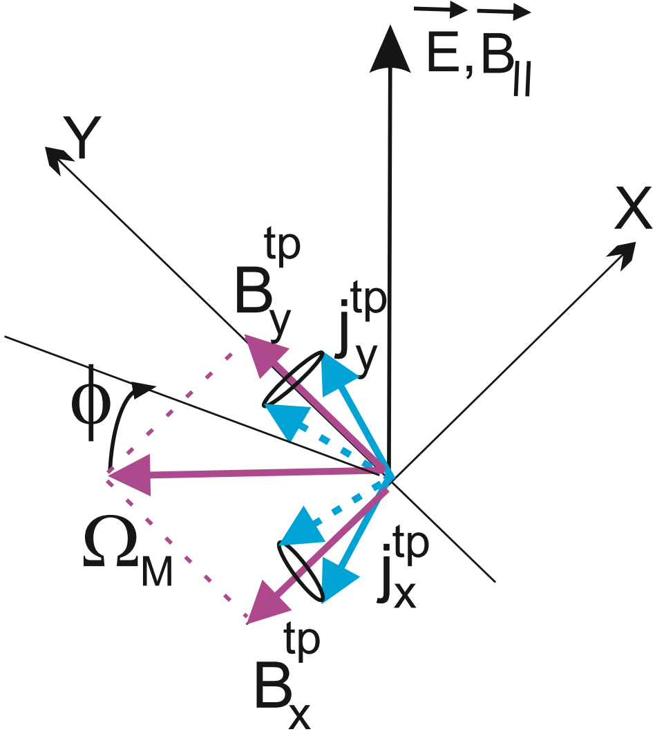
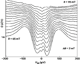
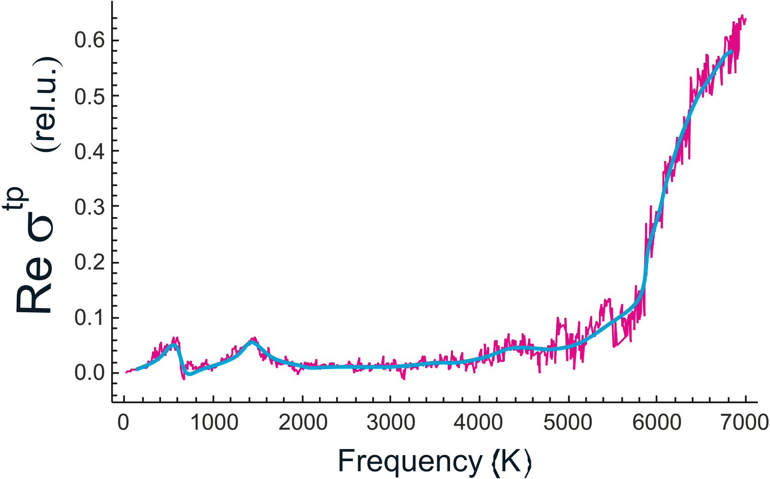
Figure 9: (a) Sketch of splitting zero-bias conductance peak: ${\vec{B}}^{tp}_{x(y)}$ is a magnetic field of precessing spins of $\pi$(p_z)-orbitals, $\phi$ is a turn angle of the Majorana curvature $\vec{\Omega}_{M}$ in a magnetic field $\vec{B}_{\|}$, parallel to electric field $\vec{E}$. (b) Experimental low-bias conductance as a function of applied magnetic field parallel to axis of an induced one-dimensional topological superconductor (a system composed of an aluminium superconductor in proximity to an indium arsenide nanowire) at a higher chemical potential, from Das2012Nat-Phys . (c) Our theoretical simulation of SZBP by the semimetal-model Hamiltonian (III.19) as two low-frequency peaks in the frequency dependence of real part of topological conductivity $\sigma_{xx}^{tp}$ (magenta solid curve) and its fitting (blue solid curve) in rel.units $e^{2}/\hbar$ at temperature T=3K and chemical potential $\mu=135$ K.

Magnetic-field-induced ZBP and its splitting, as expected for zero-energy Majorana state, were observed in Mourik2012Science ; Deng2012Preprint . Magnetic pinning of vortices in S/1D-ferromagnetic heterostructures DiGiorgio2016ScientificReports Oppen-Peng-Pientka-Oxford2017 , hybrid S/ferromagnetic TI Koren2011PhysRevB , and graphene/S Dirks2011NaturePhysics structures is called a proximity effect Buzdin2005RevModPhys ; LiangFu-Kane2008PRL . Formation of superconductor-vortex clusters on topological defects in 1D-ferromagnetic materials is possible DiGiorgio2016ScientificReports . Magnetic anisotropy of all these heterostructures manifests itself in an external magnetic field in the form of quantized zero-bias conductance peak Goudarzi2017PhysicaE ; Peng-Falko2015PRL ; Das2012Nat-Phys ; Yang2011 .

VI Discussion and Conclusion

Finalizing our finding, a ${\mathbb{Z}}_{2}$ topological semimetal model with a number of internal degrees of freedom (flavors) $N=3$ has been proposed, with three-body excitations as charge carriers. A novel Majorana-like quantum-field approach allows to calculate low-frequency conductivity with accounting of the polarization and magnetoelectric effects. Using this approach, braiding Majorana particles have been found and interpreted as dimer configurations in the RVB-picture. The developed non-abelian quantum statistics predicts three flavor pairs Majorana resonance–antiresonance.

Dichroism of Dirac bands for the ${\mathbb{Z}}_{2}$ SM-model is provided by the vortex structure of the Dirac bands due to existence of zero-energy Majorana modes and chiral braiding Majorana modes. It has been shown that the deconfinement of the Majorana-like modes leads to the appearance of a set of gapless Fermi arcs.

Chiral-anomaly revealed in charge transport in the form of zero-bias conductance peak and its splitting is a specific feature of the SM-model $N=3$ with skew topological currents in zero magnetic fields. This splitting peak is stipulated by non-zero curvature of the Majorana model.

In the model $N=3$ there exists a mechanism for dynamical reduction of spatial dispersion of states. This dynamic reduction provides a non-zero value of minimal dc-conductivity of graphene. Plasmonic oscillations in the massless Dirac fermion model occur in electrophysic frequency range $\omega\lesssim 2$ Hz, but practically dump instantly. Contrary to this, the plasmonic oscillations in the Majorana-like massless fermion model have a finite dumping rate and exist both in optical and electrophysic frequency ranges.

Significant advantage of the proposed Majorana-like fermion theory augment by a mixing mass term over the massless Dirac fermion and Weyl SM-models consists in the achieved qualitative and quantitative consistency with experimentally observable properties of topological semimetals. The ${\mathbb{Z}}_{2}$ topological SM-model with the flavors number $N=3$ can be considered as an effective tools to discover and investigate new Dirac materials and to develop new devices for quantum computing.

Acknowledgments. This work has been supported in part by the State Scientific Program of Fundamental Researches ”Convergence-2020” of Belarus.

Supplementary Information

I Band-structure simulation details

Bispinor wave functions of quasiparticles can be represented through free Dirac fields of $\pi$ (p_z)-electrons:

$$\left(\begin{array}[]{c}\widehat{\chi^{\dagger}_{-\sigma_{{}_{A(B)}}}}(\vec{r})\left|0,-\sigma\right>\\ \widehat{\chi^{\dagger}_{\sigma_{{}_{B(A)}}}}(\vec{r})\left|0,\sigma\right>\end{array}\right)={e^{-\imath(\vec{K}_{A(B)}-\vec{q}_{{}_{A(B)}})\cdot\vec{r}}\over\sqrt{2}}\left(\begin{array}[]{c}\exp\{-\imath\theta_{k_{A(B)}}\}\phi_{1}\\ \exp\{-\imath\theta_{k_{A(B)}}\}\phi_{2}\\ -\exp\{\imath\theta_{k_{B(A)}}\}\phi_{2}\\ \exp\{\imath\theta_{k_{B(A)}}\}\phi_{1}\end{array}\right)\equiv\left(\begin{array}[]{c}\chi_{-\sigma_{A(B)}}\\ \chi_{+\sigma_{B(A)}}\end{array}\right),\ \$$ (S.9)

$$\left(\begin{array}[]{c}\widehat{\chi^{\dagger}_{+\sigma_{{}_{A(B)}}}}(\vec{r})\left|0,\sigma\right>\\ \widehat{\chi^{\dagger}_{-\sigma_{{}_{B(A)}}}}(\vec{r})\left|0,-\sigma\right>\end{array}\right)={e^{-\imath(\vec{K}_{A(B)}-\vec{q}_{{}_{A(B)}})\cdot\vec{r}}\over\sqrt{2}}\left(\begin{array}[]{c}-\exp\{\imath\theta_{k_{A(B)}}\}\phi_{2}\\ \exp\{\imath\theta_{k_{A(B)}}\}\phi_{1}\\ \exp\{-\imath\theta_{k_{B(A)}}\}\phi_{1}\\ \exp\{-\imath\theta_{k_{B(A)}}\}\phi_{2}\end{array}\right)\equiv\left(\begin{array}[]{c}\chi_{+\sigma_{A(B)}}\\ \chi_{-\sigma_{B(A)}}\end{array}\right)$$ (S.18)

where $\theta_{k_{B(A)}}$ are phases for free fermion fields Peskin-Schroeder ,

$$\phi_{i}={1\over(2\pi)^{3/2}\sqrt{N/2}}\sum_{\vec{R}^{A(B)}_{l}}\exp\{\imath[\vec{K}_{A(B)}-\vec{q}_{{}_{A(B)}}][\vec{R}^{A(B)}_{l}-\vec{r}]\}\psi_{\{n_{i}\}}(\vec{r}-\vec{R}^{A(B)}_{l})\ \ \ \ \ \ \ \$$ (S.19)

is a Bloch function; maximally-localized Wannier functions $\psi_{\{n_{i}\}}$, $i=1,2$ are defined as

$$\psi_{\{n_{2}\}}=c_{1}\psi_{\mbox{\small p}_{z}}(\vec{r}\pm\vec{\delta}_{i})+c_{2}\psi_{\mbox{\small p}_{z}}(\vec{r}),\ \sum_{i=1}^{2}c_{i}^{2}=1;\\ \psi_{\{n_{1}\}}=\psi_{\mbox{\small p}_{z}}(\vec{r});$$ (S.20)

$\vec{\delta}_{i}$ is a distance to nearest $i-$th site $\vec{\delta}_{i}$, $i=1,2,3$; definition of wave vector $\vec{q}_{{}_{A(B)}}$ uses the reference frame origin located in the Dirac point $K_{A(B)}$, $\psi_{\mbox{\small p}_{z}}(\vec{r})$ is the p_z-wave function of a hydrogen-like atom with an ”effective charge”  1 centered at the graphene lattice sites.

An exchange interaction term $\left(\Sigma_{rel}^{x}\right)_{AB}$ is determined as myNPCS2013 ; myNPCS17-2014 ; NPCS18-2015GrushevskayaKrylovGaisyonokSerow

$$\Sigma_{rel}^{x}\left(\begin{array}[]{c}\widehat{\chi}^{\dagger}_{{}_{-\sigma_{{}_{A}}}}(\vec{r})\\ \widehat{\chi}^{\dagger}_{\sigma_{{}_{B}}}(\vec{r})\end{array}\right)\left|0,-\sigma\right>\left|0,\sigma\right>=\left(\begin{array}[]{cc}0&\left(\Sigma_{rel}^{x}\right)_{AB}\\ \left(\Sigma_{rel}^{x}\right)_{BA}&0\end{array}\right)\left(\begin{array}[]{c}\widehat{\chi}^{\dagger}_{-\sigma_{{}_{A}}}(\vec{r})\\ \widehat{\chi}^{\dagger}_{\sigma_{{}_{B}}}(\vec{r})\end{array}\right)\left|0,-\sigma\right>\left|0,\sigma\right>,$$ (S.27)

$$\left(\Sigma_{rel}^{x}\right)_{AB}\widehat{\chi}^{\dagger}_{\sigma_{{}_{B}}}(\vec{r})\left|0,\sigma\right>=\sum_{i=1}^{N_{v}\,N}\int{d\vec{r}_{i}}\widehat{\chi}^{\dagger}_{\sigma_{i}{{}^{B}}}(\vec{r})\left|0,\sigma\right>\langle 0,-\sigma_{i}|{\widehat{\chi}}^{\dagger}_{-\sigma_{i}^{A}}(\vec{r}_{i})V(\vec{r}_{i}-\vec{r}){\widehat{\chi}}_{-\sigma_{B}}(\vec{r}_{i})|0,-\sigma_{i^{\prime}}\rangle,$$ (S.28)

$$\left(\Sigma_{rel}^{x}\right)_{BA}\widehat{\chi}^{\dagger}_{{}_{-\sigma_{{}_{A}}}}(\vec{r})\left|0,-\sigma\right>=\sum_{i^{\prime}=1}^{N_{v}\,N}\int{d\vec{r}_{i^{\prime}}}\widehat{\chi}^{\dagger}_{{}_{-\sigma_{i^{\prime}}^{A}}}(\vec{r})\left|0,-\sigma\right>\langle 0,\sigma_{i^{\prime}}|{\widehat{\chi}}^{\dagger}_{\sigma_{i^{\prime}}^{B}}(\vec{r}_{i^{\prime}})V(\vec{r}_{i^{\prime}}-\vec{r}){\widehat{\chi}}_{{}_{\sigma_{A}}}(\vec{r}_{i^{\prime}})|0,\sigma_{i}\rangle.$$ (S.29)

In the approximation of free $\pi$-electrons, all wave functions entering the expression (S.28, S.29) are

$$\begin{split}\widehat{\chi}^{\dagger}_{-\sigma_{i^{\prime}}{{}^{A}}}(\vec{r})\equiv\widehat{\chi^{\dagger}_{-\sigma_{{}_{A}}}}(\vec{r}),\ \ \widehat{\chi}^{\dagger}_{\sigma_{i}{{}^{B}}}(\vec{r})\equiv\widehat{\chi^{\dagger}_{\sigma_{{}_{B}}}}(\vec{r})\mbox{ for }\forall\ i,\ i^{\prime}.\end{split}$$ (S.30)

Then, in this approximation we can write matrices $\left(\Sigma_{rel}^{x}\right)_{AB}\approx\Sigma_{AB}$ and $\left(\Sigma_{rel}^{x}\right)_{BA}\approx\Sigma_{BA}$ without self-action as

$$\left(\Sigma_{rel}^{x}\right)_{AB}\widehat{\chi^{\dagger}_{+\sigma_{{}_{B}}}}(\vec{r})\left|0,\sigma\right>\approx\Sigma_{AB}\ \chi_{\sigma_{B}}=\sum_{i=1}^{N_{v}N-1}\int d\vec{r}_{i}$$

$$\times V(\vec{r}_{i}-\vec{r})\left[\chi_{-\sigma_{A}}(\vec{r}_{i})\cdot\chi_{-\sigma_{B}}^{*}(\vec{r}_{i})\right]\chi_{+\sigma_{B}}(\vec{r})={1\over 2^{3/2}}\sum_{i=1}^{N_{v}N-1}\int d\vec{r}_{i}V(\vec{r}_{i}-\vec{r})$$

$$\times\left[\begin{array}[]{cc}e^{-\imath\theta_{K_{A}}}\phi_{1}(\vec{r}_{i})e^{\imath\theta_{K_{B}}}\phi^{*}_{1}(\vec{r}_{i})&e^{-\imath\theta_{K_{A}}}\phi_{1}(\vec{r}_{i})e^{\imath\theta_{K_{B}}}\phi^{*}_{2}(\vec{r}_{i})\\ e^{-\imath\theta_{K_{A}}}\phi_{2}(\vec{r}_{i})e^{\imath\theta_{K_{B}}}\phi^{*}_{1}(\vec{r}_{i})&e^{-\imath\theta_{K_{A}}}\phi_{2}(\vec{r}_{i})e^{\imath\theta_{K_{B}}}\phi^{*}_{2}(\vec{r}_{i})\end{array}\right]\left[\begin{array}[]{c}-e^{-\imath[(\vec{K}_{A}-\vec{q}_{A})\cdot\vec{r}-\theta_{K_{B}}]}\phi_{2}(\vec{r})\\ e^{-\imath[(\vec{K}_{A}-\vec{q}_{A})\cdot\vec{r}-\theta_{K_{B}}]}\phi_{1}(\vec{r})\end{array}\right],$$ (S.35)

$$\left(\Sigma_{rel}^{x}\right)_{BA}\widehat{\chi^{\dagger}_{-\sigma_{{}_{A}}}}(\vec{r})\left|0,-\sigma\right>\approx\Sigma_{BA}\ \chi_{-\sigma_{A}}=\sum_{i=1}^{N_{v}N-1}\int d\vec{r}_{i}$$

$$\times V(\vec{r}_{i}-\vec{r})\left[\chi_{+\sigma_{B}}(\vec{r}_{i})\cdot\chi_{+\sigma_{A}}^{*}(\vec{r}_{i})\right]\chi_{-\sigma_{A}}(\vec{r})={1\over 2^{3/2}}\sum_{i=1}^{N_{v}N-1}\int d\vec{r}_{i}V(\vec{r}_{i}-\vec{r})$$

$$\times\left[\begin{array}[]{cc}-e^{\imath\theta_{K_{B}}}\phi_{2}(\vec{r}_{i})(-1)e^{-\imath\theta_{K_{A}}}\phi^{*}_{2}(\vec{r}_{i})&-e^{\imath\theta_{K_{B}}}\phi_{2}(\vec{r}_{i})e^{-\imath\theta_{K_{A}}}\phi^{*}_{1}(\vec{r}_{i})\\ e^{\imath\theta_{K_{B}}}\phi_{1}(\vec{r}_{i})(-1)e^{-\imath\theta_{K_{A}}}\phi^{*}_{2}(\vec{r}_{i})&e^{\imath\theta_{K_{B}}}\phi_{1}(\vec{r}_{i})e^{-\imath\theta_{K_{A}}}\phi^{*}_{1}(\vec{r}_{i})\end{array}\right]\left[\begin{array}[]{c}e^{-\imath[(\vec{K}_{A}-\vec{q}_{A})\cdot\vec{r}+\theta_{K_{A}}]}\phi_{1}(\vec{r})\\ e^{-\imath[(\vec{K}_{A}-\vec{q}_{A})\cdot\vec{r}+\theta_{K_{A}}]}\phi_{2}(\vec{r})\end{array}\right].$$ (S.40)

It follows from the expressions (S.35, S.40) that the matrices $\Sigma_{AB}$ and $\Sigma_{BA}$ have the form

$$\Sigma_{AB}={1\over 2}e^{\{-\imath(\theta_{K_{A}}-\theta_{K_{B}})\}}\sum_{i=1}^{N_{v}N-1}\int d\vec{r}_{i}V(\vec{r}_{i}-\vec{r})\left[\begin{array}[]{cc}\phi_{1}(\vec{r}_{i})\phi^{*}_{1}(\vec{r}_{i})&\phi_{1}(\vec{r}_{i})\phi^{*}_{2}(\vec{r}_{i})\\ \phi_{2}(\vec{r}_{i})\phi^{*}_{1}(\vec{r}_{i})&\phi_{2}(\vec{r}_{i})\phi^{*}_{2}(\vec{r}_{i})\end{array}\right],$$ (S.43)

$$\Sigma_{BA}={1\over 2}e^{\{-\imath(\theta_{K_{A}}-\theta_{K_{B}})\}}\sum_{i=1}^{N_{v}N-1}\int d\vec{r}_{i}V(\vec{r}_{i}-\vec{r})\left[\begin{array}[]{cc}\phi_{2}(\vec{r}_{i})\phi^{*}_{2}(\vec{r}_{i})&-\phi_{2}(\vec{r}_{i})\phi^{*}_{1}(\vec{r}_{i})\\ -\phi_{1}(\vec{r}_{i})\phi^{*}_{2}(\vec{r}_{i})&\phi_{1}(\vec{r}_{i})\phi^{*}_{1}(\vec{r}_{i})\end{array}\right].$$ (S.46)

The quasirelativistic Dirac–Hartree–Fock exchange interaction (S.43, S.46) in tight-binding approximation are determined by Eqs. (III.3, III.6) of the main text. In the direction perpendicular to the SM layer, the integration has been limited to a distance equals two C–C bond lengths, the phases have been chosen as $\theta_{K_{A}}=\theta_{K_{B}}$.

Simulations of the band structure have been performed for two variants of approximation to the exchange operator. The first one already mentioned above is the series expansion of the exchange matrices on deviation of the wave vector from the Dirac point up to 4th order in the length of wave vector $\vec{q}$. As it has been shown in myJModPhys2014 ; myNATO2015 ; NPCS18-2015GrushevskayaKrylovGaisyonokSerow ; myNPCS18-2015 , this approximation leads to small imaginary part for the energy (spectral line width), this in fact not very bad as it effectively corresponds to a finite decay. The approximation of the zero gauge-phases is valid in the Dirac point.

The second approximation is the use of the exchange interaction matrices calculated based on $\pi$(p_z)-orbital wave functions with full exponents and with non-zero gauge-phases (see the detail of the approximation in NPCS18-2015GrushevskayaKrylovGaisyonokSerow ; myNPCS18-2015 ; myIntJModPhys2016 ; mySymmetry2016 ). The last approximation holds real eigenenergies for all wave vectors. The condition of the real values for the energy playing a role of the gauge condition in the second approximation has been achieved by minimization (on respect to a given phases set) of its imaginary part. This results into finite accuracy at the energy evaluation in situation with non-zero phases.

Numerical simulations of eigenenergies have been performed for approximately $3500\times 200$ grid points $(r,\ \phi)$ in 2D $\vec{q}$-space for the purposes of subsequent estimation of charge transport properties of the system. For simulations we use the spectral line width equals to 1 K.

The calculated Majorana model bands $\epsilon$ in fig. 3a and fig. S.1 have the form of cones near the Dirac point $K_{A(B)}$ at wave numbers $q<0.0002K_{A}$. Then the Dirac cone is splitted, and eight tilted sub-replicas emerge at large $q$.

(a)                                                                       (b)

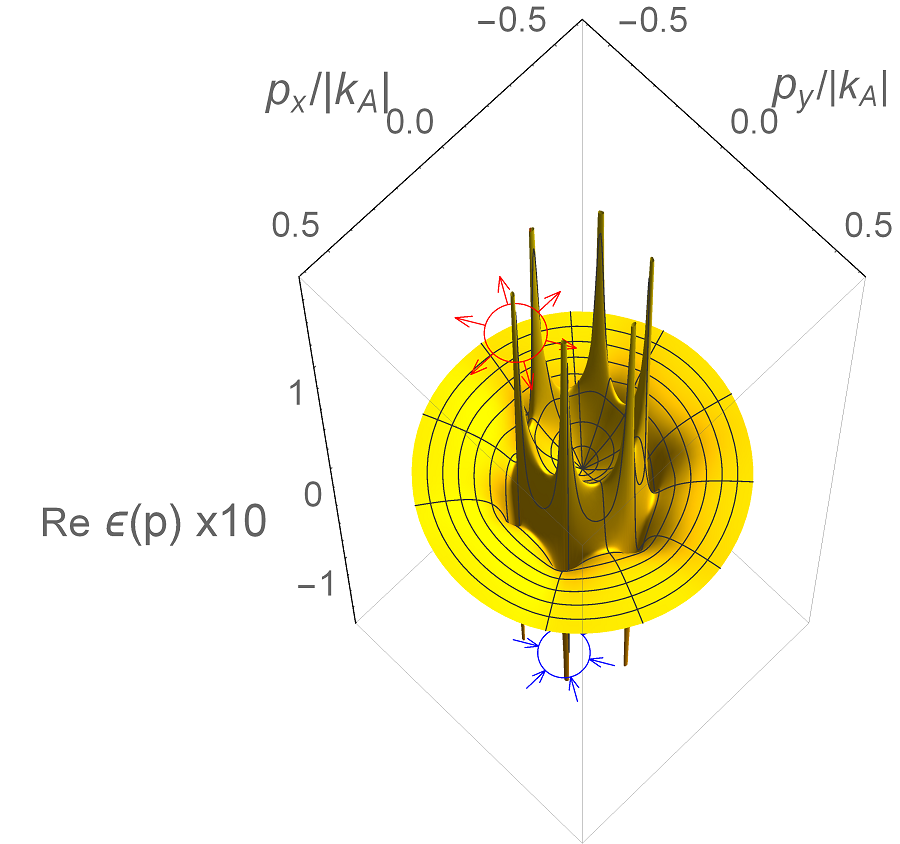
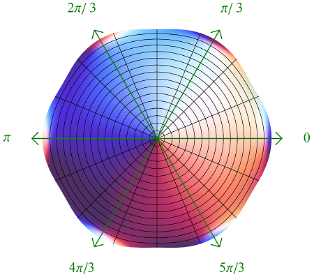
(c)

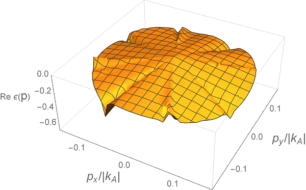
Figure S.1: Energy bands of 2D semi-metal calculated in two approximations: (a, b) in the first-order approximation with zero gauge phases in 4th order Taylor series expansion of exponential factors of the exchange operator for Pb monolayer (a) and graphene (b); (c) in the second-order approximations with non-zero gauge phases in the exact expression for the exchange for graphene. The Dirac cone and its six tilted replicas in the Dirac point is presented in figure (b). One of six pairs Weyl-like nodes: source and sink is indicated in figure (a).

We have calculated the Fermi velocity $v_{M}(\vec{q}_{F})$ for different wave vectors $\vec{q}_{F}=\{q_{F},\phi\}$ by the formula $v_{M}={\partial\epsilon\over\partial q_{F}}$. According to the Table 1, the Fermi velocity $v_{M}(\vec{q}_{F})$ decreases with a factor two in respect to its value $v_{M}(0)$ in the Dirac point.

Table 1: The dependence of the charge carriers velocity $v_{M}(\vec{q}_{F})$ on wave vector $\vec{q}_{F}=\{q_{F},\ \phi\}$ at the Fermi level in polar coordinates $\{q_{F},\ \phi\}$ for various directions shown in Fig. S.1b.

$q_{F}/K_{A}$	$\phi$, rad	$v_{M}(\vec{q}_{F})/v_{M}(0)$
0	for all $\phi$	1
0.005	0	0.9985
	$\pi$/2	0.9993
	$\pi$	0.9985
	$\pi$/2	0.9968
0.02	2$\pi$/3	0.9920
	4$\pi$/3	0.9135
	2$\pi$/3	0.6148
0.1
	5$\pi$/3	0.5012

II Quantum statistics of the model $N=3$

XIX.1 Perturbation theory

To find the quasiparticle current (IV.6) in main text, we use the perturbation theory Dyson ; MyLambert . Power series expansion of (IV.2) allows to rewrite the potential energy $V^{SM}$ for interaction of the secondary quantized fermionic field $\chi_{+\sigma_{{}_{B}}}(x)$ with an electromagnetic field (Eq. (IV.1) in main text) in the following form

$$V^{SM}=\chi^{\dagger}_{+\sigma_{{}_{B}}}\left[-c\vec{\sigma}_{2D}^{BA}\cdot{e\over c}\vec{A}-\widetilde{\Sigma_{AB}\Sigma_{BA}}(0)-\sum_{i}\left.{d\widetilde{\Sigma_{AB}\Sigma_{BA}}\over dp_{i}^{\prime}}\right|_{p_{i}^{\prime}=0}\left(p_{i}^{AB}-{e\over c}A_{i}\right)\right.$$

$$\left.-{1\over 2}\sum_{i,j}\left.{d^{2}\widetilde{\Sigma_{AB}\Sigma_{BA}}\over dp_{i}^{\prime}dp_{j}^{\prime}}\right|_{p_{i}^{\prime},\ p_{j}^{\prime}=0}\left(p_{i}^{AB}-{e\over c}A_{i}\right)\,\left(p_{j}^{AB}-{e\over c}A_{j}\right)+\ldots\right]\chi_{+\sigma_{{}_{B}}}.$$ (S.13)

Taking into account that $c\vec{\sigma}_{2D}^{BA}$ is a quantum analog of the current vector Fock $\vec{v}$, and expressing $\vec{p}^{AB}$ through the dynamical mass $\widetilde{\Sigma_{AB}\Sigma_{BA}}(\vec{p}_{AB}-e\vec{A}/c)$, the operator $V^{SM}$ (S.13) is rewritten as

$$V^{SM}=-\chi^{\dagger}_{+\sigma_{{}_{B}}}\left\{\vec{v}\cdot{e\over c}\vec{A}+\widetilde{\Sigma_{AB}\Sigma_{BA}}(\vec{p}_{AB}-e\vec{A}/c)\right.$$

$$\times\left[{\widetilde{\Sigma_{AB}\Sigma_{BA}}(0)\over\widetilde{\Sigma_{AB}\Sigma_{BA}}(\vec{p}_{AB}-e\vec{A}/c)}+\sum_{i}\left.{d\widetilde{\Sigma_{AB}\Sigma_{BA}}\over dp_{i}^{\prime}}\right|_{p_{i}^{\prime}=0}\left(v_{i}-{e\over c}\tilde{A}_{i}\right)\right.$$

$$\left.+{\widetilde{\Sigma_{AB}\Sigma_{BA}}(\vec{p}_{AB}-e\vec{A}/c)\over 2}\sum_{i,j}\left.\left.{d^{2}\widetilde{\Sigma_{AB}\Sigma_{BA}}\over dp_{i}^{\prime}dp_{j}^{\prime}}\right|_{p_{i}^{\prime},\ p_{j}^{\prime}=0}\left(v_{i}-{e\over c}\tilde{A}_{i}\right)\,\left(v_{j}-{e\over c}\tilde{A}_{j}\right)+\ldots\right]\right\}\chi_{+\sigma_{{}_{B}}},$$

(S.14)

where $\vec{\tilde{A}}=\vec{A}/\widetilde{\Sigma_{AB}\Sigma_{BA}}(\vec{p}_{AB}-e\vec{A}/c)$. In the interaction representation, if account for the first-order terms on $A_{i}$ and terms quadratic on $v_{i}$ in the expansion of the evolution operator $\hat{U}(x^{\prime}-x^{\prime\prime})$ only, the Ohmic current $e\chi^{\dagger}_{+\sigma_{{}_{B}}}(x^{\prime})v^{i}_{x^{\prime}x}\chi_{+\sigma_{{}_{B}}}(x)$ reads

$$\chi^{\dagger}_{+\sigma_{{}_{B}}}(x^{+})v^{l}_{x^{+}x^{-}}\chi_{+\sigma_{{}_{B}}}(x^{-})=\hat{U}^{\dagger}(x^{+}-x^{\prime})\chi^{\dagger}_{+\sigma_{{}_{B}}}(x^{\prime})v^{l}_{x^{\prime}\,x^{-}}\chi_{+\sigma_{{}_{B}}}(x^{\prime\prime})\hat{U}(x^{\prime\prime}-x^{-})$$

$$=\left[1-{\imath}\int V^{SM}(x^{+}-x^{\prime})dt^{\prime}d\vec{r^{\prime}}+\ldots\right]\chi^{\dagger}_{+\sigma_{{}_{B}}}(x^{\prime})v^{l}_{x^{\prime}x^{-}}\chi_{+\sigma_{{}_{B}}}(x^{-})=\left\{1\right.-{(-\imath)}\int\int\chi^{\dagger}_{+\sigma_{{}_{B}}}(x^{+}-x^{\prime})\times$$

$$\sum_{i}\left[{e\over c}{v^{\dagger}}^{i}_{x^{+},\,\bar{x}}A_{i}\right.+\widetilde{\Sigma_{AB}\Sigma_{BA}}(\vec{p}_{AB}-e\vec{A}/c){d\widetilde{\Sigma_{AB}\Sigma_{BA}}\over dp_{i}^{AB}}(0)\ {{v^{\dagger}}^{i}_{x^{+},\,\bar{x}}}-{e\over c}{d\widetilde{\Sigma_{AB}\Sigma_{BA}}\over dp_{i}^{AB}}(0)A_{i}$$

$$-\left.{e\widetilde{\Sigma_{AB}\Sigma_{BA}}(\vec{p}_{AB}-e\vec{A}/c)\over 2c}\sum_{j}{d^{2}\widetilde{\Sigma_{AB}\Sigma_{BA}}\over dp_{i}^{AB}dp_{j}^{AB}}(0)\ \left({v^{\dagger}}^{i}_{x^{+},\,\bar{x}}\,A_{j}+{v^{\dagger}}^{j}_{x^{+},\,\bar{x}}\,A_{i}\right)\right]$$

$$\left.\times\chi_{+\sigma_{{}_{B}}}(\bar{x})d\bar{t}\,d\vec{\bar{x}}\,dt^{\prime}\,d\vec{x}\,^{\prime}+\ldots\right\}\chi^{\dagger}_{+\sigma_{{}_{B}}}(x^{\prime})\chi_{+\sigma_{{}_{B}}}(x^{\prime\prime})\hat{U}(x^{\prime\prime}-x^{\prime})v^{l}_{x^{\prime}x^{-}}.\$$ (S.15)

Here $x=\{\vec{x},\ t\}$ is the 4-vector of space coordinates $\vec{x}$ and time $t$. The current (S.15) is the two-point function and, therefore, has to be expressed through two-point $G_{1}(\vec{r}-\vec{r}\,^{\prime},\,\vec{\bar{r}}-\vec{\bar{r}}\,^{\prime},t-t^{\prime})$ and four-point $G_{2}(x,\,x^{\prime},\,\bar{x},\,\bar{x}^{\prime})$ Green functions. Using the relation $U(\vec{r}-\vec{r}\,^{\prime},t)=\imath G_{1}(\vec{r}-\vec{r}\,^{\prime},t)$ between the evolution operator $U(\vec{r}-\vec{r}\,^{\prime},t)$ and the one-particle Green function $\imath G_{1}^{\mu\nu}(x,\ x^{\prime})=(\chi^{\dagger})^{\mu}(x)\chi^{\nu}(x^{\prime})$ MyLambert , one can express the product of  the field components $\chi^{\mu},\ \chi^{\nu}$, entering in the form of multipliers in (S.15), through $G_{1}(\vec{r}-\vec{r}\,^{\prime},\,\vec{\bar{r}}-\vec{\bar{r}}\,^{\prime},t-t^{\prime})$ as

$$G_{1}(\vec{r}-\vec{r}\,^{\prime},\,\vec{\bar{r}}-\vec{\bar{r}}\,^{\prime},t-t^{\prime})={1\over\imath^{2}}U(\vec{r}-\vec{r}\,^{\prime},t-t^{\prime})U(\vec{r}\,^{\prime}-\vec{\bar{r}},t)={1\over\imath^{2}}U(\vec{r}-\vec{\bar{r}},t)$$

and through $G_{2}(x,\,x^{\prime},\,\bar{x},\,\bar{x}^{\prime})$ as $G_{2}(x,\,x^{\prime},\,\bar{x},\,\bar{x}^{\prime})=(\imath)^{2}\chi^{\dagger}(x)\chi^{\dagger}(x^{\prime})\chi(\bar{x})\chi(\bar{x}^{\prime}).$ Now, we take into account the linear in $A_{i}$ terms only in Eq. (S.15), then after the standard procedure of transformation of the operator product into a normal form Dyson , one can rewrite $j_{i}^{Ohm}$ in (IV.6) through two-point $G_{1}(\vec{r}-\vec{r}\,^{\prime},\,\vec{\bar{r}}-\vec{\bar{r}}\,^{\prime},t-t^{\prime})$ and four-point $G_{2}(x,\,x^{\prime},\,\bar{x},\,\bar{x}^{\prime})$ Green functions:

$$j_{l}^{Ohm}=\sum_{\mu}e{\chi^{\mu}}^{\dagger}_{+\sigma_{{}_{B}}}(x^{+})v^{l}_{x^{+}x^{-}}\chi^{\mu}_{+\sigma_{{}_{B}}}(x^{-})$$

$$=\mbox{Tr}\left\{\chi^{\dagger}_{+\sigma_{{}_{B}}}(x^{\prime})\chi_{+\sigma_{{}_{B}}}(x^{\prime\prime})+\imath{-\imath e\over(\imath)^{3}}\int\int\sum_{i}\left[{e\over c}{v^{\dagger}}^{i}_{x^{+},\,\bar{x}}A_{i}+\widetilde{\Sigma_{AB}\Sigma_{BA}}\left(\vec{p}_{AB}-{e\vec{A}\over c}\right){d\widetilde{\Sigma_{AB}\Sigma_{BA}}\over dp_{i}^{AB}}(0)\ {{v^{\dagger}}^{i}_{x^{+},\,\bar{x}}}\right.\right.$$

$$-\left.{e\widetilde{\Sigma_{AB}\Sigma_{BA}}(\vec{p}_{AB}-e\vec{A}/c)\over 2c}\sum_{j}{d^{2}\widetilde{\Sigma_{AB}\Sigma_{BA}}\over dp_{i}^{AB}dp_{j}^{AB}}(0)\ \left({v^{\dagger}}^{i}_{x^{+},\,\bar{x}}\,A_{j}+{v^{\dagger}}^{j}_{x^{+},\,\bar{x}}\,A_{i}\right)\right]$$

$$\times\left.G_{2}(x^{+},\,\bar{x},\,x^{\prime},\,x^{\prime\prime})G_{1}(x^{\prime\prime},\ x^{\prime})d\bar{t}\,d^{2}\vec{\bar{x}}\,dt^{\prime}\,d^{2}\vec{x}\,^{\prime}dt^{\prime\prime}\,d^{2}\vec{x^{\prime\prime}}+\ldots\right\}v^{l}_{x^{\prime}x^{-}}.\ \ \$$ (S.16)

Due to the fact that the Green functions $G_{1}$, $G_{2}$ are symmetric at change $\vec{v}\to-\vec{v}$, the integrals with expressions proportional to $v_{i}$, vanish in (S.16). Interparticle Coulomb interaction renormalizes the charge carriers mass DiracFieldTheory in a way as it is shown in fig. 4. Therefore, ${d\widetilde{\Sigma_{AB}\Sigma_{BA}}\over dp_{i}^{AB}}\approx 0$ near the Majorana zero-energy state, and respectively the third term in the equation (S.16) is also equal to zero.

XIX.2 Low-frequency limit of the conductivity in the models $N=2$ and $N=3$ with spatial dispersion

Let us analyze the behavior of the low-frequency conductivity of the models $N=2$ and $N=3$ with spatial dispersion of charge carriers. First, let us prove the following theorem

Theorem 1.

Low-frequency conductivity of the charge carriers system with spatial dispersion for the $N=3$ model, in contrast to the model $N=2$, takes nonzero finite values at frequencies $\omega\ll 1$.

Proof Self-energy operator $\hat{\Sigma}_{self}$ is expressed through the polarization operator $\hat{\Pi}$ as Kraft-Ropke :

$$\hat{\Sigma}_{self}(\omega,\ k)G_{1}=i\hbar V(k)\hat{\Pi}(\omega,\ k),$$ (S.17)

where $V(k)$ is the Coulomb interaction operator in the momentum representation, $G_{1}$ is the one-particle Green function. In the neighborhood of the Dirac point, the one-particle Green function of negatively (positively) charged carrier is $G_{1}={\hbar^{-1}\over(\omega\mp k)}$. Let us use the Feynman diagram technique. The Feynman diagram for $\hat{\Pi}$ has the form $\hat{\Pi}$ = , The Feynman representation for $i\hbar V(k)$ is a wavy line. For holes, the left hand side of the expression (S.17) is represented by the diagram $\hat{\Sigma}_{self}(\omega,\ k)G_{1}=$ , whereas the right hand side of (S.17) is given by the diagram $i\hbar V(k)\hat{\Pi}(\omega,\ k)=$ . Using the diagram technique, the expansion of the expression (S.17) into perturbation theory series is written as

$$\includegraphics[width=34.14322pt,height=14.22636pt,angle={0}]{hole-selfenergy-s.pdf}=\includegraphics[width=31.2982pt,height=28.45274pt,angle={0}]{selfenergy-through-polariz-operator1-s.pdf}+\includegraphics[width=31.2982pt,height=28.45274pt,angle={0}]{selfenergy-through-polariz-operator2-s.pdf}+\includegraphics[width=31.2982pt,height=28.45274pt,angle={0}]{selfenergy-through-polariz-operator3-s.pdf}.$$ (S.18)

Here, by the cross ”$\times$” there have been marked crossed out lines. The first and the second terms in the expansion (S.18) are called the Hartree-Fock approximation for $\Sigma^{XC}$, the rest terms are for correlation interaction (correlation energy), $\hat{\Sigma}_{self}=\Sigma^{xc}+\Sigma^{c}.$ Let us account for terms up to the second order in series on $V$ in (S.18) as

$$\includegraphics[width=34.14322pt,height=14.22636pt,angle={0}]{hole-selfenergy-s.pdf}\approx\includegraphics[width=34.14322pt,height=11.38092pt,angle={0}]{hole-excheng-s.pdf}+\includegraphics[width=19.91684pt,height=31.2982pt,angle={0}]{hole-polariz1st-order-s.pdf}+\includegraphics[width=39.83368pt,height=36.98866pt,angle={0}]{hole-polariz2st-order-s.pdf}.$$ (S.19)

From the form of the first and the second diagrams in expansion of (S.19) it follows that the Hartree-Fock approximation $\Sigma^{xc}=\Sigma^{x}+V^{self}$ consists of the exchange $\Sigma^{x}$ and the self-consistent Coulomb potential $V^{self}$ which is the polarization correction of the first-order on interaction $V$.

From the another side, the self-energy $\hat{\Sigma}_{self}(\omega,\ k)$ is the interaction energy for the current of charge carriers with an electromagnetic field $\hat{A}_{\mu}(\omega,\ k)$:

$$\left\langle 0\right|\hat{\Sigma}_{self}(\omega,\ k)\left|0\right\rangle=\left\langle 0\right|\hat{\chi}^{\dagger}e\gamma^{\mu}\hat{\chi}\hat{A}_{\mu}(\omega,\ k)\left|0\right\rangle\equiv\left\langle 0\right|\hat{j}^{\mu}\hat{A}_{\mu}(\omega,\ k)\left|0\right\rangle.$$

Here $\gamma_{\mu}$ are the Dirac matrices, $\left|0\right\rangle$ is the vacuum state. In the Hartree-Fock approximation (S.19) electron-hole decay is absent: $\Im m\,\Sigma^{xc}(k)=0$, and respectively in this approximation we can rewrite imaginary part of the expression (S.17) through the photon creation and annihilation operators $\hat{A}^{\dagger}_{\mu}(\omega,\ k)$, $\hat{A}_{\mu}(\omega,\ k)$ as

$$\Im m\left.\langle 0\right|\hat{j}^{\mu}\hat{A}^{\dagger}_{\mu}(\omega,\ k)\left|0\rangle\right.=\Im m[(i\hbar)^{2}V^{2}(k)\hat{\Pi}^{RPA}(\omega,\ k)G_{1}]=\Im m[i\hbar V(k)\hat{\Pi}^{(1)}(\omega,\ k)G_{1}],$$ (S.20)

where $\hat{\Pi}^{(1)}=i\hbar V(k)\hat{\Pi}^{RPA}$, $\hat{\Pi}^{RPA}$ is the polarization operator in the random phases approximation (RPA). Expressing current component $\hat{j}_{\mu}$ through the complex conductivity $\sigma^{*}(\omega,\ k)$ as $\hat{j}_{\mu}=\sigma^{*}(\omega,\ k)\hat{A}_{\mu}(\omega,k)$ and using commutation relations, one can transform (S.20) to the following form

$$\Im m[\sigma^{*}(\omega,\ k)\left.\langle 0\right|\left[\hat{A}^{\dagger}_{\mu}(\omega,\ k),\hat{A}_{\mu}(\omega,\ k)\right]\left|0\rangle\right.]=\Im m[\imath\hbar V(k)\hat{\Pi}^{(1)}(\omega,\ k)G_{1}],$$ (S.21)

where the vacuum expectation $\left.\langle 0\right|\left[\hat{A}^{\dagger}_{\mu}(\omega,\ k),\hat{A}_{\mu}(\omega,\ k)\right]\left|0\rangle\right.$ from the commutator $\left[\hat{A}^{\dagger}_{\mu}(\omega,\ k),\hat{A}_{\mu}(\omega,\ k)\right]$ is a photon propagator ${1\over\omega^{2}-k^{2}}$. For the case of small spatial dispersion $k\to 0$, one has $G_{1}=1/(\hbar\omega)$, and the expression (S.21) becomes ”optical” alternating-current (ac) conductivity (Kraft-Ropke ):

$${\sigma^{*}(\omega)\over\omega}=\hbar(iV)^{2}(k)\hat{\Pi}^{RPA}(\omega,\ k)=i(1-\epsilon^{*}(\omega)),$$ (S.22)

where $\epsilon^{*}=1-V(k)\hat{\Pi}^{(1)}$ is a complex dielectric permeability.

Now, let us consider the case of spatial dispersion of states $\omega\leq k>0,\ \omega>0$ at very small frequencies $\omega\ll 1$. In the model $N=2$ of massless pseudo-fermions with spatial dispersion, the expression (S.21) for the hole conductivity $\sigma^{*}_{min}$ having positive values is transformed to the form

$$\Im m\ {\sigma^{*}_{min}(\omega,\ k)}=(\omega-k)\Im m\ [iV(k)\hat{\Pi}^{(1)}(\omega,\ k)].$$ (S.23)

Because of $\omega-k\leq 0$, in accord with formula (S.22) the left hand side of (S.23) gains physical positive values if the real part of the polarization operator $\hat{\Pi}^{(1)}$ in the right hand side equals zero. The last means that the direct-current (dc) conductivity (minimal dc-conductivity) $\sigma_{min}$ in the model $N=2$ is equal to zero.

In the model $N=3$, the action of the operators $\left(\Sigma_{rel}^{x}\right)_{AB}$ (III.3) and $\left(\Sigma_{rel}^{x}\right)_{BA}$ (III.6) provides the squeezing $k\to k_{AB}$ of the part of states and respectively the expression for (S.23) is transformed to the following:

$$\Im m\ {\sigma^{*}_{min}(\omega,\ k_{AB})}=\Im m\ (iV)^{2}(k_{AB})\hat{\Pi}^{RPA}(\omega,\ k_{AB})(\omega-k_{AB}).$$ (S.24)

If $\omega>v_{F}k_{AB}$, due to dynamic decrease of spatial dispersion there could exist part of quasi-particle states (S.24). It is possible because $\omega$ can not gain the values less than vacuum frequency $\omega_{0}$. The last means that in the model $N=3$, $\sigma_{min}$ can get non-zero value as well as optical conductivity. Thus, we prove that contrary to the $N=2$ model, the model $N=3$ can demonstrate non-zero dc-conductivity.

Let us write down the Fourier-Laplace image of the operator $\vec{v}_{AB}$ in the coordinate representation of secondary quantization

$$\int e^{-\imath\omega t}e^{-\imath\vec{p}\cdot\vec{r}}\chi^{\dagger}_{+\sigma_{{}_{B}}}(x)v^{i}_{x^{+}x^{-}}\chi_{+\sigma_{{}_{B}}}(x)dt\,d\vec{r}.$$ (S.25)

Because of the fact that the operator $\vec{v}_{AB}$ does not depend on time, trace ”Tr” of the Fourier components of (S.25) in representation, where the operator $H_{0}$ is diagonal, can be rewritten in the matrix form as

$$\mbox{Tr }\int e^{\imath\omega t}e^{-\imath\vec{k}\cdot\vec{r}}\chi^{\dagger}_{+\sigma_{{}_{B}}}(x^{+})v^{i}_{x^{+}x^{-}}\chi_{+\sigma_{{}_{B}}}(x^{-})dt\,d\vec{r}={1\over(2\pi)^{6}}\int e^{-i(\omega^{+}-\omega^{-}-\omega)t}e^{\imath(\vec{p^{+}}-\vec{p^{-}}-\vec{k})\cdot\vec{r}}$$

$$\times\mbox{Tr }\ \chi^{\dagger}_{+\sigma_{{}_{B}}}(p^{+},\omega^{+})v^{i}_{\vec{p}^{+}-\vec{p}^{-},\,(\vec{p}^{+}+\vec{p}^{-})/2}\,\chi_{+\sigma_{{}_{B}}}(p^{-},\omega^{-})dt\,d\vec{r}\,d\omega^{+}\,d\omega^{-}d^{2}\vec{p}\,^{+}d^{2}\vec{p}\,^{-}\ \$$

$$=\mbox{Tr }{1\over(2\pi)^{3}}\int d\omega^{+}d\omega^{-}d\vec{p}\,^{+}d\vec{p}\,^{-}\delta(\omega^{+}-\omega^{-}-\omega)\ \delta(\vec{p^{+}}-\vec{p^{-}}-\vec{k})\chi^{\dagger}_{+\sigma_{{}_{B}}}(p^{+},\omega^{+})v^{i}_{\vec{p}^{+}-\vec{p}^{-},p}\,\chi_{+\sigma_{{}_{B}}}(p^{-},\omega^{-})$$

$$=\mbox{Tr }\ {1\over(2\pi)^{3}}\int\chi^{\dagger}_{+\sigma_{{}_{B}}}(p^{+},\omega^{+-}+\omega^{\prime})v^{i}_{\vec{p}^{+}-\vec{p}^{-},p}\,\chi_{+\sigma_{{}_{B}}}(p^{-},\omega^{\prime})\,d^{2}\vec{p}\ d\omega^{\prime}$$ (S.26)

at the following conditions:

$$\vec{p\,}^{\pm}=\vec{p}\pm\vec{k}/2,\quad\omega^{\prime}=\omega^{+}-\omega,\quad\omega^{+-}=\omega^{+}-\omega^{-}=\omega$$ (S.27)

owing to $\delta$-functions entering the expression (S.26).

Let us perform the Wick turn (change from time to imaginary time) in order to find Fourier-Laplace image of the expression (S.25) at finite temperatures $T$. In this representation, the Fourier image of one-particle Green function $G_{1}(\vec{r}_{1},\ \vec{r}\,^{\prime}_{1},\ t_{1}-t^{\prime}_{1})$ has the form Kraft-Ropke

$$G_{1}(\vec{r}_{1},\ \vec{r}\,^{\prime}_{1},\ z_{\nu})=\int_{0}^{-i\hbar\beta}dt_{1}e^{iz_{\nu}(t_{1}-t^{\prime}_{1})}G_{1}(x_{1},\ x^{\prime}_{1}),$$ (S.28)

where $\bar{\beta}=1/(cT)$, $z_{\nu}$ are Matsubara frequencies defined by the following expressions

$$z_{\nu}={\pi\nu\over-i\hbar\bar{\beta}}+{\mu\over\hbar},\ \ \ \nu=\left\{\begin{array}[]{c}\pm 1,\ \pm 3,\ \ldots\mbox{ for fermions},\\ 0,\ \pm 2,\ \pm 4,\ \ldots\mbox{ for bosons}.\end{array}\right.$$ (S.31)

Analytical continuation of the function $G_{1}(x_{1},\ x^{\prime}_{1})$ to interval $(0,\ -i\hbar\bar{\beta})$ is an advanced correlation function $G^{>}_{1}$ (see Kraft-Ropke ):

$$G_{1}(\vec{r}_{1},\ \vec{r}\,^{\prime}_{1},\ z_{\nu})=\int_{-\infty}^{+\infty}\int_{0}^{-i\hbar\bar{\beta}}{d\omega\over 2\pi i\hbar}\ dt_{1}e^{i(z_{\nu}-\omega)(t_{1}-t^{\prime}_{1})}G^{>}_{1}(\vec{r}_{1},\ \vec{r}\,^{\prime}_{1},\ \omega)=-\int_{-\infty}^{+\infty}{d\omega\over 2\pi\hbar}G^{>}_{1}(\vec{r}_{1},\ \vec{r}\,^{\prime}_{1},\ \omega){e^{(z_{\nu}-\omega)\hbar\bar{\beta}}-1\over(z_{\nu}-\omega)}$$

$$=-\int_{-\infty}^{+\infty}{d\omega\over 2\pi\hbar}G^{>}_{1}(\vec{r}_{1},\ \vec{r}\,^{\prime}_{1},\ \omega){e^{(\mu-\omega\hbar)\bar{\beta}}e^{i\pi\nu}-1\over(z_{\nu}-\omega)}.\ \ \$$ (S.32)

We note that the right-hand side of the expression (S.32) includes the Fourier image of the retarded correlation function $G^{>}_{1}(\vec{r}_{1},\ \vec{r}\,^{\prime}_{1},\ \omega)$:

$$G_{1}(\vec{r}_{1},\ \vec{r}\,^{\prime}_{1},\ z_{\nu})=-\int_{-\infty}^{+\infty}{d\omega\over 2\pi\hbar}{G^{<}_{1}(\vec{r}_{1},\ \vec{r}\,^{\prime}_{1},\ \omega)e^{i\pi\nu}-G^{>}_{1}(\vec{r}_{1},\ \vec{r}\,^{\prime}_{1},\ \omega)\over(z_{\nu}-\omega)}$$

$$=\int_{-\infty}^{+\infty}{d\omega\over 2\pi\hbar}{G^{>}_{1}(\vec{r}_{1},\ \vec{r}\,^{\prime}_{1},\ \omega)\mp G^{<}_{1}(\vec{r}_{1},\ \vec{r}\,^{\prime}_{1},\ \omega)\over(z_{\nu}-\omega)}=\int_{-\infty}^{+\infty}{d\omega\over 2\pi\hbar}{\tilde{A}(\vec{r}_{1},\ \vec{r}\,^{\prime}_{1},\ \omega)\over(z_{\nu}-\omega)}.$$ (S.33)

In (S.33) the upper sign refers to bosons, the lower sign to fermions; function $\tilde{A}(\vec{r}_{1},\ \vec{r}\,^{\prime}_{1},\ \omega)$ is called the spectral weight

$$\tilde{A}(p,\ \omega)=A^{HF}(p,\ \omega)+A^{C}(p,\ \omega)=G_{1}(\omega+\imath\epsilon)-G_{1}(\omega-\imath\epsilon)$$

$$={2\over\imath}{\Im m\,\Sigma^{C}(p,\ \omega)\over[\hbar\omega-E(p)-\Re e\,\Sigma^{C}(p,\ \omega)]^{2}+[\Im m\,\Sigma^{C}(p,\ \omega)]^{2}},$$ (S.34)

where $E(p),\ A^{HF}$ is the energy of quasi-particle excitation and the spectral weight in the Hartree-Fock approximation, $A^{C}$ is the many-particle correction to the spectral weight. If the life time $\tau=1/(2\,\Im m\,\Sigma^{C})=1/\Gamma$ of the quasi-particle excitation is large, then the smallness of the decay rate $\Gamma$ leads to the following relation

$$\lim_{\Gamma\to 0}\tilde{A}(p,\ \omega)=A^{HF}(p,\ \omega)=\delta(\hbar\omega-E(p))/\imath.$$ (S.35)

The temperature Green’s functions of 2D fermions in the diagonal matrix representation are obtained by summation of the Fourier-Laplace images on Matsubara frequencies $z_{1}$, $z_{12}=z_{2}+z_{1}$ with subsequent integration over momenta $\vec{p}$ Kraft-Ropke :

$$G_{1}(x-x^{\prime\prime})={1\over-\imath\bar{\beta}\hbar}\sum_{\nu_{1}}\int{d^{2}\vec{p}\over(2\pi)^{2}}e^{-\imath z_{1}(t-t^{\prime\prime})}e^{-\imath\vec{p}\cdot(\vec{r}-\vec{r^{\prime\prime}})}G_{1}(z_{1},p),$$ (S.36)

$$G_{2}(\vec{r}_{1},\vec{r}_{2},\vec{r^{\prime}_{1}},\vec{r^{\prime}_{2}},t-t^{\prime})={1\over-\imath\bar{\beta}\hbar}\sum_{\nu_{12}}\int{d^{2}\vec{p}_{1}d^{2}\vec{p}_{2}d^{2}\vec{p^{\prime}_{1}}d^{2}\vec{p^{\prime}_{2}}\over(2\pi)^{8}}e^{-\imath\left(\vec{p}_{1}\cdot\vec{r}_{1}+\vec{p}_{2}\cdot\vec{r}_{2}-\vec{p^{\prime}_{2}}\cdot\vec{r^{\prime}_{2}}-\vec{p^{\prime}_{1}}\cdot\vec{r^{\prime}_{1}}\right)}$$

$$\times e^{-\imath z_{12}(t-t^{\prime})}G_{2}(z_{12},p_{1},p_{2},p^{\prime}_{1},p^{\prime}_{2}).$$ (S.37)

Here the perturbed Green function $G_{2}(z_{12},p_{1},p_{2},p^{\prime}_{1},p^{\prime}_{2})$ is represented in the form of the perturbation theory series

$$G_{2}(z^{-+},p^{-},p^{+},p_{1},p_{2})={1\over-\imath\bar{\beta}\hbar}\sum_{\nu^{+}}\left\{G_{1}(z^{-+}-z^{+},p^{-})G_{1}(z^{+},p^{+})\right.$$

$$\times\left[(2\pi)^{4}\left(\delta(\vec{p^{-}}-\vec{p_{1}})\delta(\vec{p^{+}}-\vec{p_{2}})-\delta(\vec{p^{-}}-\vec{p_{2}})\delta(\vec{p^{+}}-\vec{p_{1}})\right)\right.$$

$$\left.\left.+\imath\int V(\vec{\bar{p_{2}}}-\vec{p}\,^{+})(2\pi)^{2}\delta\left(\vec{\bar{p_{1}}}+\vec{\bar{p_{2}}}-\vec{p}\,^{-}-\vec{p}\,^{+}\right)G_{2}(z^{-+},\bar{p_{1}},\bar{p_{2}},p_{1},p_{2}){d\vec{\bar{p_{1}}}d\vec{\bar{p_{2}}}\over(2\pi)^{4}}\right]\right\}.$$ (S.38)

Taking into account (S.26, S.27), the two-point Green function $G_{1}(x,\ x^{\prime\prime})$ entering in (S.16) in the Matsubara representation is written as

$$G_{1}(x,x^{\prime\prime})={1\over-\imath\bar{\beta}\hbar}\sum_{\nu^{+-}}\int{d^{2}\vec{p}\,^{-}\over(2\pi)^{2}}e^{-\imath z^{+-}(t-t^{\prime\prime})}e^{-\imath\vec{p}\,^{-}\cdot(\vec{r}-\vec{r^{\prime\prime}})}G_{1}(p^{+},p^{-},z^{+-}),$$ (S.39)

where $z^{+-}=z^{+}-z^{-}$. Substitution of the Fourier series for $v^{i}_{x^{+}x^{-}}$:

$$v^{i}_{x^{+}x^{-}}=\int{d^{2}\vec{p}\over(2\pi)^{2}}e^{-\imath\vec{p}\cdot(\vec{r}^{+}-\vec{r}^{-})}v^{i}_{\vec{p}^{+}-\vec{p}^{-},p},$$ (S.40)

$G_{1}(x,x^{\prime\prime})$ (S.39), and $G_{2}(\vec{r}_{1},\vec{r}_{2},\vec{r^{\prime}_{1}},\vec{r^{\prime}_{2}},t-t^{\prime})$ (S.37) into (S.16) and analytical continuation of the obtained expression to the whole complex plane allow us to find the contribution for $j_{i}^{Ohm}(\omega,\ k)$ which is linear on $A_{i}$:

$$j_{i}^{Ohm}=\sum_{\mu}e{\chi^{\mu}}^{\dagger}_{+\sigma_{{}_{B}}}(x^{+})v^{i}_{x^{+}x^{-}}\chi^{\mu}_{+\sigma_{{}_{B}}}(x^{-})={(-1)\imath e^{2}A_{i}\over(\imath)^{3}c(2\pi)^{14}}$$

$$\times\mbox{Tr}\left\{\imath\int d\bar{t}\,d^{2}\vec{\bar{r}}\,dt^{\prime}\,d^{2}\vec{r}\,^{\prime}dt^{\prime\prime}\,d^{2}\vec{r^{\prime\prime}}\left(1-\widetilde{\Sigma_{AB}\Sigma_{BA}}(\vec{p}_{AB}-e\vec{A}/c){d^{2}\widetilde{\Sigma_{AB}\Sigma_{BA}}\over dp_{i}^{AB}dp_{i}^{AB}}(0)\right)\right.\int d^{2}\vec{p}\ e^{-\imath\vec{p}\cdot(\vec{r}\,^{+}-\vec{\bar{r}})}{v^{\dagger}}^{i}_{\vec{p}^{+}-\vec{\bar{p}},\vec{p}}$$

$$\times{1\over-\imath\bar{\beta}\hbar}\sum_{\nu_{12}}\int d^{2}\vec{p^{+}}d^{2}\vec{\bar{p}}d^{2}\vec{p^{\prime}}d^{2}\vec{p^{\prime\prime}}e^{-\imath\left(\vec{p}^{+}\cdot\vec{r}^{+}+\vec{\bar{p}}\cdot\vec{\bar{r}}-\vec{p^{\prime\prime}}\cdot\vec{r^{\prime\prime}}-\vec{p^{\prime}}\cdot\vec{r^{\prime}}\right)}e^{-\imath(z_{12}+\omega_{12})(t^{+}-t^{-}-t^{\prime}+\bar{t})}G_{2}(z_{12},p^{+},\bar{p},p^{\prime},p^{\prime\prime})$$

$$\times\left.{1\over-\imath\bar{\beta}\hbar}\sum_{\nu^{+-}}\int d^{2}\vec{p}\,^{-}e^{-\imath(z^{+-}+\omega^{+-})(t^{\prime\prime}-t^{\prime})}e^{-\imath\vec{p}\,^{-}\cdot(\vec{r^{\prime\prime}}-\vec{r^{\prime}})}G_{1}(\hat{p}^{+},\hat{p}^{-},z^{+-})\right\}\int d^{2}\vec{\tilde{p}}e^{-\imath\vec{\tilde{p}}\cdot(\vec{r}\,^{\prime}-\vec{r}\,^{-})}v^{i}_{\vec{p}\,^{\prime}-\vec{p}^{-},\vec{\tilde{p}}/2}\ ,\ \ \$$ (S.41)

where

$$\omega_{12}=2\pi\nu_{12},\ \omega^{+-}=2\pi\nu^{+-};$$ (S.42)

$(p^{+}+\bar{p})/2=p$, $(p^{\prime}+p^{-})/2=\tilde{p}/2$. Integrals of the form $(2\pi)^{-2}\int\exp(-\imath\Delta\vec{q}\cdot\vec{r})d^{2}\vec{r}=\delta(\Delta\vec{q})$, over spatial coordinates lead to the appearance in (S.41) the Dirac $\delta$-functions so that

$$j_{i}^{Ohm}=\sum_{\mu}e{\chi^{\mu}}^{\dagger}_{+\sigma_{{}_{B}}}(x^{+})v^{i}_{x^{+}x^{-}}\chi^{\mu}_{+\sigma_{{}_{B}}}(x^{-})={(-1)\imath e^{2}A_{i}\over(\imath)^{3}c(2\pi)^{10}}$$

$$\times\mbox{Tr}\left\{\imath\int d\bar{t}\,dt^{\prime}\,d^{2}\vec{r}\,^{\prime}dt^{\prime\prime}\,\left(1-\widetilde{\Sigma_{AB}\Sigma_{BA}}(\vec{p}_{AB}-e\vec{A}/c){d^{2}\widetilde{\Sigma_{AB}\Sigma_{BA}}\over dp_{i}^{AB}dp_{i}^{AB}}(0)\right)\right.\int d^{2}\vec{p}\ e^{-\imath\vec{p}\cdot\vec{r}^{+}}{v^{\dagger}}^{i}_{\vec{p}^{+}-\vec{\bar{p}},\vec{p}}$$

$$\times{1\over-\imath\bar{\beta}\hbar}\sum_{\nu_{12}}\int\delta(\vec{p}-\vec{\bar{p}})d^{2}\vec{p}\,^{+}d^{2}\vec{\bar{p}}d^{2}\vec{p^{\prime}}d^{2}\vec{p^{\prime\prime}}e^{-\imath\left(\vec{p^{+}}\cdot\vec{r}^{+}-\vec{p^{\prime}}\cdot\vec{r^{\prime}}\right)}e^{-\imath(z_{12}+\omega_{12})(t^{+}-t^{-}-t^{\prime}+\bar{t})}G_{2}(z_{12},p^{+},\bar{p},p^{\prime},p^{\prime\prime})$$

$$\times\left.{1\over-\imath\bar{\beta}\hbar}\sum_{\nu^{+-}}\int d^{2}\vec{p}\,^{-}\delta(\vec{p^{\prime\prime}}-\vec{p^{-}})e^{-\imath(z^{+-}+\omega^{+-})(t^{\prime\prime}-t^{\prime})}e^{-\imath\vec{p}\,^{-}\cdot(-\vec{r^{\prime}})}G_{1}(\hat{p}^{+},\hat{p}^{-},z^{+-})\right\}\int d^{2}\vec{\tilde{p}}e^{-\imath\vec{\tilde{p}}\cdot(\vec{r}\,^{\prime}-\vec{r}\,^{-})}v^{i}_{\vec{p}\,^{\prime}-\vec{p}^{-},\vec{\tilde{p}}/2}$$

$$={(-1)\imath e^{2}A_{i}\over(\imath)^{3}c(2\pi)^{10}}\mbox{Tr}\left\{\imath\int d\bar{t}\,dt^{\prime}\,d^{2}\vec{r}\,^{\prime}dt^{\prime\prime}\,\left(1-\widetilde{\Sigma_{AB}\Sigma_{BA}}(\vec{p}_{AB}-e\vec{A}/c){d^{2}\widetilde{\Sigma_{AB}\Sigma_{BA}}\over dp_{i}^{AB}dp_{i}^{AB}}(0)\right)\right.$$

$$\times\int d^{2}\vec{p}\ e^{-\imath\vec{p}\cdot\vec{r}^{+}}{v^{\dagger}}^{i}_{\vec{p}^{+}-\vec{p},\vec{p}}{1\over-\imath\bar{\beta}\hbar}\sum_{\nu_{12}}\int d^{2}\vec{p}\,^{+}d^{2}\vec{p^{\prime}}e^{-\imath\left(\vec{p}\,^{+}\cdot\vec{r}^{+}-\vec{p^{\prime}}\cdot\vec{r^{\prime}}\right)}e^{-\imath(z_{12}+\omega_{12})(t^{+}-t^{-}-t^{\prime}+\bar{t})}G_{2}(z_{12},p^{+},p,p^{\prime},p^{-})$$

$$\times\left.{1\over-\imath\bar{\beta}\hbar}\sum_{\nu^{+-}}\int d^{2}\vec{p}\,^{-}e^{-\imath(z^{+-}+\omega^{+-})(t^{\prime\prime}-t^{\prime})}e^{-\imath\vec{p}\,^{-}\cdot(-\vec{r^{\prime}})}G_{1}(\hat{p}^{+},\hat{p}^{-},z^{+-})\right\}\int d^{2}\vec{\tilde{p}}e^{-\imath\vec{\tilde{p}}\cdot(\vec{r}\,^{\prime}-\vec{r}\,^{-})}v^{i}_{\vec{p^{\prime}}-\vec{p}^{-},\vec{\tilde{p}}/2}\ .\ \$$ (S.43)

Integration of (S.43) over the rest spatial variables $\vec{r^{\prime}}$ gives

$$j_{i}^{Ohm}=\sum_{\mu}e{\chi^{\mu}}^{\dagger}_{+\sigma_{{}_{B}}}(x^{+})v^{i}_{x^{+}x^{-}}\chi^{\mu}_{+\sigma_{{}_{B}}}(x^{-})={(-1)\imath e^{2}A_{i}\over(\imath)^{3}c(2\pi)^{8}}\mbox{Tr}\left\{\imath\int d\bar{t}\,dt^{\prime}\,dt^{\prime\prime}\,\left(1-\widetilde{\Sigma_{AB}\Sigma_{BA}}(\vec{p}_{AB}-e\vec{A}/c)\right.\right.$$

$$\times\left.{d^{2}\widetilde{\Sigma_{AB}\Sigma_{BA}}\over dp_{i}^{AB}dp_{i}^{AB}}(0)\right)\int d^{2}\vec{p}\ e^{-\imath\vec{p}\cdot\vec{r}^{+}}{v^{\dagger}}^{i}_{\vec{p}^{+}-\vec{p},\vec{p}}{1\over-\imath\bar{\beta}\hbar}\sum_{\nu_{12}}\int d^{2}\vec{p}\,^{+}d^{2}\vec{p^{\prime}}e^{-\imath\vec{p}\,^{+}\cdot\vec{r}^{+}}e^{-\imath(z_{12}+\omega_{12})(t^{+}-t^{-}-t^{\prime}+\bar{t})}$$

$$\times G_{2}(z_{12},p^{+},p,p^{\prime},p^{-})\left.{1\over-\imath\bar{\beta}\hbar}\sum_{\nu^{+-}}\int d^{2}\vec{p}\,^{-}e^{-\imath(z^{+-}+\omega^{+-})(t^{\prime\prime}-t^{\prime})}G_{1}(\hat{p}^{+},\hat{p}^{-},z^{+-})\right\}\int d^{2}\vec{\tilde{p}}\ \delta(\vec{\tilde{p}}-\vec{p}\,^{-}-\vec{p^{\prime}})$$

$$\times e^{-\imath\vec{\tilde{p}}\cdot(-\vec{r}\,^{-})}v^{i}_{\vec{p^{\prime}}-\vec{p}^{-},\vec{\tilde{p}}/2}={(-1)\imath e^{2}A_{i}\over(\imath)^{3}c(2\pi)^{8}}\mbox{Tr}\left\{\imath\int d\bar{t}\,dt^{\prime}\,dt^{\prime\prime}\,\left(1-\widetilde{\Sigma_{AB}\Sigma_{BA}}(\vec{p}_{AB}-e\vec{A}/c){d^{2}\widetilde{\Sigma_{AB}\Sigma_{BA}}\over dp_{i}^{AB}dp_{i}^{AB}}(0)\right)\right.$$

$$\times\int d^{2}\vec{p}\ e^{-\imath\vec{p}\cdot\vec{r}^{+}}{v^{\dagger}}^{i}_{\vec{p}^{+}-\vec{p},\vec{p}}{1\over-\imath\bar{\beta}\hbar}\sum_{\nu_{12}}\int d^{2}\vec{p}\,^{+}d^{2}\vec{p^{\prime}}e^{-\imath\vec{p}\,^{+}\cdot\vec{r}^{+}}e^{-\imath(z_{12}+\omega_{12})(t^{+}-t^{-}-t^{\prime}+\bar{t})}G_{2}(z_{12},p^{+},p,p^{\prime},p^{-})$$

$$\times\left.{1\over-\imath\bar{\beta}\hbar}\sum_{\nu^{+-}}\int d^{2}\vec{p}\,^{-}e^{-\imath(z^{+-}+\omega^{+-})(t^{\prime\prime}-t^{\prime})}G_{1}(\hat{p}^{+},\hat{p}^{-},z^{+-})\right\}e^{-\imath(\vec{p}\,^{-}+\vec{p^{\prime}})\cdot(-\vec{r}\,^{-})}v^{i}_{\vec{p^{\prime}}-\vec{p}^{-},(\vec{p}\,^{-}+\vec{p^{\prime}})/2}\ .\ \$$ (S.44)

Taking into account (S.42), the integral of the form

$$(2\pi)^{-1}\int\exp(-\imath\Delta\omega t)\ dt=(2\pi)^{-2}\int\exp(-\imath 2\pi\Delta\nu t)\ d(2\pi t)=(2\pi)^{-1}\delta(\Delta\nu)$$

over time variables leads again to the Dirac $\delta$-functions in (S.44) $\delta(\Delta\omega)$ and we obtain:

$$j_{i}^{Ohm}=\sum_{\mu}e{\chi^{\mu}}^{\dagger}_{+\sigma_{{}_{B}}}(x^{+})v^{i}_{x^{+}x^{-}}\chi^{\mu}_{+\sigma_{{}_{B}}}(x^{-})={(-1)\imath e^{2}A_{i}\over(\imath)^{3}c(2\pi)^{8}}\mbox{Tr}\left\{\imath\int d\bar{t}\,dt^{\prime}\,dt^{\prime\prime}\,\left(1-\widetilde{\Sigma_{AB}\Sigma_{BA}}(\vec{p}_{AB}-e\vec{A}/c){d^{2}\widetilde{\Sigma_{AB}\Sigma_{BA}}\over dp_{i}^{AB}dp_{i}^{AB}}(0)\right)\right.$$

$$\times\int d^{2}\vec{p}\ e^{-\imath\vec{p}\cdot\vec{r}^{+}}{v^{\dagger}}^{i}_{\vec{p}^{+}-\vec{p},\vec{p}}{1\over-\imath\bar{\beta}\hbar}\sum_{\nu_{12}}\int d^{2}\vec{p}\,^{+}d^{2}\vec{p^{\prime}}e^{-\imath\vec{p}\,^{+}\cdot\vec{r}^{+}}e^{-\imath(z_{12}+2\pi\nu_{1(2)})(t^{+}-t^{-}-t^{\prime}+\bar{t})}G_{2}(z_{12},p^{+},p,p^{\prime},p^{-})$$

$$\times\left.{1\over-\imath\bar{\beta}\hbar}\sum_{\nu^{+-}}\int d^{2}\vec{p}\,^{-}e^{-\imath(z^{+-}+2\pi\nu^{+(-)})(t^{\prime\prime}-t^{\prime})}G_{1}(\hat{p}^{+},\hat{p}^{-},z^{+-})\right\}e^{-\imath(\vec{p}\,^{-}+\vec{p^{\prime}})\cdot(-\vec{r}\,^{-})}v^{i}_{\vec{p^{\prime}}-\vec{p}^{-},(\vec{p}\,^{-}+\vec{p^{\prime}})/2}$$

$$={(-1)\imath e^{2}A_{i}\over(\imath)^{3}c(2\pi)^{8}}\mbox{Tr}\left\{\imath{1\over-\imath\hbar\bar{\beta}}\int_{0}^{-\imath\hbar\bar{\beta}}d\bar{t}\,\left(1-\widetilde{\Sigma_{AB}\Sigma_{BA}}(\vec{p}_{AB}-e\vec{A}/c){d^{2}\widetilde{\Sigma_{AB}\Sigma_{BA}}\over dp_{i}^{AB}dp_{i}^{AB}}(0)\right)\right.\int d^{2}\vec{p}\ e^{-\imath\vec{p}\cdot\vec{r}^{+}}{v^{\dagger}}^{i}_{\vec{p}^{+}-\vec{p},\vec{p}}$$

$$\times{1\over-\imath\bar{\beta}\hbar}\sum_{\nu_{12}}\int d^{2}\vec{p}\,^{+}d^{2}\vec{p^{\prime}}e^{-\imath\vec{p}\,^{+}\cdot\vec{r}^{+}}\delta\left(\hbar\nu_{12}+{\mu_{12}\over 2\pi}+\hbar\nu^{+-}+{\mu^{+-}\over 2\pi}\right)e^{-\imath(z_{12}+2\pi\nu_{1(2)})(t^{+}-t^{-}+\bar{t})}G_{2}(z_{12},p^{+},p,p^{\prime},p^{-})$$

$$\times\left.{1\over-\imath\bar{\beta}\hbar}\sum_{\nu^{+-}}\int d^{2}\vec{p}\,^{-}\delta\left(\hbar\nu^{+-}+{\mu^{+-}\over 2\pi}\right)G_{1}(\hat{p}^{+},\hat{p}^{-},z^{+-})\right\}e^{-\imath(\vec{p}\,^{-}+\vec{p^{\prime}})\cdot(-\vec{r}\,^{-})}v^{i}_{\vec{p^{\prime}}-\vec{p}^{-},(\vec{p}\,^{-}+\vec{p^{\prime}})/2}\ .\ \ \ \ \ \$$ (S.45)

Performing the change $\delta\left(\hbar\nu_{12}+{\mu_{12}\over 2\pi}+\hbar\nu^{+-}+{\mu^{+-}\over 2\pi}\right)\to\delta\left(z_{12}+z^{+-}\right)$, one transforms Eq. (S.45) as follows

$$j_{i}^{Ohm}=\sum_{\mu}e{\chi^{\mu}}^{\dagger}_{+\sigma_{{}_{B}}}(x^{+})v^{i}_{x^{+}x^{-}}\chi^{\mu}_{+\sigma_{{}_{B}}}(x^{-})$$

$$={(-1)\imath e^{2}A_{i}\over(\imath)^{3}c(2\pi)^{8}}\mbox{Tr}\left\{\imath{1\over-\imath\hbar\bar{\beta}}\int_{0}^{-\imath\hbar\bar{\beta}}d\bar{t}\,\left(1-\widetilde{\Sigma_{AB}\Sigma_{BA}}(\vec{p}_{AB}-e\vec{A}/c){d^{2}\widetilde{\Sigma_{AB}\Sigma_{BA}}\over dp_{i}^{AB}dp_{i}^{AB}}(0)\right)\right.$$

$$\times\int d^{2}\vec{p}\ e^{-\imath\vec{p}\cdot\vec{r}^{+}}{v^{\dagger}}^{i}_{\vec{p}^{+}-\vec{p},\vec{p}}{1\over-\imath\bar{\beta}\hbar}\sum_{\nu_{12}}\int d^{2}\vec{p}\,^{+}d^{2}\vec{p^{\prime}}e^{-\imath\vec{p}\,^{+}\cdot\vec{r}^{+}}e^{\imath(z^{+-}+\pi\nu^{+-})(t^{+}-t^{-}+\bar{t})}G_{2}(z^{-+},p^{+},p,p^{\prime},p^{-})$$

$$\times\left.{1\over-\imath\bar{\beta}\hbar}\sum_{\nu^{+-}}\int d^{2}\vec{p}\,^{-}\delta\left(\hbar\nu^{+-}+{\mu^{+-}\over 2\pi}\right)G_{1}(\hat{p}^{+},\hat{p}^{-},z^{+-})\right\}e^{-\imath(\vec{p}\,^{-}+\vec{p^{\prime}})\cdot(-\vec{r}\,^{-})}v^{i}_{\vec{p^{\prime}}-\vec{p}^{-},(\vec{p}\,^{-}+\vec{p^{\prime}})/2}\ ,\ \$$ (S.46)

where $z^{-+}=-z^{+-},\ \nu^{-+}=-\nu^{+-}$. Based on the following change:

$${1\over-\imath\bar{\beta}\hbar}\sum_{\nu_{12}}\to{1\over-\imath\bar{\beta}\hbar 2\pi}\int_{0}^{-\imath\bar{\beta}\hbar}d(2\pi\nu_{1(2)})={1\over-\imath\bar{\beta}\hbar 2\pi}\int_{0}^{-\imath\bar{\beta}\hbar}d\,\omega_{12}={1\over 2\pi},$$

the subsequent integration on variable $\bar{t}$ in (S.46)

$$\int_{0}^{-\imath\hbar\bar{\beta}}d\bar{t}\,\left.e^{\imath(z^{+-}+\omega^{+-})\bar{t}}\right|_{z^{+-}\to 0}={1\over\imath}\left.{\exp\{[{2\pi\imath\,\nu^{+(-)}\over\hbar\beta}+\omega^{+-}]\hbar\bar{\beta}\}-1\over(z^{+-}+\omega^{+-})}\right|_{z^{+-}\to 0}={\hbar\bar{\beta}\over\imath}$$

leads to the expression for the current

$$j_{i}^{Ohm}=\sum_{\mu}e{\chi^{\mu}}^{\dagger}_{+\sigma_{{}_{B}}}(x^{+})v^{i}_{x^{+}x^{-}}\chi^{\mu}_{+\sigma_{{}_{B}}}(x^{-})={(-1)\imath^{2}e^{2}A_{i}\over(\imath)^{3}c(2\pi)^{9}}\mbox{Tr}\left\{{1\over-\imath\bar{\beta}\hbar}\sum_{\nu^{+-}}e^{\imath(z^{+-})(t^{+}-t^{-})}\int d^{2}\vec{p}\,^{+}e^{-\imath\vec{p}\,^{+}\cdot\vec{r}^{+}}\right.$$

$$\times\int d^{2}\vec{p}\,^{-}e^{\imath\vec{p}\,^{-}\cdot\vec{r}\,^{-}}\int d^{2}\vec{p}\ d^{2}\vec{p^{\prime}}e^{-\imath\vec{p}\cdot\vec{r}^{+}}e^{\imath\vec{p^{\prime}}\cdot\vec{r}\,^{-}}\left(1-\widetilde{\Sigma_{AB}\Sigma_{BA}}(\vec{p}_{AB}-e\vec{A}/c){d^{2}\widetilde{\Sigma_{AB}\Sigma_{BA}}\over dp_{i}^{AB}dp_{i}^{AB}}(0)\right)$$

$$\times{v^{\dagger}}^{i}_{\vec{p}^{+}-\vec{p},\vec{p}}\,G_{2}(z^{-+},p^{+},p,p^{\prime},p^{-})\left.G_{1}(\hat{p}^{+},\hat{p}^{-},z^{+-})\right\}v^{i}_{\vec{p^{\prime}}-\vec{p}^{-},(\vec{p}\,^{-}+\vec{p^{\prime}})/2}\delta\left(\hbar\omega^{+-}+\mu^{+-}\right)\ .\ \$$ (S.47)

Substituting (S.33, S.34, S.35) into (S.47), we find finally

$$j_{i}^{Ohm}=\sum_{\mu}e{\chi^{\mu}}^{\dagger}_{+\sigma_{{}_{B}}}(x^{+})v^{i}_{x^{+}x^{-}}\chi^{\mu}_{+\sigma_{{}_{B}}}(x^{-})={(-1)\imath^{2}e^{2}A_{i}\over(\imath)^{3}c(2\pi)^{10}\hbar}\mbox{Tr}\left\{{1\over-\imath\bar{\beta}\hbar}\sum_{\nu^{+-}}e^{\imath(z^{+-})(t^{+}-t^{-})}\right.$$

$$\times\int d^{2}\vec{p}\,^{+}e^{-\imath\vec{p}\,^{+}\cdot\vec{r}^{+}}\int d^{2}\vec{p}\,^{-}e^{\imath\vec{p}\,^{-}\cdot\vec{r}\,^{-}}\int d^{2}\vec{p}\ d^{2}\vec{p^{\prime}}e^{-\imath\vec{p}\cdot\vec{r}^{+}}e^{\imath\vec{p^{\prime}}\cdot\vec{r}\,^{-}}\left(1-\widetilde{\Sigma_{AB}\Sigma_{BA}}(\vec{p}_{AB}-e\vec{A}/c){d^{2}\widetilde{\Sigma_{AB}\Sigma_{BA}}\over dp_{i}^{AB}dp_{i}^{AB}}(0)\right)$$

$$\times{v^{\dagger}}^{i}_{\vec{p}^{+}-\vec{p},\vec{p}}\,G_{2}(z^{-+},p^{+},p,p^{\prime},p^{-})\int{d\omega\over\imath(z^{+-}-\omega)}\left[\delta(\hbar\omega-E(\hat{p}^{+},\hat{p}^{-}))\right.$$

$$\left.\left.+\left({\Gamma(\hat{p}^{+},\hat{p}^{-},\ \omega)\over[\hbar\omega-E(\hat{p}^{+},\hat{p}^{-})-\Re e\,\Sigma^{C}(\hat{p}^{+},\hat{p}^{-},\ \omega)]^{2}+[\Gamma(\hat{p}^{+},\hat{p}^{-},\ \omega)/2]^{2}}-\delta(\hbar\omega-E(\hat{p}^{+},\hat{p}^{-}))\right)\right]\right\}v^{i}_{\vec{p^{\prime}}-\vec{p}^{-},(\vec{p}\,^{-}+\vec{p^{\prime}})/2}$$

$$\times\delta\left(\hbar\omega^{+-}+\mu^{+-}\right)$$

$$={(-1)\imath^{2}e^{2}A_{i}\over(\imath)^{3}c(2\pi)^{10}\hbar}\mbox{Tr}\left\{{1\over-\imath\bar{\beta}\hbar}\sum_{\nu^{+-}}e^{\imath(z^{+-})(t^{+}-t^{-})}\int d^{2}\vec{p}\,^{+}e^{-\imath\vec{p}\,^{+}\cdot\vec{r}^{+}}\int d^{2}\vec{p}\,^{-}e^{\imath\vec{p}\,^{-}\cdot\vec{r}\,^{-}}\right.\int d^{2}\vec{p}\ d^{2}\vec{p^{\prime}}e^{-\imath\vec{p}\cdot\vec{r}^{+}}e^{\imath\vec{p^{\prime}}\cdot\vec{r}\,^{-}}$$

$$\times\left(1-\widetilde{\Sigma_{AB}\Sigma_{BA}}(\vec{p}_{AB}-e\vec{A}/c){d^{2}\widetilde{\Sigma_{AB}\Sigma_{BA}}\over dp_{i}^{AB}dp_{i}^{AB}}(0)\right){v^{\dagger}}^{i}_{\vec{p}^{+}-\vec{p},\vec{p}}\,G_{2}(z^{-+},p^{+},p,p^{\prime},p^{-})\left[{1\over\imath(z^{+-}-\omega(\hat{p}^{+},\hat{p}^{-}))}\right.$$

$$\left.\left.+2\pi\left({\Gamma(\hat{p}^{+},\hat{p}^{-},\ z^{+-})\over[\hbar z^{+-}-E(\hat{p}^{+},\hat{p}^{-})-\Re e\,\Sigma^{C}(\hat{p}^{+},\hat{p}^{-},\ z^{+-})]^{2}+[\Gamma(\hat{p}^{+},\hat{p}^{-},\ z^{+-})/2]^{2}}-\delta(\hbar z^{+-}-E(\hat{p}^{+},\hat{p}^{-}))\right)\right]\right\}$$

$$\times v^{i}_{\vec{p^{\prime}}-\vec{p}^{-},(\vec{p}\,^{-}+\vec{p^{\prime}})/2}\delta\left(\hbar\omega^{+-}+\mu^{+-}\right)\ ,\ \$$ (S.48)

where $\omega(\hat{p}^{+},\hat{p}^{-})=E(\hat{p}^{+},\hat{p}^{-})/\hbar$.

The product $\delta(\hbar z^{+-}-E(\hat{p}^{+},\hat{p}^{-}))$ and $\delta(\hbar\omega^{+-}+\mu^{+-})$ in (S.48) gives vanishing contribution

$$j_{i}^{Ohm}=\sum_{\mu}e{\chi^{\mu}}^{\dagger}_{+\sigma_{{}_{B}}}(x^{+})v^{i}_{x^{+}x^{-}}\chi^{\mu}_{+\sigma_{{}_{B}}}(x^{-})$$

$$={(-1)\imath^{2}e^{2}A_{i}\over(\imath)^{3}c(2\pi)^{10}\hbar}\mbox{Tr}\left\{{1\over-\imath\bar{\beta}\hbar}\sum_{\nu^{+-}}e^{\imath(z^{+-})(t^{+}-t^{-})}\int d^{2}\vec{p}\,^{+}e^{-\imath\vec{p}\,^{+}\cdot\vec{r}^{+}}\int d^{2}\vec{p}\,^{-}e^{\imath\vec{p}\,^{-}\cdot\vec{r}\,^{-}}\int d^{2}\vec{p}\ d^{2}\vec{p^{\prime}}e^{-\imath\vec{p}\cdot\vec{r}^{+}}e^{\imath\vec{p^{\prime}}\cdot\vec{r}\,^{-}}\right.$$

$$\times\left(1-\widetilde{\Sigma_{AB}\Sigma_{BA}}(\vec{p}_{AB}-e\vec{A}/c){d^{2}\widetilde{\Sigma_{AB}\Sigma_{BA}}\over dp_{i}^{AB}dp_{i}^{AB}}(0)\right){v^{\dagger}}^{i}_{\vec{p}^{+}-\vec{p},\vec{p}}\,G_{2}(z^{-+},p^{+},p,p^{\prime},p^{-})\left[{1\over\imath(z^{+-}-\omega(\hat{p}^{+},\hat{p}^{-}))}\right.$$

$$\left.\left.+{2\pi\Gamma(\hat{p}^{+},\hat{p}^{-},\ z^{+-})\over[\hbar z^{+-}-E(\hat{p}^{+},\hat{p}^{-})-\Re e\,\Sigma^{c}(\hat{p}^{+},\hat{p}^{-},\ z^{+-})]^{2}+[\Gamma(\hat{p}^{+},\hat{p}^{-},\ z^{+-})/2]^{2}}\right]\right\}v^{i}_{\vec{p^{\prime}}-\vec{p}^{-},(\vec{p}\,^{-}+\vec{p^{\prime}})/2}\delta\left(\hbar\omega^{+-}+\mu^{+-}\right)\ .\ \$$ (S.49)

The presence of $\delta\left(\hbar\omega^{+-}+\mu^{+-}\right)$ in (S.49) allows to state on possibility of formation of long-time order in considered macroscopic phenomena Callen-et-al-1967 .

The Hamiltonian $H$ satisfies the equations of motion

$$\imath\hbar{\partial\over\partial t^{\pm}}\chi_{p}(\vec{r},\,t^{\pm})=H(p^{\pm})\,e^{\imath\omega^{\pm}t^{\pm}}\chi_{p}(\vec{r}),\ t^{+}>0,\ t^{-}<0$$ (S.50)

for electrons and holes respectively. Therefore the frequencies $\hat{\omega}^{+},\ \hat{\omega}^{-}$ satisfy the expressions $\hat{\omega}^{+}\equiv\omega^{e}=H(p^{+})/\hbar$, $\hat{\omega}^{-}\equiv\omega^{h}=H^{\dagger}(-p^{-})/\hbar$, that allows to rewrite (S.49) as

$$j_{i}^{Ohm}=\sum_{\mu}e{\chi^{\mu}}^{\dagger}_{+\sigma_{{}_{B}}}(x^{+})v^{i}_{x^{+}x^{-}}\chi^{\mu}_{+\sigma_{{}_{B}}}(x^{-})$$

$$={(-1)\imath^{2}e^{2}A_{i}\over(\imath)^{3}c(2\pi)^{10}\hbar}\mbox{Tr}\left\{{1\over-\imath\bar{\beta}\hbar}\sum_{\nu^{+-}}e^{\imath(z^{+-})(t^{+}-t^{-})}\int d^{2}\vec{p}\,^{+}e^{-\imath\vec{p}\,^{+}\cdot\vec{r}^{+}}\int d^{2}\vec{p}\,^{-}e^{\imath\vec{p}\,^{-}\cdot\vec{r}\,^{-}}\int d^{2}\vec{p}\ d^{2}\vec{p^{\prime}}e^{-\imath\vec{p}\cdot\vec{r}^{+}}e^{\imath\vec{p^{\prime}}\cdot\vec{r}\,^{-}}\right.$$

$$\times\left(1-\widetilde{\Sigma_{AB}\Sigma_{BA}}(\vec{p}_{AB}-e\vec{A}/c){d^{2}\widetilde{\Sigma_{AB}\Sigma_{BA}}\over dp_{i}^{AB}dp_{i}^{AB}}(0)\right){v^{\dagger}}^{i}_{\vec{p}^{+}-\vec{p},\vec{p}}\,G_{2}(z^{-+},p^{+},p,p^{\prime},p^{-})\left[{1\over\imath(z^{+-}-\omega^{e}(\hat{p}^{+})+\omega^{h}(-\hat{p}^{-}))}\right.$$

$$\left.\left.+{2\pi\Gamma(\hat{p}^{+},\hat{p}^{-},\ z^{+-})\over[\hbar z^{+-}-E(\hat{p}^{+},\hat{p}^{-})-\Re e\,\Sigma^{c}(\hat{p}^{+},\hat{p}^{-},\ z^{+-})]^{2}+[\Gamma(\hat{p}^{+},\hat{p}^{-},\ z^{+-})/2]^{2}}\right]\right\}v^{i}_{\vec{p^{\prime}}-\vec{p}^{-},(\vec{p}\,^{-}+\vec{p^{\prime}})/2}\delta\left(\hbar\omega^{+-}+\mu^{+-}\right)\ .\ \$$ (S.51)

For strongly correlated systems, which include Dirac materials, the energy $E(\hat{p}^{+},\ \hat{p}^{-})$ of the pair of a free electron and a hole does not exceed the correlational energy $\Re e\Sigma^{c}$ MyQuantumMatter2015 : $E(\hat{p}^{+},\ \hat{p}^{-})<\Re e\Sigma^{c}$. The last allows to rewrite the current of electron-hole pairs (S.51) in the form

$$j_{i}^{Ohm}=\sum_{\mu}e{\chi^{\mu}}^{\dagger}_{+\sigma_{{}_{B}}}(x^{+})v^{i}_{x^{+}x^{-}}\chi^{\mu}_{+\sigma_{{}_{B}}}(x^{-})={(-1)\imath^{2}e^{2}A_{i}\over(\imath)^{3}c(2\pi)^{10}\hbar}\mbox{Tr}\left\{{1\over-\imath\bar{\beta}\hbar}\sum_{\nu^{+-}}e^{\imath(z^{+-})(t^{+}-t^{-})}\int d^{2}\vec{p}\,^{+}e^{-\imath\vec{p}\,^{+}\cdot\vec{r}^{+}}\right.$$

$$\times\int d^{2}\vec{p}\,^{-}e^{\imath\vec{p}\,^{-}\cdot\vec{r}\,^{-}}\int d^{2}\vec{p}\ d^{2}\vec{p^{\prime}}e^{-\imath\vec{p}\cdot\vec{r}^{+}}e^{\imath\vec{p^{\prime}}\cdot\vec{r}\,^{-}}\left(1-\widetilde{\Sigma_{AB}\Sigma_{BA}}(\vec{p}_{AB}-e\vec{A}/c){d^{2}\widetilde{\Sigma_{AB}\Sigma_{BA}}\over dp_{i}^{AB}dp_{i}^{AB}}(0)\right)$$

$$\times{v^{\dagger}}^{i}_{\vec{p}^{+}-\vec{p},\vec{p}}\,G_{2}(z^{-+},p^{+},p,p^{\prime},p^{-})\left[{\delta\left(\hbar\omega^{-+}+\mu^{-+}\right)\over-\imath(z^{-+}+\omega^{e}(\hat{p}^{+})-\omega^{h}(-\hat{p}^{-}))}\right.$$

$$\left.\left.+{2\pi\Gamma(\hat{p}^{+},\hat{p}^{-},\ z^{+-})\delta\left(\hbar\omega^{+-}+\mu^{+-}\right)\over[\hbar z^{+-}-\Re e\,\Sigma^{c}(\hat{p}^{+},\hat{p}^{-},\ z^{+-})]^{2}+\Gamma^{2}(\hat{p}^{+},\hat{p}^{-},\ z^{+-})/4}\right]\right\}v^{i}_{\vec{p^{\prime}}-\vec{p}^{-},(\vec{p}\,^{-}+\vec{p^{\prime}})/2}\ .\ \$$ (S.52)

Since $\Sigma^{c}(\hat{p}^{+},\hat{p}^{-},\ z^{+-})=\int_{-\infty}^{\infty}{d\omega\over 2\pi}{\Gamma(\hat{p}^{+},\hat{p}^{-},\ \omega)\over z^{+-}-\omega}$, the correction for the correlation interaction describes the decay $\Gamma$ and therefore influences only on initial conditions of macroscopic current appearance. The charged-exciton model $N=3$ is protected by the hexagonal symmetry, therefore in subsequent we calculate the Fourier component of the current without accounting of the exciton decay as

$$j_{i}^{Ohm}(\vec{r}^{+},\vec{r}^{-},t^{+}-t^{-})=\sum_{\mu}e{\chi^{\mu}}^{\dagger}_{+\sigma_{{}_{B}}}(x^{+})v^{i}_{x^{+}x^{-}}\chi^{\mu}_{+\sigma_{{}_{B}}}(x^{-})$$

$$={1\over-\imath\bar{\beta}\hbar}\sum_{\nu^{+-}}e^{-\imath z^{-+}(t^{+}-t^{-})}\int{d^{2}\vec{p}\,^{+}\over(2\pi)^{2}}e^{-\imath\vec{p}\,^{+}\cdot\vec{r}^{+}}\int{d^{2}\vec{p}\,^{-}\over(2\pi)^{2}}e^{\imath\vec{p}\,^{-}\cdot\vec{r}\,^{-}}j_{i}^{Ohm}(z^{-+},\ \vec{p}\,^{+},\vec{p}\,^{-}),\ \$$ (S.53)

$$j_{i}^{Ohm}(z^{-+},\ \vec{p}\,^{+},\vec{p}\,^{-})$$

$$={(-1)\imath^{2}e^{2}A_{i}\over(\imath)^{3}c(2\pi)^{6}}\mbox{Tr}\left\{\int d^{2}\vec{p}\ d^{2}\vec{p^{\prime}}e^{-\imath\vec{p}\cdot\vec{r}^{+}}e^{\imath\vec{p^{\prime}}\cdot\vec{r}\,^{-}}\left(1-\widetilde{\Sigma_{AB}\Sigma_{BA}}(\vec{p}_{AB}-e\vec{A}/c){d^{2}\widetilde{\Sigma_{AB}\Sigma_{BA}}\over dp_{i}^{AB}dp_{i}^{AB}}(0)\right)\right.$$

$$\left.\times{v^{\dagger}}^{i}_{\vec{p}^{+}-\vec{p},\vec{p}}\,G_{2}(z^{-+},p^{+},p,p^{\prime},p^{-})\left[{\delta\left(\hbar\omega^{-+}+\mu^{-+}\right)\over-\imath\hbar(z^{-+}+\omega^{e}(\hat{p}^{+})-\omega^{h}(-\hat{p}^{-}))}\right]\right\}v^{i}_{\vec{p^{\prime}}-\vec{p}^{-},(\vec{p}\,^{-}+\vec{p^{\prime}})/2}\ .\ \$$ (S.54)

XIX.3 Hartree–Fock approximation

In the Hartree–Fock approximation, the substitution of Eq. (S.38) into (S.54) gives

$$j_{i}^{Ohm}(z^{-+},\ \vec{p}\,^{+},\vec{p}\,^{-})={\imath^{2}e^{2}A_{i}\over c(2\pi)^{6}}\mbox{Tr}\left\{\int d^{2}\vec{p}\ d^{2}\vec{p^{\prime}}e^{-\imath\vec{p}\cdot\vec{r}^{+}}e^{\imath\vec{p^{\prime}}\cdot\vec{r}\,^{-}}\left(1-\widetilde{\Sigma_{AB}\Sigma_{BA}}(\vec{p}_{AB}-e\vec{A}/c){d^{2}\widetilde{\Sigma_{AB}\Sigma_{BA}}\over dp_{i}^{AB}dp_{i}^{AB}}(0)\right)\right.$$

$$\times{v^{\dagger}}^{i}_{\vec{p}^{+}-\vec{p},\vec{p}}\,{1\over-\imath\bar{\beta}\hbar}\sum_{\nu^{+}}G_{1}(z^{-+}-z^{+},p^{-})G_{1}(z^{+},p^{+})(2\pi)^{4}\left(\delta(\vec{p^{\prime}}-\vec{p^{+}})\delta(\vec{p}-\vec{p^{-}})-\delta(\vec{p^{\prime}}-\vec{p^{-}})\delta(\vec{p}-\vec{p^{+}})\right)$$

$$\times\left.{\delta\left(\hbar\omega^{-+}+\mu^{-+}\right)\over\hbar(z^{-+}+\omega^{e}(\hat{p}^{+})-\omega^{h}(-\hat{p}^{-}))}\right\}v^{i}_{\vec{p^{\prime}}-\vec{p}^{-},(\vec{p}\,^{-}+\vec{p^{\prime}})/2}\ .\ \$$ (S.55)

The matrix elements of the velocity operator have the following form:

$$\begin{split}{v^{\dagger}}^{i}_{\vec{p}^{+}-\vec{p},\vec{p}}=e^{-\imath(\vec{p}^{+}-\vec{p})\cdot\vec{r}}{v^{\dagger}}^{i}(p),\quad v^{i}_{\vec{p}^{+}-\vec{p}^{-},\vec{p}}=e^{\imath\vec{k}\cdot\vec{r}}v^{i}(p)\end{split}$$ (S.56)

where $\vec{k}=\vec{p}^{+}-\vec{p}^{-}$, $\vec{r}=\vec{r}^{+}-\vec{r}^{-}$. For the two-particle Green’s function represented by the following Feynman diagram:

$$\begin{array}[]{c}\vec{p^{\prime}}\longrightarrow\vec{p}^{+}\\[2.84526pt] \ \vec{p}\longleftarrow\vec{p}^{-}\end{array}$$ (S.59)

the substitution of (S.56) into (S.55) and integration over $\delta(\vec{p}\,^{\prime}-\vec{p}^{+})$ first and then with $\delta(\vec{p}-\vec{p}^{-})$ in the expression (S.53, S.55) gives

$$j_{i,1}^{Ohm}(\vec{r}^{+},\vec{r}^{-},t^{+}-t^{-})={\imath^{2}e^{2}A_{i}\over c(2\pi)^{2}}\mbox{Tr}{1\over-\imath\bar{\beta}\hbar}\sum_{\nu^{+-}}e^{-\imath z^{-+}(t^{+}-t^{-})}\int{d^{2}\vec{p}\,^{+}\over(2\pi)^{2}}e^{-\imath\vec{p}\,^{+}\cdot\vec{r}^{+}}\int{d^{2}\vec{p}\,^{-}\over 2\pi}e^{\imath\vec{p}\,^{-}\cdot\vec{r}\,^{-}}$$

$$\times\left\{\int d^{2}\vec{p}\ \delta(\vec{p}-\vec{p^{-}})e^{-\imath\vec{p}\cdot\vec{r}^{+}}e^{\imath\vec{p}^{+}\cdot\vec{r}\,^{-}}\left(1-\widetilde{\Sigma_{AB}\Sigma_{BA}}(\vec{p}_{AB}-e\vec{A}/c){d^{2}\widetilde{\Sigma_{AB}\Sigma_{BA}}\over dp_{i}^{AB}dp_{i}^{AB}}(0)\right)\right.$$

$$\times{v^{\dagger}}^{i}_{\vec{p}^{+}-\vec{p},\vec{p}}\,{1\over-\imath\bar{\beta}\hbar}\sum_{\nu_{+}}G_{1}(z^{-+}-z^{+},p-k/2)G_{1}(z^{+},p^{+})\left.{\delta\left(\hbar\omega^{-+}+\mu^{-+}\right)\over\hbar(z^{-+}+\omega^{e}(\hat{p}^{+})-\omega^{h}(-\hat{p}^{-}))}\right\}v^{i}_{\vec{k},\vec{p}}$$

$$={\imath^{2}e^{2}A_{i}\over c(2\pi)^{2}}\mbox{Tr}{1\over-\imath\bar{\beta}\hbar}\sum_{\nu^{+-}}e^{-\imath z^{-+}(t^{+}-t^{-})}\int{d^{2}\vec{p}\,^{+}\over(2\pi)^{2}}e^{-\imath\vec{p}\,^{+}\cdot\vec{r}^{+}}e^{\imath\vec{p}\cdot\vec{r}\,^{-}}$$

$$\times\left\{\int d^{2}\vec{p}\ e^{-\imath\vec{p}\cdot\vec{r}^{+}}e^{\imath\vec{p}^{+}\cdot\vec{r}\,^{-}}e^{-\imath(\vec{p}^{+}-\vec{p})\cdot\vec{r}}e^{\imath\vec{k}\cdot\vec{r}}\left(1-\widetilde{\Sigma_{AB}\Sigma_{BA}}(\vec{p}_{AB}-e\vec{A}/c){d^{2}\widetilde{\Sigma_{AB}\Sigma_{BA}}\over dp_{i}^{AB}dp_{i}^{AB}}(0)\right)\right.$$

$$\times{v^{\dagger}}^{i}(p)\,{1\over-\imath\bar{\beta}\hbar}\sum_{\nu_{+}}G_{1}(z^{-+}-z^{+},p^{-})G_{1}(z^{+},p^{+})\times\left.{\delta\left(\hbar\omega^{-+}+\mu^{-+}\right)\over\hbar(z^{-+}+\omega^{e}(\hat{p}^{+})-\omega^{h}(-\hat{p}^{-}))}\right\}v^{i}(p)={\imath^{2}e^{2}A_{i}\over c(2\pi)^{2}}\mbox{Tr}{1\over-\imath\bar{\beta}\hbar}$$

$$\times\sum_{\nu^{+-}}e^{-\imath z^{-+}(t^{+}-t^{-})}\int{d^{2}\vec{p}\,^{+}\over(2\pi)^{2}}d^{2}\vec{p}\ e^{-\imath\vec{p}\,^{+}\cdot(\vec{r}^{+}-\vec{r}^{-}+\vec{r})}e^{\imath\vec{p}\cdot(\vec{r}^{+}-\vec{r}^{-}-\vec{r})}e^{\imath\vec{k}\cdot\vec{r}}\left\{\left(1-\widetilde{\Sigma_{AB}\Sigma_{BA}}(\vec{p}_{AB}-e\vec{A}/c){d^{2}\widetilde{\Sigma_{AB}\Sigma_{BA}}\over dp_{i}^{AB}dp_{i}^{AB}}(0)\right)\right.$$

$$\times{v^{\dagger}}^{i}(p)\,{1\over-\imath\bar{\beta}\hbar}\sum_{\nu_{+}}G_{1}(z^{-+}-z^{+},p^{-})G_{1}(z^{+},p^{+})\left.{\delta\left(\hbar\omega^{-+}+\mu^{-+}\right)\over\hbar(z^{-+}+\omega^{e}(\hat{p}^{+})-\omega^{h}(-\hat{p}^{-}))}\right\}v^{i}(p).\ \ \ \ \ \$$ (S.60)

Similarly, we can find the contribution of the second Feynman diagram for two-particle Green’s function:

$$\begin{array}[]{c}\ \vec{p^{\prime}}\ \ \ \ \ \ \vec{p}^{+}\\[-2.84526pt] \searrow\\[-12.80373pt] \swarrow\\[-5.69054pt] \ \ \vec{p}\ \ \ \ \ \ \vec{p}\,^{-}\end{array}$$ (S.65)

into Ohmic current

$$j_{i,2}^{Ohm}(\vec{r}^{+},\vec{r}^{-},t^{+}-t^{-})=-{\imath^{2}e^{2}A_{i}\over c(2\pi)^{2}}\mbox{Tr}{1\over-\imath\bar{\beta}\hbar}\sum_{\nu^{+-}}e^{-\imath z^{-+}(t^{+}-t^{-})}\int{d^{2}\vec{p}\,^{+}\over(2\pi)^{2}}\delta(\vec{p}-\vec{p^{+}})e^{-\imath\vec{p}\,^{+}\cdot\vec{r}^{+}}\int{d^{2}\vec{p}\,^{-}\over 2\pi}e^{\imath\vec{p}\,^{-}\cdot\vec{r}\,^{-}}$$

$$\times\left\{\int d^{2}\vec{p}e^{-\imath\vec{p}\cdot\vec{r}^{+}}e^{\imath\vec{p}^{-}\cdot\vec{r}\,^{-}}\left(1-\widetilde{\Sigma_{AB}\Sigma_{BA}}(\vec{p}_{AB}-e\vec{A}/c){d^{2}\widetilde{\Sigma_{AB}\Sigma_{BA}}\over dp_{i}^{AB}dp_{i}^{AB}}(0)\right)\right.$$

$$\times{v^{\dagger}}^{i}_{\vec{p}+\vec{k}/2-\vec{p},\vec{p}}\,{1\over-\imath\bar{\beta}\hbar}\sum_{\nu_{+}}G_{1}(z^{-+}-z^{+},p^{-})G_{1}(z^{+},p+k/2)\left.{\delta\left(\hbar\omega^{-+}+\mu^{-+}\right)\over\hbar(z^{-+}+\omega^{e}(\hat{p}^{+})-\omega^{h}(-\hat{p}^{-}))}\right\}v^{i}_{0,\vec{p}\,^{-}}=-{\imath^{2}e^{2}A_{i}\over c(2\pi)^{2}}$$

$$\times\mbox{Tr}{1\over-\imath\bar{\beta}\hbar}\sum_{\nu^{+-}}e^{-\imath z^{-+}(t^{+}-t^{-})}\int{d^{2}\vec{p}\,^{-}\over(2\pi)^{2}}e^{\imath 2\vec{p}\,^{-}\cdot\vec{r}\,^{-}}\left\{\int d^{2}\vec{p}e^{-\imath 2\vec{p}\cdot\vec{r}^{+}}\left(1-\widetilde{\Sigma_{AB}\Sigma_{BA}}(\vec{p}_{AB}-e\vec{A}/c){d^{2}\widetilde{\Sigma_{AB}\Sigma_{BA}}\over dp_{i}^{AB}dp_{i}^{AB}}(0)\right)\right.$$

$$\times{v^{\dagger}}^{i}_{\vec{p}+\vec{k}/2-\vec{p},\vec{p}}\,{1\over-\imath\bar{\beta}\hbar}\sum_{\nu_{+}}G_{1}(z^{-+}-z^{+},p^{-})G_{1}(z^{+},p+k/2)\left.{\delta\left(\hbar\omega^{-+}+\mu^{-+}\right)\over\hbar(z^{-+}+\omega^{e}(\hat{p}^{+})-\omega^{h}(-\hat{p}^{-}))}\right\}v^{i}_{0,\vec{p}\,^{-}}.\ \$$ (S.66)

XIX.4 Electrophysical current

For the case of spatial dispersion and transitions from the energy level $E_{D}=0$ ($\vec{p}^{+}\to\vec{k}$, $\vec{p}^{-}=0$), the expression (S.66) vanishes due to the fact that one of the matrix element of the velocity operator has a constant value $v^{i}_{0,\vec{p}\,^{-}}\to v^{i}_{0,0}$ at $\vec{p}^{+}\to\vec{k}$, $\vec{p}^{-}\to 0$. Therefore the expression (S.60) gives the minimal dc-conductivity in the limit $p^{+}\to k$:

$$\lim_{p^{+}\to k}\sum_{\mu=1}^{2}j_{i,\mu}^{Ohm}(\vec{r}^{+},\vec{r}^{-},t^{+}-t^{-})\equiv j_{i,\min}^{Ohm}(\vec{r}^{+},\vec{r}^{-},t^{+}-t^{-})$$

$$={\imath^{2}e^{2}A_{i}\over c(2\pi)^{2}}\mbox{Tr}{1\over-\imath\bar{\beta}\hbar}\sum_{\nu^{+-}}e^{-\imath z^{-+}(t^{+}-t^{-})}\int{d^{2}\vec{p}\,^{+}\over(2\pi)^{2}}d^{2}\vec{p}\ e^{-\imath(2\vec{p}\,^{+}-\vec{k})\cdot\vec{r}}\left\{\left(1-\widetilde{\Sigma_{AB}\Sigma_{BA}}(\vec{p}_{AB}-e\vec{A}/c){d^{2}\widetilde{\Sigma_{AB}\Sigma_{BA}}\over dp_{i}^{AB}dp_{i}^{AB}}(0)\right)\right.$$

$$\times{v^{\dagger}}^{i}(p)\,{1\over-\imath\bar{\beta}\hbar}\sum_{\nu_{+}}G_{1}(z^{-+}-z^{+},p^{-})G_{1}(z^{+},p^{+})\left.{\delta\left(\hbar\omega^{-+}+\mu^{-+}\right)\over\hbar(z^{-+}+\omega^{e}(\hat{p}^{+})-\omega^{h}(-\hat{p}^{-}))}\right\}v^{i}(p)$$

$$={\imath^{2}e^{2}A_{i}\over c(2\pi)^{2}}\mbox{Tr}{1\over-\imath\bar{\beta}\hbar}\sum_{\nu^{+-}}e^{-\imath z^{-+}(t^{+}-t^{-})}\int e^{-\imath\vec{k}\cdot\vec{r}}{d^{2}\vec{k}\over(2\pi)^{2}}\int d^{2}\vec{p}\ \left\{\left(1-\widetilde{\Sigma_{AB}\Sigma_{BA}}(\vec{p}_{AB}-e\vec{A}/c){d^{2}\widetilde{\Sigma_{AB}\Sigma_{BA}}\over dp_{i}^{AB}dp_{i}^{AB}}(0)\right)\right.$$

$$\times{v^{\dagger}}^{i}(p)\,{1\over-\imath\bar{\beta}\hbar}\sum_{\nu_{+}}G_{1}(z^{-+}-z^{+},p^{-})G_{1}(z^{+},p^{+})\left.{\delta\left(\hbar\omega^{-+}+\mu^{-+}\right)\over\hbar(z^{-+}+\omega^{e}(\hat{p}^{+})-\omega^{h}(-\hat{p}^{-}))}\right\}v^{i}(p).\ \$$ (S.67)

XIX.5 Optical current

Transitions from low-lying energy levels $E\to E_{D}$ occur at excitation by electromagnetic radiation of the optical range. Spatial dispersion is small at optical frequencies, which are high relative to those used in electrophysics. In the zeroth approximation, the dynamic (optical) conductivity is calculated in the limit $p^{-}\to p$ at $k\to 0$. To find contribution of the first Feynman diagram (S.59) into optical current $j_{i}^{opt}$, let us rewrite (S.60) in the following form:

$$\lim_{k\to 0}j_{i,1}^{Ohm}(\vec{r}^{+},\vec{r}^{-},t^{+}-t^{-})\equiv j_{i,1}^{opt}(\vec{r}^{+},\vec{r}^{-},t^{+}-t^{-})$$

$$={\imath^{2}e^{2}A_{i}\over c(2\pi)^{2}}\mbox{Tr}{1\over-\imath\bar{\beta}\hbar}\sum_{\nu^{+-}}e^{-\imath z^{-+}(t^{+}-t^{-})}\int{[d^{2}\vec{k}+d^{2}\vec{p}\,^{-}]\over(2\pi)^{2}}d^{2}\vec{p}\ e^{-\imath(\vec{k}+2\vec{p}\,^{-})\cdot\vec{r}}\left\{\left(1-\widetilde{\Sigma_{AB}\Sigma_{BA}}(\vec{p}_{AB}-e\vec{A}/c){d^{2}\widetilde{\Sigma_{AB}\Sigma_{BA}}\over dp_{i}^{AB}dp_{i}^{AB}}(0)\right)\right.$$

$$\times{v^{\dagger}}^{i}(p)\,{1\over-\imath\bar{\beta}\hbar}\sum_{\nu_{+}}G_{1}(z^{-+}-z^{+},p^{-})G_{1}(z^{+},p^{+})\left.{\delta\left(\hbar\omega^{-+}+\mu^{-+}\right)\over\hbar(z^{-+}+\omega^{e}(\hat{p}^{+})-\omega^{h}(-\hat{p}^{-}))}\right\}v^{i}(p).\ \ \ \ \ \$$ (S.68)

Due to equality to zero of (S.66) at $p^{-}=0$, the expression (S.68) gives the main contribution to $j_{i}^{opt}$ at $p\to 0$:

$$\lim_{k,p\to 0}\sum_{\mu=1}^{2}j_{i,\mu}^{Ohm}(\vec{r}^{+},\vec{r}^{-},t^{+}-t^{-})\equiv\lim_{p,\ p^{-}\to 0}j_{i,1}^{opt}(\vec{r}^{+},\vec{r}^{-},t^{+}-t^{-})$$

$$={\imath^{2}e^{2}A_{i}\over c(2\pi)^{2}}\mbox{Tr}{1\over-\imath\bar{\beta}\hbar}\sum_{\nu^{+-}}e^{-\imath z^{-+}(t^{+}-t^{-})}\int{[d^{2}\vec{k}+d^{2}(\vec{p}-\vec{k}/2)]\over(2\pi)^{2}}d^{2}\vec{p}\ e^{-\imath\vec{k}\cdot\vec{r}}\left\{\left(1-\widetilde{\Sigma_{AB}\Sigma_{BA}}(\vec{p}_{AB}-e\vec{A}/c){d^{2}\widetilde{\Sigma_{AB}\Sigma_{BA}}\over dp_{i}^{AB}dp_{i}^{AB}}(0)\right)\right.$$

$$\times{v^{\dagger}}^{i}(p)\,{1\over-\imath\bar{\beta}\hbar}\sum_{\nu_{+}}G_{1}(z^{-+}-z^{+},p^{-})G_{1}(z^{+},p^{+})\left.{\delta\left(\hbar\omega^{-+}+\mu^{-+}\right)\over\hbar(z^{-+}+\omega^{e}(\hat{p}^{+})-\omega^{h}(-\hat{p}^{-}))}\right\}v^{i}(p)$$

$$={\imath^{2}e^{2}A_{i}\over 2c(2\pi)^{2}}\mbox{Tr}{1\over-\imath\bar{\beta}\hbar}\sum_{\nu^{+-}}e^{-\imath z^{-+}(t^{+}-t^{-})}\int{d^{2}\vec{k}\over(2\pi)^{2}}d^{2}\vec{p}\ e^{-\imath\vec{k}\cdot\vec{r}}\left\{\left(1-\widetilde{\Sigma_{AB}\Sigma_{BA}}(\vec{p}_{AB}-e\vec{A}/c){d^{2}\widetilde{\Sigma_{AB}\Sigma_{BA}}\over dp_{i}^{AB}dp_{i}^{AB}}(0)\right)\right.$$

$$\times{v^{\dagger}}^{i}(p)\,{1\over-\imath\bar{\beta}\hbar}\sum_{\nu_{+}}G_{1}(z^{-+}-z^{+},p^{-})G_{1}(z^{+},p^{+})\left.{\delta\left(\hbar\omega^{-+}+\mu^{-+}\right)\over\hbar(z^{-+}+\omega^{e}(\hat{p}^{+})-\omega^{h}(-\hat{p}^{-}))}\right\}v^{i}(p).\ \ \ \ \ \$$ (S.69)

Contribution (S.66) of the second Feynman diagram (S.65) gives the following correction to optical current at small values of $p^{-}\ll 1$, $k=0$:

$$j_{i,2}^{opt}(\vec{r}^{+},\vec{r}^{-},t^{+}-t^{-})=-{\imath^{2}e^{2}A_{i}\over c(2\pi)^{2}}\mbox{Tr}{1\over-\imath\bar{\beta}\hbar}\sum_{\nu^{+-}}e^{-\imath z^{-+}(t^{+}-t^{-})}\int{d^{2}\vec{p}\,^{-}\over(2\pi)^{2}}e^{-\imath\vec{p}\,^{-}\cdot(\vec{r}\,^{+}-\vec{r}\,^{-})}$$

$$\times\left\{\int d^{2}\vec{p}e^{-\imath\vec{p}\cdot(\vec{r}\,^{+}-\vec{r}\,^{-})}\left(1-\widetilde{\Sigma_{AB}\Sigma_{BA}}(\vec{p}_{AB}-e\vec{A}/c){d^{2}\widetilde{\Sigma_{AB}\Sigma_{BA}}\over dp_{i}^{AB}dp_{i}^{AB}}(0)\right)\right.{1\over-\imath\bar{\beta}\hbar}\sum_{\nu_{+}}G_{1}(z^{-+}-z^{+},p^{-})G_{1}(z^{+},p^{+})$$

$$\times\left.{\delta\left(\hbar\omega^{-+}+\mu^{-+}\right)\over\hbar(z^{-+}+\omega^{e}(\hat{p}^{+})-\omega^{h}(-\hat{p}^{-}))}\right\}v^{i}_{0,\vec{p}\,^{-}}=-{\imath^{2}e^{2}A_{i}\over c(2\pi)^{2}}\mbox{Tr}{1\over-\imath\bar{\beta}\hbar}\sum_{\nu^{+-}}e^{-\imath z^{-+}(t^{+}-t^{-})}\int{d^{2}\vec{p}\over(2\pi)^{2}}e^{-\imath\vec{p}\cdot\vec{r}}$$

$$\times\left\{\int d^{2}\vec{\tilde{p}}e^{-\imath\vec{\tilde{p}}\cdot\vec{r}}\left(1-\widetilde{\Sigma_{AB}\Sigma_{BA}}(\vec{p}_{AB}-e\vec{A}/c){d^{2}\widetilde{\Sigma_{AB}\Sigma_{BA}}\over dp_{i}^{AB}dp_{i}^{AB}}(0)\right)\right.$$

$$\times{v^{\dagger}}^{i}({\tilde{p}})\,{1\over-\imath\bar{\beta}\hbar}\sum_{\nu_{+}}G_{1}(z^{-+}-z^{+},{\tilde{p}}^{-})G_{1}(z^{+},{\tilde{p}}^{+})\left.{\delta\left(\hbar\omega^{-+}+\mu^{-+}\right)\over\hbar(z^{-+}+\omega^{e}(\hat{\tilde{p}}^{+})-\omega^{h}(-\hat{\tilde{p}}^{-}))}\right\}v^{i}({\tilde{p}}),\ \$$ (S.70)

where $\tilde{p}=p^{-}$. Taking into account that $\tilde{p}<p$, and redesignating $p$ as $k$, we obtain the final expression for $j_{i,2}^{opt}$

$$j_{i,2}^{opt}(\vec{r}^{+},\vec{r}^{-},t^{+}-t^{-})=-{\imath^{2}e^{2}A_{i}\over c(2\pi)^{2}}\mbox{Tr}{1\over-\imath\bar{\beta}\hbar}\sum_{\nu^{+-}}e^{-\imath z^{-+}(t^{+}-t^{-})}\int{d^{2}\vec{k}\over(2\pi)^{2}}e^{-\imath\vec{k}\cdot\vec{r}}$$

$$\times\left\{\int_{-\infty}^{-\vec{k}/2}d^{2}\vec{\tilde{p}}e^{-\imath\vec{\tilde{p}}\cdot\vec{r}}\left(1-\widetilde{\Sigma_{AB}\Sigma_{BA}}(\vec{p}_{AB}-e\vec{A}/c){d^{2}\widetilde{\Sigma_{AB}\Sigma_{BA}}\over dp_{i}^{AB}dp_{i}^{AB}}(0)\right)\right.$$

$$\times{v^{\dagger}}^{i}({\tilde{p}})\,{1\over-\imath\bar{\beta}\hbar}\sum_{\nu_{+}}G_{1}(z^{-+}-z^{+},{\tilde{p}}^{-})G_{1}(z^{+},{\tilde{p}}^{+})\left.{\delta\left(\hbar\omega^{-+}+\mu^{-+}\right)\over\hbar(z^{-+}+\omega^{e}(\hat{\tilde{p}}^{+})-\omega^{h}(-\hat{\tilde{p}}^{-}))}\right\}v^{i}({\tilde{p}}).\ \$$ (S.71)

The correction (S.71) is small due to the exponential multiplier $e^{-\imath\vec{\tilde{p}}\cdot\vec{r}}$. This correction takes into account optical transitions from the below lying negative energy levels $E<E_{D}$, and has oscillating character that even more diminishes the value of optical conductivity. Oscillating character of optical conductivity of pure graphene and its decrease at wavelengths less than 500 nm in visible range has been observed in Nair2008Science .

The comparison of (S.67) and (S.69) demonstrates that optical current for transition from zero-valued Dirac level $E_{D}=0$, in a factor two less than electrophysical current.

XIX.6 Limit transition from optical to electrophysical current

In the known approaches Ando2002 ; Falkovsky ; Ziegler , the value for low-frequency dynamical conductivity $\sigma_{dyn}(\omega)$ of pure graphene demonstrates a jump to $\sigma_{dyn}(0)$ at zero frequency $\omega=0$ at finite temperature and $T\to 0$. In the case of vanishing decay rate $\Gamma=0$, $\sigma_{dyn}(\omega)$ becomes $e^{2}/(4\hbar)$ for all $T$ in the limit $\omega\to 0$; conductivity becomes zero: $\sigma_{dyn}(0)=0$ at $\omega=0$ and $T\to 0$ contrary to a finite value for minimal dc-conductivity Ziegler . Let us show that in the model $N=3$ there is no conductivity jump in the transition from the case $\omega(0)\to 0$ to the case $\omega(0)\to\omega(k)$. To do this, let us consider the behaviour of the correction (S.66) in the case of spatial dispersion $\omega(k)\to 0$, when $\vec{p}-\vec{p}^{-}\to 0$:

$$\lim_{\omega(k)\to 0}j_{i,2}^{Ohm}(\vec{r}^{+},\vec{r}^{-},t^{+}-t^{-})=-{\imath^{2}e^{2}A_{i}\over c(2\pi)^{2}}\mbox{Tr}{1\over-\imath\bar{\beta}\hbar}\sum_{\nu^{+-}}e^{-\imath z^{-+}(t^{+}-t^{-})}\int{d^{2}(\vec{p}-\vec{k}/2)\over(2\pi)^{2}}e^{-\imath(\vec{p}^{-}+\vec{p})\cdot\vec{r}}$$

$$\times\left\{\int d^{2}\vec{p}\left(1-\widetilde{\Sigma_{AB}\Sigma_{BA}}(\vec{p}_{AB}-e\vec{A}/c){d^{2}\widetilde{\Sigma_{AB}\Sigma_{BA}}\over dp_{i}^{AB}dp_{i}^{AB}}(0)\right)\right.$$

$$\times{v^{\dagger}}^{i}_{\vec{k}/2,\vec{p}}\,{1\over-\imath\bar{\beta}\hbar}\sum_{\nu_{+}}G_{1}(z^{-+}-z^{+},p^{-})G_{1}(z^{+},p+k/2)\left.{\delta\left(\hbar\omega^{-+}+\mu^{-+}\right)\over\hbar(z^{-+}+\omega^{e}(\hat{p}^{+})-\omega^{h}(-\hat{p}^{-}))}v^{i}_{0,\vec{p}\,^{-}}\right\}=-{\imath^{2}e^{2}A_{i}\over c(2\pi)^{2}}$$

$$\times\mbox{Tr}{1\over-\imath\bar{\beta}\hbar}\sum_{\nu^{+-}}e^{-\imath z^{-+}(t^{+}-t^{-})}\int{d^{2}(\vec{p}-\vec{k}/2)\over(2\pi)^{2}}e^{-\imath(2\vec{p}^{-}+\vec{k})\cdot\vec{r}}\left\{\int d^{2}\vec{p}\left(1-\widetilde{\Sigma_{AB}\Sigma_{BA}}(\vec{p}_{AB}-e\vec{A}/c){d^{2}\widetilde{\Sigma_{AB}\Sigma_{BA}}\over dp_{i}^{AB}dp_{i}^{AB}}(0)\right)\right.$$

$$\times{v^{\dagger}}^{i}(p)\,{1\over-\imath\bar{\beta}\hbar}\sum_{\nu_{+}}G_{1}(z^{-+}-z^{+},p^{-})G_{1}(z^{+},p^{+})\left.{\delta\left(\hbar\omega^{-+}+\mu^{-+}\right)\over\hbar(z^{-+}+\omega^{e}(\hat{p}^{+})-\omega^{h}(-\hat{p}^{-}))}v^{i}(p)\right\},\ \omega(k)\to 0.\ \$$ (S.72)

Since the condition $p,\ p^{-}\ll k/2$ holds, one can rewrite (S.72) as

$$\lim_{\omega(k)\to 0}j_{i,2}^{Ohm}(\vec{r}^{+},\vec{r}^{-},t^{+}-t^{-})={\imath^{2}e^{2}A_{i}\over 2c(2\pi)^{2}}\mbox{Tr}{1\over-\imath\bar{\beta}\hbar}\sum_{\nu^{+-}}e^{-\imath z^{-+}(t^{+}-t^{-})}\int{d^{2}\vec{k}\over(2\pi)^{2}}e^{-\imath\vec{k}\cdot\vec{r}}$$

$$\times\left\{\int d^{2}\vec{p}\left(1-\widetilde{\Sigma_{AB}\Sigma_{BA}}(\vec{p}_{AB}-e\vec{A}/c){d^{2}\widetilde{\Sigma_{AB}\Sigma_{BA}}\over dp_{i}^{AB}dp_{i}^{AB}}(0)\right)\right.$$

$$\times{v^{\dagger}}^{i}(p)\,{1\over-\imath\bar{\beta}\hbar}\sum_{\nu_{+}}G_{1}(z^{-+}-z^{+},p^{-})G_{1}(z^{+},p^{+})\left.{\delta\left(\hbar\omega^{-+}+\mu^{-+}\right)\over\hbar(z^{-+}+\omega^{e}(\hat{p}^{+})-\omega^{h}(-\hat{p}^{-}))}v^{i}(p)\right\},\ \omega(k)\to 0.\ \$$ (S.73)

Performing summation of (S.69) and (S.73), we get the current in dynamical regime in low-frequency limit $\omega(0)\to\omega(k),\ \omega(k)=v_{F}k/\hbar\to 0$, which coincides with the expression for minimal dc-current (S.67).

XIX.7 Ohmic conductivity of the model $N=3$

In (S.67) summation of the product of one-particle Green’s functions on Matsubara frequencies can be performed using the residue theorem. This theorem allows us to replace the integration along the contour $C^{\prime}=\sum_{\nu}C^{\prime}_{\nu}$, oriented counterclockwise and surrounding the Matsubara frequencies $z_{\nu}$, to integration over another contour $C$ oriented clockwise and surrounding the poles of functions $G_{1}$ Kadanov . Fermi-Dirac distribution function

$$f[\beta(z-\mu/\hbar)]=\left\{\exp[\bar{\beta}\hbar(z-\mu/\hbar)]+1\right\}^{-1}$$ (S.74)

has the poles in the points $z_{\nu}=\pi\nu/(\imath\hbar\bar{\beta})+\mu/\hbar$, $\nu=\pm 1,\ \pm 3,\ \pm 5,\ \ldots$ with residues $(\hbar\bar{\beta})^{-1}$. Therefore the sum entering as a multiplier in (S.67), can be changed on a sum over poles $\beta(z^{+}-z^{-})-\beta(E(p^{-})/\hbar)$ and $\beta(E(p^{+})/\hbar)$ of one-particle Green function $G_{1}(z^{-+}-z^{+},p^{-})$ and $G_{1}(z^{+},p^{+})$ respectively:

$${1\over-\imath\bar{\beta}\hbar}\sum_{\nu_{+}}G_{1}(z^{-+}-z^{+},p^{-})G_{1}(z^{+},p^{+})=\imath\bar{\beta}\int_{C}{d[\beta(z)]\over 2\pi\imath}{f[\beta(z-\mu/\hbar)]\over\beta(z)-\beta(E(p^{+})/\hbar)}{1\over\beta(z^{-+})-\beta(z)-\beta(E(p^{-})/\hbar)}$$

$$=-\imath\bar{\beta}\int_{C}{d[\beta(z)]\over 2\pi\imath}f[\beta(z-\mu/\hbar)]{1\over\beta(E(p^{+})/\hbar)-\beta(z)}{1\over\beta(z^{-+})-\beta(z)-\beta(E(p^{-})/\hbar)}$$

$$=-\imath\bar{\beta}{f[\beta((E(p^{+})-\mu)/\hbar)]-f[\beta(z^{-+}-E(p^{-})-\mu/\hbar)]\over\beta(z^{-+})-\beta(E(p^{-})/\hbar)-\beta(E(p^{+})/\hbar)}=-\imath\bar{\beta}{f[\beta((H(p^{+})-\mu)/\hbar)]-f[\beta(H^{\dagger}(-p^{-})-\mu/\hbar)]\over\beta(z^{-+})-\beta(H(p^{+})/\hbar)+\beta(H^{\dagger}(-p^{-})/\hbar)}.$$ (S.75)

Here $C$ is a counterclockwise contour. Taking into account of (S.75), we find the Fourier image of the Ohmic current (S.67):

$$j_{i}^{Ohm}(\omega^{-+},\ k)={\imath\bar{\beta}e^{2}A_{i}\over c(2\pi)^{2}}\mbox{Tr}\left\{\int d^{2}\vec{p}\left(1-\widetilde{\Sigma_{AB}\Sigma_{BA}}(\vec{p}_{AB}-e\vec{A}/c){d^{2}\widetilde{\Sigma_{AB}\Sigma_{BA}}\over dp_{i}^{AB}dp_{i}^{AB}}(0)\right)\right.$$

$$\times{v^{\dagger}}^{i}(p)\,{f[\beta((H(p^{+})-\mu)/\hbar)]-f[\beta(H^{\dagger}(-p^{-})-\mu/\hbar)]\over\beta(z^{-+})-\beta(H(p^{+})/\hbar)+\beta(H^{\dagger}(-p^{-})/\hbar)}\left.{\delta\left(\hbar\omega^{-+}+\mu^{-+}\right)\over\hbar(z^{-+}+\omega^{e}(\hat{p}^{+})-\omega^{h}(-\hat{p}^{-}))}v^{i}(p)\right\},\ \hbar\omega\ll v_{F}k\to 0.\ \$$ (S.76)

Due to (IV.3), the coefficient at $A_{i}$ entering the expression (S.76) after its division on $c$, gives Ohmic conductivity of SM:

$$\sigma_{ii}^{Ohm}(\omega^{-+},\ k)={\imath\bar{\beta}e^{2}\over(2\pi c)^{2}}\mbox{Tr}\left\{\int d^{2}\vec{p}\left(1-\widetilde{\Sigma_{AB}\Sigma_{BA}}(\vec{p}_{AB}-e\vec{A}/c){d^{2}\widetilde{\Sigma_{AB}\Sigma_{BA}}\over dp_{i}^{AB}dp_{i}^{AB}}(0)\right)\right.$$

$$\times{v^{\dagger}}^{i}(p)\,{f[\beta((H(p^{+})-\mu)/\hbar)]-f[\beta(H^{\dagger}(-p^{-})-\mu/\hbar)]\over\beta(z^{-+})-\beta(H(p^{+})/\hbar)+\beta(H^{\dagger}(-p^{-})/\hbar)}\left.{\delta\left(\hbar\omega^{-+}+\mu^{-+}\right)\over\hbar(z^{-+}+\omega^{e}(\hat{p}^{+})-\omega^{h}(-\hat{p}^{-}))}v^{i}(p)\right\},\ \hbar\omega\ll v_{F}k\to 0.\ \$$ (S.77)

XIX.8 Polarization effects

Let us consider the influence of particle-hole production on the behavior of the diagonal elements of complex conductivity $\sigma_{ll}$ of SM. This contribution in $\sigma_{ll}$ is described by the polarization contribution to current entering into the current (IV.6) in main text. The explicit expression is obtained in a manner similar to previous calculations and reads

$$j_{l}^{Zitterbew}=-{e^{2}A_{l}\over c\,\widetilde{\Sigma_{AB}\Sigma_{BA}}(\vec{p}_{AB}-e\vec{A}/c)}\chi_{+\sigma_{{}_{B}}}^{\dagger}\chi_{+\sigma_{{}_{B}}}={\imath e^{2}A_{l}\ \mbox{Tr}\over\imath^{3}c\widetilde{\Sigma_{AB}\Sigma_{BA}}(\vec{p}_{AB}-e\vec{A}/c)}$$

$$\times\left\{\chi_{+\sigma_{{}_{B}}}^{\dagger}\chi_{+\sigma_{{}_{B}}}-{(-\imath)}\int\int\sum_{i}\left[{e\over c}v^{i}_{x^{+}-x^{\prime},\,\bar{x}}A_{i}(\bar{x})+\widetilde{\Sigma_{AB}\Sigma_{BA}}(\vec{p}_{AB}-e\vec{A}/c){d\widetilde{\Sigma_{AB}\Sigma_{BA}}\over dp_{i}^{AB}}(0)\ {v^{i}_{x^{+}-x^{\prime},\,\bar{x}}}\right.\right.$$

$$+\left.\left.{\widetilde{\Sigma_{AB}\Sigma_{BA}}^{2}(\vec{p}_{AB}-e\vec{A}/c)\over 2}\sum_{j}{d^{2}\widetilde{\Sigma_{AB}\Sigma_{BA}}\over dp_{i}^{AB}dp_{j}^{AB}}(0)\ {v^{i}_{x^{+}-x^{\prime},\,\bar{x}}\,v^{j}_{x^{+}-x^{\prime},\ \bar{x}}}\right]\right.$$

$$\times\left.G_{2}(x^{+},\,\bar{x},\,x^{\prime},\,x^{\prime\prime})G_{1}(x^{-}-x^{\prime\prime})d\bar{t}\,d^{2}\vec{\bar{x}}\,dt^{\prime}\,d^{2}\vec{x^{\prime}}\,dt^{\prime\prime}\,d^{2}\vec{x^{\prime\prime}}+\ldots\right\}.\ \ \$$ (S.78)

$\widetilde{\Sigma_{AB}\Sigma_{BA}}(\vec{p}_{AB}-e\vec{A}/c)\approx{d\widetilde{\Sigma_{AB}\Sigma_{BA}}\over dp_{i}^{AB}}p_{i}^{AB}$ near Majorana zero-energy state, and respectively the first term in equation (S.78) is equal to zero:

$$j_{l}^{Zitterbew}=-{e^{2}A_{l}\over c\,\widetilde{\Sigma_{AB}\Sigma_{BA}}(\vec{p}_{AB}-e\vec{A}/c)}\chi_{+\sigma_{{}_{B}}}^{\dagger}\chi_{+\sigma_{{}_{B}}}={\imath e^{2}A_{l}\over\imath^{3}c}$$

$$\times\mbox{Tr}\left\{\imath\int\int\sum_{i}\left[{e\over c}v^{i}_{x^{+}-x^{\prime},\,\bar{x}}\tilde{A}_{i}(\bar{x})+{d\widetilde{\Sigma_{AB}\Sigma_{BA}}\over dp_{i}^{AB}}(0)\ v^{i}_{x^{+}-x^{\prime},\,\bar{x}}\right.\right.+\sum_{k}{d\widetilde{\Sigma_{AB}\Sigma_{BA}}\over dp_{k}^{AB}}(0){d\widetilde{\Sigma_{AB}\Sigma_{BA}}\over dp_{i}^{AB}}(0)\ v^{k}_{x^{+}-x^{\prime},\,\bar{x}}v^{i}_{x^{+}-x^{\prime},\,\bar{x}}$$

$$+\left.\left.{\widetilde{\Sigma_{AB}\Sigma_{BA}}(\vec{p}_{AB}-e\vec{A}/c)\over 2}\sum_{j}{d^{2}\widetilde{\Sigma_{AB}\Sigma_{BA}}\over dp_{i}^{AB}dp_{j}^{AB}}(0)\ {v^{i}_{x^{+}-x^{\prime},\,\bar{x}}\,v^{j}_{x^{+}-x^{\prime},\ \bar{x}}}\right]\right.$$

$$\times\left.G_{2}(x^{+},\,\bar{x},\,x^{\prime},\,x^{\prime\prime})G_{1}(x^{-}-x^{\prime\prime})d\bar{t}\,d^{2}\vec{\bar{x}}\,dt^{\prime}\,d^{2}\vec{x^{\prime}}\,dt^{\prime\prime}\,d^{2}\vec{x^{\prime\prime}}+\ldots\right\}$$

$$={e^{2}A_{l}\over\imath c}\mbox{Tr}\left\{\int\int\sum_{i}\left[{\widetilde{\Sigma_{AB}\Sigma_{BA}}(\vec{p}_{AB}-e\vec{A}/c)\over 2}{d^{2}\widetilde{\Sigma_{AB}\Sigma_{BA}}\over dp_{i}^{AB}dp_{i}^{AB}}(0)\ {v^{i}_{x^{+}-x^{\prime},\,\bar{x}}\,v^{j}_{x^{+}-x^{\prime},\ \bar{x}}}\right]\right.$$

$$\times\left.G_{2}(x^{+},\,\bar{x},\,x^{\prime},\,x^{\prime\prime})G_{1}(x^{-}-x^{\prime\prime})d\bar{t}\,d^{2}\vec{\bar{x}}\,dt^{\prime}\,d^{2}\vec{x^{\prime}}\,dt^{\prime\prime}\,d^{2}\vec{x^{\prime\prime}}+\ldots\right\}.\ \ \$$ (S.79)

The current (S.79) has the form similar to Ohmic one and can be calculated in the same way resulting with

$$j_{l}^{Zitterbew}(\omega^{-+},\ k)={\imath\bar{\beta}e^{2}A_{l}\over c(2\pi)^{2}}\mbox{Tr}\left\{\int d^{2}\vec{p}\sum_{i=1}^{2}{\widetilde{\Sigma_{AB}\Sigma_{BA}}(\vec{p}_{AB}-e\vec{A}/c)\over 2}{d^{2}\widetilde{\Sigma_{AB}\Sigma_{BA}}\over dp_{i}^{2}}(0)\right.$$

$$\times{v^{\dagger}}^{i}(p)\,{f[\beta((H(p^{+})-\mu)/\hbar)]-f[\beta(H^{\dagger}(-p^{-})-\mu/\hbar)]\over\beta(z^{-+})-\beta(H(p^{+})/\hbar)+\beta(H^{\dagger}(-p^{-})/\hbar)}\left.{\delta\left(\hbar\omega^{-+}+\mu^{-+}\right)\over\hbar(z^{-+}+\omega^{e}(\hat{p}^{+})-\omega^{h}(-\hat{p}^{-}))}v^{i}(p)\right\},\ \hbar\omega\ll v_{F}k\to 0.\ \$$ (S.80)

In the expression (S.80) for $j_{l}^{Zitterbew}$, not only electron moving along an applied electric field $\vec{E}$ contribute to but also electrons diffusively moving in the direction which is perpendicular to $\vec{E}$. Due to (IV.3), the coefficient at $A_{i}$ entering into the expression (S.80) after its division by $c$ gives the polarization contribution to the conductivity

$$\sigma_{ll}^{Zitterbew}(\omega^{-+},\ k)={\imath\bar{\beta}e^{2}\over(2\pi\,c)^{2}}\mbox{Tr}\left\{\int d^{2}\vec{p}\sum_{i=1}^{2}{\widetilde{\Sigma_{AB}\Sigma_{BA}}(\vec{p}_{AB}-e\vec{A}/c)\over 2}{d^{2}\widetilde{\Sigma_{AB}\Sigma_{BA}}\over dp_{i}^{2}}(0)\right.$$

$$\times{v^{\dagger}}^{i}(p)\,{f[\beta((H(p^{+})-\mu)/\hbar)]-f[\beta(H^{\dagger}(-p^{-})-\mu/\hbar)]\over\beta(z^{-+})-\beta(H(p^{+})/\hbar)+\beta(H^{\dagger}(-p^{-})/\hbar)}\left.{\delta\left(\hbar\omega^{-+}+\mu^{-+}\right)\over\hbar(z^{-+}+\omega^{e}(\hat{p}^{+})-\omega^{h}(-\hat{p}^{-}))}v^{i}(p)\right\}.$$ (S.81)

XIX.9 Magnetoelectric effects

The contribution of magnetoelectric effects to the expression (IV.6) for the current is calculated in the same way, the result reads

$$j_{2(1)}^{spin-orbit}=(-1)^{1(2)}{\imath e\over 2}\chi_{+\sigma_{{}_{B}}}^{\dagger}\sigma_{z}\,v^{1(2)}_{x^{+}x^{-}}\chi_{+\sigma_{{}_{B}}}=(-1)^{1(2)}{\imath\over 2}{(-1)\imath e\over(\imath)^{3}}\$$

$$\times\mbox{Tr}\left\{-{(-\imath)}\int\int\sum_{i}\left[{e\over c}v^{i}_{x^{+}-x^{\prime},\,\bar{x}}A_{i}+\widetilde{\Sigma_{AB}\Sigma_{BA}}(\vec{p}_{AB}-e\vec{A}/c){d\widetilde{\Sigma_{AB}\Sigma_{BA}}\over dp_{i}^{AB}}(0)\ {v^{i}_{x^{+}-x^{\prime},\,\bar{x}}}\right.\right.$$

$$+{1\over 2}\sum_{j}{d^{2}\widetilde{\Sigma_{AB}\Sigma_{BA}}\over dp_{i}^{AB}dp_{j}^{AB}}(0)\left(\widetilde{\Sigma_{AB}\Sigma_{BA}}(\vec{p}_{AB}-e\vec{A}/c)v^{i}_{x^{+}-x^{\prime},\ \bar{x}}-{e\over c}A_{i}\right)$$

$$\left.\left.\times\left(\widetilde{\Sigma_{AB}\Sigma_{BA}}(\vec{p}_{AB}-e\vec{A}/c)v^{j}_{x^{+}-x^{\prime},\ \bar{x}}-{e\over c}A_{j}\right)\right]\right.\left.G_{2}(x^{+},\,\bar{x},\,x^{\prime},\,x^{\prime\prime})G_{1}(x^{-}-x^{\prime\prime})d\bar{t}\,d^{2}\vec{\bar{x}}\,dt^{\prime}\,d^{2}\vec{x^{\prime}}\,dt^{\prime\prime}\,d^{2}\vec{x^{\prime\prime}}+\ldots\right\}\sigma_{z}v^{1(2)}_{x^{\prime}x^{-}}$$

$$=(-1)^{1(2)}{\imath\over 2}{(-1)\imath e\over(\imath)^{3}}\ \mbox{Tr}\left\{-{(-\imath)}\int\int\left[{d^{2}\widetilde{\Sigma_{AB}\Sigma_{BA}}\over dp_{1(2)}^{AB}dp_{2(1)}^{AB}}(0)\left(\widetilde{\Sigma_{AB}\Sigma_{BA}}(\vec{p}_{AB}-e\vec{A}/c)v^{1(2)}_{x^{+}-x^{\prime},\ \bar{x}}\right)\right.\right.\left.\left(-{e\over c}A_{2(1)}\right)\right]$$

$$\times\left.G_{2}(x^{+},\,\bar{x},\,x^{\prime},\,x^{\prime\prime})G_{1}(x^{-}-x^{\prime\prime})d\bar{t}\,d^{2}\vec{\bar{x}}\,dt^{\prime}\,d^{2}\vec{x^{\prime}}\,dt^{\prime\prime}\,d^{2}\vec{x^{\prime\prime}}+\ldots\right\}\sigma_{z}v^{1(2)}_{x^{\prime}x^{-}}$$

$$=(-1)^{1(2)}{\imath\over 2}{e^{2}\over\imath c}A_{2(1)}\mbox{Tr}\left\{\int\int{d^{2}\widetilde{\Sigma_{AB}\Sigma_{BA}}\over dp_{1(2)}^{AB}dp_{2(1)}^{AB}}(0)\widetilde{\Sigma_{AB}\Sigma_{BA}}(\vec{p}_{AB}-e\vec{A}/c)v^{1(2)}_{x^{+}-x^{\prime},\ \bar{x}}\right.$$

$$\times\left.G_{2}(x^{+},\,\bar{x},\,x^{\prime},\,x^{\prime\prime})G_{1}(x^{-}-x^{\prime\prime})d\bar{t}\,d^{2}\vec{\bar{x}}\,dt^{\prime}\,d^{2}\vec{x^{\prime}}\,dt^{\prime\prime}\,d^{2}\vec{x^{\prime\prime}}+\ldots\right\}\sigma_{z}v^{1(2)}_{x^{\prime}x^{-}}.\ \ \ \ \ \ \$$ (S.82)

Contrary to the polarization effects (S.79), the Hall current $j_{2(1)}^{spin-orbit}$ (S.82) is defined by non-diagonal derivatives of the dynamical mass $\widetilde{\Sigma_{AB}\Sigma_{BA}}$. Performing the similar to previous calculation we find the explicit form for $j_{2(1)}^{spin-orbit}$:

$$j_{2(1)}^{spin-orbit}(\omega^{-+},\ k)=(-1)^{1(2)}{\imath\over 2}{\imath\bar{\beta}e^{2}A_{2(1)}\over c(2\pi)^{2}}\mbox{Tr}\left\{\int d^{2}\vec{p}\ {\widetilde{\Sigma_{AB}\Sigma_{BA}}(\vec{p}_{AB}-e\vec{A}/c)}{d^{2}\widetilde{\Sigma_{AB}\Sigma_{BA}}\over dp_{1(2)}^{AB}dp_{2(1)}^{AB}}(0)\right.$$

$$\times{v^{\dagger}}^{1(2)}(p)\,{f[\beta((H(p^{+})-\mu)/\hbar)]-f[\beta(H^{\dagger}(-p^{-})-\mu/\hbar)]\over\beta(z^{-+})-\beta(H(p^{+})/\hbar)+\beta(H^{\dagger}(-p^{-})/\hbar)}\left.{\delta\left(\hbar\omega^{-+}+\mu^{-+}\right)\over\hbar(z^{-+}+\omega^{e}(\hat{p}^{+})-\omega^{h}(-\hat{p}^{-}))}\sigma_{z}v^{1(2)}(p)\right\}.$$ (S.83)

Again, the coefficient at $A_{2(1)}$ entering into the expression (S.83) after its division by $c$ gives the spin-orbit contribution to the conductivity

$$\sigma_{12(21)}^{spin-orbit}(\omega^{-+},\ k)=(-1)^{1(2)}{\imath\over 2}{\imath\bar{\beta}e^{2}\over(2\pi\,c)^{2}}\mbox{Tr}\left\{\int d^{2}\vec{p}\ {\widetilde{\Sigma_{AB}\Sigma_{BA}}(\vec{p}_{AB}-e\vec{A}/c)}{d^{2}\widetilde{\Sigma_{AB}\Sigma_{BA}}\over dp_{1(2)}^{AB}dp_{2(1)}^{AB}}(0)\right.$$

$$\times{v^{\dagger}}^{1(2)}(p)\,{f[\beta((H(p^{+})-\mu)/\hbar)]-f[\beta(H^{\dagger}(-p^{-})-\mu/\hbar)]\over\beta(z^{-+})-\beta(H(p^{+})/\hbar)+\beta(H^{\dagger}(-p^{-})/\hbar)}\left.{\delta\left(\hbar\omega^{-+}+\mu^{-+}\right)\over\hbar(z^{-+}+\omega^{e}(\hat{p}^{+})-\omega^{h}(-\hat{p}^{-}))}\sigma_{z}v^{1(2)}(p)\right\}.$$ (S.84)

XIX.10 Diagonalized representation of the Hamiltonian

We utilize the following approximation:

$$\vec{v}_{AB}\approx{\partial H^{(0)}_{AB}\over\partial\vec{p}}$$ (S.85)

where $H^{(0)}_{AB}$ is the unperturbed Hamiltonian of the problem (IV.1) in main text without the dynamical mass term:

$$H^{(0)}_{AB}=c\vec{\sigma}_{2D}^{BA}\cdot\vec{p}_{AB}.$$ (S.86)

Let indexes $a,\ b=1,\ 2$ be for valence and conduction bands. We designate the eigenvalues of the unperturbed electron Hamiltonian (S.86) in a band $a(b)$ through $E^{e}_{a(b)}$. Eigenvalues of hole Hamiltonian $H_{0}^{\dagger}$ in the band $a(b)$ are designated by $E^{h}_{a(b)}$. Due to the validity of the condition (S.27), it is possible to use the following expansion for $\omega^{\pm}$ :

$$\hbar\omega^{\pm}\equiv\hbar\omega(p^{\pm})=\left\{\begin{array}[]{ll}E^{e}_{a(b)}(p)+(-1)^{i}\omega(k)/2&\mbox{ for electrons}\\ E^{h}_{a(b)}(-p)-(-1)^{i}\omega(-k)/2&\mbox{ for holes},\end{array}\right.$$ (S.89)

where indexes $i=1,\ 2$ are for energy level of the band $a(b)$ for electron $"e"$ (hole $"h"$) with momentum $p^{-}$ before transition and electron (hole) $p^{+}$ after transition respectively. The conditions (S.89) mean that

$$\begin{split}\left|E^{e(h)}_{a(b)}(p^{+})-E^{e(h)}_{a(b)}(p^{-})\right|=\omega(k),\\ [E^{e}_{a(b)}(p^{\pm})-E^{h}_{a(b)}(p^{\mp})]=E^{e}_{a(b)}(+p)-E^{h}_{a(b)}(-p).\end{split}$$ (S.90)

Let us perform calculations in the representation where the Hamiltonian of the problem is diagonal. The velocity operator $\vec{v}_{AB(BA)}$ should be transformed by the similarity transformation of the form $S^{-1}\vec{v}_{AB}S$ with a matrix $S$ constructed on the eigenvectors $\chi$ of the Hamiltonian. The corresponding matrix $S$ should be constructed on the eigenvectors of the operator adjoined to the Hamiltonian. In every $p$-point the particle (hole) Hamiltonian is represented by $2\times 2$ matrix, we denote matrix elements of the exchange operator $\left(i\Sigma_{rel}^{x}\right)_{AB(BA)}$ formally as $\Sigma^{AB(BA)}_{ij}$. Then the eigenvectors ${\chi}_{i},\ i=1,2$ of the Hamiltonian (S.86) being the rows of the appropriate matrix $S$ can be expressed in an explicit way:

$$\chi_{1}=\left\{\frac{ip\sin(\phi)(\Sigma^{AB}_{11}\Sigma^{AB}_{21}+\Sigma^{AB}_{12}\Sigma^{AB}_{22})+p\cos(\phi)(\Sigma^{AB}_{12}\Sigma^{AB}_{22}-\Sigma^{AB}_{11}\Sigma^{AB}_{21})-p(\Sigma^{AB}_{12}\Sigma^{AB}_{21}-\Sigma^{AB}_{11}\Sigma^{AB}_{22})}{p\left(\left((\Sigma^{AB}_{11})^{2}-(\Sigma^{AB}_{12})^{2}\right)\cos(\phi)-i\left((\Sigma^{AB}_{11})^{2}+(\Sigma^{AB}_{12})^{2}\right)\sin(\phi)\right)},\ 1\right\}$$ (S.91)

$$\chi_{2}=\left\{\frac{ip\sin(\phi)(\Sigma^{AB}_{11}\Sigma^{AB}_{21}+\Sigma^{AB}_{12}\Sigma^{AB}_{22})+p\cos(\phi)(\Sigma^{AB}_{12}\Sigma^{AB}_{22}-\Sigma^{AB}_{11}\Sigma^{AB}_{21})+p(\Sigma^{AB}_{12}\Sigma^{AB}_{21}-\Sigma^{AB}_{11}\Sigma^{AB}_{22})}{p\left(\left((\Sigma^{AB}_{11})^{2}-(\Sigma^{AB}_{12})^{2}\right)\cos(\phi)-i\left((\Sigma^{AB}_{11})^{2}+(\Sigma^{AB}_{12})^{2}\right)\sin(\phi)\right)},\ 1\right\}$$ (S.92)

In this way we can calculate numerically the velocity operator in every $p$-point with subsequent its substitution to the conductivity integral.

XIX.11 Integral calculations

Contributions to conductivity include 2D integrals over the Brillouin zone (BZ). For example, integrals in the Ohmic contribution given by formulae (IV.15) have the following form:

$$\sigma^{intra}_{ij}(\omega,\vec{k})=\sum\limits_{a=1,2}\frac{i{{e}^{2}}v_{0}^{2}}{{{\pi}^{2}}}\int\limits_{\mathrm{BZ}}{{{d}^{2}}\vec{p}}\frac{\left(\left[{{{{v}}}^{i}_{aa}}(\vec{p}){{{{v}}}^{j}_{aa}}(\vec{p})\right]f[{{\varepsilon}_{1}}(\vec{p}-\vec{k}/2)]-f[{{\varepsilon}_{1}}(\vec{p}+\vec{k}/2)]\right)}{\left({{\varepsilon}_{1}}(\vec{p}+\vec{k}/2)-{{\varepsilon}_{1}}(\vec{p}-\vec{k}/2)\right)\left(\omega-{{\varepsilon}_{1}}(\vec{p}+\vec{k}/2)+{{\varepsilon}_{1}}(\vec{p}-\vec{k}/2)\right)},$$ (S.93)

$$\sigma^{inter}_{ij}(\omega,\vec{k})=\frac{2i\omega{{e}^{2}}v_{0}^{2}}{{{\pi}^{2}}}\int\limits_{\mathrm{BZ}}{{{d}^{2}}\vec{p}}\frac{v_{12}^{i}(\vec{p})v_{21}^{i}(\vec{p})\left(f[{{\varepsilon}_{1}}(\vec{p}-\vec{k}/2)]-f[{{\varepsilon}_{2}}(\vec{p}+\vec{k}/2)]\right)}{\left({{\varepsilon}_{2}}(\vec{p}+\vec{k}/2)-{{\varepsilon}_{1}}(\vec{p}-\vec{k}/2)\right)\left({{\omega}^{2}}-{{\left({{\varepsilon}_{2}}(\vec{p}+\vec{k}/2)-{{\varepsilon}_{1}}(\vec{p}-\vec{k}/2)\right)}^{2}}\right)}.$$ (S.94)

Here the first integral is for intraband transitions, the second one is for interband ones. Now, we highlight the pole structure for the integrands for small but finite $\vec{k}$, accounting that $\epsilon_{1}(\vec{p})=-\epsilon_{2}(\vec{p})$. The first integral can be rewritten as

$${{\sigma}^{intra}_{ij}}(\omega,\vec{k})=\sum\limits_{a=1,2}\frac{i{{e}^{2}}v_{0}^{2}}{{{\pi}^{2}}}\int\limits_{\mathrm{BZ}}{{{d}^{2}}\vec{p}\left[{{{{v}}}^{i}_{aa}}(\vec{p}){{{{v}}}^{j}_{aa}}(\vec{p})\right]}\,\,\left.\frac{df(\varepsilon)}{d\varepsilon}\right|_{\varepsilon=\varepsilon_{1}(\vec{p})}\frac{1}{(\omega-\vec{k}\cdot\nabla{{\varepsilon}_{1}}(\vec{p}))}\ ,$$ (S.95)

where we have performed the Taylor series expansion on $|\vec{k}|$ up to a linear terms. In the second integral only the second term in denominator can produce poles, so we expand it into a power series on $|\vec{k}|$, make a change to polar coordinates $(p_{x},p_{y})\to(p,\phi)$ that results

$$\sigma^{inter}_{ij}(\omega,\vec{k})=\frac{2i\omega{{e}^{2}}v_{0}^{2}}{{{\pi}^{2}}}\int\limits_{\mathrm{BZ}}{pdp\ d\phi}\frac{v_{12}^{i}(\vec{p})v_{21}^{i}(\vec{p})\left(f[{{\varepsilon}_{1}}(\vec{p}-\vec{k}/2)]-f[{{\varepsilon}_{2}}(\vec{p}+\vec{k}/2)]\right)}{\left({{\varepsilon}_{2}}(\vec{p}+\vec{k}/2)-{{\varepsilon}_{1}}(\vec{p}-\vec{k}/2)\right)\left(\omega^{2}-4p^{2}-k^{2}\sin^{2}\phi\right)}.$$ (S.96)

Pole structures of (S.95) and (S.96) is presented in fig. S.2.

Figure S.2: Sketch of the poles structure of integrands for intra- (dashed lines) and inter-(solid lines) bands contribution to conductivity. Solid lines parameters at $\omega=1$ (in units of $v_{F}|\vec{K}_{A}|$) are $k/|\vec{K}_{A}|=0.1$ (red), $0.7$ (green), $0.9$ (blue). Dashed lines parameters at $\omega=0.2$ (in units of $v_{F}|\vec{K}_{A}|$) are $k/|\vec{K}_{A}|=0.21$ (red), $0.4$ (green), $0.9$ (blue).

In accordance to (S.95) and fig. S.2 at $\vec{k}=0$ this integral is a regular one, whereas at finite $k$ there is a line of poles (dashed lines in figure). At a finite $k$ the pole structure of $\sigma^{inter}_{ij}(\omega,\vec{k})$ (S.96) is an elliptic one that results in necessity to account an infinite sum of poles as contribution to conductivity: $\sigma^{inter}_{ij}(\omega,\vec{k})\propto\int\ d\phi\mbox{ Res}({\phi})$, where $\mbox{ Res}({\phi})$ is a residue in the pole located at angle $\phi$ on the poles line. The integral (S.96) in the case $k=0$ holds poles laying at a circumference that can be effectively reduced to a single one as $\sigma^{inter}_{ij}(\omega,\vec{k})\propto 2\pi\mbox{ Res}_{1}$, where $\mbox{ Res}_{1}$ is a residue in arbitrary point of the circumference. For very oblate ellipse at large $k$ the main contribution to the integral (S.96) gives the only points touching the circumference $\sigma^{inter}_{ij}(\omega,\vec{k})\sim 2\mbox{ Res}_{1}$. Thus, the value of the optical conductivity decreases with the growth of $k$. In experiment the optical transmission through a graphene monolayer for normal incidence and respectively the optical conductivity really decreases in optical wave range in direction of shorter wave lengths Nair2008Science ; Falkovsky2011LowTemp.Phys .

We define the energy limit of applicability 1 eV$\approx 10^{4}$ K of tight-binding approximation as a $\omega_{max}$ of the model with linear dispersion. Then, the upper integration limit $q_{max}$ on momentum is $q_{max}\sim\omega_{max}/v_{F}$, and respectively for the model of massless Dirac fermions the integration should use the range from 0 to $q<0.14~{}K_{A}-0.28~{}K_{A}$. As the simulation results presented in fig. S.3 demonstrate, the integration within this limits leads to the conductivity fall in the range $\omega_{max}\sim 4000-8000$ K. But, experimentally such a fall starts at much higher frequencies ($8000$ K) Nair2008Science ; Falkovsky2011LowTemp.Phys . Thus, the range of momenta to predict conductivity in visible optical range is outside the limits of applicability of the massless Dirac fermion model.

(a)                                            (b)                                             (c)

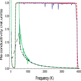
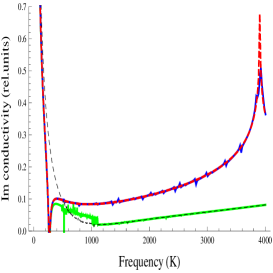
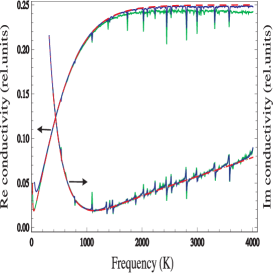
Figure S.3: Frequency dependencies of the real and imaginary parts of the massless Ohmic term of conductivity at very small wave number $q=10^{-8}|\vec{K}_{A}|$ in rel. units $e^{2}/\hbar$; a cutting parameter $q_{max}=0.14~{}K_{A}$. The model Falkovsky ; Falkovsky2008PhysUspekhi is simulated at T=3K, chemical potential $\mu=135$K (red dashed lines in figures (a–b)) and at T=200K, $\mu=33$K (red dashed line in figure (c)). Numerical results for our model are green-solid and black-dashed lines for the first-order approximation (with zero gauge-phases) (III.9) at T=3K, $\mu=135$K and T=200K, $\mu=33$K respectively, and blue line for the second-order approximation (with non-zero gauge-phases) (III.19) at T=3K, $\mu=135$K in figures (a–b). (c) Dependence of the real and imaginary parts of the massless Ohmic term of conductivity on a damping $\gamma$ for the second-order approximation (III.19) with $\gamma=0.1$ (green curve) and $\gamma=1$ (blue curve) at T=200K, $\mu=33$K.

According to the Table 1, the Fermi velocity $v_{M}$ for our model of massless Majorana energy states decrease in a factor higher than two for high wave numbers $q$ in respect to its value in the Dirac point. Therefore, the range $q$, $q<\omega_{max}/v_{M}$, $\omega_{max}<$1 eV increases in a factor two compared to the massless Dirac fermions. Since $q<0.28~{}K_{A}-0.56~{}K_{A}$ for our model, the range of integration over momentum $|q|<0.44~{}|K_{A}|$ is appropriate one and for it $\omega_{max}>7000$ K.

In the first-order approximation with zero-phases of the gauge fields, the analytical formulas for the integrands in separate conductivity contribution terms have been used. The integrals have been calculated with adaptive integration steps in both directions ($|k|,\phi$) providing high calculation accuracy (not less than 0.01%).

In the second order approximation with nonzero-phases of the gauge fields, we have to calculate numerically by introducing into consideration a small positive damping constant $\gamma$ for the states as a small imaginary contribution to the energies. The values of $\gamma$ define the extend of smoothness of the singular behaviour of integrand and does not influence on the general form of the dependency curve in accordance to fig. S.3c.

All quantities necessary for calculation of the complex conductivity have been calculated on a grid in the space of wave vectors with 200 discretization in angle $\phi$ for every given wave number $q$ and variable step (a denser grid at small wave numbers and larger at large ones) to the maximum wave number $q_{max}=0.44|K_{A}|$. 2D interpolation on this grid has been used to integrands evaluation in the intermediate points that is necessary for conductivity simulations. An error stipulated by the interpolation from the grid in wave vectors space has been roughly estimated by interpolation of the conic spectrum of Dirac pseudo-fermion model on the same lattice with subsequent usage of the interpolation data for evaluation of the conductivity. Its value turns out to be less than $10^{-3}$% .

Total estimation of the conductivity error has been performed by variation of the number of points used for interpolation of the energy band spectrum (by diminishing this number at factor two and subsequent comparison of the simulation results in both cases). It turns out to be not exceeding 10% in the considered frequency region. It should be noted that the error bars for values of the Fermi velocity which was measured by different techniques including transport experiments (Shubnikov – de Haas oscillations) NatPhys7-2011Elias , infrared measurements of the Pauli blocking in graphene Z.Q.Li_et_al_Nature Phys.4_532(2008) , magneto-optics magneto_optics_Fermi_velocity_NatCommun2014 , were also of the order of 10% .

References

- (1) Y. Luo, R.D. McDonald, P.F.S. Rosa, B. Scott, N. Wakeham, N.J. Ghimire, E.D. Bauer, J.D. Thompson, F. Ronning. Anomalous electronic structure and magnetoresistance in TaAs2. Sci. Rep. 6, 27294 (2016). doi 10.1038/srep27294
- (2) Q. Li et al. Chiral magnetic effect in ZrTe5. Nat. Phys. 12, 550 554 (2016).
- (3) J. Du, H. Wang, Q. Chen, Q. Mao, R. Khan, B. Xu, Yu. Zhou, Ya. Zhang, J. Yang, B. Chen, et al. Large unsaturated positive and negative magnetoresistance in Weyl semimetal TaP. Sci. China Phys. Mech. Astron. 59(5), 1 (2016).
- (4) X. Yan, Ch. Zhang, Sh.-Sh. Liu, Ya.-W. Liu, D.W. Zhang, F.-X. Xiu, P. Zhou. Two-carrier transport in SrMnBi2 thin films. Front. Phys. 12(3), 127209 (2017). DOI 10.1007/s11467-017-0663-0
- (5) H.-Zh. Lu, Sh.-Q. Shen. Quantum transport in topological semimetals under magnetic fields. Front. Phys. 12(3), 127201 (2017). DOI: 10.1007/s11467-016-0609-y
- (6) D.R. Cooper, B. D Anjou, N. Ghattamaneni, B. Harack, M. Hilke, A. Horth, N. Majlis, M. Massicotte, L. Vandsburger, E. Whiteway, V. Yu. Experimental Review of Graphene. ISRN Condensed Matter Physics. Vol.2012, Article ID 501686 (2012). doi:10.5402/2012/501686
- (7) K.I. Bolotin, K.J. Sikes, Z. Jiang, M. Klima, G. Fudenberg, J. Hone, P. Kim, H.L. Stormer. Ultrahigh electron mobility in suspended graphene. Solid State Communications. 146, 351 355 (2008).
- (8) Zh. Wang, H. Weng, Qu. Wu, X. Dai, Zh. Fang. Three-dimensional Dirac semimetal and quantum transport in Cd3As2. Phys. Rev. B 88(12), 125427 (2013).
- (9) T. Liang, Qu. Gibson, M.N. Ali, M. Liu, R.J. Cava, N.P. Ong. Ultrahigh mobility and giant magnetoresistance in the Dirac semimetal Cd3As2. Nature materials. 14(3), 280 284 (2015).
- (10) D.T. Son, B.Z. Spivak. Chiral anomaly and classical negative magnetoresistance of Weyl metals. Phys. Rev. B 88(10), 104412 (2013).
- (11) H. Huang et al. Graphene damage effects on radiation-resistance and configuration of copper-graphene nanocomposite under irradiation: A molecular dynamics study. Sci. Rep. 6, 39391 (2016). doi: 10.1038/srep39391
- (12) X. Huang, L. Zhao, Yu. Long, P. Wang, D. Chen, Zh. Yang, H. Liang, M. Xue, H. Weng, Zh. Fang, X. Dai, G. Chen. Observation of the chiral-anomaly-induced negative magnetoresistance in 3D Weyl semimetal TaAs. Phys. Rev. X5, 031023 ( 2015).
- (13) D. Xiao, M.-Ch. Chang, Q. Niu. Berry phase effects on electronic properties. Rev. Mod. Phys. 82, no. 3, 1959-2007 (2010). DOI:10.1103/RevModPhys.82.1959
- (14) R.V. Gorbachev, J.C. W. Song, G.L. Yu, A.V. Kretinin, F. Withers, Y. Cao, A. Mishchenko, I.V. Grigorieva, K.S. Novoselov, L.S. Levitov, A.K. Geim. Detecting topological currents in graphene superlattices. Science. 346, no. 6208, 448-451 (2014). DOI: 10.1126/science.1254966
- (15) P. San-Jose, J.L. Lado, R. Aguado, F. Guinea, J. Fernández-Rossier. Majorana Zero Modes in Graphene. Phys. Rev. X. 5, 041042 (2015).
- (16) P.A. Lee. From high temperature superconductivity to quantum spin liquid: progress in strong correlation physics. Rep. Prog. Phys. Vol. 71, 012501 (2008).
- (17) L.-H. Wu, Q.-F. Liang, X. Hu. New scheme for braiding Majorana fermions. Sci. Technol. Adv. Mater. 15, 064402 (2014).
- (18) A.Y. Kitaev. Unpaired Majorana fermions in quantum wires. Physics Uspekhi. 44(10S), 131 (2001).
- (19) G.W. Semenoff, P. Sodano. Stretched quantum states emerging from a Majorana medium. J. Phys. B. Vol. 40, 1479 1488 (2007).
- (20) G.W. Semenoff, P. Sodano. Stretching the Electron as Far as it Will Go. El.J.Theor.Phys. Vol. 3, no. 10, 157-190 (2006).
- (21) Fr. Wilczek. Chapter 14: Majorana and Condensed Matter Physics. In: The Physics of Ettore Majorana. (Cambridge University Press, Cambridge, UK, 2014).
- (22) S. Nadj-Perge, I.K. Drozdov, J. Li, H. Chen, S. Jeon, Ju. Seo, A.H. MacDonald, B.A. Bernevig, A. Yazdani. Observation of Majorana fermions in ferromagnetic atomic chains on a superconductor. Science. 346, 602 (2014). DOI: 10.1126/science.1259327
- (23) E. Majorana. A symmetric theory of electrons and positrons. I Nuovo Cimento. 14, 171-184 (1937).
- (24) C. Nayak, S.H. Simon, A. Stern, M. Freedman, S. Das Sarma. Non-abelian anyons and topological quantum computation. Rev. Mod. Phys. 80, 1083 (2008).
- (25) L.H. Kauffman, S.J. Lomonaco Jr. Braiding With Majorana Fermions. Reprint. arXiv:1603.07827v1 [cond-mat.str-el] 25 Mar 2016
- (26) A.A. Zyuzin, R.P. Tiwari. Intrinsic anomalous Hall effect in type-II Weyl semimetals. JETP Letters. 103, no. 11, 717 722 (2016).
- (27) Ch.-K. Chiu, Gu. Bian, H. Zheng, J. Yin, S.S. Zhang, S.-Y. Xu, M.Z. Hasan. Chiral Majorana Fermion Modes on the Surface of Superconducting Topological Insulators. Preprint arXiv:1612.09276v1 [cond-mat.supr-con] 29 Dec 2016
- (28) S. Backens, A. Shnirman, Y. Makhlin, Yu. Gefen, J.E. Mooij, G. Schön. Emulating Majorana fermions and their braiding by Ising spin chains. Reprint. arXiv:1703.08224v2 [cond-mat.mes-hall] 21 Apr 2017.
- (29) G.W. Semenoff, Condensed-matter simulation of a three-dimensional anomaly. Phys. Rev. Lett. 53, 2449 (1984).
- (30) K.S. Novoselov, A.K. Geim, S.V. Morozov, D.Jiang, Y. Zhang, M.I. Katsnelson, I.V. Grigorieva, S.V. Dubonos, A.A. Firsov. Two-dimensional gas of massles Dirac fermions in graphene. Nature. 438, 197-200 (2005).
- (31) A.H. Castro Neto et al., The electronic properties of graphene. Rev. Mod. Phys. 81, 109 (2009).
- (32) Z.K. Liu et al. Discovery of a three-dimensional topological Dirac semimetal, Na3Bi. Science. 343, 864 (2014).
- (33) S.-Y. Xu et al. Observation of Fermi arc surface states in a topological metal. Science. 347, 294 (2015).
- (34) M. Neupane et al. Observation of a three-dimensional topological Dirac semimetal phase in high-mobility Cd3As2. Nat. Commun. 5, 3786 (2014).
- (35) S. Borisenko, Qu. Gibson, D. Evtushinsky, V. Zabolotnyy, Bernd Büchner, R.J. Cava. Experimental realization of a three-dimensional Dirac semimetal. Phys. Rev. Lett. Vol. 113, 027603 (2014).
- (36) S. Jeon, B.B. Zhou, A. Gyenis, B.E. Feldman, I. Kimchi, A.C. Potter, Q.D. Gibson, R.J. Cava, A. Vishwanath, A. Yazdani. Landau quantization and quasiparticle interference in the three-dimensional Dirac semimetal Cd3As2. Nature Materials. 13, 851 (2014).
- (37) E. Pessa. The Majorana Oscillator. Electr. J. Theor. Phys. 3, 285 292 (2006).
- (38) H. Grushevskaya, G. Krylov. Massless Majorana-Like Charged Carriers in Two-Dimensional Semimetals. Symmetry. 8, 60 (2016). doi:10.3390/sym8070060
- (39) H. Hübener, M.A. Sentef, U. De Giovannini, A.F. Kemper, A. Rubio. Creating stable Floquet Weyl semimetals by laser-driving of 3D Dirac materials. Nature Communications. 8, 13940 (2017). DOI: 10.1038/ncomms13940
- (40) H.-Zh. Lu, Sh.-Q. Shen. Quantum transport in topological semimetals under magnetic fields. Front. Phys. 12(3), 127201 (2017). DOI 10.1007/s11467-016-0609-y
- (41) S.-Y. Xu et al. Discovery of a Weyl Fermion Semimetal and Topological Fermi Arcs. Science. Vol. 349, 613 (2015).
- (42) B. Q. Lv et al. Experimental Discovery of Weyl Semimetal TaAs. Phys. Rev. X. Vol. 5, 031013 (2015).
- (43) Lv, B. et al. Observation of Weyl nodes in TaAs. Nat. Phys. Vol. 11, 724 727 (2015). doi:10.1038/nphys3426
- (44) S.-Y. Xu et al.Discovery of a Weyl fermion state with Fermi arcs in niobium arsenide. Nat. Phys. 11, 748 (2015).
- (45) L. Yang et al. Weyl semimetal phase in the non-centrosymmetric compound TaAs. Nat. Phys. 11, 728 (2015). doi:10.1038/nphys3425
- (46) M.Z. Hasan, Su-Yang Xu, I. Belopolski, Sh.-M. Huang. Discovery of Weyl Fermion Semimetals and Topological Fermi Arc States. Annual Rev. Cond. Matt. Phys. 8, online on February 6, 2017 (2017). DOI: 10.1146/annurev-conmatphys-031016-025225
- (47) D.-F. Xu, Y.-P. Du, Zh. Wang, Yu.-P. Li, X.-H. Niu, Qi Yao, P. Dudin, Zh.-A. Xu, X.-G. Wan, D.-L. Feng. Observation of Fermi Arcs in Non-Centrosymmetric Weyl Semi-Metal Candidate NbP. Chin. Phys. Lett. 32, 107101 (2015).
- (48) Y. Li, F.D.M. Haldane. Topological Nodal Cooper Pairing in Doped Weyl Semimetals. arXiv.org/abs/1510.01730v3 (2015).
- (49) G. Chang, S.-Y. Xu, H. Zheng, B. Singh, Ch.-H. Hsu, Gu. Bian, N. Alidoust, I. Belopolski, D.S. Sanchez, S. Zhang, H. Lin, M.Z. Hasan. Room-temperature magnetic topological Weyl fermion and nodal line semimetal states in halfmetallic Heusler Co2TiX (X=Si, Ge, or Sn). Scientific Reports. 6, 38839 (2016). DOI: 10.1038/srep38839.
- (50) B. Roy. Interacting line-node semimetal and spontaneous symmetry breaking. Preprint. arXiv:1607.07867v1 [cond-mat.mes-hall] 26 Jul 2016.
- (51) Yo.Kim, B.J. Wieder, C.L. Kane, A.M. Rappe. Dirac Line Nodes in Inversion-Symmetric Crystals. Phys.Rev.Lett. Vol. 115, 036806 (2015).
- (52) Ch. Fang, Yi. Chen, H.-Yo. Kee, L. Fu. Topological nodal line semimetals with and without spin-orbital coupling. Phys. Rev. B. 92, 081201(R) (2015).
- (53) Gu. Bian, T.-R. Chang, R. Sankar, S.-Ya. Xu, H. Zheng, T. Neupert, Ch.-K. Chiu, Sh.-M. Huang, Gu. Chang, I. Belopolski, D.S. Sanchez, M. Neupane, N. Alidoust1, Ch. Liu, B.K. Wang, Ch.-Ch. Lee, H.-T. Jeng, Ch. Zhang, Zh. Yuan, Sh. Jia, A. Bansil, F. Chou, H. Lin, M.Z. Hasan. Topological nodal-line fermions in spin-orbit metal PbTaSe2. Nature Communications. 7, 10556 (2016) DOI: 10.1038/ncomms10556
- (54) B. Bradlyn, J. Cano, Zhijun Wang, M.G. Vergniory, C. Felser, R.J. Cava, B.A. Bernevig. Beyond Dirac and Weyl fermions: Unconventional quasiparticles in conventional crystals. Science. Vol. 353(6299), aaf5037 (2016). doi: 10.1126/science.aaf5037.
- (55) B.J. Wieder, Youngkuk Kim, A.M. Rappe, C.L. Kane. Double Dirac Semimetals in Three Dimensions. Phys. Rev. Lett. Vol. 116,186402 (2016).
- (56) L. Muechler, A. Alexandradinata, T.Neupert, R. Car. Topological Nonsymmorphic Metals from Band Inversion. Phys. Rev. X. 6, 041069 (2016).
- (57) Sh.-Y. Yang, Hao Yang, E. Derunova, S.S.P. Parkin, Binghai Yan, M.N. Ali. Symmetry demanded topological nodal-line materials. Preprint ArXiv:1707.04523v2 [cond-mat.mtrl-sci] 28 Jul 2017.
- (58) M. Hirayama, R. Okugawa, T. Miyake, Sh. Murakami. Topological Dirac nodal lines and surface charges in fcc alkaline earth metals. Nature Communications. 8, 14022 (2017) DOI: 10.1038/ncomms14022.
- (59) H. Weng, Yu. Liang, Q. Xu, R. Yu, Zh. Fang, X. Dai, Yo. Kawazoe. Topological node-line semimetal in three-dimensional graphene networks. Phys. Rev. B 92(4), 045108 (2015).
- (60) A.A. Burkov, M.D. Hook, L. Balents. Topological nodal semimetals. Phys. Rev. B 84(23), 235126 (2011). doi:10.1103/PhysRevB.84.235126
- (61) G. Bian, T.-R. Chang, H. Zheng, S. Velury, S.-Y. Xu, T. Neupert, C.-K. Chiu, S.-M. Huang, D. S. Sanchez, I. Belopolski, N. Alidoust, P.-J. Chen, G. Chang, A. Bansil, H.-T. Jeng, H. Lin, M. Z. Hasan. Drumhead surface states and topological nodalline fermions in TlTaSe2. Phys. Rev. B 93, 121113 (2016). doi:10.1103/PhysRevB.93.121113
- (62) Y.-H. Chan, C.-K. Chiu, M. Y. Chou, A. P. Schnyder, Ca3P2 and other topological semi-metals with line nodes and drumhead surface states. Phys. Rev. B 93, 205132 (2016). doi:10.1103/PhysRevB.93.205132
- (63) T.T. Heikkilä, G.E. Volovik. Dimensional crossover in topological matter: evolution of the multiple Dirac point in the layered system to the flat band on the surface. JETP lett. 93(2), 59 (2011).
- (64) N. Marzari, A.A. Mostofi, J.R. Yates, I. Souza, D. Vanderbilt. Rev. Mod. Phys. 84, 1419 (2012).
- (65) Q. Xu, R. Yu, Zh. Fang, X. Dai, H. Weng. Topological Nodal Line Semimetals in CaP3 family of materials. Phys.Rev. B 95, 045136 (2017). DOI: https://doi.org/10.1103/PhysRevB.95.045136
- (66) N.B. Kopnin, T.T. Heikkilä, G.E. Volovik. High-temperature surface superconductivity in topological flat-band systems. Phys. Rev. B 83(22), 220503 (2011).
- (67) T.T. Heikkilä, N.B. Kopnin, G.E. Volovik. Flat bands in topological media. JETP lett. 94(3), 233 (2011).
- (68) Ch.-L. Zhang, Zh. Yuan, Gu. Bian, S.-Ya. Xu, X. Zhang, M.Z. Hasan, Sh. Jia. Superconducting properties in single crystals of the topological nodal semimetal PbTaSe2. Phys. Rev. B. Vol. 93, 054520 (2016).
- (69) P.H. Ginsparg, K.G. Wilson. Phys. Rev. D 25, 2649(1982).
- (70) P.J. Moran, D.B. Leinweber, J.B. Zhang. Wilson mass dependence of the overlap topological charge density. Phys. Lett. B. 695, 337 342 (2011).
- (71) D.B. Kaplan, S. Sun. Phys. Rev. Lett. 108, 181807(4) (2012).
- (72) O. Vafek, A. Vishwanath. Dirac Fermions in Solids from High Tc cuprates and Graphene to Topological Insulators and Weyl Semimetals. Reprint. arXiv:1306.2272v1 [cond-mat.mes-hall] 10 Jun 2013
- (73) H. Zhang et al. Nature Physics 5, 438 (2009).
- (74) C.-X. Liu et al. Phys. Rev. B 82, 045122(19) (2010).
- (75) L. Fu, C.L. Kane. Phys. Rev. B 76, 045302(17) (2007).
- (76) Ch. Fang, H. Weng, X. Dai, Zh. Fang. Topological nodal line semimetals. arXiv:1609.05414v1 [cond-mat.mes-hall] 18 Sep 2016.
- (77) H. Huang, J. Liu, D. Vanderbilt, W. Duan. Topological nodal-line semimetals in alkaline-earth stannides, germanides, and silicides. Phys. Rev. B. 93, 201114(R) (2016).
- (78) A. Narayan. Tunable point nodes from line-node semimetals via application of light. Phys. Rev. B. Vol. 94, 041409(R) (2016).
- (79) H. Weng, X. Dai, Zh. Fang. Topological nodal line semimetals Chinese Phys. B. 25, 117106 (2016). doi.org/10.1088/1674-1056/25/11/117106.
- (80) V. Kozii, J.W.F. Venderbos, Liang Fu. Three-dimensional Majorana fermions in chiral superconductors. Sci. Adv. 2, e1601835 (2016).
- (81) C. Putzke, L. Malone, S. Badoux, B. Vignolle, D. Vignolles, W. Tabis, Ph. Walmsley, M. Bird, N.E. Hussey, C. Proust, A. Carrington. Inverse correlation between quasiparticle mass and Tc in a cuprate high-Tc superconductor. Sci. Adv. 2, e1501657 (2016). doi: 10.1126/sciadv.1501657
- (82) H.B. Nielsen, M. Ninomiya. The Adler-Bell-Jackiw anomaly and Weyl fermions in a crystal. Phys. Lett. B 130, 389 (1983).
- (83) L. Fu, C.L. Kane. Superconducting Proximity Effect and Majorana Fermions at the Surface of a Topological Insulator. Phys.Rev.Lett. 100, 096407 (2008). DOI:10.1103/PhysRevLett.100.096407
- (84) Shuang Jia, S.-Y. Xu, M.Z. Hasan. Weyl Semimetals, Fermi Arcs and Chiral Anomalies. Nature Materials. 15, 1140 1144 (2016). doi:10.1038/nmat4787
- (85) R. Yu, Z. Fang, X. Dai, Hongming Weng. Topological nodal line semimetals predicted from first principles calculations. Front. Phys. 12, 127202 (2017)
- (86) Y. Cao et al. Mapping the orbital wavefunction of the surface states in three-dimensional topological insulators. Nat. Phys. 9, 499 504 (2013).
- (87) H. Zhang, C.-X. Liu, S.-C. Zhang. Spin-orbital texture in topological insulators. Phys. Rev. Lett. 111, 066801 (2013).
- (88) Z.-H. Zhu et al. Layer-by-layer entangled spin-orbital texture of the topological surface state in Bi2Se3. Phys. Rev. Lett. 110, 216401 (2013).
- (89) H.B. Nielsen, M. Ninomiya. Absence of neutrinos on a lattice:(i). proof by homotopy theory. Nuclear Physics B. 185(1), 20 (1981).
- (90) H.B. Nielsenand, M. Ninomiya. Absence of neutrinos on a lattice: (ii). intuitive topological proof. Nuclear Physics B. 193(1), 173 (1981).
- (91) I. Montvay, G. Munster. Quantum Fields on a Lattice. (Cambridge University Press, UK, 1997).
- (92) J.M. Kosterlitz, D.J. Thouless. Ordering, metastability and phase transitions in two-dimensional systems. J. Phys. C. 6(7), 1181 (1973).
- (93) J. M. Kosterlitz, D.J. Thouless. Long range order and metastability in two dimensional solids and superfluids.(Application of dislocation theory). J. Phys. C. 5(11), L124, (1972).
- (94) F.C. Zhang, C. Gros, T.M. Rice, H Shiba. A renormalized hamiltonian approach to a resonant valence bond wavefunction. Supercond. Sci. Technol. 1, 36 (1988).
- (95) R. Shankar, N. Read. The nonlinear sigma model is massless. Nuclear Physics B. 336(3), 457, (1990).
- (96) F.D.M. Haldane. Continuum dynamics of the 1-D Heisenberg antiferromagnet: Identification with the O(3) nonlinear sigma model. Physics Lett. A. 93(9), 464 (1983).
- (97) F.D.M. Haldane. Nonlinear Field Theory of Large-Spin Heisenberg Antiferromagnets: Semiclassically Quantized Solitons of the One-Dimensional Easy-Axis Neel State. Phys. Rev. Lett. 50(15), 1153 (1983).
- (98) S.L. Sondhi, S.M. Girvin, J.P. Carini, D. Shahar. Continuous quantum phase transitions. Rev. Mod. Phys. 69, 315 (1997).
- (99) Fr. Pollmann, A.M. Turner, Erez Berg, M. Oshikawa. Entanglement spectrum of a topological phase in one dimension. Phys. Rev.B. 81(6), 064439 (2010).
- (100) B. Hunt, J. D. Sanchez-Yamagishi, A. F. Young, M. Yankowitz, B. J. LeRoy, K. Watanabe, T. Taniguchi, P. Moon, M. Koshino, P. Jarillo-Hererro, R. C. Ashoori. Massive Dirac fermions and Hofstadter butterfly in a van der Waals heterostructure. Science. 340, 1427 1430 (2013).
- (101) S. Wu, L. Wang, Yo. Lai, W.-Yu Shan, G. Aivazian, X. Zhang, T. Taniguchi, K. Watanabe, D. Xiao, C. Dean, Ja. Hone, Zh. Li, X. Xu. Multiple hot-carrier collection in photo-excited graphene Moiré superlattices. Sci. Adv. 2, e1600002 (2016). doi: 10.1126/sciadv.1600002
- (102) P.W. Anderson. Mater. Res. Bull. 8, 153 (1973).
- (103) P. Fazekas, P. Anderson. Phil. Mag. 30, 432 (1974).
- (104) I. Affleck, J.B. Marston. Phys. Rev. B 373, 774 (1988).
- (105) L.I. Hurski, H.V. Grushevskaya, N.A. Kalanda Nonadiabatic paramagnetic model of the pseudogap state in high-temperature cuprate superconductors, Proc. National Acad. of Science of Belarus, 54, 55 (2010).
- (106) S. Sachdev. Phys. Rev.B 45, 389 (1992).
- (107) N. Nagaosa, P.A. Lee Phys. Rev.B 45, 966 (1992).
- (108) X.-G. Wen, P.A. Lee. Phys. Rev. Lett. 76 503 (1996).
- (109) T. Hsu, J.B. Marston, I. Affleck. Phys. Rev.B 43, 2866 (1991).
- (110) S.A. Kivelson, D.S. Rokhsar, J.P. Sethna. Phys. Rev.B 35, 8865 (1987).
- (111) O. Vafek, Z. Tesanovic, M. Franz. Phys. Rev. Lett. 89, 157003 (2002).
- (112) D. Lee, I. Herbut. Phys. Rev.B 66, 904512 (2002).
- (113) M. Hermele, T. Senthil, M.P.A. Fisher, P.A. Lee, N. Nagaosa, X.-G. Wen. Stability of U(1) spin liquids in two dimensions. Phys.Rev.B 70, 214437 (2004).
- (114) N. Read, D. Green. Phys. Rev. B. 61, 10267 (2000).
- (115) D.A. Ivanov. Phys. Rev. Lett. 86, 268 (2001).
- (116) A. Stern, F. von Oppen, E. Mariani. Phys. Rev. B 70, 205338 (2004).
- (117) M. Stone, S.B. Chung. Fusion rules and vortices in superconductors. Phys. Rev. B. 73, 014505 (2006).
- (118) A. Abrikosov, L. Gorkov, I. Dzyaloshinskii. Quantum Field Theoretical Method in Statistical Physics. (Pergamon, Oxford, 1965).
- (119) M. Oshikawa. Phys. Rev. Lett. 84, 3370 (2000).
- (120) A. Paramekanti, A. Vishwanath. Phys. Rev.B 70, 245118 (2004).
- (121) A. Jaffe, F.L. Pedrocchi. Annales Henri Poincaré. 16, 189 (2015).
- (122) C.M. Bender, P.D. Mannheim. Phys. Lett. A. 374, 1616 (2010).
- (123) Z.C. Wei, C. Wu, Y. Li, Sh. Zhang, T. Xiang. Majorana Positivity and the Fermion Sign Problem of Quantum Monte Carlo Simulations. Preprint arXiv:1601.01994v4 [cond-mat.str-el] 3 Jun 2016
- (124) E.J. Cussen, D.R. Lynham, J. Rogers. Magnetic order arising from structural distortion: Structure and magnetic properties of Ba2LnMoO6. Chem. Mater. 18, 2855 2866 (2006).
- (125) T. Aharen et al. Magnetic properties of the geometrically frustrated S= 1/2 antiferromagnets La2LiMoO6 and Ba2YMoO6, with the B-site ordered double perovskite structure: Evidence for a collective spin-singlet ground state. Phys. Rev. B. 81, 224409 (2010).
- (126) M.A. de Vries, A.C. Mclaughlin, J-W. G. Bos. Valence bond glass on an fcc lattice in the double perovskite Ba2YMoO6. Phys. Rev. Lett. 104, 177202 (2010).
- (127) J.P. Carlo et al. Triplet and in-gap magnetic states in the ground state of the quantum frustrated fcc antiferromagnet Ba2YMoO6. Phys. Rev. B 84, 100404 (2011).
- (128) A.J. Steele, P.J. Baker, T. Lancaster, F.L. Pratt, I. Franke, S. Ghannadzadeh, P.A. Goddard, W. Hayes, D. Prabhakaran, S.J. Blundel. Low-moment magnetism in the double perovskites BaOsO6( Li, Na). Phys. Rev. B 84, 144416 (2011).
- (129) Lei Xu, N.A. Bogdanov, A. Princep, P. Fulde, J. van den Brink, L. Hozoi. Covalency and vibronic couplings make a nonmagnetic =3/2 ion magnetic. npj Quantum Materials. 1, 16029 (2016). doi:10.1038/npjquantmats.2016.29
- (130) J.A. Waugh, Th. Nummy, St. Parham, Qihang Liu, Xiuwen Zhang, A. Zunger, D.S. Dessau. Minimal ingredients for orbital-texture switches at Dirac points in strong spin orbit coupled materials. npj Quantum Materials. 1, 1 6025 (2016). doi:10.1038/npjquantmats.2016.25
- (131) G.G. Krylov, H.V. Krylova, M.A. Belov. Electronic transport in low-dimensional systems: localization effects. In: Dynamical Phenomena in Complex Systems, eds. A.V. Mokshin et al. (MOiN RT Publishing, Kazan, 2011). P.161–180. (in Russian)
- (132) H.V. Grushevskaya, G.G. Krylov. Electronic structure and transport in graphene: quasi-relativistic Dirac–Hartre–Fock self-consistent field approximation. Preprint arXiv:1309.1847v1 [cond-mat.mes-hall] 7 Sep 2013
- (133) H.V. Grushevskaya, G.G. Krylov. Charge Carriers Asymmetry and Energy Minigaps in Monolayer Graphene: Dirac Hartree Fock approach. Int. J. Nonlinear Phen. in Comp. Sys. 16, 189-208 (2013).
- (134) H.V. Grushevskaya, G. Krylov. Partially Breaking Pseudo-Dirac Band Symmetry in Graphene. J. Nonlin. Phen. in Complex Sys. 17, no. 1, 86–96 (2014).
- (135) H.V. Grushevskaya, G. Krylov. Quasi-relativistic calculus of graphene monolayer minimal conductivity. Preprint arXiv:1401.6880v1 [cond-mat.mes-hall] 24 Jan 2014.
- (136) H.V. Grushevskaya, G. Krylov. Quantum Field Theory of Graphene with Dynamical Partial Symmetry Breaking. J. Mod. Phys. 5, no. 10, 984-994 (2014).
- (137) H.V. Grushevskaya and G.G. Krylov. Chapter 3. Graphene: Beyond the Massless Dirac’s Fermion Approach. In: Nanotechnology in the Security Systems, NATO Science for Peace and Security Series C: Environmental Security, J. Bona and S. Kruchinin (eds.). (Springer Science+Business Media, Dordrecht, 2015). P. 21-31.
- (138) H.V. Grushevskaya, G. Krylov, V.A. Gaisyonok, D.V. Serow. Symmetry of Model N = 3 for Graphene with Charged Pseudo-Excitons. Int. J. Nonlin. Phenom. in Complex Sys. 18, no. 1, 81-98 (2015).
- (139) H.V. Grushevskaya, G. Krylov. Semimetals with Fermi Velocity Affected by Exchange Interactions: Two Dimensional Majorana Charge Carriers. J. Nonlin. Phenom. in Complex Sys. 18, no. 2, 266-283 (2015).
- (140) H.V. Grushevskaya, G.G. Krylov. Chapter 9. Electronic Structure and Transport in Graphene: QuasiRelativistic Dirac-Hartree-Fock Self-Consistent Field Approximation. In: Graphene Science Handbook: Electrical and Optical Properties. Vol. 3. Eds. M. Aliofkhazraei, N. Ali, W.I. Milne, C.S. Ozkan, S. Mitura, J.L. Gervasoni. (Taylor and Francis Group, CRC Press, USA, UK, 2016). Pp. 117-132.
- (141) H.V. Grushevskaya, G.G. Krylov. Low frequency conductivity in monolayer graphene model with partial unfolding of Dirac bands. Int. J. Mod. Phys. 30, 1642009 (2016).
- (142) L.C. Lew Yan Voon, M.n Willatzen. The k-p method : electronic properties of semiconductors. (Springer-Verlag, Berlin, Heidelberg, 2009).
- (143) J.M. Luttinger, W. Kohn. Motion of electrons and holes in perturbed periodic fields. Phys. Rev. 97(4), 869 (1955).
- (144) G. Dresselhaus, A.F. Kip, C. Kittel. Cyclotron resonance of electrons and holes in silicon and germanium crystals. Phys. Rev. 98(2), 368 (1955).
- (145) A. Kormányos, G. Burkard, M. Gmitra, J. Fabian, V. Zólyomi, N.D. Drummond, V. Fal ko. kp theory for two-dimensional transition metal dichalcogenide semiconductors. 2D Mater. 2, 022001 (2015).
- (146) Yo.-S. Lee, M.B. Nardelli, N. Marzari. Band Structure and Quantum Conductance of Nanostructures from Maximally-Localized Wannier Functions: The Case of Functionalized Carbon Nanotubes. Preprint arXiv:cond-mat/0507089v1 [cond-mat.mtrl-sci] 4 Jul 2005
- (147) A.A. Mostofi, J.R. Yates, Y.-S. Lee, I. Souza, D. Vanderbilt, N. Marzari. Wannier90: A Tool for Obtaining Maximally-Localised Wannier Functions. Comput. Phys. Commun. 178, 685 (2008).
- (148) Q. Xu, R. Yu, Zh. Fang, X. Dai, H. Weng. Topological Nodal Line Semimetals in CaP3 family of materials. Phys.Rev. B 95, 045136 (2017). DOI: https://doi.org/10.1103/PhysRevB.95.045136
- (149) Wallace, P. R. 1947. The Band Theory of Graphite. Phys.Rev. 71, no.9, 622-634.
- (150) G.V. Grushevskaya, L.I. Komarov, and L.I. Gurskii. Exchange and correlation interactions and band structure of non-close-packed solids. Physics of the solid state. 40, no. 11, 1802 - 1805 (1998).
- (151) H.V. Grushevskaya, L.I. Hurski, L.I. Komarov, G.G. Krylov Atomic ellipsoids as a form of deformed electron shells of solids. Proc. National Acad. of Science of Belarus 40, 58 (1996); H.V. Grushevskaya, L.I. Hurski, L.I. Komarov, G.G. Krylov Nonsphericity of electron density distribution and polarization effects in solids. Proc. National Acad. of Science of Belarus 40 49 (1996); H.V. Grushevskaya, L.I. Hurski, N.N. Dorozkhin . . , . . , . . . Method of Green’s functions for a crystal in a complex momentum-energy space: the case of nonspherical interatomic potential. Proc. National Acad. of Science of Belarus 42 55 (1998); H.V. Grushevskaya, L.I. Hurski, N.N. Dorozkhin Modeling of the correlation non-spherical potential of the interatomic interaction in solids. Proc. National Acad. of Science of Belarus 42 60 (1998).
- (152) S.Y. Zhou et al. Origin of the energy bandgap in epitaxial graphene. Nat. Mater. 7, 259 260 (2008).
- (153) H.V. Grushevskaya, G.G. Krylov. Non-Abelian Majorana-Like Quasi-Excitation in Dirac Materials. Int. J. Nonlinear Phenomena in Complex Systems. 20, 153 (2017).
- (154) S. Chakravarty, R.B. Laughlin, D.K. Morr, C. Nayak. Phys. Rev. B 64, 094503 (2002).
- (155) L. Lu, M. Song, W. Liu, A.P. Reyes, P. Kuhns, H.O. Lee, I.R. Fisher, V.F. Mitrović. Magnetism and local symmetry breaking in a Mott insulator with strong spin orbit interactions. Nat. Commun. 8, 14407 doi: 10.1038/ncomms14407 (2017).
- (156) J. Zak. Berry s phase for energy bands in solids. Phys. Rev. Lett. 62, 2747 2750 (1989).
- (157) J.K. Asbóth, L. Oroszlány, A. Pályi. A Short Course on Topological Insulators. Band Structure and Edge States in One and Two Dimensions. Lecture Notes in Physics. Vol. 919. (Springer International Publishing, Heidelberg, New York, 2016).
- (158) F. Wilczek, A. Zee. Appearance of Gauge Structure in Simple Dynamical Systems. Phys. Rev. Lett. 52, 2111 (1984).
- (159) M. Hirayama, R. Okugawa, T. Miyake, Sh. Murakami. Topological Dirac nodal lines and surface charges in fcc alkaline earth metals. Nature Communications. 8, 14022 (2017). DOI: 10.1038/ncomms14022
- (160) H. Krylova, L. Hurski. Spin polarization in strongly correlated systems. (LAP Lambert Academic Publishing, Saarbrucken, Germany, 2013).
- (161) A.A. Soluyanov, D. Gresch, Z. Wang, Q. Wu, M. Troyer, X. Dai, B.A. Bernevig. Type-II Weyl Semimetals. Nature (London). 527, 495-498 (2015).
- (162) J. Jiang, Z.K. Liu, Y. Sun, H.F. Yang, C.R. Rajamathi,Y.P.Qi, L.X. Yang, C. Chen, H. Peng, C.-C. Hwang, S.Z. Sun, S.-K. Mo, I. Vobornik, J. Fujii, S.S.P. Parkin, C. Felser, B.H. Yan, Y.L. Chen. Signature of type-II Weyl semimetal phase in MoTe2. Nature Communications. 8, 13973 (2017). DOI: 10.1038/ncomms13973
- (163) F. Bassani, G. Pastori Parravicini. Electronic States and Optical Transitions in Solids. (Pergamon Press, 1975).
- (164) V.D. Kraeft, D. Kremp, W. Ebeling, G. Röpke. Quantum statistics of charged particle systems. (Akademie-Verlag, Berlin, 1986).
- (165) E.A. Albanesi, E.L. Peltzer y Blanca, A.G. Petukhov. Calculated optical spectra of IV VI semiconductors PbS, PbSe and PbTe. Comput. Mater. Sci. 32, 85 (2005).
- (166) L.A. Falkovsky. Optical properties of graphene and IV-VI semiconductors. Physics-Uspekhi. 51, 887-897 (2008).
- (167) Y. Tokura et al. Phys. Rev. Lett. 70 2126 (1993).
- (168) A.S. Davydov. Quantum mechanics. (Science, Moscow, 1973).
- (169) F. Dyson. Advanced quantum mechanics. (World Scientific Publishing, Singapore, 2007).
- (170) M. Dirac. Lectures on Quantum Field Theory. (Belfer Graduate School of Science Series, Yeshiva University, New York, 1966)
- (171) H. Callen, R.H. Swendsen, R. Tahir-Kheli. Zero-frequency behavior of thermodynamic green’s functions. Phys. Lett. A25 505-506(1967)
- (172) H.V. Grushevskaya, L.I. Hurski. Coherent Charge Transport in Strongly Correlated Electron Systems: Negatively Charged Exciton Quantum Matter. 4, 384-386 (2015). Doi:10.1166/qm.2015.1211
- (173) R.R. Nair, P. Blake, A.N. Grigorenko, K.S. Novoselov, T.J. Booth, T. Stauber, N.M.R. Peres, A.K. Geim. Science. 320, 1308 (2008).
- (174) T. Ando, Y. Zheng, H. Suzuura. Dynamical conductivity and zero-mode anomaly in honeycomb lattices. J. Phys. Soc. Jpn. 71, 1318 - 1324 (2002).
- (175) L.A. Falkovsky, A.A. Varlamov. Space-time dispersion of graphene conductivity. Eur. Phys. J. B. 56, 281-284 (2007).
- (176) K. Ziegler. Minimal conductivity of graphene: Nonuniversal values from the Kubo formule. Phys. Rev. B. 75, 233407 (2007).
- (177) L.P. Kadanoff, G. Baym. Quantum statistical mechanics. (New York, 1962) [ . , . . . ( , 1964).
- (178) C. Itzykson, J.-B. Zuber. Quantum Field Theory. (Dover, New York, 2006).
- (179) Braid Group, Knot Theory and Statistical Mechanics. Eds. C.N. Yang and M.L. Ge. Advanced Series in Mathematical Physics, Vol. 9. (World Scientific, Singapore, 1991).
- (180) M.-L. Ge, L.-W. Yu. Yang Baxter equation, Majorana fermions and three body entangling states. Int. J. Mod. Phys. B 28, 1450089 (2014). DOI: 10.1142/S0217979214500891
- (181) D. Hsieh et al. Observation of unconventional quantum spin textures in topological Insulators. Science. 323, 919-922 (2009).
- (182) Zhi-Guo Chen, Zhiwen Shi, Wei Yang, Xiaobo Lu, You Lai, Hugen Yan, Feng Wang, Guangyu Zhang, Zhiqiang Li. Observation of an intrinsic bandgap and Landau level renormalization in graphene/boron-nitride heterostructures. Nature Communications. 5, 4461 (2014) DOI: 10.1038
- (183) I. Pletikosic, M. Kralj, P. Pervan, R. Brako, J.Coraux, A. T. N’Diaye, C. Busse, T. Michely. Dirac Cones and Minigaps for Graphene on Ir(111). Phys. Rev. Lett. 102, 056808 (2009), arXiv: 0807.2770v2 [cond-mat.mtrl-sci] 13 Feb2009.
- (184) C.R. Woods, L. Britnell, A. Eckmann, R.S. Ma, J.C. Lu, H.M. Guo, X. Lin, G.L. Yu, Y. Cao, R.V. Gorbachev, A.V. Kretinin, J. Park, L.A. Ponomarenko, M.I. Katsnelson, Yu.N. Gornostyrev, K. Watanabe, T. Taniguchi, C. Casiraghi, H-J. Gao, A.K. Geim, K.S. Novoselov. Commensurate–incommensurate transition in graphene on hexagonal boron nitride. Nature Physics. 10, 451-456 (2014). doi:10.1038/nphys2954
- (185) E.Y. Andrei, Guohong Li, Xu Du. Electronic properties of graphene: a perspective from scanning tunneling microscopy and magnetotransport. Rep. Prog. Phys. 75, 056501 (2012).
- (186) G. Li, A. Luican, J.M.B. Lopes dos Santos, A.H. Castro Neto, A. Reina, J. Kong, E.Y. Andrei. Observation of Van Hove singularities in twisted graphene layers. Nature Phys. 6, 109 (2009).
- (187) A. Mishchenko, J.S. Tu, Y. Cao, R.V. Gorbachev, J.R. Wallbank, M.T. Greenaway, V.E. Morozov, S.V. Morozov, M.J. Zhu, S.L. Wong, F. Withers, C.R. Woods, Y-J. Kim, K. Watanabe, T. Taniguchi, E.E. Vdovin, O. Makarovsky, T.M. Fromhold, V.I. Fal ko, A.K. Geim, L. Eaves, K.S. Novoselov. Twist-controlled resonant tunnelling in graphene/boron nitride/graphene heterostructures. Nature Nanotechnology. 9, 808-813 (2014).
- (188) P.M. Platzmann, P.A. Wolf. Waves and interactions in plasmas. (Benjamin, New York, 1973).
- (189) A.B. Mikhailovsky Theory of plasma instabilities Vol.2. (Atomizdat, Moscow, 1977).
- (190) K. S. Novoselov, A. K. Geim, S. V. Morozov et al. Electric field in atomically thin carbon films. Science. 306, 666 (2004).
- (191) K.I. Bolotin, K.J. Sikes, J.Hone, H.L. Stormer, P. Kim. Temperature-dependent transport in suspended graphene. Phys. Rev. Lett. 101, 096802 (2008).
- (192) X. Du, I. Skachko, A. Barker, E.Y. Andrei. Approaching ballistic transport in suspended graphene. Nature Nanotechnology. 3, 491 (2008).
- (193) C.R. Dean, A.F. Young, I. Meric et al. Boron nitride substrates for high-quality graphene electronics, Nature Nanotechnology. 5, 722 (2010).
- (194) S.-K. Yip. Kinetic equation and magneto-conductance for Weyl metal in the clean limit. Preprint, arXiv: 1508.01010
- (195) A.C. Niemann, J. Gooth, Sh.-Ch. Wu, et al. Chiral magnetoresistance in the Weyl semimetal NbP. Sci. Rep. 7, 43394 (2017). doi: 10.1038/srep43394
- (196) A. Das, Yu. Ronen, Yo. Most, Yu. Oreg, M. Heiblum, H. Shtrikman. Zero-bias peaks and splitting in an Al InAs nanowire topological superconductor as a signature of Majorana fermions. Nat. Phys. 8, 887 895 (2012). DOI: 10.1038/NPHYS2479
- (197) V. Mourik et al. Signatures of Majorana fermions in hybrid superconductor-semiconductor nanowire devices. Science. 336, 1003-1007 (2012).
- (198) M.T. Deng et al. Observation of majorana fermions in a Nb–InSb nanowire-Nb hybrid quantum device. Preprint at http://arxiv.org/abs/1204.4130 (2012).
- (199) C. Di Giorgio, F. Bobba, A.M. Cucolo, A. Scarfato, S.A. Moore, G. Karapetrov, D. D Agostino, V. Novosad, V. Yefremenko, M. Iavarone. Observation of superconducting vortex clusters in S/F hybrids. Scientific Reports. 6, 38557 (2016). DOI: 10.1038/srep38557
- (200) F. von Oppen, Ya. Peng, F. Pientka. Topological superconducting phases in one dimension. In: Topological Aspects of Condensed Matter Physics. (Oxford University Press, Oxford, 2017). DOI:10.1093/acprof:oso/9780198785781.003.0009
- (201) G. Koren, T. Kirzhner, E. Lahoud, K. B. Chashka, A. Kanigel. Proximity-induced superconductivity in topological Bi2Te2Se and Bi2Se3 films: Robust zero-energy bound state possibly due to Majorana fermions. Phys.Rev. B. 84, 224521 (2011). DOI: 10.1103/PhysRevB.84.22452]
- (202) T. Dirks, T.L. Hughes, S. Lal, B. Uchoa, Y.F. Chen, C. Chialvo, P.M. Goldbart, et al. Transport through Andreev bound states in a graphene quantum dot. Nature Physics. 7(5), 386-390 (2011).
- (203) A.I. Buzdin. Proximity effects in superconductor-ferromagnet heterostructures. Rev. Mod. Phys. 77, 935 976 (2005).
- (204) H. Goudarzi, M. Khezerlou, S. Asgarifar. Novel Majorana mode and magnetoresistance in ferromagnetic superconducting topological insulator. Physica E. 8̱7, 155 160 (2017). DOI:10.1016/j.physe.2016.12.002
- (205) Yang Peng, Falko Pientka, Yu. Vinkler-Aviv, L.I. Glazman, F. von Oppen. Robust Majorana conductance peaks for a superconducting lead. Phys.Rev.Lett. 115, 266804 (2015). DOI: 10.1103/PhysRevLett.115.266804
- (206) R. Yang, G. Yu. Anomalous differential conductance of In-Bi2Te3 contact. arXiv.org Preprint. arXiv:1103.0591v1 [cond-mat.mtrl-sci] (2011).
- (207) Z.Q. Li et al. Nature Phys. 4, 532 (2008).
- (208) Zh.-G. Chen, Zh. Shi, W. Yang, X. Lu, Yo. Lai, H. Yan, F. Wang, G. Zhang, Zh. Li. Observation of an intrinsic bandgap and Landau level renormalization in graphene/boron-nitride heterostructures. Nature Communications. 5, 4461 (2014). DOI: 10.1038/ncomms5461
- (209) L.A. Falkovsky. Optics of semiconductors with a linear electron spectrum. Low Temp. Phys. 37(6), 480 (2011). doi: 10.1063/1.3615524
- (210) D.C. Elias, R.V. Gorbachev, A.S. Mayorov, S.V. Morozov, A.A. Zhukov, P. Blake, L.A. Ponomarenko, I.V. Grigorieva, K.S. Novoselov, F. Guinea, A.K. Geim. Dirac cones reshaped by interaction effects in suspended graphene. Nat. Phys. 7, 701 (2011). doi:10.1038/nphys2049
- (211) M.E. Peskin, D.V. Schroeder, An Introduction to Quantum Field Theory (Addison-Wesley Publishing Company, New York, 1995).
- (212) A. Alexandradinata, X. Dai, B. A. Bernevig, Wilson-loop characterization of inversion-symmetric topological insulators. Phys. Rev. B 89, 155114 (2014). doi:10.1103/PhysRevB.89.155114
- (213) A. Alexandradinata, Z. Wang, B. A. Bernevig, Topological insulators from group cohomology. Phys. Rev. X 6, 021008 (2016)
- (214) V.A. Fock. Foundations of quantum mechanics. (Science Publishing Company, Moscow, 1976) (in Russian).