Abstract

We study observational viability of Natural Inflation with a tachyon field as inflaton. By obtaining the main perturbation parameters in this model, we perform a numerical analysis on the parameter space of the model and in confrontation with $68\%$ and $95\%$ CL regions of Planck2015 data. By adopting a warped background geometry, we find some new constraints on the width of the potential in terms of its height and the warp factor. We show that the Tachyon Natural Inflation in the large width limit recovers the tachyon model with a $\phi^{2}$ potential which is consistent with Planck2015 observational data. Then we focus on the reheating era after inflation by treating the number of e-folds, temperature and the effective equation of state parameter in this era. Since it is likely that the value of the effective equation of state parameter during the reheating era to be in the range $0\leq\omega_{eff}\leq\frac{1}{3}$, we obtain some new constraints on the tensor to scalar ratio, $r$, as well as the e-folds number and reheating temperature in this Tachyon Natural Inflation model. In particular, we show that a prediction of this model is $r\leq\frac{8}{3}\,\delta_{ns}$, where $\delta_{ns}$ is the scalar spectral tilt, $\delta_{ns}=1-n_{s}$. In this regard, given that from the Planck2015 data we have $\delta_{ns}=0.032$ (corresponding to $n_{s}=0.968$), we get $r\leq 0.085$.
PACS: 98.80.Bp, 98.80.Cq, 98.80.Es
Key Words: Natural Inflation, Tachyon Field, Reheating, Observational Constraints

1 Introduction

After introduction of “cosmological inflation” by Guth in 1981 [1], the idea of the rolling scalar field driving the dynamics of the early inflationary expansion was introduced by Linde [2] and Albrecht and Steinhardt [3]. Inflation models predict some small inhomogeneities (caused by the quantum fluctuations of the scalar field) leading eventually to the large scale structure formation in the Universe. It is also predicted that in a simple slow-roll inflation (defined by a canonical scalar field with a nearly flat potential) the dominant mode of the primordial density perturbations is almost adiabatic and nearly scale invariant with a Gaussian distribution [4, 5, 6, 7, 8, 9].

A problem with the inflation models is that the width of the potential must be much larger than its height, so that there will be a large number of e-folds of the scale factor to fit with the CMB anisotropy measurements. In fact, from Ref. [10] the ratio between the height and the fourth power of the width must fulfill

$$\frac{\Delta V}{(\Delta\phi)^{4}}\leq 10^{-6}$$ (1)

which means that the potential is almost flat. In this relation $\Delta$ shows the change in the corresponding parameters. In this regard, to address the theoretical problems of the rolling inflaton models, Freese, Frieman, and Olinto in 1990 have proposed the Natural Inflation (NI) scenario [11]. In the Natural Inflation, an axion-like particle (a pseudo-Nambu-Goldstone boson) is the field responsible for running of the inflation. A shift symmetry (that is, the potential is invariant under a transformation $\phi\rightarrow\phi+constant$) in the Natural Inflation ensures flatness of the potential [11, 12, 13]. Note that in this model the potential is “nearly” flat and eventually, after enough inflation, the symmetry is broken and the inflation phase terminates. Natural Inflation, in its simplest realization, has the following potential

$$V(\phi)=\Lambda^{4}\bigg{[}1+\cos\bigg{(}\frac{\phi}{f}\bigg{)}\bigg{]}.$$ (2)

The height of the potential is given by $2\Lambda^{4}$ and the width by $\pi f$. In fact, $f$ is an axion decay constant which parameterizes the spontaneous symmetry breaking scale needed to end the inflation phase. Actually, when a global symmetry is spontaneously broken in particle physics, Nambu-Goldstone bosons arise at a scale $f\sim m_{pl}$ (where $m_{pl}$ is the reduced Planck mass). However, when the shift symmetry is exact, the inflaton doesn’t roll and therefore inflation doesn’t happen. By an explicit symmetry breaking, the pseudo-Nambu-Goldstone bosons with “nearly flat” potential arise and inflation can happen. These bosons arise at a mass scale $m\sim\Lambda$ below the spontaneous symmetry breaking scale [14]. These two scales are important because they show the symmetry breaking’s scales. To constraint the values of $\Lambda$ and $f$, one can use the recent bounds on the scalar spectral index and tensor-to-scalar ratio from observational data.

In the original Natural Inflation (a canonical scalar field with cosine potential) and with $\Lambda\sim m_{GUT}\sim 10^{16}$ GeV, the pseudo-Nambu-Goldstone boson field runs inflation if $f\geq m_{pl}$. In this limit, the scalar spectral index and tensor-to-scalar ratio of the Natural Inflation are consistent with observational data. For $f\sim m_{pl}$ and considering $m_{pl}\sim 10^{19}$ GeV, we have the height-to-forth power of the width ratio as $\frac{\Lambda^{4}}{f^{4}}\sim 10^{-12}$ (which satisfies the condition (1)). In the $f\gg m_{pl}$ limit, $n_{s}$ and $r$ are independent of $f$ and for a given value of the number of e-folds there is a specific fixed point in $r-n_{s}$ plane. Actually, in this limit, Natural Inflation meets a large field $m^{2}\phi^{2}$ model. In this case, one gets $m_{\phi}\sim 10^{13}$ GeV [13, 15]. The authors of Ref. [56], by considering the new bounds on the scalar spectral index from Planck2015 and by studying the reheating phase with Natural potential, have obtained a new constraint on $f$ as $f>5.6\,m_{pl}$. The authors of Ref. [17] have studied the Hybrid Natural Inflation and by considering the energy scale of the inflation they have obtained some bounds on $f$ in some cases. See also [18, 19, 20] for other works on the Natural Inflation.

The mentioned works have considered a canonical scalar field with cosine potential. However, it is believed that there is a possibility that inflation may be driven by a single field where its kinetic energy is non-canonical. Such non-canonical models (usually referred as “k-inflation”) predict that the primordial density perturbations are somehow scale dependent (mildly supported by the Planck2015 observational data [21, 22]) and their distribution is non-Gaussian. Among the k-inflation models, we can mention the Tachyon inflation where the tachyon field is associated with the D-branes in string theory [23, 24, 25]. When this field rolls slowly down its potential, the Universe evolves smoothly from an accelerating expansion phase to a nonrelativistic fluid dominated era [26]. The tachyon, as a dark energy component, can be responsible for the late time cosmic speed-up of the Universe [27, 28, 29]. It can also be considered as the inflaton driving the initial cosmological inflation phase [30, 31]. Some aspects of tachyon field cosmology can be seen in [32, 33].

On the other hand, it has been shown that in a moving Dp-brane in the $k$ NS5-brane background (around a ring with radius $R$, where $k$ is the number of NS5-branes) the radion could be tachyonic. This is the idea of the geometrical tachyon [34, 35, 36, 37]. If one considers the solution inside the ring and uses a tachyon map, the potential of the tachyon would be of the cosine type as $V(\phi)=A\cos\left(\frac{\phi}{kl_{s}^{2}}\right)$ with $A=\frac{\tau R}{\sqrt{kl_{s}^{2}}}$ [36, 37]. Here $\tau$ is the tension of the Dp-brane, $R$ the radius of the ring and $l_{s}$ the string length. By comparing this potential with the potential in Natural Inflation we see that the string length is related to the width of the potential, and tension and radius are related to its height. Roughly speaking, we can take $kl_{s}^{2}\equiv f$ and $A\equiv\Lambda^{4}$.

Here we consider a tachyon field with a Natural potential as driver of cosmological inflation. Adopting the potential of the Natural Inflation is just like a constant shift in the “cosine” potential obtained by considering a probe Dp-brane in a NS5-brane ring background. Actually, one of the problems of the open string tachyon is that its potential should tend to zero as $\phi\rightarrow\infty$ in order that no D-brane and open string should exist at ground state [38, 39]. So, in this case there will be no reheating phase because the potential has a minimum at asymptotic infinity. However, by adopting the potential (2), we shall not encounter with this issue in the sense that in this case there would be a minimum at a finite value of $\phi$. As we shall see, Tachyon Natural Inflation (TNI) in the large $f$ limit approaches the tachyon model with $\phi^{2}$ potential which is consistent with the Planck2015 observational data. Note that the Planck2015 observational data rule out a canonical scalar field with $\phi^{2}$ potential. Actually, although the scalar spectral index of the canonical $\phi^{2}$ model is consistent with observation, its tensor-to-scalar ratio is out of the $95\%$ CL of the Planck2015 observational data. However, as we show, the tachyon $\phi^{2}$ model is consistent with the Planck2015 dataset. We study cosmological inflation and perturbations in a TNI model with warped background geometry (specified by the warp factor $\lambda$). By a numerical study of the scalar spectral index and the tensor-to-scalar ratio we obtain some new constraints on parameter $f$. The reason that we consider a warped background is that to have tachyon inflation with “steep potential” it is necessary that the background is warped [40]. We shall see that the bound on $f$ is not just in terms of $m_{pl}$, as it is in the canonical NI. In the TNI model, the constraints on $f$ depends on $m_{pl}$, $\lambda$ and $\Lambda$. This is because of the form of the energy density (and Friedmann equation) in the tachyon model.

Exploring the reheating process after the end of inflation is an important subject in studying the cosmic inflation. After the Universe inflates sufficiently and the slow-roll conditions break down, the inflation era terminates. By ending the inflation phase, the scalar field responsible for cosmic inflation starts to oscillate about the minimum of its potential. The simple canonical reheating scenario states that the inflaton loses its energy by oscillation and decays into a plasma of the relativistic particles (corresponding to a radiation dominated Universe) by entering the processes which include the physics of non-equilibrium phenomena and particle creation [41, 42, 43]. However, some other complicated scenarios of reheating including non-perturbative processes have been proposed by several authors. The tachyonic instability [44, 45, 46, 47, 48, 49], the instant preheating [50] and the parametric resonance decay [51, 52, 53] are some examples of the non-perturbative reheating scenarios which should be mentioned. One can characterize the reheating era dynamics by seeking for the reheating temperature ($T_{rh}$) and the number of e-folds during reheating ($N_{rh}$) which give some more constraints on the model parameters [54, 55, 56, 57, 58, 59]. The effective equation of state parameter during reheating ($\omega_{eff}$) is another important parameter which gives us some more useful information. Domination of the potential energy of the field over the kinetic energy gives $\omega_{eff}=-1$ and domination of the kinetic term over potential energy gives $\omega_{eff}=+1$. We assume the range of the effective equation of state parameter during the reheating phase to be given as $-\frac{1}{3}\leq\omega_{eff}\leq\frac{1}{3}$. This is because, we have $\omega_{eff}=-\frac{1}{3}$ at the end of the inflation era and $\omega_{eff}=\frac{1}{3}$ at the beginning of the radiation dominated era. At the initial stage of the reheating era, the oscillation frequency of the massive inflaton is much larger than the expansion rate. This situation leads to a vanishing averaged effective pressure which can effectively be considered as the equation of state parameter of the matter. Then, by oscillating and decaying the inflaton field into other particles, there would be an increment in the value of $\omega_{eff}$ with time. The effective equation of state parameter increases until at the beginning of the radiation domination era, when it reaches $\frac{1}{3}$. Seeking for the effective equation of state parameter helps us to obtain some more constraints on the model’s parameter space. Ref. [60] is a seminal review article on the reheating issue.

With these preliminaries, this paper is devoted to an extension of Natural Inflation in the spirit of models of inflation with non-canonical scalar fields. We assume that the cosmological inflation is driven by a tachyon field in the framework of Natural Inflation, and investigate the viability and observational status of this model by focusing on the primordial perturbations and also reheating in this framework. This paper is organized as follows: In section 2 we consider a tachyon model with cosine potential and study the inflation and perturbation in this setup. We obtain the main perturbation parameters such as the scalar spectral index, its running and the tensor-to-scalar ratio and study these parameters numerically. By comparing the numerical results with both $68\%$ and $95\%$ CL regions of the Planck2015 TT, TE, EE+lowP data, we obtain some constraints on the width of the potential ($f$). In section 3 we study the reheating in this Tachyonic Natural Inflation. We obtain some expressions for e-folds number and temperature in this era in terms of the scalar spectral index and the effective equation of state parameter. By considering the values of the effective equation of state parameter, we obtain some constraints on the width of the potential as well as the tensor-to-scalar ratio. Also in this section, we obtain some constraints on the number of e-folds and temperature during reheating based on the observationally viable values of the scalar spectral index. In section 4 we present a summary and conclusions.

2 Inflation

The action for a tachyon inflation model is given by the following expression

$$S=\int d^{4}x\sqrt{-g}\Bigg{[}\frac{m_{pl}^{2}}{2}R-V(\phi)\sqrt{1-2\lambda\,X}\Bigg{]},$$ (3)

where $R$ is the Ricci scalar, $m_{pl}$ is the reduced Planck mass, $\lambda$ is the constant warp factor and $X=-\frac{1}{2}g^{\mu\nu}\partial_{\mu}\phi\,\partial_{\nu}\phi$ . We assume the potential of the tachyon scalar field to be as given in equation (2). In a spatially flat FRW metric, by using action (3) we get the Friedmann equation of the model as follows

$$H^{2}=\frac{1}{3m_{pl}^{2}}\frac{V}{\sqrt{1-\lambda\dot{\phi}^{2}}}\,,$$ (4)

where a cosmic time derivative is denoted by a dot. By varying the action (3) with respect to the tachyon field, we derive the following equation of motion

$$\frac{\ddot{\phi}}{1-\dot{\phi}^{2}}+3H\dot{\phi}+\frac{V^{\prime}}{\lambda V}=0\,,$$ (5)

where a derivative with respect to the tachyon field is shown by a prime. Satisfying the slow-roll conditions $\epsilon\ll 1$ and $\eta\ll 1$, where

$$\epsilon\equiv-\frac{\dot{H}}{H^{2}}\,,$$ (6)

and

$$\eta\equiv-\frac{1}{H}\frac{\ddot{H}}{\dot{H}}\,,$$ (7)

are the slow-roll parameters, must be satisfied in order to have an inflation phase. These parameters are much smaller than unity in the inflationary era and the inflation ends when one of them reaches the unity. The number of e-folds during inflation is given by

$$N=\int_{t_{hc}}^{t_{end}}Hdt$$ (8)

where the subscripts $hc$ and $end$ mark the time of the horizon crossing and end of inflation respectively. Equations (4)-(8) are the background equations of the model.

Now to obtain the perturbation parameters, we use the following ADM perturbed metric

$$ds^{2}=-(1+2{\Phi})dt^{2}+2a(t){\cal{Y}}_{i}\,dt\,dx^{i}+a^{2}(t)\left[(1-2{{\cal{Z}}})\delta_{ij}+2{\Theta}_{ij}\right]dx^{i}dx^{j}\,.$$ (9)

In this relation ${\cal{Y}}^{i}=\delta^{ij}\partial_{j}{\cal{Y}}+v^{i}$ where $v^{i}$ is a vector which satisfies the condition $v^{i}_{,i}=0$. ${\Phi}$ and ${\cal{Y}}$ are 3-scalars. ${\Theta}_{ij}$ is defined as a spatial symmetric and traceless shear 3-tensor and ${{\cal{Z}}}$ is the spatial curvature perturbation. The uniform-field gauge (characterized by $\delta\phi=0$) is a convenient gauge to study the scalar perturbation of the theory. By working within this gauge and assuming ${\Theta}_{ij}=0$, we get [61, 62, 63]

$$ds^{2}=-(1+2{\Phi})dt^{2}+2a(t){\cal{Y}}_{,i}\,dt\,dx^{i}+a^{2}(t)(1-2{{\cal{Z}}})\delta_{ij}dx^{i}dx^{j}\,,$$ (10)

where we have considered the scalar part of the perturbation. By using this metric, we can expand the action up to the second order in perturbations as

$$S_{2}=\int dt\,d^{3}x\,a^{3}\,{\cal{W}}_{s}\Bigg{[}\dot{\cal{Z}}-\frac{c_{s}^{2}}{a^{2}}(\partial{\cal{Z}})^{2}\Bigg{]}\,,$$ (11)

where

$${\cal{W}}_{s}=\frac{4\lambda\,\dot{\phi}^{2}\,V}{\big{(}1-4\lambda\,\dot{\phi}^{2}\big{)}^{\frac{3}{2}}{H}^{2}}\,,$$ (12)

and

$$c_{s}=\sqrt{1-4\lambda\,\dot{\phi}^{2}}\,.$$ (13)

The parameter $c_{s}$ is the sound speed. The two-point correlation function, which helps us to survey the power spectrum, is given by

$$\langle 0|{{\cal{Z}}}(0,\textbf{k}_{1}){{\cal{Z}}}(0,\textbf{k}_{2})|0\rangle=(2\pi)^{3}\delta^{3}(\textbf{k}_{1}+\textbf{k}_{2})\frac{2\pi^{2}}{k^{3}}{\cal{A}}_{s}\,.$$ (14)

In this relation, the parameter ${\cal{A}}_{s}$ is the power spectrum which is defined as follows (see Refs. [32, 64, 65, 66] for details)

$${\cal{A}}_{s}=\frac{H^{2}}{8\pi^{2}{\cal{W}}_{s}c_{s}^{3}}\,.$$ (15)

This power spectrum leads to the following scalar spectral index

$$n_{s}-1=\frac{d\ln{\cal{A}}_{s}}{d\ln k}\Bigg{|}_{c_{s}k=aH}=-6\epsilon+2\eta-s\,,$$ (16)

where, $k$ is the wave number of the perturbation, and

$$s=\frac{1}{H}\frac{d\ln c_{s}}{dt}\,.$$ (17)

In our TNI model, the running of the scalar spectral index is given by

$$\alpha_{s}=\frac{d\ln n_{s}}{d\ln k}\Bigg{|}_{c_{s}k=aH}=-2\lambda^{2}\,\zeta+24\lambda^{2}\,\epsilon\,\eta-24\lambda^{2}\epsilon^{2}+m_{pl}^{2}\frac{\lambda V^{\prime}}{V^{2}}s^{\prime}\,,$$ (18)

where

$$\zeta=m_{pl}^{4}\,\frac{V^{\prime}\,V^{\prime\prime\prime}}{\lambda^{2}V^{4}}\,.$$ (19)

To study the tensor part of the theory, we focus on the tensor part of the perturbed metric (11) and write the 3-tensor ${\Theta}_{ij}$ as

$${\Theta}_{ij}={\Theta}_{+}\varepsilon_{ij}^{+}+{\Theta}_{\times}\varepsilon_{ij}^{\times}\,.$$ (20)

The two polarization tensors in the above relation ($\varepsilon_{ij}^{+}$ and $\varepsilon_{ij}^{\times}$) satisfy the reality and normalization conditions [64, 65]. We obtain the quadratic action for the tensor mode of the perturbations (gravitational waves) as follows

$$S_{T}=\int dt\,d^{3}x\,a^{3}{\cal{W}}_{T}\left[\dot{\Theta}_{+}^{2}-\frac{(\partial{\Theta}_{+})^{2}}{a^{2}}+\dot{\Theta}_{\times}^{2}-\frac{(\partial{\Theta}_{\times})^{2}}{a^{2}}\right]\,,$$ (21)

where ${\cal{W}}_{T}=m_{pl}^{4}$. In this regard, similar to the scalar part, we have the amplitude of the tensor perturbations as

$${\cal{A}}_{T}=\frac{H^{2}}{2\pi^{2}{\cal{W}}_{T}}\,,$$ (22)

which gives the tensor spectral index in our TNI model as follows

$$n_{T}=\frac{d\ln{\cal{A}}_{T}}{d\ln k}=-2\epsilon\,.$$ (23)

We note that to measure the tensor spectral index, a detection of the CMB B-mode polarization is required. The accuracy of the current experiments is not enough to detect this mode in observation. In Refs. [67, 68] the authors have forecasted future CMB polarization experiments that would be able to measure the tensor spectral index in essence.

Another important perturbation parameter is the tensor-to-scalar ratio which in this TNI setup is given by

$$r=16c_{s}\epsilon\,.$$ (24)

To investigate the cosmological viability of the model and also to find some constraints on the model’s parameter space, we treat the perturbation parameters numerically. In this regard, and to obtain the values of these perturbation parameters at horizon crossing, we should use the equation (8). To this end, we first find the value of the scalar field at the end of the inflation by setting $\epsilon=1$. From now on, we work within the slow-roll limit ($\ddot{\phi}\ll 3H\dot{\phi}$ and $\lambda\dot{\phi}^{2}\ll 1$). With this approximation, from equations (6) and (7), we have

$$\epsilon=\frac{m_{pl}^{2}}{2\lambda}\frac{V^{\prime 2}}{V^{3}}=-\frac{1}{2\beta}\,\frac{\cos\left({\frac{\phi}{f}}\right)-1}{\left(\cos\left({\frac{\phi}{f}}\right)\right)^{2}+2\,\cos\left({\frac{\phi}{f}}\right)+1}\,,$$ (25)

where

$$\beta=\Lambda^{4}f^{2}\lambda m_{pl}^{-2}\,,$$ (26)

and

$$\eta=\frac{m_{pl}^{2}}{\lambda}\left[\frac{V^{\prime\prime}}{V^{2}}-\frac{1}{2}\frac{V^{\prime 2}}{V^{3}}\right]=-\frac{1}{2\beta}\,\left[1+\cos\left({\frac{\phi}{f}}\right)\right]^{-1}\,.$$ (27)

By considering the potential given by equation (2), the number of e-folds in TNI model and with the slow-roll approximation, takes the following form

$$N=\beta\Bigg{[}\cos\left({\frac{\phi_{end}}{f}}\right)-\cos\left({\frac{\phi_{hc}}{f}}\right)\Bigg{]}+2\beta\,\ln\left[\frac{\cos\left({\frac{\phi_{end}}{f}}\right)-1}{\cos\left({\frac{\phi_{hc}}{f}}\right)-1}\right]\,.$$ (28)

By setting $\epsilon=1$, we get

$$\cos\bigg{(}\frac{\phi_{end}}{f}\bigg{)}=\frac{1}{4}\,{\frac{-4\,\beta-1+\sqrt{16\,\beta+1}}{\beta}}.$$ (29)

Now, by using equations (28) and (29) we find

$$\cos\bigg{(}\frac{\phi_{hc}}{f}\bigg{)}=1+{\cal{G}}\,,$$ (30)

where

$${\cal{G}}=2\,{\it LambertW}\Bigg{(}\frac{1}{8}\,\left(-1+\sqrt{16\,\beta+1}-8\,\beta\right){{\rm e}^{-\frac{1}{8}\,{\frac{8\,\beta+4\,N-\sqrt{16\,\beta+1}+1}{\beta}}}}{\beta}^{-1}\Bigg{)}\,.$$ (31)

Equation (30) implies the constraint $-2\leq{\cal{G}}\leq 0$. In the slow-roll limit, we have $c_{s}^{2}=1$ and so $s=s^{\prime}=0$. In this regard, by substituting equation (30) into equations (16), (18) and (24), we find the perturbation parameters in the slow-roll limit as (see for instance, [69])

$$n_{s}=1+\frac{2}{\beta}\frac{{\cal{G}}-1}{({\cal{G}}+2)^{2}}\,,$$ (32)

$$r=-\frac{8}{\beta}\frac{{\cal{G}}}{({\cal{G}}+2)^{2}}\,,$$ (33)

$$\alpha_{s}=\,\frac{2}{\beta^{2}}\frac{(4-{\cal{G}}){\cal{G}}}{({\cal{G}}+2)^{4}}\,.$$ (34)

which are written in terms of the parameter $\beta$.

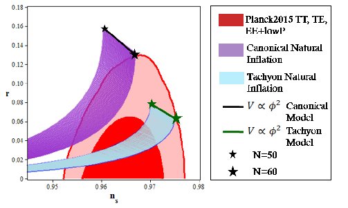
Figure 1: The tensor-to-scalar ratio versus the scalar spectral index in the background of the Planck2015 TT, TE, EE+lowP data.

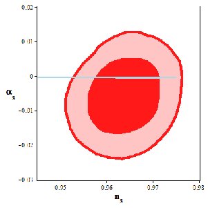
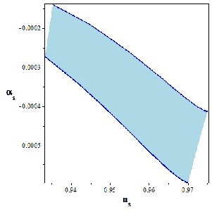
Figure 2: Running of the scalar spectral index versus the scalar spectral index in the background of the Planck2015 TT, TE, EE+lowP data. In the right panel we have zoomed out the cyan region of the left panel.

After obtaining these quantities, we can perform a numerical analysis on the model’s parameter space. To predict the values of $n_{s}$, $r$ and $\alpha_{s}$, we adopt $50\leq N\leq 60$. By plotting $r-n_{s}$ and $\alpha_{s}-n_{s}$ planes in the background of $68\%$ CL and $95\%$ CL regions of the Planck2015 TT, TE, EE+lowP data, we obtain some constraints on the parameter $\beta$. In figure 1 the region with violet color corresponds to the canonical Natural Inflation and the cyan region corresponds to our Tachyon Natural Inflation. We see that the Tachyon Natural Inflation is more consistent with observational data than the canonical Natural Inflation. The left panel of figure 2 shows the evolution of the running of the scalar spectral index with respect to the scalar spectral index in the background of the Planck2015 TT, TE, EE+lowP data. In the right panel of figure 2 we have zoomed out the cyan region of the left panel. Our analysis shows that for $N=50$, the parameters $n_{s}$, $\alpha_{s}$ and $r$ are consistent with the Planck2015 data if $f>\sqrt{\textbf{13}\lambda^{-1}}\,\Lambda^{-2}\,m_{pl}$. For $N=60$, these parameters are consistent with the Planck2015 data if $f>\sqrt{\textbf{12}\lambda^{-1}}\,\Lambda^{-2}\,m_{pl}$. We see that the bound on $f$ in TNI is in terms of $m_{pl}$, $\Lambda$ and $\lambda$ (contrary to the canonic NI in which the constraint on $f$ is only in terms of $m_{pl}$). Note that, if $\lambda\sim\Lambda^{-2}$, we get $\frac{f^{4}}{\Lambda^{4}}>(\sqrt{\textbf{13}}\,m_{pl})^{4}$ for $N=50$ and $\frac{f^{4}}{\Lambda^{4}}>(\sqrt{\textbf{12}}\,m_{pl})^{4}$ for $N=60$. In this respect, these constraints satisfy the condition (1). Table 1 gives a summary of constraints imposed on $f$ in our setup based on the observationally viable values of the scalar spectral index, running of the scalar spectral index and the tensor-to-scalar ratio for both $68\%$ and $95\%$ CL of the Planck2015 TT, TE, EE+lowP data. Table 2 is the same as table 1, but now by setting $\lambda\sim\Lambda^{-4}$ in order to state the obtained constraints just in terms of the reduced Planck mass.

Table 1: Constraints on $f$ based on the observationally viable values of the scalar spectral index, its running and the tensor-to-scalar ratio.

	$N=50$		$N=55$		$N=60$
$r-n_{s}\,,\,68\%$ CL	$\sqrt{\frac{18}{\lambda}}\frac{m_{pl}}{\Lambda^{2}}\leq f\leq\sqrt{\frac{90}{\lambda}}\frac{m_{pl}}{\Lambda^{2}}$		$\sqrt{\frac{15}{\lambda}}\frac{m_{pl}}{\Lambda^{2}}\leq f\leq\sqrt{\frac{65}{\lambda}}\frac{m_{pl}}{\Lambda^{2}}$		$\sqrt{\frac{14}{\lambda}}\frac{m_{pl}}{\Lambda^{2}}\leq f\leq\sqrt{\frac{40}{\lambda}}\frac{m_{pl}}{\Lambda^{2}}$
$r-n_{s}\,,\,95\%$ CL	$\sqrt{\frac{13}{\lambda}}\frac{m_{pl}}{\Lambda^{2}}\leq f$		$\sqrt{\frac{12.5}{\lambda}}\frac{m_{pl}}{\Lambda^{2}}<f$		$\sqrt{\frac{12}{\lambda}}\frac{m_{pl}}{\Lambda^{2}}\leq f$
$\alpha_{s}-n_{s}\,,\,68\%$ CL	$\sqrt{\frac{17}{\lambda}}\frac{m_{pl}}{\Lambda^{2}}\leq f$		$\sqrt{\frac{15}{\lambda}}\frac{m_{pl}}{\Lambda^{2}}\leq f\leq\sqrt{\frac{75}{\lambda}}\frac{m_{pl}}{\Lambda^{2}}$		$\sqrt{\frac{14}{\lambda}}\frac{m_{pl}}{\Lambda^{2}}\leq f\leq\sqrt{\frac{45}{\lambda}}\frac{m_{pl}}{\Lambda^{2}}$
$\alpha_{s}-n_{s}\,,\,95\%$ CL	$\sqrt{\frac{13}{\lambda}}\frac{m_{pl}}{\Lambda^{2}}\leq f$		$\sqrt{\frac{12.5}{\lambda}}\frac{m_{pl}}{\Lambda^{2}}<f$		$\sqrt{\frac{12}{\lambda}}\frac{m_{pl}}{\Lambda^{2}}\leq f$

Table 2: Constraints on $f$ based on the observationally viable values of the scalar spectral index, its running and the tensor-to-scalar ratio by adopting $\lambda=\Lambda^{-4}$.

	$N=50$		$N=55$		$N=60$
$r-n_{s}\,,\,68\%$ CL	$\sqrt{18}\,m_{pl}\leq f\leq\sqrt{90}\,m_{pl}$		$\sqrt{15}\,m_{pl}\leq f\leq\sqrt{65}\,m_{pl}$		$\sqrt{14}\,m_{pl}\leq f\leq\sqrt{40}\,m_{pl}$
$r-n_{s}\,,\,95\%$ CL	$\sqrt{13}\,m_{pl}\leq f$		$\sqrt{12.5}\,m_{pl}<f$		$\sqrt{12}\,m_{pl}\leq f$
$\alpha_{s}-n_{s}\,,\,68\%$ CL	$\sqrt{17}\,m_{pl}\leq f$		$\sqrt{15}\,m_{pl}\leq f\leq\sqrt{75}\,m_{pl}$		$\sqrt{14}\,m_{pl}\leq f\leq\sqrt{45}\,m_{pl}$
$\alpha_{s}-n_{s}\,,\,95\%$ CL	$\sqrt{13}\,m_{pl}\leq f$		$\sqrt{12.5}\,m_{pl}<f$		$\sqrt{12}\,m_{pl}\leq f$

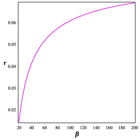
Figure 3: Tensor-to-scalar ratio versus the parameter $\beta$, for $\delta_{ns}=0.032$.

We can also find a constraint on the tensor-to-scalar ratio in terms of the scalar spectral tilt, $\delta_{ns}=1-n_{s}$. By solving equation (32) for ${\cal{G}}$, we find

$${\cal{G}}=-\frac{1+2\beta\delta_{ns}-\sqrt{1+6\beta\,\delta_{ns}}}{\beta\,\delta_{ns}}\,,$$ (35)

where the minus sign has been chosen due to the condition $-2\leq{\cal{G}}\leq 0$, which leads to the requirement $\beta>\frac{1}{2\delta_{ns}}$ or $f\geq\sqrt{\frac{1}{2\lambda\delta_{ns}}}\frac{m_{pl}}{\Lambda^{2}}$. With $n_{s}=0.968$, resulting in $\delta_{ns}=0.032$, the requirement $\beta\geq\frac{1}{2\delta_{ns}}$ demands the constraint $\beta\geq 15.6$ or $f\geq\sqrt{\frac{15.6}{\lambda}}\frac{m_{pl}}{\Lambda^{2}}$. Inserting expression (35) into equation (33) gives

$$r=8\,\delta_{ns}\,\frac{1+2\beta\delta_{ns}-\sqrt{1+6\beta\,\delta_{ns}}}{\left(1-\sqrt{1+6\beta\,\delta_{ns}}\right)^{2}}\,.$$ (36)

In figure 3 we have plotted the tensor-to-scalar ratio versus the parameter $\beta$, for $\delta_{ns}=0.032$. As figure shows, $r$ is an increasing function of $\beta$, with

$$\lim_{\beta\rightarrow\infty}r=\frac{8}{3}\,\delta_{ns}\,.$$ (37)

Therefore, a prediction of this model is $r\leq\frac{8}{3}\,\delta_{ns}$. This prediction becomes $r\leq 0.085$ for $\delta_{ns}=0.032$.

3 Reheating

One important stage in inflation models is the reheating at the end of inflation. It is necessary to warm up the universe sufficiently for subsequent processes. In this regard, we study this process in our TNI model and obtain some more constraints on the model’s parameter space. From the strategy used in Refs. [54, 55, 56, 57, 58], we can express the reheating parameters $N_{rh}$ and $T_{rh}$ in terms of the scalar spectral index in the TNI model. The relation between the number of e-folds and the scale factor at the horizon crossing ($a_{hc}$) as well as the scale factor at the end of inflation ($a_{end}$) is given by

$$N=\ln\left(\frac{a_{end}}{a_{hc}}\right)\,.$$ (38)

By introducing $\omega_{eff}$ as the effective equation of state parameter of the dominant component of the cosmic energy during the reheating epoch, we have $\rho\sim a^{-3(1+\omega_{eff})}$ for the energy density. Now, by using the scale factors at the end of inflation and the reheating era, we can write the number of e-folds during the reheating in terms of the energy density and the effective equation of state parameter in this era as follows

$$N_{rh}=\ln\left(\frac{a_{rh}}{a_{end}}\right)=-\frac{1}{3(1+\omega_{eff})}\ln\left(\frac{\rho_{rh}}{\rho_{end}}\right)\,.$$ (39)

By assuming $k_{hc}$ to be the value of $k$ at the horizon crossing and $a_{0}$ as the current value of the scale factor, we get

$$0=\ln\left(\frac{k_{hc}}{a_{hc}H_{hc}}\right)=\ln\left(\frac{a_{end}}{a_{hc}}\frac{a_{rh}}{a_{end}}\frac{a_{0}}{a_{rh}}\frac{k_{hc}}{a_{0}H_{hc}}\right)\,.$$ (40)

The following expression is obtained from equations (38), (39) and (40)

$$N+N_{rh}+\ln\left(\frac{k_{hc}}{a_{0}H_{hc}}\right)+\ln\left(\frac{a_{0}}{a_{rh}}\right)=0\,.$$ (41)

We can express the term $\frac{a_{0}}{a_{rh}}$ in terms of the temperature and energy density in the reheating era. To this end, we use the relation between energy density and temperature in reheating era as [56, 58]

$$\rho_{rh}=\frac{\pi^{2}g_{rh}}{30}T_{rh}^{4}\,,$$ (42)

with $g_{rh}$ to be the effective number of the relativistic species at the reheating era. Also, we can relate the scale factor at the reheating era to the temperature in this era by using the following equation [56, 58]

$$\frac{a_{0}}{a_{rh}}=\left(\frac{43}{11g_{rh}}\right)^{-\frac{1}{3}}\frac{T_{rh}}{T_{0}}\,.$$ (43)

In this relation the current temperature of the Universe is shown by $T_{0}$. By using equation (42) and (43) we find

$$\frac{a_{0}}{a_{rh}}=\left(\frac{43}{11g_{rh}}\right)^{-\frac{1}{3}}T_{0}^{-1}\left(\frac{\pi^{2}g_{rh}}{30\rho_{rh}}\right)^{-\frac{1}{4}}\,.$$ (44)

The energy density in our TNI model can be written in terms of the slow-roll parameter as

$$\rho=\frac{V}{\sqrt{1-\frac{2}{3\lambda}\epsilon}}\,.$$ (45)

Setting $\epsilon=1$ gives the energy density at the end of inflation phase as follows

$$\rho_{end}=\sqrt{\frac{3\lambda}{3\lambda-2}}\,V_{end}=\sqrt{\frac{3\lambda}{3\lambda-2}}\,\Lambda^{4}\Bigg{[}1+\cos\bigg{(}\frac{\phi_{end}}{f}\bigg{)}\Bigg{]}\,.$$ (46)

By using equations (39) and (46) we get

$$\rho_{rh}=\sqrt{\frac{3\lambda}{3\lambda-2}}\,V_{end}\exp\Big{[}-3N_{rh}(1+\omega_{eff})\Big{]}.$$ (47)

Now, by using equations (44) and (47) we can express $\frac{a_{0}}{a_{rh}}$ in terms of $N_{rh}$ and $\omega_{eff}$ as

$$\ln\left(\frac{a_{0}}{a_{rh}}\right)=-\frac{1}{3}\ln\left(\frac{43}{11g_{rh}}\right)-\frac{1}{4}\ln\left(\frac{\pi^{2}g_{rh}}{30\rho_{rh}}\right)-\ln T_{0}+\frac{1}{4}\ln\left(\sqrt{\frac{3\lambda}{3\lambda-2}}\,V_{end}\right)-\frac{3}{4}N_{rh}(1+\omega_{eff})\,.$$ (48)

From equations (15) (in order to obtain $H_{hc}$), (41) and (48), the e-folds number during reheating is obtained as

$$N_{rh}=\frac{4}{1-3\omega_{eff}}\Bigg{[}-N-\ln\Big{(}\frac{k_{hc}}{a_{0}T_{0}}\Big{)}-\frac{1}{4}\ln\Big{(}\frac{40}{\pi^{2}g_{rh}}\Big{)}-\frac{1}{3}\ln\Big{(}\frac{11g_{rh}}{43}\Big{)}+\frac{1}{2}\ln\Big{(}8\pi^{2}{\cal{A}}_{s}{\cal{W}}_{s}c_{s}^{3}\Big{)}$$

$$-\frac{1}{4}\ln\bigg{(}\sqrt{\frac{3\lambda}{3\lambda-2}}\,V_{end}\bigg{)}\Bigg{]}.\hskip 28.45274pt$$ (49)

Also from equations (39), (43) and (46) we find the temperature during reheating as follows

$$T_{rh}=\bigg{(}\frac{30}{\pi^{2}g_{rh}}\bigg{)}^{\frac{1}{4}}\,\bigg{[}\sqrt{\frac{3\lambda}{3\lambda-2}}\,V_{end}\bigg{]}^{\frac{1}{4}}\times\exp\bigg{[}-\frac{3}{4}N_{rh}(1+\omega_{eff})\bigg{]}\,.$$ (50)

To study the reheating phase numerically, it is useful to rewrite $N_{rh}$ and $T_{rh}$ in terms of the scalar spectral index. In this respect, from equations (30) and (35) we have

$$\cos\bigg{(}\frac{\phi_{hc}}{f}\bigg{)}=-{\frac{{\it n_{s}}\,\beta+\sqrt{-6\,{\it n_{s}}\,\beta+6\,\beta+1}-\beta-1}{\beta\left({\it n_{s}}-1\right)}}$$

$$=\frac{\sqrt{1+6\beta\delta_{ns}}-1}{\beta\delta_{ns}}-1\,.\hskip 76.82234pt$$ (51)

By using equations (28), (29) and (3) we can write the number of e-folds during inflation ($N$) in terms of $n_{s}$. In this way, we can obtain $N_{rh}$ and $T_{rh}$ as functions of the scalar spectral index in order to seek for numerical results. The results are shown in figures 4-7. Regarding to the bound on the scalar spectral index from Planck2015 data, in figure 4 we have plotted the ranges of $N_{rh}$ and $\omega_{eff}$ which makes the model observationally viable. In plotting the figures we have used the sample values of $\beta$ as $\beta=12$ (the left panel), $\beta=80$ (the middle panel) and $\beta=100$ (the right panel). These values of $\beta$ are chosen based on the constraints obtained in the previous section. Note also that we have used the amplitude of the scalar power spectrum as $A_{s}=2.196\times 10^{-9}$. In the reheating analysis also, we can obtain some constraints on $f$. This can be done by studying the $r-n_{s}$ plane for several ranges of the effective equation of state parameter during the reheating era and comparing the results with Planck2015 data. The situation has been demonstrated in figure 5. Since it is likely that the value of the effective equation of state parameter during the reheating phase to be in the range $0\leq\omega_{eff}\leq\frac{1}{3}$, we can obtain some further constraints on $f$ as well as the tensor-to-scalar ratio. Table 3 shows the constraints on $f$ and $r$. Our analysis shows that for $\omega_{eff}=0$ and $\omega_{eff}=\frac{1}{3}$ there is no upper limit on parameter $f$ (by considering the $95\%$ CL). Table 4 is the same as table 3, but now by setting $\lambda\sim\Lambda^{-4}$ in order to state the obtained constraints just in terms of the reduced Planck mass. Figure 6 shows the behavior of the number of e-folds during reheating versus the scalar spectral index in confrontation with Planck2015 data. To plot this figure we have adopted the sample values $\beta=12,\,20,\,80$ and $100$. Our analysis shows that for $20\leq\beta\leq 120$ the instantaneous reheating is favored by Planck2015 data. In figure 7 we have plotted the temperature during reheating versus the scalar spectral index for sample values of $\beta$ as have been adopted in figure 6. Based on the bounds on the scalar spectral index from Planck2015 data, we have obtained some constraints on $N_{rh}$ and $T_{rh}$ summarized in tables 5 and 6.

Table 3: Constraints on $f$ and $r$ based on the Planck2015 data and by considering the values of the effective equation of state parameter during the reheating era.

	$\omega_{eff}=0$		$\omega_{eff}=\frac{1}{6}$		$\omega_{eff}=\frac{1}{3}$		$\omega_{eff}=1$
$68\%$ CL	$---$		$\sqrt{\frac{16}{\lambda}}\frac{m_{pl}}{\Lambda^{2}}\leq f\leq\sqrt{\frac{80}{\lambda}}\frac{m_{pl}}{\Lambda^{2}}$		$\sqrt{\frac{13}{\lambda}}\frac{m_{pl}}{\Lambda^{2}}\leq f\leq\sqrt{\frac{30}{\lambda}}\frac{m_{pl}}{\Lambda^{2}}$		$\sqrt{\frac{11}{\lambda}}\frac{m_{pl}}{\Lambda^{2}}<f\leq\sqrt{\frac{18}{\lambda}}\frac{m_{pl}}{\Lambda^{2}}$
$95\%$ CL	$\sqrt{\frac{18}{\lambda}}\frac{m_{pl}}{\Lambda^{2}}\leq f$		$\sqrt{\frac{12}{\lambda}}\frac{m_{pl}}{\Lambda^{2}}<f$		$\sqrt{\frac{11}{\lambda}}\frac{m_{pl}}{\Lambda^{2}}<f\leq\sqrt{\frac{100}{\lambda}}\frac{m_{pl}}{\Lambda^{2}}$		$\sqrt{\frac{10}{\lambda}}\frac{m_{pl}}{\Lambda^{2}}<f<\sqrt{\frac{24}{\lambda}}\frac{m_{pl}}{\Lambda^{2}}$
$68\%$ CL	$---$		$0.024\leq r\leq 0.052$		$0.01\leq r\leq 0.027$		$0.0008\leq r\leq 0.001$
$95\%$ CL	$0.039\leq r\leq 0.092$		$0.019\leq r\leq 0.075$		$0.008\leq r\leq 0.058$		$0.0001\leq r\leq 0.002$

Table 4: Constraints on $f$ based on the Planck2015 data by adopting $\lambda=\Lambda^{-4}$.

	$\omega_{eff}=0$		$\omega_{eff}=\frac{1}{6}$		$\omega_{eff}=\frac{1}{3}$		$\omega_{eff}=1$
$68\%$ CL	$---$		$\sqrt{16}\,m_{pl}\leq f\leq\sqrt{80}\,m_{pl}$		$\sqrt{13}\,m_{pl}\leq f\leq\sqrt{30}\,m_{pl}$		$\sqrt{11}\,m_{pl}<f\leq\sqrt{18}\,m_{pl}$
$95\%$ CL	$\sqrt{18}\,m_{pl}\leq f$		$\sqrt{12}\,m_{pl}\leq f$		$\sqrt{11}\,m_{pl}<f\leq\sqrt{100}\,m_{pl}$		$\sqrt{10}\,m_{pl}<f<\sqrt{24}\,m_{pl}$

Figure 4: Observationally viable ranges of the parameters $N_{rh}$ and $\omega_{eff}$ in our TNI model based on the bounds on the scalar spectral index from Planck2015 data. The panels are corresponding to $\beta=12$ (left panel) $\beta=80$ (middle panel) and $\beta=100$ (right panel).

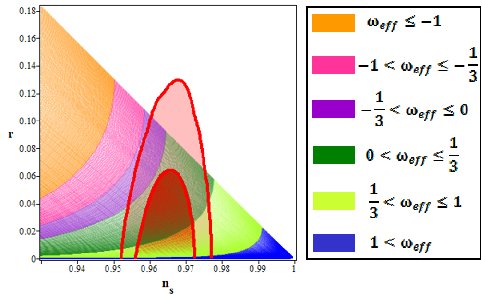
Figure 5: $r-n_{s}$ plane in TNI model for several ranges of the effective equation of state parameter during the reheating era in confrontation with Planck2015 TT, TE, EE+lowP data.

Table 5: The ranges of the number of e-folds parameter at reheating epoch in TNI model which are consistent with observational data.

	$f=\sqrt{\frac{12}{\lambda}}\frac{m_{pl}}{\Lambda^{2}}$		$f=\sqrt{\frac{20}{\lambda}}\frac{m_{pl}}{\Lambda^{2}}$		$f=\sqrt{\frac{80}{\lambda}}\frac{m_{pl}}{\Lambda^{2}}$		$f=\sqrt{\frac{100}{\lambda}}\frac{m_{pl}}{\Lambda^{2}}$
$\omega=-1$	$---$		$N_{rh}\leq 0.19$		$N_{rh}\leq 4$		$N_{rh}\leq 7$
$\omega=-\frac{1}{3}$	$---$		$N_{rh}\leq 0.32$		$N_{rh}\leq 10$		$N_{rh}\leq 14$
$\omega=0$	$---$		$N_{rh}\leq 0.61$		$N_{rh}\leq 19$		$N_{rh}\leq 28$
$\omega=1$	$---$		$N_{rh}\leq 69$		$N_{rh}\leq 18$		$N_{rh}\leq 10$

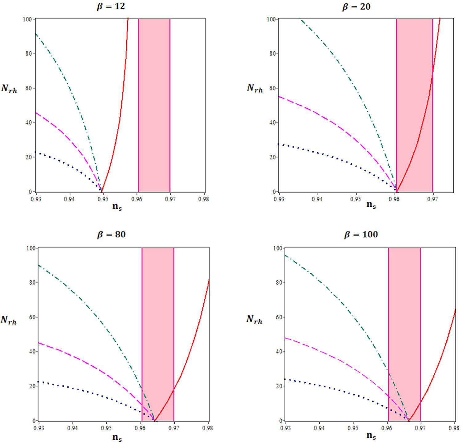
Figure 6: $N_{rh}$ versus $n_{s}$ for some sample values of $\beta$ in confrontation with Planck2015 data. The values of the effective equation of state parameter are chosen as $\omega_{eff}=-1$ (dotted line), $\omega_{eff}=-\frac{1}{3}$ (dashed line), $\omega_{eff}=0$ (dashed-dotted line) and $\omega_{eff}=1$ (solid line). The pink region is the bound on $n_{s}$ from Planck2015.

Figure 7: $\log_{10}\left(\frac{T_{rh}}{GeV}\right)$ versus $n_{s}$ for some sample values of $\beta$ and $\omega_{eff}$ in confrontation with Planck2015 data. The values of the effective equation of state parameter are chosen as $\omega_{eff}=-1$ (dotted line), $\omega_{eff}=-\frac{1}{3}$ (dashed line), $\omega_{eff}=0$ (dashed-dotted line) and $\omega_{eff}=1$ (solid line). The light blue region demonstrates the temperatures below the Electroweak scale, $T<100$ GeV, and the dark blue region shows the temperatures below the Big Bang Nucleosynthesis scale, $T<10$ MeV.

Table 6: The ranges of the temperature at reheating epoch in our TNI model which are consistent with observational data.

	$f=\sqrt{\frac{12}{\lambda}}\frac{m_{pl}}{\Lambda^{2}}$		$f=\sqrt{\frac{20}{\lambda}}\frac{m_{pl}}{\Lambda^{2}}$		$f=\sqrt{\frac{80}{\lambda}}\frac{m_{pl}}{\Lambda^{2}}$		$f=\sqrt{\frac{100}{\lambda}}\frac{m_{pl}}{\Lambda^{2}}$
$\omega=-\frac{1}{3}$	$---$		$\log_{10}\left(\frac{T_{rh}}{GeV}\right)\geq 14.9$		$\log_{10}\left(\frac{T_{rh}}{GeV}\right)\geq 9.5$		$\log_{10}\left(\frac{T_{rh}}{GeV}\right)\leq 6.82$
$\omega=0$	$---$		$\log_{10}\left(\frac{T_{rh}}{GeV}\right)\geq 14.5$		$\log_{10}\left(\frac{T_{rh}}{GeV}\right)\geq-1.3$		$---$
$\omega=1$	$---$		$---$		$---$		$---$

4 Summary

By considering a tachyon field to be responsible for Natural Inflation, we have constructed a Tachyon Natural Inflation. Tachyon Natural Inflation with large values of parameter $f$ (the width of the potential) meets the tachyon model with $\phi^{2}$ potential which is consistent with Planck2015 observational data. We have studied the cosmic inflation and linear perturbations in this setup. In this way, we have obtained the slow-roll parameters ($\epsilon$, $\eta$ and $\zeta$) and the main perturbation parameters such as the scalar spectral index, its running and the tensor-to-scalar ratio. Because of the form of the Lagrangian in this setup, these parameters have been obtained in terms of the height of potential ($2\Lambda^{4}$), its width ($f$), reduced Planck mass ($m_{pl}$) and the warp factor ($\lambda$). As we know, in canonical Natural Inflation (NI) these are obtained in terms of only the width of the potential and the reduced Planck mass. We have performed a numerical analysis on the model parameter space and compared the results with $68\%$ CL and $95\%$ CL regions of Planck2015 data. In this regard and by studying $r-n_{s}$ and $\alpha_{s}-n_{s}$ planes we have obtained some constraints on parameter $f$, which is in terms of $\lambda$, $\Lambda$ and $m_{pl}$. We have performed our analysis by adopting $N=50$, $N=55$ and $N=60$. By analyzing the perturbation parameters we have found lower limits on $f$, however there is no upper limits on this parameter in confrontation with $95\%$ CL of Planck2015 data. Note that, if we consider $\lambda\sim\Lambda^{-2}$, the obtained constraints satisfy the condition (1). As figure 1 shows, our TNI model has very good agreement with Planck2015 data, much better than the canonical natural inflation. We have also shown that a prediction of this model is $r\leq\frac{8}{3}\,\delta_{ns}$, where $\delta_{ns}$ is the scalar spectral tilt. Considering that from the Planck2015 data we have $\delta_{ns}=0.032$, we get the constraint $r\leq 0.085$. The reheating era after inflation has been studied also in this NTI model. We have obtained the number of e-folds and temperature during reheating era in terms of $n_{s}$, $\beta$ and $\omega_{eff}$. Taking into account that it is likely for the value of the effective equation of state parameter to be between $0$ and $\frac{1}{3}$, we have obtained some explicit constraints on the width of potential and the tensor-to-scalar ratio in this setup. These constraints are obtained based on the observationally viable values of the scalar spectral index from $68\%$ CL and $95\%$ CL regions of Planck2015 data. We have also studied the number of e-folds and temperature during the reheating era numerically. Regarding the bounds on the scalar spectral index from Planck2015 data set, we have obtained new constraints on $N_{rh}$ and $T_{rh}$.

In summary, the Tachyon Natural Inflation model presented in this paper is a cosmologically viable model (much better than the standard canonical natural inflation) which its perturbation parameters values lie well within the $95\%$ (and $68\%$) CL region of the Planck2015 dataset, even in large $f$ limit. Also, the effective equation of state parameter in this model for $0\leq\omega_{eff}\leq\frac{1}{3}$ gives the observationally viable values of the scalar spectral index and tensor-to-scalar ratio.

Acknowledgement
The work of K. Nozari has been supported financially by Research Institute for Astronomy and Astrophysics of Maragha (RIAAM) under research project number 1/5237-10.

References

- [1] A. Guth, Phys. Rev. D 23, 347 (1981).
- [2] A. D. Linde, Phys. Lett. B 108, 389 (1982).
- [3] A. Albrecht and P. Steinhard, Phys. Rev. D 48, 1220 (1982).
- [4] A. D. Linde, Particle Physics and Inflationary Cosmology (Harwood Academic Publishers, Chur, Switzerland, 1990). [arXiv:hep-th/0503203].
- [5] A. Liddle and D. Lyth, Cosmological Inflation and Large-Scale Structure, (Cambridge University Press, 2000).
- [6] J. E. Lidsey et al., Rev. Mod. Phys. 69, 373 (1997).
- [7] A. Riotto, [arXiv:hep-ph/0210162].
- [8] D. H. Lyth and A. R. Liddle, The Primordial Density Perturbation (Cambridge University Press, 2009).
- [9] J. M. Maldacena, JHEP 0305, 013 (2003).
- [10] F. C. Adams, K. Freese and A. H. Guth, Phys. Rev. D 43, 965 (1991).
- [11] K. Freese, J. A. Frieman and A. V. Olinto, Phys. Rev. Lett. 65, 3233 (1990).
- [12] K. Freese and W. H. Kinney, Phys. Rev. D 70, 083512 (2004).
- [13] K. Freese and W. H. Kinney, JCAP 1503, 044 (2015).
- [14] F. Adams, J. R. Bond, K. Frees, J, Frieman and Angela Olinto. Phys. Rev. D 47, 426 (1993).
- [15] K. Freese, [arXiv:astro-ph/9310012v1].
- [16] J. L. Cook, E. Dimastrogiovanni, D. Easson and L. M. Krauss, JCAP 04, 047 (2015).
- [17] G. German, A. Herrera-Aguilar, J. C. Hidalgo, R. A. Sussman and J. Tapia, [arXiv:1707.00957].
- [18] G. Ross and G. German, Phys. Lett. B 684, 199 (2010).
- [19] L. Visinelli, J. Cosmol. Astropart. Phys. 1109, 013 (2011).
- [20] H. Mishra, S. Mohanty and A. Nautiyal, [arXiv:1106.3039].
- [21] P. A. R. Ade et al., AA 594, A20 (2016).
- [22] P. A. R. Ade et al., AA 594, A13 (2016).
- [23] A. Sen, J. High Energy Phys. 10, 008 (1999).
- [24] A. Sen, J. High Energy Phys. 07, 065 (2002).
- [25] A. Sen, Mod. Phys. Lett. A 17, 1797 (2002).
- [26] G. W. Gibbons, Phys. Lett. B 537, 1 (2002).
- [27] T. Padmanabhan, Phys. Rev. D 66, 021301 (2002).
- [28] V. Gorini, A. Y. Kamenshchik, U. Moschella and V. Pasquier, Phys. Rev. D 69, 123512 (2004).
- [29] E. J. Copeland, M. R. Garousi, M. Sami and S. Tsujikawa, Phys. Rev. D 71, 043003 (2005).
- [30] M. Sami, P. Chingangbam and T. Qureshi, Phys. Rev. D 66, 043530 (2002).
- [31] A. Feinstein, Phys. Rev. D 66, 063511 (2002).
- [32] K. Nozari and N. Rashidi, Phys. Rev. D 88, 023519 (2013).
- [33] K. Nozari and N. Rashidi, Phys. Rev. D 90, 043522 (2014).
- [34] D. Kutasov [arXiv:hep-th/0408073].
- [35] S. Thomas and J. Ward, JHEP 0502, 015 (2005).
- [36] S. Thomas and J. Ward, JHEP 0510, 098 (2005).
- [37] S. Thomas and J. Ward, Phys. Rev. D 72 083519, (2005).
- [38] L Kofman and A. Linde, JHEP 0207, 004 (2002).
- [39] A. Frolov, L. Kofman and A. Starobinsky, Phys. Lett. B 545, 8 (2002).
- [40] X. Chen, Phys. Rev. D 72, 123518 (2005).
- [41] L. F. Abbott, E. Farhi and M. B. Wise, Phys. Lett. B 117, 29 (1982).
- [42] A. D. Dolgov and A. D. Linde, Phys. Lett. B 116, 329 (1982).
- [43] A. J. Albrecht, P. J. Steinhardt, M. S. Turner and F. Wilczek, Phys. Rev. Lett. 48, 1437 (1982).
- [44] B. R. Greene, T. Prokopec and T. G. Roos, Phys. Rev. D 56, 6484 (1997).
- [45] N. Shuhmaher and R. Brandenberger, Phys. Rev. D 73, 043519 (2006).
- [46] J. F. Dufaux, G. N. Felder, L. Kofman, M. Peloso and D. Podolsky, JCAP 0607, 006 (2006).
- [47] A. A. Abolhasani, H. Firouzjahi and M. Sheikh-Jabbari, Phys. Rev. D 81, 043524 (2010).
- [48] G. N. Felder, J. Garcia-Bellido, P. B. Greene, L. Kofman and A. D. Linde, Phys. Rev. Lett. 87, 011601 (2001) .
- [49] G. N. Felder, L. Kofman and A. D. Linde, Phys. Rev. D 64, 123517 (2001).
- [50] G. N. Felder, L. Kofman and A. D. Linde, Phys. Rev. D 59, 123523 (1999).
- [51] L. Kofman, A. D. Linde and A. A. Starobinsky, Phys. Rev. Lett. 73, 3195 (1994) .
- [52] J. H. Traschen and R. H. Brandenberger, Phys. Rev. D 42, 2491 (1990).
- [53] L. Kofman, A. D. Linde and A. A. Starobinsky, Phys. Rev. D 56 3258 (1997).
- [54] L. Dai, M. Kamionkowski and J. Wang, Phys. Rev. Lett. 113, 041302 (2014).
- [55] J. B. Munoz and M. Kamionkowski, Phys. Rev. D 91, 043521 (2015).
- [56] J. L. Cook, E. Dimastrogiovanni, D. Easson and L. M. Krauss, JCAP 04, 047 (2015).
- [57] R. -G. Cai, Z. -K. Guo and S. -J. Wang, Phys. Rev. D 92, 063506 (2015).
- [58] Y. Ueno and K. Yamamoto, Phys. Rev. D 93, 083524 (2016).
- [59] K. Nozari and N. Rashidi, Phys. Rev. D 95, 123518 (2017).
- [60] M. A. Amin, M. P. Hertzberg, D. I. Kaiser and J. Karouby , Int. J. Mod. Phys. D 24, 1530003 (2015).
- [61] V. F. Mukhanov, H. A. Feldman and R. H. Brandenberger, Physics Reports 215, 203 (1992).
- [62] D. Baumann, [arXiv:0907.5424][hep-th].
- [63] J. Bardeen, Phys. Rev. D 22, 1882 (1980).
- [64] A. De Felice and S. Tsujikawa, Phys. Rev. D 84, 083504 (2011).
- [65] A. De Felice and S. Tsujikawa, JCAP 1104, 029 (2011).
- [66] C. Cheung, P. Creminelli, A. L. Fitzpatrick, J. Kaplan and L. Senatore, JHEP 0803, 014 (2008).
- [67] G. Simard, D. Hanson, and G. Holder, ApJ 807, 166 (2015).
- [68] L. Boyle, K. M. Smith, C. Dvorkin and N. Turok, Phys. Rev. D 92, 043504 (2015).
- [69] Ø. Grøn, Universe 4, 15 (2018).