Spatially associated clump populations in Rosette from CO and dust maps

Abstract

Spatial association of clumps from different tracers turns out to be a valuable tool to determine the physical properties of molecular clouds. It provides a reliable estimate for the $X$-factors, serves to trace the density of clumps seen in column densities only and allows to measure the velocity dispersion of clumps identified in dust emission. We study the spatial association between clump populations, extracted by use of the Gaussclumps technique from ¹²CO ($1-0$), ¹³CO ($1-0$) line maps and Herschel dust-emission maps of the star-forming region Rosette, and analyse their physical properties. All CO clumps that overlap with another CO or dust counterpart are found to be gravitationally bound and located in the massive star-forming filaments of the molecular cloud. They obey a single mass-size relation $M_{\rm cl}\propto R_{\rm cl}^{\gamma}$ with $\gamma\simeq 3$ (implying constant mean density) and display virtually no velocity-size relation. We interpret their population as low-density structures formed through compression by converging flows and still not evolved under the influence of self-gravity. The high-mass parts of their clump mass functions are fitted by a power law ${\rm d}N_{\rm cl}/{\rm d}\,\log M_{\rm cl}\propto M_{\rm cl}^{\Gamma}$ and display a nearly Salpeter slope $\Gamma\sim-1.3$. On the other hand, clumps extracted from the dust-emission map exhibit a shallower mass-size relation with $\gamma=2.5$ and mass functions with very steep slopes $\Gamma\sim-2.3$ even if associated with CO clumps. They trace density peaks of the associated CO clumps at scales of a few tenths of pc where no single density scaling law should be expected.

1 Introduction

Observations of star-forming (SF) regions reveal the complex structure of the associated molecular clouds (MCs). The latter have been originally resolved into clumps of sub-parsec size. Recent high-resolution observations (e.g. with Herschel) show that the dense gas in MCs is predominantly concentrated in filamentary networks which probably play a central role in the star-formation process through further subfragmentation into dense prestellar cores with sizes below $0.1$ pc and densities up to $10^{6}$ cm^-3(André et al., 2014). A number of clump extraction techniques have been developed in the last three decades. They have been applied initially to molecular-line emission and dust-extinction maps and, later, to dust-emission maps which enabled in-depth studies of numerous SF regions in the Solar neighbourhood. As a major result, the obtained velocity-size and mass-size relationship for MC fragments and clumps emphasise the role of turbulence and gravity in the cloud evolution and their interplay (Larson, 1981; Solomon et al., 1987; Heyer & Brunt, 2004; Heyer et al., 2009). Virial analysis of clump populations hinted at possible mechanisms of clump formation (e.g. Myers & Goodman, 1988; Bertoldi & McKee, 1992; Dib et al., 2007). It also turned out that mass functions of dense clumps resemble the stellar initial mass function (Alves, Lombardi & Lada 2007; André et al. 2010; see, however, Clark, Klessen & Bonnell 2007). An open issue remains whether the extracted clumps represent real, distinct physical entities.

Clump-finding algorithms have been put to test with the advance of numerical simulations of MC evolution. Ballesteros-Paredes & MacLow (2002) and Shetty et al. (2010) investigated the role of projection effects on the clump properties and their virial analysis, while Beaumont et al. (2013) estimated the uncertainties of the derived characteristics of ¹³CO clumps. An important clue to link clump properties with the physics of star formation is provided through the derivation of a clump mass function (Stutzki & Güsten, 1990; Williams, Blitz & Stark, 1995; Kramer et al., 1998; Heithausen et al., 1998) and the interpretation of its parameters like slope and characteristic mass (e.g. Alves, Lombardi & Lada, 2007; Veltchev, Donkov & Klessen, 2013). Clump properties depend essentially on how the entire population is considered: as a set of independent entities or as a hierarchy in the position-position-position (PPP) / position-position-velocity (PPV) space. A widely used technique for non-hierarchical clump extraction is Clumpfind (Williams, de Geus & Blitz, 1994). It is based on eye inspection and identifies each peak on the intensity map with a clump. Recently Men’shchikov et al. (2012) proposed another non-hierarchical algorithm getsources which aims at 2D image decomposition in continuum maps at multiple scales and wavelengths and is appropriate for detection of clumps in crowded regions.

On the other hand, defining clumps as hierarchical objects reflects the fractal structure of MCs (Elmegreen & Falgarone, 1996; Elmegreen, 2002). This allows to link their properties to the general physics of SF regions as described by the above-mentioned scaling relations of mass and velocity. One hierarchical method for clump delineation is the Dendrogram technique (Rosolowsky et al., 2008) which traces the segmentation of cloud structures as one increases the threshold intensity.

Yet projection effects can be misleading in studies of cloud hierarchy. One can reduce them by the use of the clump-extraction technique Gaussclumps (Stutzki & Güsten, 1990; Kramer et al., 1998). It allows for a distinction of multiple coherent structures along the same line of sight by decomposing any structure into PPV or PPP Gaussian clumps which may overlap on the sky maps. For all smaller clumps in the resulting clump hierarchy the method derives significantly different properties from those that Clumpfind does (Schneider & Brooks, 2004). By allowing for the superposition of nested Gaussian clumps to form a large structure Gaussclumps also enables the retrieval of the hierarchical structure of a MC. Therefore, the approach of Gaussclumps is neither purely hierarchical, like the Dendrogram technique, nor purely non-hierarchical, like Clumpfind, but inherits advantages of both approaches. It characterises confined entities, but it also allows for the detection and analysis of nested structures from a single or multiple tracer(s). Our main goal in this work is to show what could be learned from spatial association of rich clump samples obtained via Gaussclumps on molecular-line (¹²CO, ¹³CO) and dust-emission maps.

The Rosette star-forming region is appropriate for this purpose – it has been intensively investigated in the last decades and mapped at different wavelengths with high angular resolution. Clumpy structures in the MC complex have been studied using various algorithms and tracers (Williams, Blitz & Stark, 1995; Schneider et al., 1998; Dent et al., 2009; Di Francesco et al., 2010). The statistical analysis of the highly filamentary structure of the complex and of the location of young stellar objects provides insight to the nature of the star-formation efficiency in individual clumps and it showed that the star formation in the cloud is not driven by radiative feedback (Schneider et al., 2012).

The paper is organised as follows. First, the used observational data are presented (Section 2). Section 3 reviews the algorithm and the calculation of clump sizes and masses. The adopted criterion for spatial association of clump populations and their statistics in Rosette is described in Section 4. Section 5 contains results from the performed physical analysis of the clump samples: size distributions and the relationships size vs. mass and mass vs. virial parameter. The clump mass functions are derived and studied in Section 6. Some problems and uncertainties are discussed in Section 7. A summary of this work is given in Section 8.

2 Observational data on Rosette MC

2.1 Selected region

In this study, we consider the Rosette molecular cloud (hereafter, RMC) with filamentary structures connected to it and traced on Herschel column-density maps (Motte et al., 2010; Hennemann et al., 2010; Di Francesco et al., 2010; Schneider et al., 2010, 2012), excluding the zone of direct interaction between the molecular cloud and the expanding H ii region around NGC 2244, the so called ‘Monoceros Ridge’ (Blitz & Thaddeus, 1980) (Fig. 1). The physical properties of the clump/core population in the Monoceros Ridge can be significantly influenced by the effects of stellar feedback such as gas compression by the expanding ionisation front or heating by the radiation from the OB cluster NGC 2244. Motte et al. (2010) detected more massive dense cores forming in this zone while Schneider et al. (2012) and Cambrésy et al. (2013) showed that there is no indication for large-scale triggering of star-formation further inside Rosette cloud.

Thus the region studied in this paper is restricted to zones where the star formation activity is probably not caused by direct external gas compression. A distance of $1330$ pc to the region was adopted (Lombardi, Alves & Lada, 2011) though distances up to $1.6$ kpc were also used in the literature (see Román-Zúñiga & Lada, 2008). The choice of distance value does not affect the analysis of scaling relations, the virial analysis and the derivation of the slopes of clump mass functions provided in the next sections.

2.2 Molecular-line and dust emission maps

We use maps of the Rosette star-forming region in ¹²CO $(J=1-0)$ (hereafter, ¹²CO) and ¹³CO $(J=1-0)$ (hereafter, ¹³CO) emission taken with the 14m telescope of Five College Radio Astronomy Observatory (FCRAO). These data sets were presented and discussed by Heyer, Williams & Brunt (2006). The beam FWHM of the CO data is $\sim$46″, the spectral resolutions are 0.127 km s^-1 (¹²CO) and 0.133 km s^-1 (¹³CO). All temperatures are given on the main beam brightness temperature scale.

The original maps of dust emission were obtained from Herschel observations at four wavelengths of PACS and SPIRE: 160, 250, 350 and 500 $\mu$m (see Schneider et al., 2010, 2012, for details). The maps were optimised for extended emission through the standard reduction methods in the HIPE pipeline and its scripts. For example, gains for extended emission are applied as applyExtendedEmissionGain was set to TRUE in the HIPE SPIRE pipeline. In addition, the Planck offsets for a zero-point correction were applied. The maps were convolved to a common angular resolution of 36″.

Contribution of the fore- or background in Rosette is not as significant as it is in other star-forming regions located close to or deep in the Galactic plane. Rosette is rather isolated which is also well reflected in velocity – only velocity structures in this region are detectable along the line of sight. In our view, possible overestimations of column density and, hence, of mass due to presence of fore- or background structures could hardly reach more than a few percent (in individual small subregions). Therefore we abstained from applying any fore- or background corrections to the Herschel maps. The major uncertainty of masses should be due to projection effects within the RMC, as specified in Sect. 5.1.

In a next step, a pixel-to-pixel grey-body fit to the data was performed, assuming that dust opacity per gas mass follows a power-law in the far infrared:

$$\kappa_{\nu}\,=\,0.1\,\Big{(}\frac{\nu}{1000~{}{\rm GHz}}\Big{)}^{b}~{}~{}\frac{{\rm cm}^{2}}{\rm g}~{},$$ (1)

with $b\equiv 2$ and leaving dust temperature and column density as free parameters. We assume here for dust emissivity the value for dense clouds used, e.g., by Hill et al. (2011), Russeil et al. (2013), Roy et al. (2013). It corresponds to a dust opacity of $2.3\times 10^{-25}\mathrm{cm}^{2}/$H at $\nu=1$ THz ($\lambda=300$ $\mu$m), when a mean mass $\mu_{\rm H,\,Gal}=1.37m_{\rm u}$ per hydrogen (with $m_{\rm u}$ as the atomic mass unit) is adopted. The various dust models from Ossenkopf & Henning (1994) cover opacities between $1.0\times 10^{-25}\mathrm{cm}^{2}/$H and $3.0\times 10^{-25}\mathrm{cm}^{2}/$H when assuming a gas-to-dust ratio of 100. The lower limit rather represents non-coagulated dust in diffuse clouds so that it is probably not representative for Rosette. For Planck cold cores Juvela et al. (2015) estimated $1.5\times 10^{-25}\mathrm{cm}^{2}/$H when converted to 300 $\mu$m. Taking this range, we estimate that the dust emissivity has an accuracy of $30-50$%. We also tested fits using lower exponents for the dust spectral index $1.5\leq\beta<2$, but found that the uncertainty in the resulting column density is smaller than the one governed by the absolute emissivity. Thus we estimate that the dust-based column-density map of Rosette has an accuracy of about $50$%, limited mainly by the uncertainty of the dust emissivity in the cloud and, to a lower degree, by the uncertainty in the SED-fitting procedure (constant line-of-sight temperature approximation).

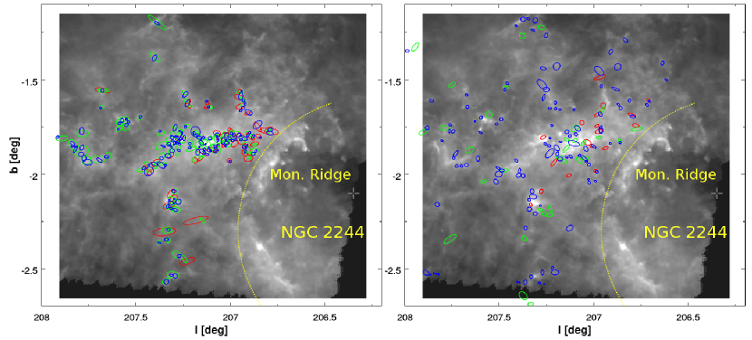
Figure 1: Locations of the extracted associated (left) and non-associated (right) clumps from ¹²CO (red), ¹³CO (green) and dust emission (blue), imposed on a Herschel map of Rosette (combined SPIRE 250 + 350 + 500 $\mu$m; available from the ESA Sky Archive http://sky.esa.int). The boundary of the region excluded from consideration is marked with dashed line (see text).

3 Clump extraction and characteristics

In this Section we comment on the adopted settings of the chosen clump-extraction technique and on the calculation of sizes and masses of clumps from molecular-line and dust emission maps.

3.1 Overview of the algorithm

The algorithm Gaussclumps was originally developed for the iterative decomposition of three-dimensional intensity distributions into individual clumps assuming a Gaussian shape (Stutzki & Güsten, 1990). However, it can be also applied to dust continuum maps (e.g. Motte, Schilke & Lis, 2003). Gaussclumps is implemented in two widely used software packages: Gildas and Cupid. We used the Gildas implementation for clump extraction on the ¹²CO and ¹³CO emission maps and the Cupid implementation for the Herschel data.

In both cases the choice of Gaussclumps control parameters is important. In general, when the three “stiffness” parameters are large ($s_{a}=s_{b}=s_{c}=50$), part of the noise peaks will be interpreted as clumps while adoption of very low values ($s_{a}=s_{b}=s_{c}=0.01$) excludes a significant fraction of the emission above the Gaussian noise from the clump composition procedure. We set $s_{a}=s_{b}=s_{c}=1.0$ following Kramer et al. (1998). The threshold below which the algorithm stops iterating is usually taken to be several times the data rms (Curtis & Richer, 2010; Pekruhl et al., 2013; Csengeri et al., 2014). We adopt a stringent threshold of 5 times the noise level for the input ¹²CO and ¹³CO maps. Dealing with the Herschel map, several test runs with different thresholds were made. A standard significance threshold of $3$ times the noise level yielded clumps with sizes $0.08~{}{\rm pc}\leq R_{\rm cl}\leq 0.47$ pc and masses $M_{\rm cl}$ between 2 and 268  $M_{\odot}$, whereas the mass range $M_{\rm cl}\lesssim 10$  $M_{\odot}$ was severely underpopulated. To increase the statistics of dense dust cores and the number of corresponding associations, we lowered the threshold stepwise. The best test value turned out to be $1.5\sigma$: the minimal $R_{\rm cl}$ shifted downwards just by $0.02$ pc, while many objects with characteristics of dense cores ($0.1\lesssim R_{\rm cl}/1~{}{\rm pc}\lesssim 0.3$, $M_{\rm cl}\leq 10$  $M_{\odot}$) appeared. Thus the total number of dust clumps increased by a factor of 2.5, while the number of associations (as defined in Sect. 4.1) increases by a factor of two. As the ¹²CO and ¹³CO clumps occupy only a small fraction of the map (see Fig. 1) this close correspondence indicates that most associated dust clumps are real. The adopted $1.5\sigma$ threshold limit to detect their peaks corresponds to a column density $N_{\rm lim}(\rm dust)=1.9\times 10^{21}$ cm^-2.

3.2 Sizes and masses of Gaussian clumps

The effective diameter of a Gaussian clump, extracted from a molecular-line emission map, is calculated as the geometrical mean of its major and minor axes on the sky plane (position-position space):

$$D_{\rm cl}=\sqrt{\Delta x_{\rm cl}\,\Delta y}_{\rm cl}~{}~{},$$

where $\Delta x_{\rm cl}$ and $\Delta y_{\rm cl}$ are defined as beam-deconvolved full widths of half-maxima (FWHM) of the fitted Gaussian curves along those directions, converted to linear sizes. Hereafter, we label ‘clump size’ the half of the effective diameter $R_{\rm cl}=0.5D_{\rm cl}$. Our observational data allow for linear resolutions are of $0.15$ pc (CO maps) and $0.12$ pc (dust maps), respectively.

The masses of the CO clumps were derived through three-dimensional integration of the brightness temperature $T_{\rm b}$ over the PPV space:

$$M_{\rm cl}{\rm(CO)}=\mu_{\rm mol}X\int\!\!\!\!\int\!\!\!\!\int T_{\rm b}\,dxdydv~{}~{}~{}~{}~{}~{}~{}~{}~{}~{}~{}~{}~{}~{}~{}~{}~{}~{}~{}~{}~{}~{}~{}~{}~{}~{}~{}~{}~{}~{}~{}~{}~{}~{}~{}~{}~{}~{}~{}~{}~{}~{}~{}$$

$$=\mu_{\rm mol}XT_{\rm b,\,0}\int\!\!\!\!\int\!\!\!\!\int e^{-\frac{(x-x_{0})^{2}}{2\sigma_{x}^{2}}}\!e^{-\frac{(y-y_{0})^{2}}{2\sigma_{y}^{2}}}\!e^{-\frac{(v-v_{0})^{2}}{2\sigma_{v}^{2}}}\,dxdydv$$

$$=\Big{(}\frac{1}{2}\sqrt{\frac{\pi}{\ln 2}}\Big{)}^{3}\mu_{\rm mol}XT_{\rm b,\,0}\,\Delta x_{\rm cl}\,\Delta y_{\rm cl}\,\Delta v_{\rm cl}~{}~{}~{}~{}~{}~{}~{}~{}~{}~{}~{}~{}~{}$$ (2)

where $T_{\rm b,\,0}$ is the peak value of $T_{\rm b}$ within the given clump, $(x_{0},y_{0},v_{0})$ are the positions of its centre in the PPV space, $\Delta v_{\rm cl}=2\sigma_{\rm cl}\sqrt{2\ln 2}$ is the FWHM in velocity and $\mu_{\rm mol}=2.74m_{\rm u}$ is the mean particle mass in molecular gas. The adopted estimates of the conversion factors $X$ from integrated CO (¹²CO or ¹³CO) intensity to hydrogen column density $N$ are discussed in Sect. 5.1.

Formula (2) was used by Stutzki & Güsten (1990) to derive masses of Gaussian clumps, extracted from maps of an optically thin tracer (C¹⁸O). Why it is applicable also to ¹²CO and ¹³CO clumps in the Rosette region? Optical depth of ¹³CO $(J=1-0)$ in various zones in RMC was assessed by (Schneider et al., 1998) as several intensity ratios have been modelled with external UV radiation. This line might be optically thick in the Monoceros ridge, at the position of the infrared source AFGL 961 and in the center zone $(l\sim 207.\!^{\circ}1,~{}b\sim-1.\!^{\circ}8)$, i.e. for a few positions, in the vicinity of very high column density peaks. The Monoceros ridge (cf. Fig. 1) and the clumps identified with AFGL 961 were excluded from our consideration whereas a few ones located in the centre zone would hardly affect the results presented in the next sections. For the remaining zones of lower (column) density gas, it can be assumed that ¹³CO line is predominantly optically thin. The latter was shown also by Williams, Blitz & Stark (1995) whose selected region in Rosette largely coincides with ours (see their Fig. 1).

In regard to the Gaussian clumps, extracted from maps of the optically thick ¹²CO $(1-0)$ emission, Kramer et al. (1998) found that their mass is still proportional to $XT_{\rm b,\,0}\,\Delta x_{\rm cl}\,\Delta y_{\rm cl}\,\Delta v_{\rm cl}$, “although the applicability of the $X$-factors from the literature to individual clumps may be questionable” (Sect. 3.2.2 therein). In this study we work with an averaged $X$-factor, derived from associations of ¹²CO/¹³CO clumps with dust counterparts (i.e. extracted from an optically thin emission, Sect. 5.1). Therefore the ¹²CO clump mass, calculated from equation (2) could be underestimated – in the worst case – by some constant factor. However, this would not affect neither the slopes of the studied scaling relations, nor the virial analysis since all ¹²CO clumps have been found to be gravitationally bound (Sect. 5.4.2).

The masses of the dust clumps, extracted from the Herschel map, were obtained in analogous way to equation (2), through two-dimensional integration of column density:

$$M_{\rm cl}{\rm(dust)}=\Big{(}\frac{1}{2}\sqrt{\frac{\pi}{\ln 2}}\Big{)}^{2}\mu_{\rm H,\,Gal}N_{0}\,\Delta x_{\rm cl}\,\Delta y_{\rm cl}~{}~{},$$ (3)

where $N_{0}$ is the peak value of column density within the clump and the adopted mean particle mass $\mu_{\rm H,\,Gal}=1.37m_{\rm u}$ is representative for Galactic abundances of atomic and molecular hydrogen and other elements (Draine, 2011).

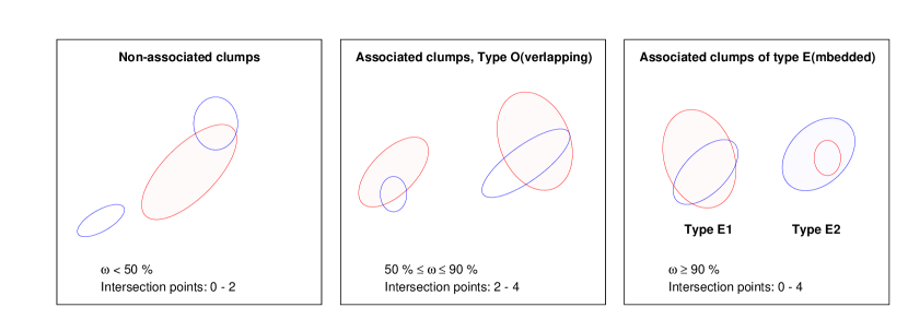
Figure 2: Criteria for association of Gaussian clumps from Population 1 (red) and Population 2 (blue), based on the value of the overlap coefficient $\omega$ (see text): non-associated (left), overlapping (middle) and embedded (right) clumps.

4 Spatial association between clump populations

Cross-identification (hereafter, association) of clumps from different tracers could be used as a tool to determine the physics of structures in MCs. In this Section we present a method to associate Gaussian clumps, introduce two types of associated clumps and provide statistics of the associated populations in the RMC.

4.1 Association between Gaussian clumps

Various tracers of cloud structure are sensitive to different ranges of density and optical depth. While the $J=1\rightarrow 0$ lines of ¹²CO and ¹³CO are typical tracers of molecular gas with densities $n\gtrsim 10^{2}$ cm^-3 and $n\gtrsim 10^{3}$ cm^-3, respectively, the far-infrared and submillimetre emission of dust enables one to trace the cloud structure from very low densities up to its dense cores ($n>10^{5}$ cm^-3). Therefore it is instructive to perform association between the extracted clump populations and to compare their locations and physical characteristics.

Since the projections of CO PPV clumps onto the celestial plane as well as the 2-dimensional clumps extracted from Herschel maps through Gaussclumps are ellipses, an appropriate criterion to associate clump pairs should be based on the theory of intersecting ellipses. We make use of a method developed by Hughes & Chraibi (2012). Its output are the number of intersection points and the intersection area of a considered pair of ellipses. In our treatment, the ellipse representing each clump is defined by the half-maximum contour.

The applied criterion for clump association is illustrated in Fig. 2. As one considers a pair of clumps from two samples, Population 1 and Population 2, the overlap coefficient $\omega$ is defined as the intersection area, normalised to the area of the smaller ellipse. In case of zero or one intersection points the ellipses do not overlap at all ($\omega=0$ %) or the smaller one is completely embedded into the larger ($\omega=100$ %). When the intersection points are 2, 3 or 4, the value of $\omega$ is decisive to discriminate between non-associated, overlapping and embedded clumps. To distinguish non-associated from overlapping clumps (Type O) we adopt a conservative range $50$%$\leq\omega<90$ %. Type E (embedded) is assigned to clump pairs with $\omega\geq 90$ %; such criterion is strong enough to ensure that most of the mass of a centrally condensed clump is contained in the overlap area. Two subclasses of type E are introduced depending on whether the clump from Population 1 is larger than its associate from Population 2 (Type E1), or vice versa (Type E2). An additional requirement for associating a ¹²CO and a ¹³CO clump is that the velocity ranges $(v_{0}-\Delta v_{\rm cl}/2)\leq v\leq(v_{0}+\Delta v_{\rm cl}/2)$ in both tracers contain at least one velocity channel in common.

Table 1: Statistics of the associated Gaussian clumps in RMC.

Tracer	Nr. of clumps
	In total	Associated
12CO	68	49
13CO	130	99
Dust	249	133

Table 2: Statistics of the associated pairs in RMC. The last two (one) columns contain the number ratios between the number of associations of different type.

Associated pairs			Number ratios
Pop 1-Pop 2	Nr.${}^{\ast}~{}$	Notation in Figs.	E1/O	E2/O
		3, 4, 7, 8, 9, 11
12CO - Dust	63	diamonds	0.80	0.03
13CO - Dust	112	squares	1.07	0.07
12CO - 13CO	37	circles	0.76	0.00
Associations with the same population
			E/O
12CO - 12CO	11	–	0.57
13CO - 13CO	12	–	0.20
Dust - Dust	7	–	1.33

$\ast$ Some clumps of Population 1 belong to more than one pair.

4.2 Associated clumps in Rosette

The associated objects populate the dense, main star-forming region in the RMC and its most pronounced filaments (Fig. 1, left; cf. Fig. 1 in Schneider et al. 2012). In contrast, the non-associated clumps are widely distributed over the cloud (Fig. 1, right); the few non-associated ¹²CO objects occur only at $l<207.\!\!^{\circ}3$. Most non-associated ¹³CO clumps are detected in channels of high radial velocity.

In Tables 1 and 2 we provide statistics of the associated clumps from each population. About 75 % of all CO clumps (¹²CO and ¹³CO) have at least one associate in one or both of the other tracers. Considering the dust clump population, the fraction of associated clumps is only 53 %. Twenty ¹²CO clumps in total have associates in the other two tracers; several of them are associated with more than one ¹³CO and/or dust clump. The vast majority of the non-associated dust clumps are small ($R_{\rm cl}<0.3$ pc), low mass ($M_{\rm cl}<10$ $M_{\odot}$) objects; part of them may be artefacts from our low detection limit.

Among the associated clump pairs (Table 2), Type O and Type E turn out to be equal or close in number. Considering only pairs of Type E, dust clumps are – in general – embedded into their CO counterparts and ¹³CO clumps are embedded into ¹²CO ones. The exceptions enable us to estimate the $X$-factors (Sect. 5.1). We also computed the associations for clumps of the same tracer to quantify hierarchies but the statistics of these associated pairs is poor due to the limited dynamic range of clump sizes. Their analysis provides reference values in the study of the mass-size relationship (cf. Sect 5.2).

5 Physical analysis

The analysis in this Section is focused on the associated clump populations. Since the calculated clump masses depend crucially on the $X$-factor (cf. Sect. 3.2), we suggest first an approach to estimate its average value in the RMC (Sect. 5.1). The derived size-mass relationships are presented in Sect. 5.2. In view of these and of the clump size distributions, we explore the strength of our method to associate individual clumps, investigating cross-correlations between the three maps of Rosette as functions of the spatial scale (Sect. 5.3). Then, in Sect. 5.4, we study the velocity dispersions of the clumps seen in ¹²CO and ¹³CO which enables the virial analysis of all clump populations.

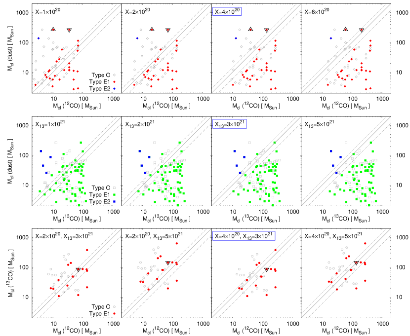
Figure 3: Comparison of clump masses from the associated pairs of Population 1 (absciss) and Population 2 (ordinate): ¹²CO-dust (top), ¹³CO-dust (middle) and ¹²CO- ¹³CO(bottom). The test values of the $X$-factors are given in units [cm^-2K^-1km^-1s]; the adopted ones are put in a box. The dashed lines on both sides of the identity line represent the adopted uncertainty of mass estimates (see text). The triangles mark the dust cores identified with AFGL 961 and PL3 that were excluded from the analysis.

5.1 Estimation of the X-factor

Masses of condensations delineated in molecular-line maps are usually derived from object’s intensity $W$ integrated over its area and line-of-sight through the factor $X=N(\mathrm{H}_{2})/W$. Our first task in the analysis of the extracted clumps is to achieve a highly plausible estimate of $X$ for the tracers ¹²CO and ¹³CO based on clump associations. We use the masses of dust clumps $M_{\rm cl}({\rm dust})$ as reference values for a comparison with the masses of their CO associates. The elaborated procedure of pixel-to-pixel determination of column density (Section 2.2) should yield $M_{\rm cl}({\rm dust})$ with uncertainties of better than 50 % (Roy et al., 2013).

Observational works on many nearby MCs indicate that the $X$-factor for ¹²CO (hereafter, just $X$) in the Galaxy is approximately constant (Dame, Hartmann & Thaddeus, 2001; Bolatto, Wolfire & Leroy, 2013). Theoretical models also show that a constant $X$ is justified, except in case of high metallicities (Szűcs, Glover & Klessen, 2016). The widely adopted reference value for the Milky Way is:

$$X_{\rm MW}(^{12}\mathrm{CO})\equiv X_{\rm MW}=2\times 10^{20}~{}\mathrm{cm}^{-2}\mathrm{K}^{-1}\mathrm{km}^{-1}\mathrm{s}$$ (4)

However, numerical simulations including details of the hydrogen, carbon, and oxygen chemistry indicate a significant variation of the $X$-factor ($1\lesssim X/X_{\rm MW}\lesssim 10^{4}$) in the low-extinction regime $A_{V}\lesssim 3.5$ (Glover & Mac Low, 2011; Shetty et al., 2011). Ossenkopf (2002) showed that $X$ might increase by two orders of magnitude from low- to high-density regimes due to optical depth effects. More than half of all associated ¹²CO clumps in the RMC populate regions where such variations of $X$ should be expected. Therefore, instead of choosing a priori some average value of $X$ in RMC, we estimate it by comparing the masses of gaseous and dust clumps from the embedded pairs (type E).

Our basic assumption is that, within the error bars, the mass of the embedded clump should be smaller than that of its counterpart in the other tracer: $M_{1}\geq M_{2}$ for pairs of Type E1 and $M_{1}\leq M_{2}$ for pairs of Type E2 (cf. Fig. 2). Per definition, associated pairs of both types are separated by the identity line in the size-size diagram (see Fig. 11 in the Appendix). Such a separation should also be observed in the mass-mass diagram if the Gaussian clumps in a pair are indeed spatially embedded.

Under this assumption, we varied $X/X_{\rm MW}$ between $0.1$ and $10$ and calculate the masses of ¹²CO clumps $M_{\rm cl}$ (¹²CO) for each test value. Then, by comparing $M_{\rm cl}$ (¹²CO) with $M_{\rm cl}$ (dust) of the embedded dust associates, one can probe the range of plausible values of $X$ (Fig. 3, top). Two pairs of clumps have to be excluded. The infrared sources AFGL 961 and PL3 (Phelps & Lada (1997), clump D in Poulton et al. 2008) show irregular ¹²CO line profiles indicating strong self-absorption and outflows (see Schneider et al., 1998) so that they hardly trace the column density structure. For completeness they are shown in Fig. 3 but were excluded from further consideration. For all other clumps we adopt a possible 40% uncertainty of the calculated masses of PPV clumps due to projection effects (Beaumont et al., 2013). Visual inspection of the mass-mass diagrams of the associated ¹²CO-dust pairs of type E1 (first row of Fig. 3) shows that within the error bars values of $X$ between $2\times 10^{20}~{}\mathrm{cm}^{-2}\mathrm{K}^{-1}\mathrm{km}^{-1}\mathrm{s}$ and $6\times 10^{20}~{}\mathrm{cm}^{-2}\mathrm{K}^{-1}\mathrm{km}^{-1}\mathrm{s}$ provide $M_{\rm cl}$(¹²CO)$>M_{\rm cl}$ (dust).

The possible values of $X(^{13}\mathrm{CO})$ (hereafter, $X_{13}$) are obtained in analogous way. We probed the test range $1\leq X_{13}/(8\times 10^{20}~{}\mathrm{cm}^{-2}\mathrm{K}^{-1}\mathrm{km}^{-1}\mathrm{s})\leq 10$; some mass-mass diagrams are shown in the central row of Fig. 3. The reference value corresponds to $N(\mathrm{H}_{2})/N(^{13}\mathrm{CO})=7\times 10^{5}$ (Frerking, Langer & Wilson, 1982), which is widely used in studies of large MC complexes (e.g. Nagahama et al., 1998; Zhang, Xu & Yang, 2014), combined with the LTE emissivity $W/N(^{13}\mathrm{CO})=9\times 10^{-16}$  K km s^-1 cm² at a temperature of $T=15$ K (Mangum & Shirley, 2015). The objects of Types E1 and E2 form clearly separable groups on the mass-mass diagram. This enables us to constrain $X_{13}$ in a narrow range between $3\times 10^{21}~{}\mathrm{cm}^{-2}\mathrm{K}^{-1}\mathrm{km}^{-1}\mathrm{s}$ and $5\times 10^{21}~{}\mathrm{cm}^{-2}\mathrm{K}^{-1}\mathrm{km}^{-1}\mathrm{s}$ consistent with studies where the ratio ${}^{12}{\rm C}/^{13}{\rm C}$ has been probed (e.g. Blake et al., 1987). Due to the occurrence of both subtypes of embedding this constraint is much stronger than for ¹²CO.

Finally we probe the associated clump pairs ¹³CO-¹²CO on the mass-mass diagrams using the limits on $X$ and $X_{13}$ factors obtained above (bottom row in Fig. 3). Here it becomes clear that the constraint that all ¹³CO clumps are embedded in ¹²CO clumps, consequently having masses $M_{\rm cl}$ (¹³CO)$\leq M_{\rm cl}$ (¹²CO), is only fulfilled if we use the combination of $X/X_{\rm MW}=2$ and $X_{13}=3\times 10^{21}~{}\mathrm{cm}^{-2}\mathrm{K}^{-1}\mathrm{km}^{-1}\mathrm{s}$. In this way, the concept of clump associations provides a very stringent limit on the $X$ and $X_{13}$ factors in the cloud if we assume that they are constant. The abovementioned estimates of $X/X_{\rm MW}$ and $X_{13}$ are taken as average values in the RMC to calculate clump masses.

5.2 Size-mass relationships

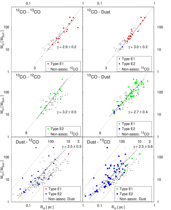
Figure 4: Size-mass diagrams of the clump populations. The symbols are the same as in Fig. 3 but note the interchange of Types E1 and E2 depending on clumps of which tracer are taken to be Population 1. Dots show the corresponding locations of non-associated clumps of each tracer. The derived scaling relations (solid; cf. Table 3, column 5) and lines of constant mean density $\langle n\rangle$ in units $10^{3}$ cm^-3(dashed) are indicated.

Table 3: Size-mass relationships for different clump populations.

Tracer	Total population	Associated population
	$\gamma$	Tracer	Clumps	$\gamma$
12CO	$2.5\pm{\scriptstyle 0.3}$	13CO	30	$2.9\pm{\scriptstyle 0.2}$
		Dust	40	$3.0\pm{\scriptstyle 0.2}$
		12CO	17	$3.0\pm{\scriptstyle 0.1}$
13CO	$2.6\pm{\scriptstyle 0.5}$	12CO	37	$3.2\pm{\scriptstyle 0.5}$
		Dust	80	$2.7\pm{\scriptstyle 0.4}$
		13CO	22	$2.9\pm{\scriptstyle 0.2}$
Dust	$2.3\pm{\scriptstyle 0.5}$	12CO	58	$2.5~{}{\scriptstyle\pm 0.5}$
		13CO	105	$2.5~{}{\scriptstyle\pm 0.6}$
		Dust	13	$2.7~{}{\scriptstyle\pm 0.7}$

The mass-size relationship $M\propto R^{\gamma}$ reflects the scaling of density in molecular clouds (Larson, 1981; Solomon et al., 1987; Heyer et al., 2009). Table 3 contains the mass scaling indices $\gamma$ obtained from the studied samples of Gaussian clumps in the RMC. The values for the full sample of clumps in each tracer (column 2) are about $\gamma=2.4$, consistent with other studies at scales below $1$ pc (e.g. Heithausen et al., 1998; Hennebelle & Falgarone, 2012).

However, tightening the scope of consideration only to the associated clump populations yields an increase of the scaling indices $\gamma$ by 0.3–0.5. From the table it becomes clear that the associated clumps do not describe exactly the same material because it makes a difference whether we study e.g. the properties of CO clumps that have a dust counterpart or the properties of these dust counterparts.

For the associated CO clumps (Fig. 4, top and middle, and Table 3, column 5) $\gamma\simeq 3$ within the uncertainties. In other words, these populations obey a relation of constant mean volume density $\langle n\rangle$ of the molecular gas in the range $3\times 10^{3}$ to $8\times 10^{3}$ cm^-3. The result is confirmed when associated clumps from a single tracer are considered (see ¹²CO-¹²CO and ¹³CO-¹³CO in Table 3). On the other hand, dust clumps with CO counterparts exhibit a shallower mass scaling that is only slightly higher than the one obtained from the full sample. Test runs of Gaussclumps on the dust column-density map showed that the result is independent of the chosen noise level.

5.3 Cross-correlation between the maps

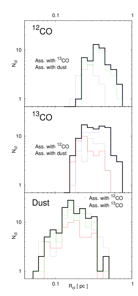
Figure 5: Distribution of clump sizes in the different populations. The solid lines show the distribution of associated clumps (black – all, color – with the specified tracer only), the dashed lines those of non-associated clumps.

The variation of the mass scaling index for associated clump populations prompt us to probe the strength of the association method. An appropriate way to do this is by study the cross-correlation between the maps in the corresponding tracers as a function of abstract spatial scale.

Comparing the size distributions of the associated and non-associated clumps in Figs. 4 and 5 one can see that the non-associated ¹²CO clumps tend to be smaller by about a factor of two than those associated with dust or ¹³CO. For ¹³CO clumps the trend also holds for associations with ¹²CO, but not for associations with dust. In contrast there is no size dependence for associations from the viewpoint of dust clumps. Moreover, the size range and distribution of the ¹²CO clumps and the ¹³CO clumps is similar while the dust clumps are on average much smaller. Using a naive comparison of the size distributions of associated and non-associated clumps, one expects a better correlation of ¹²CO with the other tracers when increasing the scale. In contrast, from the dust clump size spectrum one would not expect a scale dependence of the correlation between dust and other tracers. When straightforwardly comparing ¹²CO and dust, both assumptions are obviously mutually exclusive.

The mutual size relations between different tracers can be directly measured by investigation of the cross-correlations between the three different maps as a function of the spatial scale. To this aim, we use the wavelet-based weighted cross-correlation (WWCC) tool (Arshakian & Ossenkopf, 2016) that studies the degree of correlation of structures seen in a pair of maps as a function of the structure size. The method filters the two maps with a wavelet of a characteristic size so that only structures of that size remain visible and then computes the cross-correlation between the two filtered maps. In this way only structures of the same scale are compared. By using different wavelet sizes we obtain a spectrum of cross-correlation coefficients. Every point in the individual maps can be weighted by a noise weight to adjust the statistical significance of the result to the actual measurement uncertainties. In case of systematic shifts of characteristic structures between the two compared maps the WWCC can also measure their mutual displacement.

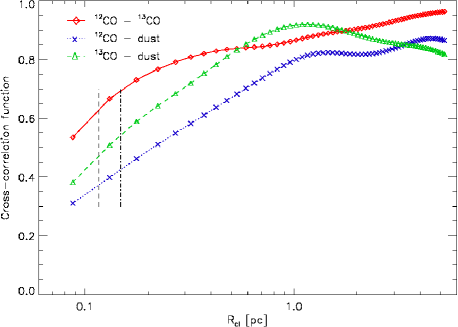
Figure 6: Spectra of wavelet-based cross-correlation coefficients as a function of the clump size scale for the three pairs of maps in the RMC. For a comparison to the clump size spectra, the wavelet scale $l$ has been divided by $8/\sqrt{8\ln(2)}\approx 3.4$ to obtain corresponding clump radius units, $R_{\rm cl}$. The two vertical dashed lines indicate the resolution limit of the observations of 36^′′ (dust) and 46^′′ (¹²CO,¹³CO).

Figure 6 shows the spectra of cross-correlation coefficients as a function of scale for all three pairs of maps of the RMC. The calibration of the wavelet spectrum for individual Gaussian clumps by Arshakian & Ossenkopf (2016) enables translation of the wavelet scale $l$ into the radius of the clumps: $l\approx 3.4R_{\rm cl}$. Thus the cross-correlation spectrum can be plotted in Fig. 6 directly on the clump radius scale and thus a direct comparison to Fig. 4 is possible. The spectra of the cross-correlation of ¹²CO with either of the other two maps show a monotonous increase towards larger scales. Individual small structures can significantly deviate between the different tracers, partially due to the noise impact at small scales, but towards larger scales all maps trace the same overall structure of the molecular cloud. For small and large clump sizes, the structures in both CO isotopologue maps show the best matches, providing the highest cross-correlation coefficient. At very large scales, the cross-correlation coefficient even approaches unity which suggests an extremely good match of the large-scale molecular distribution. In contrast, the cross-correlation with the dust shows a more complicated behaviour. The large dynamic range of the dust map traces both low-level extended material and small dense cores. The wide-spread low intensity emission also traced by ¹²CO hardly contributes to the clump extraction but dominates the cross-correlation function at large scales. Individual high-column-density clumps match the dense structures also traced by ¹³CO. On scales around 1 pc ¹³CO is even best correlated with the dust. Both species show the same prominent structures of that size. This indicates that for structure sizes around 1 pc the ¹³CO emission is a reasonable column density tracer, getting optically thicker at smaller scales so that it is suppressed relative to the dust below 1 pc and overamplified relative to the rest of the map at larger scales. Therefore, the correlation with dust drops again at large scales. ¹²CO is already optically thick at much larger scales. For that reason it shows a very extended emission and a good correlation with the wide-spread dust distribution at the large scales but a low correlation at small scales.

From the monotonously increasing cross-correlation between all maps at sizes below 1 pc we would expect to find more clump associations with increasing clump sizes. The effect of more ¹²CO associations with clump size is clearly visible in Figs. 4 and 5. At large $R_{\rm cl}>0.4$ pc even all ¹²CO clumps are associated, suggesting a more perfect match than the cross-correlation shows. However, looking from the perspective of the dust clumps, we find no size-dependence of the associated objects in Figs. 4 and 5. This is due to the tendency of the small and dense dust clumps to be embedded in ¹²CO and ¹³CO clumps as discussed in Sect. 5.1. Because of the small size of the dust clumps those associations do not contribute to the scale-dependent cross-correlation coefficient. All extended dust emission does not affect the clump extraction procedure but contributes to the cross-correlation function. The drop of the correlation between ¹³CO and dust at larger scales also cannot be traced by individual clumps due to the lack of very large clumps. In other words, the cross-correlation spectrum provides a comparison between the tracers which extends to larger scales than the clump associations.

To sum up the results from the WWCC test, clump associations seem to indicate only an overlap in physical space. Only if they occur for sizes with a high cross-correlation function, one can be sure that they also characterise approximately the same volume so that the density scaling of one species is transferable to the other one. Therefore we should always combine the approach described in Sect. 4 with the WWCC measure to exploit the strength of clump associations. The properties of associated populations can be always assessed from the two viewpoints of clumps within an associated pair, while the cross-correlation coefficient only provides a more general number, but at better spatial resolution and scale coverage.

5.4 Virial analysis

Virial analysis is considered as a key to understand the star-forming properties and/or the evolutionary state of a MC. Below we assess the gravitational boundedness of the extracted ¹²CO and ¹³CO clumps in the RMC and that of their dust associates.

5.4.1 Velocity dispersion

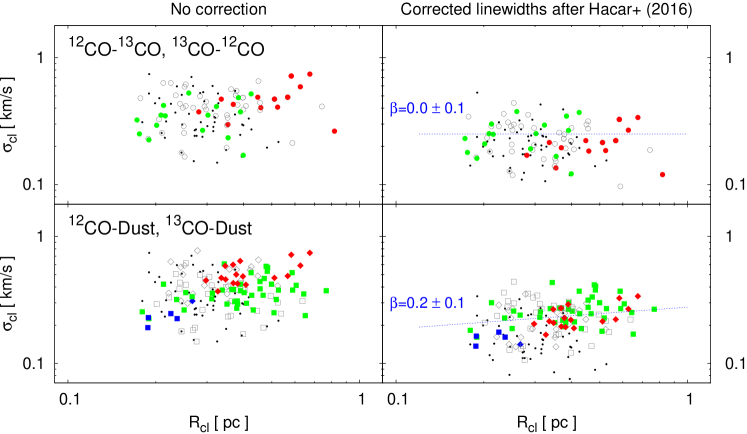
Figure 7: Diagram size vs. velocity dispersion for the clumps seen in ¹²CO or ¹³CO. The symbols are the same as in Fig. 4. The upper plots show the associations of ¹²CO and ¹³CO clumps and the lower plots – the associations of ¹²CO/¹³CO with dust clumps. The left column represents the velocity dispersions calculated from the measured linewidths, the right column gives those after the optical depth correction following Hacar et al. (2016), and the obtained slope for all associated (Types O+E) clumps.

The virial parameter of a cloud or clump is defined as

$$\alpha_{\rm vir}=\frac{5\sigma_{\rm cl}^{2}R_{\rm cl}}{GM_{\rm cl}}~{},$$ (5)

with the velocity dispersion $\sigma_{\rm cl}$ and $G$ as the gravitational constant when assuming spherical geometry and constant density. It is often used as a tool to assess gravitational boundedness of objects – those with $\alpha_{\rm vir}<2$ are considered bound (McKee & Zweibel, 1992; Ballesteros-Paredes, 2006).

A critical parameter is the velocity dispersion $\sigma_{\rm cl}=\Delta v_{\rm cl}/(2\sqrt{2\ln 2})$ that can be measured through the linewidth for all ¹³CO and ¹²CO clumps. Exploiting the strength of the clump associations we can also transfer the information on the velocity dispersion from the CO clumps to the dust clumps for which a direct measurement is impossible. The left column of Fig. 7 shows the velocity dispersions of the associated ¹²CO and ¹³CO clumps vs. their sizes. We find an offset of the dispersion of the ¹²CO clumps relative to the ¹³CO clumps. In particular the ¹²CO clumps that are associated with dust have a higher velocity dispersion than the corresponding ¹³CO clumps. The offset can be easily explained by optical depth broadening (see e.g. Phillips et al., 1979).

A correction of the optical depth broadening can be performed following Hacar et al. (2016). Those authors solved the radiative transfer equation for a Gaussian distribution of emitters in a homogeneous medium with optically thick conditions and derived a relation between the width of a Gaussian fit to an optically thick line and the width of the corresponding optically thin Gaussian profile as a function of the optical depth. In real clouds the velocity distribution may not be Gaussian, consisting of multiple velocity components along the line of sight. Nevertheless, their model matches our Gaussclumps approach of decomposing the emission into Gaussian components that are treated separately. The test presented in Appendix A.1 confirms that we obtain a self-consistent picture when the correction after Hacar et al. (2016) is applied to the individual Gaussian velocity components. This correction is derived from their relation between the width of a Gaussian fit to an optically thick line and the width of the corresponding optically thin Gaussian profile as a function of the optical depth. A rough estimate of the optical depth can be obtained from the average $X$-factors obtained in Sect. 5.1. The theoretical limit for the $X$-factor of the $1-0$ line of CO isotopes in optically thin LTE conditions is given by the energies and Einstein coefficients of the molecules (see e.g Mangum & Shirley, 2015). Using the typical temperature in the RMC of 20 K (Schneider et al., 2010) we obtain an emissivity of $7\times 10^{-16}$ K km.s${}^{-1}/\mathrm{cm}^{-2}$ per column density of the emitter. Assuming a CO abundance $N({\rm CO})/N(\mathrm{H}_{2})=2.4\times 10^{-4}$ and an isotopic ratio $N({\rm CO})/N(^{13}\mathrm{CO})=70$ this predicts optically thin limits for the $X$-factors of $X=5\times 10^{18}~{}\mathrm{cm}^{-2}\mathrm{K}^{-1}\mathrm{km}^{-1}\mathrm{s}$ and $X_{13}=4\times 10^{20}~{}\mathrm{cm}^{-2}\mathrm{K}^{-1}\mathrm{km}^{-1}\mathrm{s}$. Assuming that the higher $X$ factors obtained in Sect. 5.1 are due to optically thick emission we find optical depths in the order of $100$ for ¹²CO and in the order of 5 for ¹³CO. Using the optical depth correction from Hacar et al. (2016) for these values indicates that the velocity dispersions of ¹²CO clumps are actually lower by a factor of about 2.2 compared to the measured ones, while for the ¹³CO clumps we should apply a correction factor of 1.4. Using these correction factors to the two linewidths we obtain a good match between the velocity dispersion measured through ¹²CO and ¹³CO (see Appendix A.1). The right column of Fig. 7 shows the relation between clump size and velocity dispersions after applying the optical depth correction factors. The offset between the dispersion measured in ¹²CO and ¹³CO clumps is completely removed so that we can be confident to have a reliable measure of the actual clump velocity dispersion.

The resulting velocity dispersions cover only a small range with an average $0.25$ km s^-1 and standard deviation of $0.06$ km s^-1. The small clumps where all three tracers are associated have velocity dispersions of about $0.13$ km s^-1. Compared to the thermal value of 0.08 km s^-1 at 20 K, these are only slightly suprathermal. As there is no offset in the velocity dispersion between ¹²CO and ¹³CO clumps with and without association to dust clumps we do not expect any fundamental difference between them so that we can use the velocity dispersion measured in the molecular lines to assess the virial stability of all of the associated dust clumps.

The size-linewidth diagram of all associations of ¹²CO and ¹³CO clumps and those of CO clumps with dust counterparts (top right and bottom right panels of Fig. 7, respectively) indicates a very weak relation. When fitting the velocity scaling relation $\sigma_{\rm cl}\propto R_{\rm cl}^{\beta}$ we obtain $\beta=0$ for the ¹²CO-¹³COassociations. Interestingly, if one considers only the embedded clump populations (Type E) the scaling index $\beta$ increases up to 0.7, though the scatter is large – see last column of Table 4. This behaviour could be indicative of their evolutionary state as we comment in Sect. 7. For clumps associated with dust the fit finds a weak size dependence of $\beta=0.2$. The lack of a velocity scaling relation for the ¹²CO and ¹³CO clumps is in line with their constant density. If we assume that the region is dominated by a global large-scale velocity field and the turbulence dissipation is a function of the gas density all clumps with the same density should have about the same velocity dispersion.

5.4.2 Relationship virial parameter vs. mass

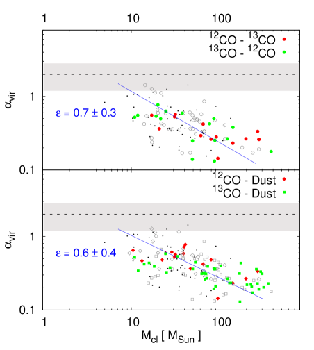
Figure 8: Virial analysis of the associated populations from diagram mass vs. virial parameter. The notation is the same like in Fig. 4. The slope for all associated clumps (Types O+E) is plotted (see text and Table 4). Shaded area demarcates the effect of possible mass uncertainties on the assessment of clump boundedness ($\alpha_{\rm vir}\gtrless 2$). Non-associated ¹²CO and ¹³CO clumps (black dots) are shown for comparison.

As evident from Fig. 8 and taking into account the assumed mass uncertainties, all associated CO clumps in the RMC are assessed as bound. The evolutionary state of the clumps can be characterised by the relation between virial parameter and mass, assumed to be a power law: $\alpha_{\rm vir}\propto M_{\rm cl}^{-\epsilon}$ (Bertoldi & McKee, 1992; Dib et al., 2007; Shetty et al., 2010). It is also recovered from combination of the mass-size relationship with power index $\gamma$ with a scaling relation of the velocity dispersion $\sigma_{\rm cl}\propto R_{\rm cl}^{\beta}$ which yields:

$$\epsilon=1-\frac{2\beta+1}{\gamma}~{}~{}.$$ (6)

In Table 4 we give the slopes obtained by direct fitting of the samples in Fig. 8. They are consistent with the values calculated from equation 6. Generally, the slope obtained for the embedded populations (Type E) seems to be shallower than the one when all associated clumps (Types O+E) are considered; while both fall within the range of estimates in star-forming regions sampled and explored by Kauffmann, Pillai & Goldsmith (2013, see Table 2 there). We note that the obtained $\epsilon\sim 0.6-0.7$ should not be interpreted as indicative for pressure-confined clumps, though similar to $\epsilon=2/3$ derived by Bertoldi & McKee (1992) on this assumption. Virial parameters below unity point to substantial role of self gravity.

Table 4: Scaling indices of virial parameter in respect to mass for the associated populations as derived directly from the diagram $M_{\rm cl}$ vs. $\alpha_{\rm vir}$ (column 3) and calculated from the scaling relations of mass and density (column 4). The slope $\beta$ of the relationship size vs. velocity dispersion is given for comparison.

12CO-13CO, 13CO-12CO
	Type	$\epsilon$	$\epsilon_{\rm calc}(\beta,\,\gamma)$	$\beta$
	O + E	$0.7\pm{\scriptstyle 0.3}$	$0.7\pm{\scriptstyle 0.2}$	$0.0\pm{\scriptstyle 0.1}$
	E	$0.3\pm{\scriptstyle 0.1}$	$0.2\pm{\scriptstyle 0.2}$	$~{}0.7\pm{\scriptstyle 0.3}$
12CO-Dust, 13CO-Dust
	Type	$\epsilon$	$\epsilon_{\rm calc}(\beta,\,\gamma)$	$\beta$
	O + E	$0.6\pm{\scriptstyle 0.4}$	$0.5\pm{\scriptstyle 0.1}$	$0.2\pm{\scriptstyle 0.1}$
	E	$0.3\pm{\scriptstyle 0.1}$	$0.2\pm{\scriptstyle 0.2}$	$0.7\pm{\scriptstyle 0.2}$

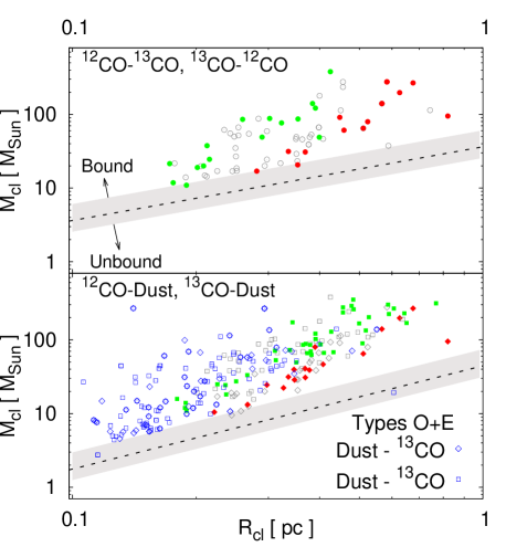
Figure 9: Virial analysis of the associated populations from mass-size diagrams. The notation of the CO populations (filled symbols for Type E, open - for Type O) is the same as in Fig. 4. Dashed line shows the virial mass $M_{\rm cl}(\alpha_{\rm vir}=2)$ as function of size, assuming velocity scalings as in Fig. 7, right; shaded area denotes its uncertainty due to uncertainty of $\alpha_{\rm vir}$ (cf. Fig. 8).

One may use the mass-size diagram as an additional tool to assess clump boundedness. From equation 5 we define the virial mass of a clump as $M_{\rm cl,\,vir}\equiv M_{\rm cl}(\alpha_{\rm vir}=2)=5\sigma_{\rm cl}^{2}R_{\rm cl}/2G$. Adopting scaling relation $\sigma_{\rm cl}\propto\sigma_{0}(R_{\rm cl}/1~{}{\rm pc})^{\beta}$, the clump virial mass scales as $M_{\rm cl,\,vir}\propto R_{\rm cl}^{2\beta+1}$. Fig. 9 displays the mass-size diagrams of associated CO clumps with plotted $M_{\rm cl,\,vir}(R_{\rm cl})$, assuming $\beta=0$ and taking $\sigma_{0}=0.25$ km s^-1 which is the average velocity dispersion for this population (cf. Fig. 7). Apparently, the line $M_{\rm cl}=M_{\rm cl,\,vir}$ could serve as a lower mass limit of the bound clump population. Thus we use it to assess also the boundedness of dust clumps (Fig. 9, bottom) for which no velocity information is available. In that vein, the association of dust clumps with CO counterparts enables their stability analysis – all but a few are classified as bound objects.

6 Clump mass functions

Clump mass functions (CMFs) are of particular interest because they could shed light on the origin of the stellar initial mass function (IMF). Below we present the derived CMFs in the RMC and probe their dependence on tracer, spatial association and the applied method to fit their high-mass parts.

The high-mass end of the CMF is usually represented through a power-law function ${\rm d}\,N_{\rm cl}/{\rm d}\,\log M_{\rm cl}\propto M_{\rm cl}^{\Gamma}$ above some characteristic mass $M_{\rm ch}$ (see e.g. Stutzki & Güsten, 1990; Heithausen et al., 1998; Kramer et al., 1998; Reid et al., 2010; Veltchev, Donkov & Klessen, 2013). However, the slope $\Gamma$ obtained from least-squares fit (LSF) is sensitive to the choice of bin size, sample size and $M_{\rm ch}$. In contrast, the maximum-likelihood (ML) fitting approach implemented in the method Plfit by Clauset et al. (2009) yields simultaneously $\Gamma$ and $M_{\rm ch}$ from the analysis of unbinned observational sample and provides a good precision for samples with $>50$ objects. The clump samples in the present study are rich enough (cf. Table 1) to allow for the application of both methods.

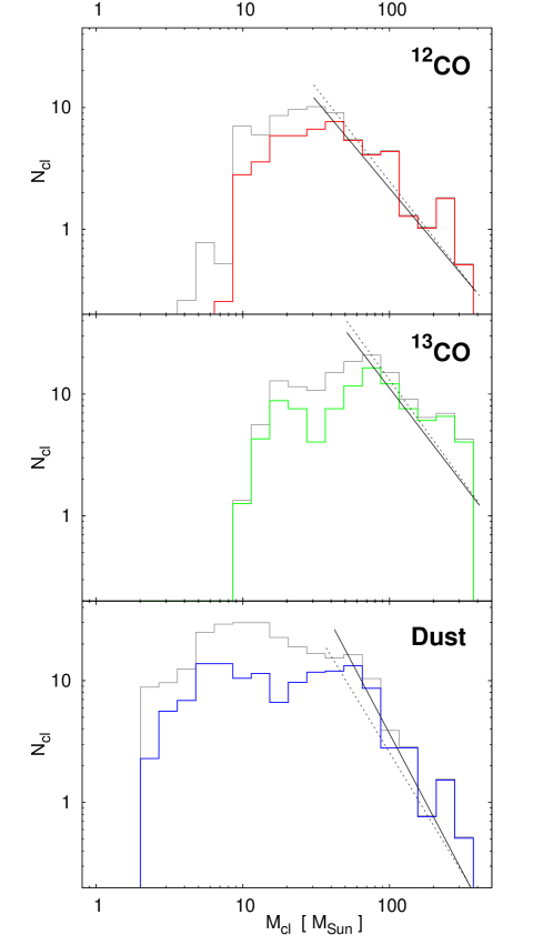
Figure 10: Mass functions of all clumps (grey) and associated clumps (colour) from a given tracer. The high-mass slopes derived through maximum-likelihood fitting for all clumps (dashed) and for the associated ones (solid) are plotted – see Table 5.

Information on the derived mass functions of the ¹²CO, ¹³CO and dust clump populations is given in Table 5 and is illustrated in Fig. 10. In general, each distribution peaks close to the characteristic mass estimated from Plfit and we adopted the latter as well in the LSF case. The non-associated clumps from all tracers contribute only to the low-mass part of the CMF.

The obtained values of $\Gamma$ from both methods are similar while the ML fitting tends to yield steeper slopes. The slopes of the CO mass functions are close to the Salpeter IMF value $-1.3$ (Salpeter, 1955) – also, when the full samples are considered. In contrast, the CMF of the dust clump population exhibits a substantially steeper slope.

Several previous studies of the RMC included the derivation of the clump mass function – in part by use of the same tracer and in a comparable mass range. All of them produced shallow slopes of a single power-law distribution, without a characteristic mass. Williams, Blitz & Stark (1995) applied the Clumpfind algorithm to ¹²CO and ¹³CO maps and obtained a slope as shallow as $\Gamma=-0.27$ in mass range $10\lesssim M_{\rm cl}/M_{\odot}\lesssim 4000$. They noticed, however, that only a few clumps from their sample are star-forming. Schneider et al. (1998) derived $\Gamma=-0.6$ for Gaussian CO clump populations extracted both from KOSMA ($14\leq M_{\rm cl}/M_{\odot}\leq 1743$) and IRAM ($3\leq M_{\rm cl}/M_{\odot}\leq 50$) maps. Their virial analysis shows that a very small fraction of the objects are gravitationally bound. Extracting clumps from Herschel maps through the technique Getsources and identifying them with young stellar sources from Spitzer, Di Francesco et al. (2010) investigated separately samples of prestellar ($10\leq M_{\rm cl}/M_{\odot}\leq 300$) and starless ($2\leq M_{\rm cl}/M_{\odot}\leq 200$) cores. In both cases, a slope $\Gamma\simeq-0.8$ was obtained as the distribution peaks have been taken as characteristic masses and no assessment of the gravitational boundedness has been made. In terms of tracer and data source, our work on the dust population is comparable with that of Di Francesco et al. (2010). The much shallower $\Gamma$ found by those authors could be attributed to the applied different method for clump extraction and/or to the use of a single fit. If we adopt as a characteristic mass the mass-distribution peak for all dust clumps at $\sim 10~{}M_{\odot}$ (cf. Fig. 10, bottom), the corresponding slope is $\Gamma\simeq-0.7$ – in agreement with the work of Di Francesco et al. (2010). Also, the results from both studies could reflect the lack of high-enough angular resolution to resolve clumps with sizes below $R_{\rm cl}\simeq 0.2$ pc; cf. our Fig. 5 (bottom) and Fig. 2 in Di Francesco et al. (2010). This size range roughly corresponds to masses $M_{\rm cl}\lesssim 20$  $M_{\odot}$(Fig. 4).

Table 5: Parameters of clump mass functions from different tracers. Abbreviations of the fitting methods: ML - Maximum Likelihood, $D$ - Kolmogorov-Smirnov statistic of ML-fit goodness, LSF - weighted least-squares fit with logarithmic bin size $1.3$ and Poissonian error. The characteristic masses are taken from the ML output and given in solar units.

Tracer	All clumps				All associated clumps
	ML			LSF	ML			LSF
	$M_{\rm ch}$	$D$	$-\Gamma$	$-\Gamma$	$M_{\rm ch}$	$D$	$-\Gamma$	$-\Gamma$
12CO	$34$	$0.09$	$~{}1.5$	$1.2\pm{\scriptstyle 0.1}$	$34$	$0.09$	$1.4$	$1.1\pm{\scriptstyle 0.2}$
13CO	$66$	$0.10$	$~{}1.6$	$1.2\pm{\scriptstyle 0.1}$	$66$	$0.12$	$1.6$	$1.1\pm{\scriptstyle 0.2}$
Dust	$44$	$0.05$	$~{}2.0$	$1.5\pm{\scriptstyle 0.2}$	$50$	$0.07$	$2.3$	$2.3\pm{\scriptstyle 0.3}$

7 Discussion

Possible caveats of the presented study are the uncertainties in the column-density maps and superposition effects. We find an average value for the $X$ factor that is somewhat higher than the Galactic average. Nevertheless, it gives realistic and self-consistent estimates of the masses of the embedded clump populations (Fig. 3). We adopt also average uncertainties of size and mass estimates due superposition effects (Beaumont et al., 2013). Individual uncertainty may vary with size; smaller clumps which are deeply embedded in cloud material are more susceptible to superposition. Objects of lower mean brightness could also misrepresent the real structure in the PPP space. However, such clumps do not affect the result on the mass scaling of the associated CO populations and, also, are not taken into account to derive the high-mass CMF.

Most molecular-line investigations of Galactic star-forming regions, by use of different clump-extraction techniques, result in mass scaling indices $\gamma$ close to $2$ or a few dex larger (see Veltchev, Donkov & Klessen, 2013, Table 1). This is reproduced from the derived mass-size relations in this work as far as all clumps from the considered population are taken into account (Table 3, column 2). The surprising result is the single steep mass scaling relation $\gamma\simeq 3$ of the associated CO clumps, which corresponds to objects of constant mean volume density. How could one interpret this finding? Below we suggest a possible explanation from features of the CO detection and involving a model for clumps which are about to form stars.

Critical density for excitation of CO molecules can explain the behaviour of associated clumps from these tracers. It gives us access to their nature that goes beyond the purely statistical result of a decomposition algorithm. The constant density of the CO clump associations is in line with the small dynamical range in densities that an individual molecular line is sensitive to (see e.g. Schneider et al., 2016). At lower densities the molecule is only subthermally excited, at higher densities it becomes quickly optically thick (Draine, 2011; Klessen & Glover, 2015). The density variation of the associated clumps probably stems from the different optical depths while both isotopes have about the same critical density for the collisional excitation. Hence, we can conclude that all associated CO clumps are real physical objects with at least the inferred density from Fig. 4. In contrast, every non-biased clump decomposition mechanism tends to find clumps with constant column density (see e.g. Heyer et al., 2009). A fixed noise threshold and dynamic range of a map provide natural limits to the derived column density; an illustration for our clump samples is provided in the Appendix, Fig. 12. With Gaussclumps larger structures can still be identified at average columns below the noise threshold of individual pixels so that we naturally expect a clump scaling exponent somewhat above two, in line with our values for the individual maps of $\gamma\approx 2.4$. The fact that associated dust clumps also show a steeper exponent indicates that the associations bias the dust clump sample to clumps with densities above the CO critical density, but – as there is no upper limit for the measured column in the dust maps – they can go towards higher densities. Most dust clumps can be regarded as the “tips of the iceberg” on top of the CO clumps, as seen through the types of embeddedness in Table 2 and Fig. 4. Most dust clumps are embedded in CO clumps having significantly smaller radii. Hence, we can use the associations as a tool to identify significant physical entities above a certain density threshold.

The mean density of the associated CO clumps is about $3-8\times 10^{3}$ cm^-3 while dust emission as an optically thinner tracer allows for identification of their counterparts with $3\times 10^{3}\lesssim\langle n\rangle\lesssim 10^{5}$ cm^-3 (Fig. 4, bottom). The shallower index $\gamma\sim 2.5$ obtained for the sample of associated dust clumps, combined with the significantly larger scatter could be attributed to the lack of single density scaling law at scales below few $0.1$ pc – the mass of structures of one and the same size could vary by orders of magnitude (Falgarone et al., 1992; Hennebelle & Falgarone, 2012).

Another interesting result from our work is the virtual lack of a velocity-size relation for the associated CO clumps (Fig. 7). It is consistent with the findings from a number of studies of clumps with similar size and with similar to higher densities in star-forming regions (Casseli & Myers, 1995; Shirley et al., 2003; Gibson et al., 2009; Wu et al., 2010). We suggest an interpretation provided from the recent simulations of evolving MCs in a typical Galactic environment by Ibáñez-Mejía et al. (2016). In their work, the identified structures of low density $\langle n\rangle\leq 5\times 10^{3}$ cm^-3(i.e. traceable by CO emissions) display no dependence of the velocity dispersion with radius at early evolutionary phases, prior to the onset of self-gravity. This fact, along with the measured $0.35~{}{\rm kms}^{-1}\leq\sigma\leq 0.6$ km s^-1, is explained with the formation of the considered objects through compression by converging flows. Their low velocity dispersions determine bound states: $\alpha_{\rm vir}$ less than $0.5$ and scaling with mass by $\epsilon\sim 0.7$, in agreement with our results for all associated clumps in Sect. 5.4.2. On the other hand, further evolution of these clouds is affected strongly by self-gravity and leads to an increase of their velocity dispersions – a linewidth-size relation appears, with index $\beta$ as high as $0.62\pm 0.12$ (see Fig. 9 in Ibáñez-Mejía et al. 2016). Interestingly, such behaviour is found from virial analysis of our embedded clump populations (Table 4). Whether this is indicative of their evolutionary state is speculative. A cross-identification with mapped young stellar sources and/or prestellar cores might shed light on this issue.

The derived CMFs of the CO populations exhibit steep slopes in their high-mass parts, comparable to or larger than the one of the stellar IMF. Such slopes of $\Gamma$ are not exceptional – similar values are derived from studies of other Galactic star-forming regions (see review and the references in Veltchev, Donkov & Klessen, 2013), adopting $M_{\rm ch}\gtrsim 10~{}M_{\odot}$ to separate intermediate-mass from high-mass part. In the cited work the observational CMFs were successfully modelled from statistical description of clump ensembles under the assumption of multi-scale, virial-like equipartition between gravitational and turbulent energy. In regard to this, we note again that the vast majority of the RMC clumps are found to be gravitationally bound by the performed virial analysis (Sect. 5.4).

8 Summary

We study clump populations extracted from ¹²CO, ¹³CO and Herschel dust-emission maps of the Rosette molecular cloud (RMC) using the clump-extraction algorithm Gaussclumps. By performing a cross-identification (association) between the populations from different tracers and subsequent physical analysis we can derive essential properties of the cloud structure:

• Clump associations allow us to combine the information on the physical properties of the clumps that are measured by the different tracers. The assignment of the tracers to the same material is most reliable at scales of large cross-correlation coefficients, favouring the larger clumps in our study. By comparing clump masses we obtain a reliable estimate for the $X$ factors translating ¹²CO and ¹³CO intensities into column densities ($X=4\times 10^{20}~{}\mathrm{cm}^{-2}\mathrm{K}^{-1}\mathrm{km}^{-1}\mathrm{s}$, $X_{13}=3\times 10^{21}~{}\mathrm{cm}^{-2}\mathrm{K}^{-1}\mathrm{km}^{-1}\mathrm{s}$). After correction for optical depth broadening we obtain a reliable measure for the velocity dispersion in the gaseous clumps that can be transferred to the dust clumps that have no separate velocity information.

• The associated Gaussian clumps extracted from CO tracers obey a single mass-size relation $M_{\rm cl}\propto R_{\rm cl}^{3}$ which implies approximately constant mean density about $3\times 10^{3}$ cm^-3(¹²CO) and $6-8\times 10^{3}$ cm^-3(¹³CO). This behaviour can be explained by the small dynamical range in densities to which an individual molecular line is sensitive.

• The associated Gaussian clumps extracted from Herschel dust-emission map are usually embedded within the larger CO clumps representing their density peaks at scales a few tenths of pc where no single density scaling law (and no single mass-size relationship, respectively) is expected. This is reflected in a shallower mass scaling (slopes about $2.5$) than their CO associates.

• All associated CO clumps (and all but a few of their dust counterparts) are assessed to be gravitationally bound and their location delineates the massive star-forming filaments and their junctions studied by Schneider et al. (2012). They display virtually no velocity-size relation, in consistence with the derived relation between their masses and virial parameters. We interpret this behaviour as indicative of low-density clumps formed through compression by converging flows and still not evolved under the influence of self-gravity.

• The derived mass functions of the CO clump populations (associated or not) display a nearly Salpeter slope ($\Gamma\sim-1.3$), corresponding to the high-mass slope of the stellar initial mass function. In contrast, the mass functions of the dust clump populations are much steeper ($\Gamma\lesssim-2$).

Acknowledgement: We are grateful to M. Heyer and J. Williams who graciously provided us with the FCRAO molecular-line maps of the Rosette region. We thank as well J. Ballesteros-Paredes for the helpful discussion on some results from this study and to the anonymous referee who’s suggestions helped us to improve the readability of the paper.

This work was realised within the bilateral partnership agreement between the University of Sofia and the University of Cologne, part of the Priority program 1573 of the Deutsche Forschungsgemeinschaft (DFG). T.V. acknowledges partial support by the DFG under grant KL 1358/20-1 and V.O. and N.S. acknowledge support by the DFG under grant OS 177/2-2. R.S.K. thanks funding from the DFG in the Collaborative Research Center (SFB 881) ”The Milky Way System” (subprojects B1, B2, and B8) and in the Priority Program SPP 1573 ”Physics of the Interstellar Medium” (grant numbers KL 1358/18.1, KL 1358/19.2).

Appendix A Characteristics of associated clump populations

Tables 6, 7 and 9 provide full lists of the associated clumps and their physical parameters. The sizes of the associated objects from each pair of tracers are juxtaposed in Fig. 11. Embedded clumps (Types E1 or E2) are separated by the identity line per definition. In average, ¹²CO clumps are about twice larger than their ¹³CO embedded associates. The correlation of sizes of embedded ¹²CO/¹³CO - dust pairs is weaker.

The distribution of mean surface densities for associated and non-associated clump populations from different tracers are plotted in Fig. 12.

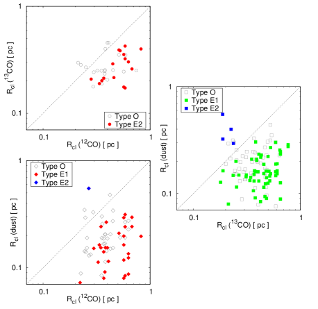
Figure 11: Sizes of associated Gaussian clump pairs, extracted from different tracers.

Figure 12: Distribution of mean surface density of clumps, extracted from different tracers. The solid lines show the distribution of clumps associated with any other tracer, the dashed lines those of non-associated clumps.

Table 6: List of all associated ¹²CO clumps.

#	$l$	$b$	Axis 1	Axis 2	Orient. angle	Size	Mass	$\sigma$	13CO ass.	Dust ass.
	[deg]	[deg]	[″]	[″]	[deg]	[pc]	[ $M_{\odot}$]	[km s-1]
1	207.023926	-1.820533	74.6	109.7	32.3	0.5833	276.5	1.69	1, 24, 80	10, 11, 34, 52, 282
2	206.946793	-1.811981	81.7	115.5	153.1	0.6266	197.2	1.39	5	56, 78, 80, 177, 239
4	207.323105	-2.163783	62.4	124.1	64.5	0.5671	140.1	1.15	2, 116, 156	4, 26, 44, 117, 166
7	206.992935	-1.782242	48.7	78.3	165.2	0.3981	66.6	1.14	3, 182	39, 286
8	206.912140	-1.869369	56.0	117.8	147.0	0.5236	79.5	0.96	56	187
10	206.945114	-1.638992	43.5	100.0	66.3	0.4251	92.9	1.36	–	63, 224
11	207.027939	-1.792006	76.9	47.5	170.8	0.3897	79.8	1.51	–	52
12	207.394547	-1.941092	55.3	87.2	55.7	0.4477	91.0	1.15	41	38
16	206.905518	-1.916839	88.4	57.2	174.0	0.4585	61.0	0.95	179	–
18	207.121262	-1.881081	39.0	89.8	30.4	0.3817	53.2	1.00	11	14, 45, 163
22	206.951279	-1.593222	45.8	106.4	112.4	0.4502	113.5	1.54	85	57, 131
23	206.893539	-1.799839	36.4	94.8	133.6	0.3785	49.1	1.29	109	107, 148
26	206.794785	-1.772153	177.1	62.0	8.2	0.6756	267.4	1.75	23	71, 249
33	206.977036	-1.837939	81.4	45.3	138.1	0.3917	38.6	1.06	–	60
34	207.425369	-1.961631	63.3	63.2	173.4	0.4077	46.5	0.98	9	92
36	207.049423	-1.800294	32.7	103.9	58.6	0.3760	38.9	1.19	18, 42	–
37	206.923096	-1.887656	45.7	65.8	128.3	0.3536	20.7	0.70	124	257
42	207.093842	-1.870303	68.6	43.2	21.0	0.3511	29.1	0.83	66	281
57	206.923035	-1.846186	32.9	46.1	121.4	0.2510	18.6	1.39	61	328
60	207.028488	-1.838747	29.5	86.9	39.5	0.3266	22.3	0.87	–	89
63	206.872894	-1.840867	40.4	78.4	72.8	0.3628	45.8	1.33	302	–
64	207.455322	-1.968656	43.2	62.7	30.9	0.3356	31.4	1.11	251	293
66	207.154510	-1.878117	89.2	33.8	20.5	0.3541	28.8	0.96	–	15
74	207.305466	-2.156178	49.1	66.7	39.9	0.3689	30.8	1.01	62	26
79	207.188660	-1.926303	49.9	49.7	175.3	0.3211	21.7	0.82	149	–
81	207.000488	-1.774714	73.2	39.4	72.1	0.3463	39.4	1.38	–	286
91	207.272141	-1.810972	46.7	69.9	76.9	0.3683	40.8	1.41	–	1, 6, 7
96	207.314346	-2.102122	46.6	94.7	39.2	0.4284	57.5	1.21	–	–
102	207.078812	-1.876608	28.6	55.6	73.6	0.2572	10.8	0.70	–	65, 149
103	207.066910	-1.848575	42.0	28.1	152.2	0.2215	10.4	0.84	–	271
107	207.429016	-1.994303	41.5	41.4	14.0	0.2670	13.2	0.73	–	66
119	206.851364	-1.798392	37.0	50.2	129.3	0.2779	34.4	1.82	–	236
125	207.071335	-1.782483	70.4	43.7	13.4	0.3577	38.6	1.30	–	41
128	207.156860	-1.915303	28.8	66.1	42.8	0.2810	17.0	0.88	309	–
143	207.222549	-1.637233	34.3	60.6	122.1	0.2938	20.0	0.97	270	61
151	207.228317	-2.461564	152.8	54.5	160.5	0.5882	37.6	0.50	78	–
152	207.122803	-1.639314	65.2	32.6	145.1	0.2975	24.4	1.06	57	251
158	206.854767	-1.750297	109.9	38.9	57.5	0.4213	56.6	1.28	–	153
160	207.183746	-2.245544	243.2	54.6	165.1	0.7431	114.0	0.97	154	–
173	207.311600	-2.155100	46.0	32.2	1.9	0.2480	17.5	1.18	–	4
190	207.219101	-1.611764	34.3	31.6	21.3	0.2123	14.3	1.49	118	–
194	207.005981	-1.927936	37.9	37.8	151.0	0.2442	9.5	0.73	–	305
200	207.349304	-2.305289	75.4	215.0	82.9	0.8209	95.0	0.62	98	201
210	207.317719	-1.900606	42.9	69.8	43.3	0.3529	23.3	0.79	148	–
218	206.910721	-1.677203	25.6	55.8	74.5	0.2437	19.1	1.35	–	219
221	206.950302	-1.560703	32.1	38.0	103.0	0.2252	17.0	1.49	45	169
227	206.799850	-1.763731	82.1	35.3	143.4	0.3473	28.7	1.08	–	249
262	207.676910	-1.555356	45.6	137.7	100.8	0.5109	64.8	1.11	46, 258	69
308	207.300903	-2.127922	44.3	77.5	49.2	0.3777	38.9	1.18	–	337
376	207.123428	-1.621158	34.3	50.5	151.8	0.2682	12.6	0.83	–	338

Table 7: List of all associated ¹³CO clumps.

#	$l$	$b$	Axis 1	Axis 2	Orient. angle	Size	Mass	$\sigma$	12CO ass.	Dust ass.
	[deg]	[deg]	[″]	[″]	[deg]	[pc]	[ $M_{\odot}$]	[km s-1]
1	207.017502	-1.815992	40.92	106.09	44.1	0.4248	380.0	1.22	1	10, 282
2	207.322815	-2.167897	38.79	77.76	47.5	0.3542	86.4	0.55	4	117
3	206.988449	-1.784817	127.71	39.13	171.2	0.4558	274.6	1.04	7	39, 286
5	206.939468	-1.809586	51.31	42.77	8.0	0.3021	87.6	0.83	2	56
6	207.127731	-1.835806	89.29	62.76	34.2	0.4827	350.1	1.25	–	211
7	207.284317	-2.148969	68.38	47.76	3.9	0.3685	141.5	0.90	–	111
8	207.560471	-1.713642	86.50	61.72	165.6	0.4711	240.2	1.10	–	25, 137
9	207.423874	-1.951617	135.91	36.78	23.7	0.4559	234.1	0.91	34	92
11	207.128937	-1.875972	85.09	45.17	11.4	0.3998	178.0	0.92	18	319
15	207.294266	-2.092403	43.07	54.01	29.6	0.3110	102.5	0.97	–	40
18	207.045258	-1.817914	31.35	42.06	122.7	0.2341	61.5	1.19	36	34
19	207.259964	-1.812581	60.77	92.63	141.2	0.4838	257.6	1.34	–	1, 7, 64, 242
20	206.996277	-1.816097	44.21	52.78	87.8	0.3114	70.9	0.76	–	60
21	206.870819	-1.874375	43.96	64.56	84.6	0.3435	172.7	1.43	–	20
23	206.797562	-1.770117	33.51	48.37	25.3	0.2596	85.2	1.24	26	–
24	207.012497	-1.822536	23.50	30.41	43.5	0.1724	21.3	0.76	1	–
25	206.908569	-1.784900	55.99	40.10	168.4	0.3055	100.2	1.13	–	222
28	207.067215	-1.814750	63.87	86.20	147.3	0.4784	287.7	1.37	–	22
30	207.290100	-2.188197	92.71	47.29	7.0	0.4269	128.0	0.81	–	43
34	207.310562	-1.822886	115.00	72.71	12.1	0.5896	223.3	0.89	–	23, 101, 160, 364
35	207.307831	-2.132703	41.21	83.83	105.9	0.3790	85.1	0.64	–	337
37	207.154877	-1.880883	81.50	101.70	160.5	0.5871	298.8	1.22	–	15, 51, 319
41	207.390228	-1.946653	39.24	51.37	25.7	0.2895	48.9	0.63	12	–
42	207.036850	-1.788664	27.32	54.04	28.0	0.2477	49.8	0.95	36	–
44	207.316818	-1.877236	31.34	76.33	30.6	0.3154	66.3	0.89	–	67
45	206.949249	-1.564369	30.21	64.12	87.8	0.2838	87.1	1.17	221	169
46	207.676697	-1.557078	38.90	94.31	94.8	0.3905	121.0	0.88	262	69
47	207.589127	-1.758081	38.83	82.22	55.0	0.3643	85.1	0.90	–	12
48	207.144730	-1.821492	59.10	88.71	121.4	0.4669	119.2	0.81	–	47
49	207.082047	-1.866792	76.03	116.36	111.3	0.6065	265.1	0.97	–	19, 65, 149
50	207.210541	-1.835375	46.60	59.03	158.2	0.3382	72.6	0.89	–	46
51	207.286285	-2.424056	59.84	79.79	130.1	0.4456	109.3	0.61	–	198
52	207.183502	-1.783253	49.66	66.20	145.3	0.3697	88.0	0.90	–	9, 183, 358
54	207.782776	-1.784194	63.08	110.68	87.7	0.5388	116.6	0.58	–	104
56	206.905136	-1.871392	39.42	90.14	141.8	0.3843	140.0	1.14	8	–
57	207.108276	-1.642528	26.91	52.42	116.9	0.2422	55.1	1.02	152	251
59	207.172119	-1.845550	54.06	73.01	23.2	0.4051	96.3	0.89	–	194
61	206.922104	-1.841356	32.72	53.15	62.2	0.2689	54.4	0.95	57	–
62	207.304169	-2.155556	45.78	23.75	15.4	0.2126	37.5	0.99	74	4, 26
65	207.105698	-1.808583	35.70	42.22	93.6	0.2503	27.3	0.62	–	98
66	207.089584	-1.866308	47.54	31.48	1.8	0.2494	34.8	0.68	42	–
69	207.304062	-2.532933	114.89	58.13	9.2	0.5270	201.5	0.89	–	21, 128
71	207.344818	-1.948906	23.89	32.51	59.6	0.1797	15.9	0.60	–	243
72	207.360107	-1.945022	26.36	46.31	71.0	0.2253	24.9	0.58	–	84
78	207.243835	-2.449700	35.08	84.04	149.0	0.3501	46.0	0.46	151	–
79	207.277222	-1.864947	45.17	142.92	11.5	0.5181	133.1	0.75	–	208, 366
80	207.027939	-1.828756	63.65	39.44	173.5	0.3230	76.2	0.97	1	–
81	207.317184	-1.838792	64.89	49.17	20.0	0.3642	69.2	0.73	–	24, 109
85	206.935623	-1.601728	26.51	58.29	122.8	0.2535	51.5	0.98	22	131
87	207.826660	-1.849742	72.84	140.08	140.4	0.6513	168.1	0.56	–	29, 95, 195, 318
91	207.367767	-1.849053	56.38	110.39	53.2	0.5087	89.3	0.59	–	171
92	207.206085	-1.866494	103.14	33.78	160.4	0.3806	69.6	0.73	–	336
93	207.586731	-1.727814	65.47	59.35	23.7	0.4020	86.3	0.85	–	139
94	207.700165	-1.920394	152.63	65.29	179.6	0.6437	228.4	0.83	–	49
96	207.361786	-1.904942	49.50	74.21	30.9	0.3908	102.3	0.99	–	180
98	207.343964	-2.297911	66.36	57.77	18.6	0.3992	48.8	0.40	200	201
99	207.299927	-1.801072	57.88	103.53	161.3	0.4991	166.2	0.99	–	48, 261, 294
100	207.554169	-1.753769	52.07	70.92	69.6	0.3918	95.6	1.01	–	168
103	207.330521	-2.350303	44.85	44.88	123.2	0.2893	38.5	0.62	–	241
104	207.072906	-1.796483	27.39	56.46	92.9	0.2535	38.4	0.85	–	41, 360
106	207.788742	-1.878017	104.28	136.30	73.8	0.7687	311.4	0.88	–	59, 205

Table 8: continued

#	$l$	$b$	Axis 1	Axis 2	Orient. angle	Size	Mass	$\sigma$	12CO ass.	Dust ass.
	[deg]	[deg]	[″]	[″]	[deg]	[pc]	[ $M_{\odot}$]	[km s-1]
109	206.884689	-1.796822	28.75	53.76	122.8	0.2535	66.3	1.45	23	148
111	207.572250	-1.711033	103.15	43.55	159.0	0.4322	67.8	0.62	–	8
114	207.266602	-1.772617	33.14	51.60	80.3	0.2666	33.1	0.79	–	346
116	207.311188	-2.183314	23.50	61.47	94.8	0.2451	16.9	0.42	4	166
118	207.232056	-1.610922	35.40	60.12	122.0	0.2975	58.8	0.92	190	–
122	207.020020	-1.841539	45.00	76.75	115.8	0.3789	89.0	0.89	–	11, 89
124	206.922455	-1.882825	27.41	35.62	122.8	0.2014	18.9	0.69	37	257
126	207.231674	-1.746394	62.60	37.58	173.2	0.3127	52.7	0.84	–	260
127	207.433212	-1.983422	34.11	24.90	179.7	0.1879	11.9	0.45	–	66
129	207.083786	-1.851375	72.79	46.01	6.2	0.3732	65.6	0.72	–	19
134	207.366562	-1.783275	74.09	39.19	157.3	0.3475	67.2	0.94	–	306
140	206.931046	-1.628206	33.37	62.96	58.4	0.2955	71.4	1.09	–	33
143	207.399872	-1.378078	48.45	121.76	131.3	0.4953	126.0	0.80	–	133
148	207.327835	-1.905264	28.33	30.20	20.3	0.1886	14.0	0.54	210	108
149	207.193726	-1.922300	23.51	63.96	28.2	0.2500	26.8	0.60	79	–
150	207.891022	-1.810161	111.83	47.21	171.7	0.4685	60.0	0.45	–	273
152	207.243652	-1.566853	26.01	53.79	119.0	0.2412	38.0	0.91	–	77
154	207.145691	-2.245997	25.68	59.11	139.2	0.2512	17.0	0.39	160	–
156	207.332291	-2.166375	23.71	31.35	68.0	0.1758	11.8	0.59	4	–
158	207.645599	-1.899469	56.06	55.99	132.7	0.3613	40.7	0.56	–	130
165	207.762634	-1.927164	74.98	88.25	71.3	0.5245	108.4	0.71	–	42, 97
175	207.170944	-1.798603	46.96	85.99	126.6	0.4097	66.3	0.70	–	134
179	206.901352	-1.911522	39.46	28.30	39.6	0.2155	24.5	0.82	16	–
182	206.989166	-1.772997	36.02	28.11	169.0	0.2052	19.8	0.77	7	–
189	207.681931	-1.643536	34.10	52.33	67.3	0.2724	20.0	0.45	–	124
202	207.339600	-2.567433	45.69	76.82	64.3	0.3820	62.2	0.69	–	120
203	207.388718	-1.194906	212.27	45.99	38.8	0.6371	189.6	0.73	–	28
216	207.482956	-1.700631	38.51	45.15	83.3	0.2689	18.6	0.43	–	259
223	207.294281	-1.751072	23.79	56.71	94.4	0.2368	18.1	0.53	–	265
248	207.376724	-2.361628	34.79	38.45	105.8	0.2358	24.2	0.75	–	207
251	207.455704	-1.967514	36.34	23.74	31.7	0.1894	10.9	0.53	64	293
258	207.668015	-1.555822	30.50	97.12	91.2	0.3509	49.3	0.69	262	69
262	206.883255	-1.889175	26.83	44.40	119.3	0.2225	21.6	0.78	–	74
270	207.211227	-1.640056	31.82	23.74	165.6	0.1772	21.6	1.13	143	–
275	207.321793	-2.293533	29.75	61.60	140.5	0.2761	15.5	0.35	–	201
302	206.871368	-1.844628	23.69	44.76	73.5	0.2100	14.8	0.60	63	–
309	207.154953	-1.910250	24.03	43.51	37.9	0.2085	19.9	0.83	128	–

Table 9: List of all associated dust clumps.

#	$l$	$b$	Axis 1	Axis 2	Orient. angle	Size	Mass	12CO ass.	13CO ass.
	[deg]	[deg]	[″]	[″]	[deg]	[pc]	[ $M_{\odot}$]
1	207.263519	-1.812227	22.850	20.799	141.7	0.1405	267.7	91	19
4	207.316498	-2.152799	41.092	50.378	87.0	0.2933	266.4	4, 173	62
6	207.281265	-1.803322	21.302	39.748	123.1	0.1876	99.0	91	–
7	207.274597	-1.824577	25.311	26.595	74.0	0.1672	60.7	91	19
8	207.573730	-1.715249	36.033	35.096	110.0	0.2293	110.6	–	111
9	207.178574	-1.790581	20.194	20.500	107.4	0.1312	44.3	–	52, 175
10	207.003250	-1.809448	25.858	34.192	142.0	0.1917	69.4	1	1
11	207.019287	-1.834404	31.519	44.440	104.1	0.2413	114.2	1	122
12	207.595551	-1.762271	17.131	15.834	79.1	0.1062	26.8	–	47
14	207.112213	-1.874567	22.331	45.132	107.9	0.2047	67.2	18	–
15	207.147217	-1.880469	37.977	57.559	135.2	0.3014	135.8	66	37
19	207.080032	-1.853194	15.625	41.104	127.5	0.1634	44.6	–	49, 129
20	206.864578	-1.877663	26.845	18.099	106.5	0.1421	31.1	–	21
21	207.313156	-2.535746	18.197	31.104	97.6	0.1534	32.5	–	69
22	207.066986	-1.820135	39.235	16.165	105.2	0.1623	41.0	–	28
23	207.292053	-1.833485	28.179	30.402	76.2	0.1887	41.1	–	34
24	207.325989	-1.841186	35.372	41.370	79.3	0.2466	63.1	–	81
25	207.539764	-1.722399	20.807	23.450	138.2	0.1424	26.4	–	8
26	207.299988	-2.153447	10.363	14.769	142.4	0.0797	11.7	4, 74	62
28	207.387711	-1.200810	22.416	55.657	126.6	0.2277	56.9	–	203
29	207.820404	-1.869027	73.438	19.956	118.3	0.2468	67.5	–	87
33	206.923126	-1.625726	31.335	19.515	98.0	0.1594	28.1	–	140
34	207.038132	-1.823000	64.027	37.042	92.7	0.3140	78.9	1	18
38	207.403854	-1.945135	28.939	61.887	110.7	0.2728	62.1	12	–
39	206.980835	-1.792985	36.982	22.868	112.6	0.1875	31.2	7	3
40	207.299042	-2.089805	30.359	37.810	99.9	0.2184	44.3	–	15
41	207.068726	-1.791201	33.395	47.371	106.5	0.2564	58.3	125	104
42	207.755325	-1.936775	51.862	89.527	97.4	0.4393	140.5	–	165
43	207.292389	-2.188894	24.373	47.070	110.0	0.2184	47.0	–	30
44	207.322525	-2.136961	18.761	17.809	61.7	0.1178	14.8	4	–
45	207.123840	-1.894273	17.088	33.440	118.5	0.1541	23.1	18	–
46	207.213791	-1.837247	20.588	20.484	162.0	0.1324	16.4	–	50
47	207.153214	-1.834679	31.781	55.356	135.8	0.2704	55.0	–	48
48	207.308899	-1.805477	34.360	34.609	70.6	0.2223	40.4	–	99
49	207.693375	-1.925644	27.323	57.313	123.8	0.2551	50.2	–	94
51	207.172455	-1.884521	51.425	42.474	90.1	0.3013	65.4	–	37
52	207.020584	-1.792733	41.801	40.818	81.1	0.2663	57.7	1	–
56	206.945175	-1.817623	20.365	21.518	76.4	0.1349	11.2	2	5
57	206.945007	-1.586929	73.244	38.464	96.5	0.3422	69.8	22	–
59	207.786240	-1.859325	52.540	34.661	117.2	0.2751	51.2	–	106
60	206.988373	-1.821593	23.290	21.273	86.1	0.1435	14.9	33	20
61	207.227844	-1.624462	73.422	35.722	117.7	0.3302	72.2	143	–
63	206.933914	-1.648822	33.063	30.730	78.7	0.2055	27.6	10	–
64	207.245499	-1.808280	51.262	24.315	97.6	0.2276	33.0	–	19
65	207.075958	-1.866452	17.369	49.979	129.9	0.1899	23.6	102	49
66	207.431564	-1.985184	95.524	76.469	151.7	0.5511	138.4	107	127
67	207.308060	-1.876241	40.374	36.242	169.4	0.2466	35.5	–	44
69	207.676498	-1.556596	34.953	30.320	86.9	0.2099	27.5	262	46, 258
71	206.790985	-1.782508	35.753	58.944	106.2	0.2960	52.8	26	–
74	206.878906	-1.892263	35.983	30.359	147.9	0.2131	27.2	–	262
77	207.239197	-1.577599	65.649	33.044	130.9	0.3003	50.4	–	152
78	206.924118	-1.812391	48.701	37.169	3.5	0.2743	40.4	2	–
80	206.957672	-1.794173	45.861	27.254	126.4	0.2279	29.8	2	–
84	207.366516	-1.951482	44.769	85.544	126.0	0.3990	87.4	–	72
89	207.027054	-1.849236	14.666	20.791	134.8	0.1126	8.2	60	122
92	207.430634	-1.951102	18.764	16.838	153.5	0.1146	7.6	34	9
95	207.835007	-1.837569	26.368	49.742	127.3	0.2335	29.8	–	87
97	207.774399	-1.914737	57.055	41.598	89.2	0.3141	43.9	–	165
98	207.109055	-1.810394	34.920	27.630	173.2	0.2002	21.5	–	65
101	207.304947	-1.823945	18.227	28.587	90.6	0.1471	12.5	–	34
104	207.786575	-1.771225	66.501	44.612	92.0	0.3512	52.0	–	54

Table 10: continued

#	$l$	$b$	Axis 1	Axis 2	Orient. angle	Size	Mass	12CO ass.	13CO ass.
	[deg]	[deg]	[″]	[″]	[deg]	[pc]	[ $M_{\odot}$]
107	206.906769	-1.794024	35.791	19.090	121.8	0.1685	14.6	23	25
108	207.329880	-1.902573	40.578	62.026	95.5	0.3234	45.3	–	148
109	207.317841	-1.849597	13.726	39.271	129.8	0.1497	12.0	–	81
111	207.274780	-2.146296	54.046	48.001	148.7	0.3284	52.8	–	7
117	207.333359	-2.171435	33.985	27.641	113.9	0.1976	20.0	4	2
120	207.339050	-2.569749	50.174	44.283	103.8	0.3039	40.6	–	202
124	207.688248	-1.648921	17.702	23.262	140.1	0.1308	9.2	–	189
128	207.292252	-2.540013	42.094	41.456	162.6	0.2693	29.5	–	69
130	207.655762	-1.907992	27.191	38.539	99.2	0.2087	18.7	–	158
131	206.931473	-1.609767	21.948	25.764	155.5	0.1533	9.2	22	85
133	207.401382	-1.383992	62.297	36.012	117.1	0.3054	37.9	–	143
134	207.165543	-1.806305	29.583	44.250	98.6	0.2332	22.5	–	175
137	207.550400	-1.708699	17.785	20.706	168.7	0.1237	6.8	–	8
139	207.588120	-1.730466	29.901	20.575	138.7	0.1599	11.0	–	93
148	206.881012	-1.801407	45.481	22.142	120.8	0.2046	17.0	23	109
149	207.083038	-1.882143	16.431	34.357	117.0	0.1532	12.1	102	49
153	206.857147	-1.738360	98.238	56.385	138.7	0.4799	70.8	158	–
160	207.299332	-1.841808	10.883	12.767	87.6	0.0760	4.0	–	34
163	207.114883	-1.860419	14.523	21.385	1.7	0.1136	7.9	18	–
166	207.314865	-2.181952	21.313	30.151	137.9	0.1634	12.0	4	116
168	207.549973	-1.738834	36.370	27.033	137.5	0.2021	13.9	–	100
169	206.940979	-1.558514	12.349	15.210	127.0	0.0883	4.3	221	45
171	207.356705	-1.850779	15.648	40.200	116.2	0.1617	10.8	–	91
177	206.973099	-1.815511	18.204	20.166	84.9	0.1235	5.7	2	–
180	207.363998	-1.916371	32.295	31.268	69.6	0.2049	13.8	–	96
183	207.192856	-1.782771	31.377	17.568	92.0	0.1513	7.5	–	52
187	206.929871	-1.855065	30.898	28.633	85.4	0.1917	12.5	8	–
194	207.164444	-1.856172	17.636	8.477	110.9	0.0788	3.7	–	59
195	207.836929	-1.851832	16.045	23.894	83.5	0.1262	4.4	–	87
198	207.270752	-2.433175	38.737	29.128	151.7	0.2165	9.9	–	51
201	207.327957	-2.293849	26.639	34.908	99.4	0.1966	11.9	200	98, 275
205	207.790039	-1.894972	47.352	41.698	167.4	0.2865	20.7	–	106
207	207.376190	-2.363848	16.868	31.244	114.7	0.1480	7.2	–	248
208	207.273651	-1.873285	16.118	31.808	112.0	0.1460	7.9	–	79
211	207.132492	-1.841401	15.694	12.398	136.1	0.0899	5.3	–	6
219	206.902893	-1.671969	41.576	69.605	122.9	0.3468	34.7	218	–
222	206.899124	-1.780821	25.062	17.500	137.2	0.1350	6.3	–	25
224	206.945557	-1.662166	28.658	18.967	135.2	0.1503	7.0	10	–
236	206.842758	-1.805897	19.914	21.283	110.3	0.1327	5.6	119	–
239	206.943497	-1.796287	11.929	15.309	88.9	0.0871	2.7	2	–
241	207.338394	-2.346179	37.713	32.027	151.1	0.2240	13.2	200	103
242	207.259857	-1.794912	39.910	5.616	118.8	0.0965	5.8	–	19
243	207.343353	-1.952700	18.851	20.779	157.1	0.1276	4.9	–	71
249	206.788879	-1.764879	31.999	44.055	82.5	0.2421	10.7	26, 227	–
251	207.115112	-1.642861	22.701	24.356	166.6	0.1516	6.9	152	57
257	206.921402	-1.878695	42.927	20.147	104.9	0.1896	9.9	37	124
259	207.476700	-1.695197	29.006	24.083	131.9	0.1704	8.6	–	216
260	207.238800	-1.748492	23.584	22.739	155.5	0.1493	6.9	–	126
261	207.288773	-1.800261	13.921	27.102	90.8	0.1252	4.9	–	99
265	207.293915	-1.754439	67.400	30.956	109.9	0.2945	25.7	–	223
271	207.067841	-1.845766	13.249	9.539	139.7	0.0724	3.8	103	–
273	207.915878	-1.804306	21.767	32.740	51.9	0.1721	7.6	–	150
281	207.106552	-1.873314	12.193	14.163	170.8	0.0847	3.8	42	–
282	207.020798	-1.817548	15.157	11.241	83.5	0.0841	2.9	1	1
286	206.995224	-1.783564	26.814	21.207	82.3	0.1537	5.7	7, 81	3
292	207.155762	-1.817985	14.252	14.853	73.4	0.0938	2.9	–	48
293	207.457932	-1.966992	18.410	34.791	46.2	0.1631	6.3	64	251
294	207.313507	-1.796444	9.083	8.367	66.6	0.0562	1.8	–	99

Table 11: continued

#	$l$	$b$	Axis 1	Axis 2	Orient. angle	Size	Mass	12CO ass.	13CO ass.
	[deg]	[deg]	[″]	[″]	[deg]	[pc]	[ $M_{\odot}$]
305	207.000534	-1.932781	22.117	22.148	71.2	0.1427	5.9	194	–
306	207.373520	-1.771336	24.079	24.061	161.5	0.1552	5.9	–	134
318	207.821960	-1.855166	7.031	26.967	106.3	0.0887	3.0	–	87
319	207.139359	-1.871427	44.644	13.757	106.2	0.1598	8.1	–	11
328	206.912903	-1.851761	40.046	11.939	110.5	0.1409	5.4	57	–
336	207.214905	-1.859819	24.036	25.808	77.7	0.1606	6.1	–	92
337	207.297348	-2.131625	13.907	14.396	170.2	0.0912	3.4	308	35
338	207.126709	-1.613373	19.227	21.244	113.5	0.1303	4.6	376	–
346	207.263123	-1.774051	13.282	40.227	119.8	0.1490	6.6	–	114
358	207.184021	-1.774454	100.202	88.068	67.8	0.6057	19.3	–	52
359	207.143311	-1.805941	25.185	22.923	176.9	0.1549	6.3	–	48
360	207.071030	-1.800395	12.081	26.400	1.9	0.1151	2.7	–	28, 104
364	207.289032	-1.832601	8.868	13.079	18.5	0.0694	2.1	–	34
366	207.270325	-1.839894	15.744	26.471	105.5	0.1316	5.2	–	79

A.1 Test of the optical depth correction

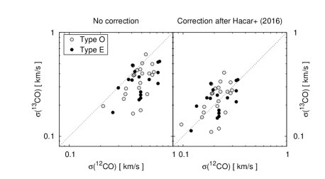
Figure 13: Comparison of the velocity dispersion measured in ¹²CO and ¹³CO for associated clumps. The left plot compares the directly measured line widths, the right plot shows the dispersions after the optical depth correction.

To measure the velocity dispersion of molecules from the line width of optically thick lines we have to apply an optical depth broadening following Hacar et al. (2016). Using the measured $X$-factors from in Sect. 5.1 we derive in Sect. 5.4.1 approximate correction factors of about 2.2 for the ¹²CO and about 1.4 for the ¹³CO clumps. Both factors are uncertain within about 10 % as the computation of the optical depth from the $X$-factors tends to underestimate the optical depth, due to the neglect of the change of the line shape, while the use of the relation for the thermal line width from Hacar et al. (2016), ignoring the small suprathermal contribution (see Sect. 5.4), tends to overestimate the correction. To verify the correction factors for the two linewidths we show in Fig. 13 the velocity dispersion measured in ¹²CO and ¹³CO for associated clumps that should see the same gas. Without the optical depth correction there is a clear offset from the identity line. After the correction both velocity dispersions match within a factor of two, symmetric to the identity line. This indicates that we obtain reliable estimates of the clump velocity dispersions.

References

- André et al. (2014) André, P., Di Francesco, J., Ward-Thompson, D., Inutsuka, S.-I., Pudritz, R., Pineda, J., 2014, in: Protostars and Planets VI, ed. H. Beuther, R. S. Klessen, C. Dullemond, T. Henning, pp. 27-52
- André et al. (2010) André, P., Men’shchikov, A., Bontemps, S., Könyves, V., Motte, F., Schneider, N., Didelon, P., Minier, V., et al., 2010, A&A, 518, L102
- Alves, Lombardi & Lada (2007) Alves, J., Lombardi, M., Lada, C., 2007, A&A, 462, L17
- Arshakian & Ossenkopf (2016) Arshakian, T. G.; Ossenkopf, V. 2016, A&A 585, 98
- Ballesteros-Paredes (2006) Ballesteros-Paredes, J., 2006, MNRAS, 372, 443
- Ballesteros-Paredes & MacLow (2002) Ballesteros-Paredes, J., Mac Low, M.-M., 2002, ApJ, 570, 734
- Beaumont et al. (2013) Beaumont, C., Offner, S., Shetty, R., Glover, S., Goodman, A., 2013, ApJ, 777, 173
- Bertoldi & McKee (1992) Bertoldi, F., McKee, C., 1992, ApJ, 395, 140
- Blake et al. (1987) Blake, G., Sutton, E., Masson, C., Phillips, T., 1987, ApJ, 315, 621
- Blitz & Thaddeus (1980) Blitz, L., Thaddeus, P., 1980, ApJ, 241, 676
- Bolatto, Wolfire & Leroy (2013) Bolatto, A., Wolfire, M., Leroy, A., 2013, ARA&A, 51, 207
- Cambrésy et al. (2013) Cambrésy, L., Marton, G., Feher, O., Tóth, L., Schneider, N., 2013, A&A, 557, 29
- Casseli & Myers (1995) Casseli, P., Myers, P., 1995, ApJ, 446, 665
- Clark, Klessen & Bonnell (2007) Clark, P., Klessen, R. S., Bonnell, I., 2007, MNRAS, 379, 57
- Clauset et al. (2009) Clauset, A., Shalizi, C. R., Newman, M. E. J., 2009, SIAM Rev., 51, No. 4, 661
- Csengeri et al. (2014) Csengeri, T., Urquhart, J., Schuller, F., Motte, F., Bontemps, S., Wyrowski, F., Menten, K., Bronfman, L., et al., 2014, A&A, 565, A75
- Curtis & Richer (2010) Curtis, E., & Richer, J., 2010, MNRAS, 402, 603
- Dame, Hartmann & Thaddeus (2001) Dame, T. M., Hartmann, D., & Thaddeus, P. 2001, ApJ, 547, 792
- Dent et al. (2009) Dent, W., Hovey, G., Dewdney, P., Burgess, T., Willis, A., Lightfoot, J., Jenness, T., Leech, J., et al., 2009, MNRAS, 395, 1805
- Dib et al. (2007) Dib, S.. Kim, J., Vázquez-Semadeni, E., Burkert, A., & Shadmehri, M., 2007, ApJ, 661, 262
- Di Francesco et al. (2010) Di Francesco, J., Sadavoy, S., Motte, F., Schneider, N., Hennemann, M., Csengeri, T., Bontemps, S., Balog, Z., et al., 2010, A&A, 518, L91
- Draine (2011) Draine, B., 2011, Physics of the Interstellar and Intergalactic Medium, Princeton University Press, ISBN: 978-0-691-12214-4
- Elmegreen (2002) Elmegreen, B., 2002, ApJ, 564, 773
- Elmegreen & Falgarone (1996) Elmegreen, B., Falgarone, E., 1996, ApJ, 471, 816
- Falgarone et al. (1992) Falgarone, E., Puget, J.-L., Pérault, M., 1992, A&A, 257, 715
- Frerking, Langer & Wilson (1982) Frerking, M., Langer, W., & Wilson, R., 1982, ApJ, 262, 590
- Gibson et al. (2009) Gibson, D. Plume, R., Bergin, E., Ragan, S., Evans, N., 2009, ApJ, 705, 123
- Glover & Mac Low (2011) Glover, S., Mac Low, M.-M., 2011, MNRAS, 412, 337
- Goodman et al. (1998) Goodman, A., Barranco, J., Wilner, D., Heyer, M., 1998, ApJ, 504, 223
- Hacar et al. (2016) Hacar, A.; Alves, J.; Burkert, A.; Goldsmith, P. 2016, A&A 591, 104
- Heithausen et al. (1998) Heithausen, A., Bensch, F., Stutzki, J., Falgarone, E., Panis, J., 1998, A&A, 331, 65
- Hennebelle & Falgarone (2012) Hennebelle, P., Falgarone, E, 2012, A&ARv, 20, 55
- Hennemann et al. (2010) Hennemann, M., Motte, F., Bontemps, S., Schneider, N., Csengeri, T., Balog, Z., di Francesco, J., Zavagno, A., et al., 2010, A&A, 518, L84
- Heyer & Brunt (2004) Heyer, M., Brunt, C., 2004, ApJ, 615, L45
- Heyer et al. (2009) Heyer, M., Krawczyk, C., Duval, J., Jackson, J., 2009, ApJ, 699, 1092
- Heyer, Williams & Brunt (2006) Heyer, M., Williams, J., Brunt, C., 2006, ApJ, 643, 956
- Hill et al. (2011) Hill, T., Motte, F., Didelon, P., Bontemps, S., Minier, V., Hennemann, M., Schneider, N., André, Ph., et al., 2011, A&A, 533, 94
- Hughes & Chraibi (2012) Hughes, G., Chraibi, M., 2012, Computing and Visualization in Science, Vol. 15, Issue 5, 291
- Ibáñez-Mejía et al. (2016) Ibáñez-Mejía, J., Mac Low, M.-M., Klessen, R. S., Baczynski, C., 2016, ApJ, 824, 41
- Juvela et al. (2015) Juvela, M.; Ristorcelli, I.; Marshall, D. J.; et al. 2015, A&A, 584, 93
- Kauffmann et al. (2010a) Kauffmann, J., Pillai, T., Shetty, R., Myers, P., Goodman, A., 2010a, ApJ, 712, 1137
- Kauffmann et al. (2010b) Kauffmann, J., Pillai, T., Shetty, R., Myers, P., Goodman, A., 2010b, ApJ, 716, 433
- Kauffmann, Pillai & Goldsmith (2013) Kauffmann, J., Pillai, T., Goldsmith, P., 2013, 779, 185
- Klessen & Glover (2015) Klessen, R. S., Glover, S., 2015, in Star Formation in Galaxy Evolution: Connecting Numerical Models to Reality, Saas-Fee Advanced Course, Vol. 43, pp. 85-249, Springer, ISBN: 978-3-662-47889-9
- Kolmogorov (1941) Kolmogorov, A., 1941, Dokl. Akad. Nauk SSSR, 30, 301
- Kramer et al. (1998) Kramer, C., Stutzki, J., Rohrig, R., Corneliussen, U., 1998, A&A, 329, 249
- Larson (1981) Larson, R., 1981, MNRAS, 194, 809
- Lombardi, Alves & Lada (2010) Lombardi, M., Alves, J., Lada, C., 2010, A&A, 519, 7
- Lombardi, Alves & Lada (2011) Lombardi, M., Alves, J., & Lada, C., 2011, A&A, 535, A16
- Mangum & Shirley (2015) Mangum, J., Shirley, Y., 2015, PASP, 127, 266
- McKee & Zweibel (1992) McKee, C. , & Zweibel, E., 1992, ApJ, 399, 551
- Men’shchikov et al. (2012) Men’shchikov, A., André, P., Didelon, P., Motte, F., Hennemann, M., Schneider, N., 2012, A&A, 542, 81
- Motte, Schilke & Lis (2003) Motte, F., Schilke, P., Lis, D., 2003, ApJ, 582, 277
- Motte et al. (2010) Motte, F., Zavagno, A., Bontemps, S., Schneider, N., Hennemann, M., Di Francesco, J., André, Ph., Saraceno, P., et al., 2010, A&A, 518, L77
- Myers & Goodman (1988) Myers, P., Goodman, A., 1988, ApJ, 326, L27
- Nagahama et al. (1998) Nagahama, T., Mizuno, A., Ogawa, H., & Fukui, Y. 1998, AJ, 116, 336
- Ossenkopf & Henning (1994) Ossenkopf, V., Henning, T., 1994, A&A, 291, 943
- Ossenkopf (2002) Ossenkopf, V., 2002, A&A, 391, 295
- Pekruhl et al. (2013) Pekruhl, S., Preibisch, T., Schuller, F., Menten, K., 2013, A&A, 550, A29
- Phelps & Lada (1997) Phelps R. L., Lada E. A., 1997, ApJ, 477, 176
- Phillips et al. (1979) Phillips, T. G., Huggins, P. J., Wannier, P. G., & Scoville, N. Z. 1979, ApJ, 231, 720
- Poulton et al. (2008) Poulton, C.J.; Robitaille, T.B.; Greaves, J.S.; et al.; 2008, MNRAS, 384, 1249
- Reid et al. (2010) Reid, M., Wadsley, J., Petitclerc, N., Sills, A., 2010, ApJ, 719, 561
- Román-Zúñiga & Lada (2008) Román-Zúñiga, C., Lada, E., 2008, in: Handbook of Star Forming Regions, Vol. I: The Northern Sky ASP Monograph Publications, Vol. 4, Bo Reipurth, ed., p.928
- Rosolowsky et al. (2008) Rosolowsky, E., Pineda, J., Kauffmann, J., Goodman, A., 2008, ApJ, 679, 1338
- Roy et al. (2013) Roy, A., Martin, P., Polychroni, D., Bontemps, S., Abergel, A., André, Ph., Arzoumanian, D., Di Francesco, J., et al., 2013, ApJ, 763, 55
- Russeil et al. (2013) Russeil, D., Schneider, N., Anderson, L., Zavagno, A., Molinari, S., Persi, P., Bontemps, S., Motte, F., et al., 2013, A&A, 554, 42
- Salpeter (1955) Salpeter, E., 1955, ApJ, 121, 161
- Schneider & Brooks (2004) Schneider, N., Brooks, K., 2004, PASA, 21, 290
- Schneider et al. (2016) Schneider, N.; Bontemps, S.; Motte, F.; et al., 2016, A&A, 587, 74
- Schneider et al. (2012) Schneider, N., Csengeri, T., Hennemann, M., Motte, F., Didelon, P., Federrath, C., Bontemps, S., Di Francesco, J., et al., 2012, A&A, 540, L11
- Schneider et al. (2010) Schneider, N., Motte, F., Bontemps, S., Hennemann, M., di Francesco, J., André, Ph., Zavagno, A., Csengeri, T., et al., 2010, A&A, 518, L83
- Schneider et al. (1998) Schneider, N., Stutzki, J., Winnewisser, G., Block, D., 1998, 335, 1049
- Shetty et al. (2010) Shetty, R., Collins, D., Kauffmann, J., Goodman, A., Rosolowsky, E., & Norman, M., 2010, ApJ, 712, 1049
- Shetty et al. (2011) Shetty, R., Glover, S., Dullemond, C., Klessen, R., 2011, MNRAS, 412, 1686
- Shirley et al. (2003) Shirley, Y., Evans, N., II, Young, K., Knez, C., Jaffe, D., 2003, ApJS, 149, 375
- Solomon et al. (1987) Solomon, P., Rivolo, A., Barrett, J., Yahil, A., 1987, ApJ, 319, 730
- Stutzki & Güsten (1990) Stutzki, J., & Güsten, R., 1990, ApJ, 356, 513
- Szűcs, Glover & Klessen (2016) Szűcs, L., Glover, S., Klessen, R. S., 2016, MNRAS, 460, 82
- Veltchev, Donkov & Klessen (2013) Veltchev, T., Donkov, S., Klessen, R. S., 2013, MNRAS, 432, 3495
- Williams, Blitz & Stark (1995) Williams, J., Blitz, L., Stark, A., 1995, ApJ, 451, 252
- Williams, de Geus & Blitz (1994) Williams, J., de Geus, E., Blitz, L., 1994, ApJ, 428, 693
- Wu et al. (2010) Wu, J., Evans, N., Shirley, Y., Knez, C., 2010, ApJS, 188, 313
- Zhang, Xu & Yang (2014) Zhang, S., Xu, Y., & Yang, J., 2014, AJ, 147, 46