Anomalous magnon Nernst effect of topological magnonic materials

Abstract

The magnon transport driven by thermal gradient in a perpendicularly magnetized honeycomb lattice is studied. The system with the nearest-neighbor pseudodipolar interaction and the next-nearest-neighbor Dzyaloshinskii-Moriya interaction (DMI) has various topologically nontrivial phases. When an in-plane thermal gradient is applied, a transverse in-plane magnon current is generated. This phenomenon is termed as the anomalous magnon Nernst effect that closely resembles the anomalous Nernst effect for an electronic system. The anomalous magnon Nernst coefficient and its sign are determined by the magnon Berry curvatures distribution in the momentum space and magnon populations in the magnon bands. We predict a temperature-induced sign reversal in anomalous magnon Nernst effect under certain conditions.

I Introduction

Spintronics is about generation, detection and manipulation of spin degree of freedom of particles. Most early studies focused on the electron spins DasSarma . However, an electric current normally accompanies an electron spin current and consumes much energy, leading to a Joule heating. The Joule heating becomes the critical problem in nano electronics and spintronics although many efforts have been made. Recently, magnon spintronics, or magnonics in which magnons are spin carriers, attracts much attention because of its fundamental interest xiansi ; hubin and its lower energy consumption in comparison with that of electron spintronics book1 ; magnonics1 ; magnonics2 .

Nernst effect commonly refers to the generation of a transverse voltage/current by a thermal gradient in an electronic system under a perpendicular magnetic field. In a ferromagnetic metal and in the absence of an external magnetic field, a thermal gradient can generate a transverse charge current or voltage proportional to the vector product of the thermal gradient and the magnetization in the linear response region. This is the anomalous Nernst effect, the thermal electric manifestation of the anomalous Hall effect ANE . It is natural to ask whether there is a similar effect for magnons. Moving magnons experience gyroscopic forces because of nonzero Berry curvature of a magnetic system although magnons are charge neutral quasiparticles that do not have the Lorentz force. As a result, a transverse magnon current is generated when magnons are driven by a longitudinal force such as a thermal gradient in the absence of a magnetic field which is termed as the anomalous magnon Nernst effect (AMNE). In this paper, we focus on a perpendicularly magnetized honeycomb lattice with the nearest-neighbor pseudodipolar interaction and the next-nearest-neighbor Dzyaloshinskii-Moriya interaction (DMI), whose magnon bands can be topologically nontrivial with various topological phases ours . We investigate the magnon transport of this system in the presence of a thermal gradient using the semiclassical equations of motion of magnons and the Boltzmann equation in linear transport regime. We found that the system has topologically nontrivial magnon bands. The system changes from one topologically nontrivial phase to another as the DMI strength varies. The AMNE coefficient depends on temperature nonmonotonically. It starts from 0 at 0 K and goes back to 0 at high temperature limit with a maximum at an intermediate temperature. The nonmonotonical temperature-dependence of AMNE is due to non-trivial Berry curvature distribution of a given band in the momentum space and thermally activated magnon population in the bands. In certain parameter space, there is a sign reversal of the AMNE at low temperature because the magnon Berry curvature near the band bottom at $\Gamma$ point has small non-zero values of the opposite sign as those near band top at K and K^′ points with a much bigger value. In the presence of staggered anisotropy on A, B sublattices, the system can also be topologically trivial, and the K and K^′ valleys contribute opposite transverse magnon currents due to the opposite Berry curvatures. However, the total transverse magnon current does not vanish. The boundary that AMNE coefficient changes its sign is also determined numerically.

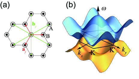
Figure 1: (a) Schematic illustration of a perpendicularly magnetized honeycomb lattice. The red and green arrows denote the nearest-neighbor and the next-nearest-neighbor vectors, respectively. (b) Magnon spectrum $\omega(\mathbf{k})$ of an infinite system for $K=10J$, $F=5J$, and $D=\Delta=0$. The Brillouin zone is indicated by the black hexagon.

II Model and Results

We consider classical magnetic moments on a honeycomb lattice in the $xy$ plane as illustrated in Figure 1(a), and the Hamiltonian is

$$\mathcal{H}=-\frac{J}{2}\sum_{\left\langle i,j\right\rangle}\mathbf{m}_{i}\cdot\mathbf{m}_{j}-\frac{F}{2}\sum_{\left\langle i,j\right\rangle}(\mathbf{m}_{i}\cdot\mathbf{e}_{ij})(\mathbf{m}_{j}\cdot\mathbf{e}_{ij})-D\sum_{\langle\langle i,j\rangle\rangle}\nu_{ij}\hat{\mathbf{z}}\cdot\left(\mathbf{m}_{i}\times\mathbf{m}_{j}\right)-\sum_{i}\frac{K_{i}}{2}m_{iz}^{2},$$ (1)

where the first term is the nearest-neighbor ferromagnetic Heisenberg exchange interaction ($J>0$). The second and third terms arise from the spin-orbit coupling (SOC) pseudo ; DMI . $\mathbf{e}_{ij}$ is the unit vector pointing from site $i$ to $j$. $F$ is the strength of the nearest-neighbor pseudodipolar interaction, which is the second-order effect of the SOC [The nearest-neighbor Dzyaloshinskii-Moriya interaction (DMI) would be the first-order effect of SOC if it exists, but it vanishes because the center of the A-B bond is an inversion center of the honeycomb lattice]. The next-nearest-neighbor DMI measured by $D$ is in general no zero. $\nu_{ij}=\frac{2}{\sqrt{3}}\hat{\mathbf{z}}\cdot(\mathbf{e}_{li}\times\mathbf{e}_{lj})=\pm 1$, where $l$ is the nearest neighbor site of $i$ and $j$. The last term is the sublattice-dependent anisotropy whose easy-axis is along the $z$ direction with anisotropy coefficients of $K_{i}=K+\Delta$ for $i\in$ A and $K-\Delta$ for $i\in$ B. $\mathbf{m}_{i}$ is the unit vector of the magnetic moment at site $i$. The spin dynamics is governed by the Landau-Lifshitz-Gilbert (LLG) equation LLG ; ours ,

$$\frac{\mathrm{d}\mathbf{m}_{i}}{\mathrm{d}t}=-\gamma\mathbf{m}\times\mathbf{H}^{\text{eff}}_{i}+\alpha\mathbf{m}_{i}\times\frac{\mathrm{d}\mathbf{m}_{i}}{\mathrm{d}t},$$ (2)

where $\gamma$ is the gyromagnetic ratio and $\alpha$ is the Gilbert damping constant. $\mathbf{H}^{\text{eff}}_{i}=\frac{\partial\mathcal{H}}{\mu_{0}\mu\partial\mathbf{m}_{i}}$ is the effective field at site $i$. The lattice constant $a$ and $J$ are used as the length unit and the energy unit out of five parameters in (1). The magnetic field and time are in the units of $\sqrt{J\mu_{0}/a^{3}}$ and $\sqrt{a^{3}\mu_{0}/(J\gamma^{2})}$, respectively, where $\mu_{0}$ is the vacuum permeability. When the anisotropy is sufficiently large, spins are perpendicularly magnetized split . To obtain the spin wave spectrum, we linearize the LLG equation following the standard procedures ours . The spin wave spectrum and wavefunctions are obtained by solving the eigenvalue problem $gH(\mathbf{k})\psi_{n}=\omega_{n}(\mathbf{k})\psi_{n}$, where $H(\mathbf{k})$ is a $4\times 4$ Hermitian matrix

$$H=\left(\begin{matrix}M_{\mathrm{A}}^{+}&0&-\ell(\mathbf{k})&-g_{+}(\mathbf{k})\\ 0&M_{\mathrm{A}}^{-}&-g_{-}(\mathbf{k})&-\ell(\mathbf{k})\\ -\ell^{*}(\mathbf{k})&g_{-}^{*}(\mathbf{k})&M_{\mathrm{B}}^{-}&0\\ -g_{+}^{*}(\mathbf{k})&\ell^{*}(\mathbf{k})&0&M_{\mathrm{B}}^{+}\end{matrix}\right),$$ (3)

with $\ell(\mathbf{k})=\left(J+\frac{F}{2}\right)\sum_{j=1,2,3}e^{i\mathbf{k}\cdot\mathbf{a}_{j}}$, $g_{\pm}(\mathbf{k})=\frac{F}{2}\sum_{j=1,2,3}e^{\pm 2i\theta{j}}e^{i\mathbf{k}\cdot\mathbf{a}_{j}}$ ($\theta_{j}$ is the angle between $\mathbf{a}_{j}$ and $x$ direction). $M_{\mathrm{A}}^{\pm}=M+\Delta\pm d(\mathbf{k})$ and $M_{\mathrm{B}}^{\pm}=M-\Delta\pm d(\mathbf{k})$ with $M=K+3J$ and $d(\mathbf{k})=2D\sum_{j=1,3,5}\sin(\mathbf{k}\cdot\mathbf{b}_{j})$. $g=\sigma_{0}\bigotimes\sigma_{3}$ (with $\sigma_{0}$ being the $2\times 2$ identity matrix and $\sigma_{3}$ the Pauli matrix). $\psi_{n}$ is the $n$th eigenvector of eigen-frequency $\omega_{n}$, satisfying the generalized orthogonality $\psi_{i}^{\dagger}g\psi_{j}=\delta_{ij}$. At K and K^′, the frequencies of the two magnon bands are respectively,

$$\omega_{1}^{\mathrm{K(K^{\prime})}}=M-3\sqrt{3}D+(-)\Delta,$$ (4)

$$\omega_{2}^{\mathrm{K(K^{\prime})}}=\sqrt{(M+3\sqrt{3}D)^{2}-\frac{9}{4}F^{2}}-(+)\Delta,$$ (5)

where “$(+)$” and “$(-)$” on the right hand side are for K^′. The magnon band for $K=10J$, $F=5J$ and $D=\Delta=0$ is shown in Figure 1(b), which has a direct gap of $\Delta_{g}=M-\sqrt{M^{2}-9F^{2}/4}$ at both K and K^′ (valleys for the upper band and peaks for the lower band). The direct gap at the valleys can close and reopen as $D$ and $\Delta$ varies, resulting in topological phase transitions. The Berry curvature $\boldsymbol{\Omega}_{n}$ of $n$th band and the corresponding Chern number $\mathcal{C}_{n}$ can be calculated by using a gauge-invariant formula Shindou ,

$$\boldsymbol{\Omega}_{n}=i\nabla_{\mathbf{k}}\times\left(\psi_{n}^{\dagger}g\nabla_{\mathbf{k}}\psi_{n}\right);$$ (6)

$$\mathcal{C}_{n}=\frac{1}{2\pi}\iint_{\mathbf{k}\in\mathrm{BZ}}\Omega_{n}d^{2}\mathbf{k},$$ (7)

where the integration is over the Brillouin zone (BZ), and $\Omega_{n}=\boldsymbol{\Omega}_{n}\cdot\hat{\mathbf{z}}$ is the $z$ component of the Berry curvature that is given by a gauge-invariant formula similar to that in electronic systems chern

$$\boldsymbol{\Omega}_{n}=i\mathrm{Tr}\left[P_{n}\left(\frac{\partial P_{n}}{\partial k_{x}}\frac{\partial P_{n}}{\partial k_{y}}-\frac{\partial P_{n}}{\partial k_{y}}\frac{\partial P_{n}}{\partial k_{x}}\right)\right]\hat{\mathbf{z}},$$ (8)

where $P_{n}$ is the projection matrix of the $n$th band defined as $P_{n}=\psi_{n}\psi_{n}^{\dagger}g$.

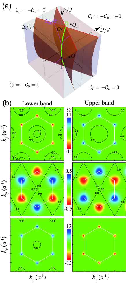
Figure 2: (a) Phase diagram in $D/J-\Delta/J-F/J$ space for $K=10J$. Phases are classified by the Chern numbers of the upper and lower magnon bands. Three phases of $C_{l}=-C_{u}=1$; $C_{l}=-C_{u}=-1$; and $C_{l}=C_{u}=0$ are separated by two orange boundary surfaces. The green line, $D=\frac{\sqrt{3}F^{2}}{16M}$ and $\Delta=0$, is the intersection of the two boundary surfaces. The magenta lines, $\Delta=\pm\Delta_{g}/2$ and $D=0$, are the intersections of the boundary surfaces with the $D=0$ plane. $O_{1}$ ($F=5J$, $D=\Delta=0$), $O_{2}$ ($F=5J$, $D=0.4J$, $\Delta=0$), and $O$ ($F=D=0$, $\Delta=-1.5J$) are 3 representative points in topologically nontrivial phase of $C_{l}=-C_{u}=-1$; $C_{l}=-C_{u}=1$, and topologically trivial phase $C_{l}=C_{u}=0$, respectively. (b) The $z$ component of Berry curvature $\Omega=\boldsymbol{\Omega}\cdot\hat{\mathbf{z}}$ for $O_{1}$, $O$, $O_{2}$ (from top to bottom). The left panel is for the lower magnon band and the right panel for the upper magnon band. The color bars are shown at the middle. The contour line of $\Omega=0$ is shown by the dashed circles. The white hexagons is the fisrt Brillouin zone.

Figure 2(a) is the phase diagram in $D/J-\Delta/J-F/J$ space for $K=10J$. The various topological phases are classified by Chern numbers $\mathcal{C}_{l}$ and $\mathcal{C}_{u}$ of lower and upper magnon bands. $\mathcal{C}_{l}+\mathcal{C}_{u}=0$ satisfies the “zero sum rule” chern ; book_niu . The magnon band Chern number change its value when magnon band gap closes and reopens at valley K or K^′. Thus, the band gap closing at K or K^′ defines two phase boundary surfaces of $\omega_{1}^{K\prime}=\omega_{2}^{K\prime}$ and $\omega_{1}^{K}=\omega_{2}^{K}$ (See Eqs. (4) and (5)). For convenience, we define

$$\Delta_{c}=\frac{1}{2}\left[\sqrt{(M+3\sqrt{3}D)^{2}-\frac{9}{4}F^{2}}-(M-3\sqrt{3}D)\right],$$ (9)

and two phase boundary surfaces are $\Delta=\pm\Delta_{c}$, denoted as the orange surfaces. They divide the whole space into four regions. In the region of $\Delta_{c}<0$ and $\Delta_{c}<\Delta<-\Delta_{c}$, $C_{u}$ is $1$. The density plot of $\Omega$ for $F=5J$, $\Delta=D=0$ ($O_{1}$ in Fig. 2(a)) is shown in the top panel of Fig. 2(b). Interestingly, the lower band has two contour curves of $\Omega=\Omega_{l}=0$ around $\Gamma$ denoted by black dash lines. The two contour curves divide the first Brillouin zone into three parts. $\Omega$ is slightly positive inside the inner contour curve around $\Gamma$ for the lower band as shown in the top left panel. Between two contour curves, $\Omega$ is slightly negative. $\Omega$ is positive outside the outer contour curve as shown in the top left panel of Fig. 2(b), but significant non-zero $\Omega$ occurs only around K and K^′. In the region of $\Delta_{c}>0$ and $-\Delta_{c}<\Delta<\Delta_{c}$, the upper magnon band has Chern number $-1$. The bottom panel of Fig. 2(b) is the density plot of $\Omega$ of lower (left panel) and upper (right panel) bands for a representative point of $F=5J$, $\Delta=0$, $D=0.4J$ ($O_{2}$ in Fig. 2(a)) in this topologically nontrivial phase. The lower band has only one contour curve of $\Omega=0$ (black dash curve) around $\Gamma$ that divides the first Brillouin zone into two parts. Inside the contour curve, $\Omega$ is slightly positive as shown in the bottom left panel of Fig. 2(b). It is negative outside the contour curve with significant non-zero value around K and K^′. The system is in topologically trivial phase for both lower and upper bands in the other two regions. $\Omega$ around K and K^′ valleys have opposite sign so that the Chern numbers are 0 for both bands. We consider $O$ in Fig. 2(a) ($F=D=0$, $\Delta=1.5J$) as a representative point in the phase. The middle panel of Fig. 2(b) shows the density plot of $\Omega$ at $O$ for the two bands. Indeed, Berry curvatures $\Omega$ at K and K^′ have opposite value, and Chern numbers are zeros. For $\Delta=0$, the band gaps at K and K^′ close and reopen at the same time and the Chern number of the upper band changes from $-1$ to $+1$ if we tune the DMI crossing the line of $D=\frac{\sqrt{3}F^{2}}{16M}$ and $\Delta=0$ [the green line in Figure 2(a)]. The system changes from one topologically nontrivial phase to another. The features of the phase diagram discussed above preserves as long as system ground state is the perpendicular ferromagnetic state.

Let us consider the magnon transport in an infinite system. Apply a thermal gradient along $x$ direction, the motion of a magnon wavepacket is governed by the semiclassical equations Niu ; Murakami ,

$$\dot{\mathbf{r}}=\frac{1}{\hbar}\frac{\partial\varepsilon}{\partial\mathbf{k}}-\dot{\mathbf{k}}\times\boldsymbol{\Omega};$$ (10)

$$\dot{\mathbf{k}}=\frac{1}{\hbar}\mathbf{F}=-\frac{1}{\hbar}\frac{\partial\varepsilon}{\partial\mathbf{r}}+\frac{q}{\hbar}\dot{\mathbf{r}}\times\mathbf{B},$$ (11)

Where $\varepsilon(\mathbf{r},\mathbf{k})=\hbar\omega(\mathbf{k})+\phi(\mathbf{r})$ is the energy of the magnon with $\phi(\mathbf{r})$ being the potential energy, and $\mathbf{F}$ is the total force on the magnon. $q$ is the charge of the particle and $q=0$ for a magnon. In the presence of a thermal gradient, the Boltzmann equation of the magnon is

$$\dot{\mathbf{r}}\cdot\frac{\partial f}{\partial\mathbf{r}}=-\frac{f-f_{0}}{\tau}\equiv-\frac{f_{1}}{\tau},$$ (12)

where $f(\mathbf{r},\mathbf{k})$ is the magnon distribution function. $f_{0}=1/(e^{\beta\hbar\omega}-1)$ is the Bose-Einstein distribution of zero chemical potential at local temperature $T$ [$\beta=(k_{B}T)^{-1}$]. $\tau$ is magnon relaxation time. $f_{1}$ is the deviation of the distribution function from its equilibrium values. In the linear response regime where the thermal gradient is small, Eq. (12) can be written as

$$\dot{\mathbf{r}}\cdot\frac{\partial f_{0}}{\partial\mathbf{r}}=-\frac{f_{1}}{\tau}.$$ (13)

One can prove the following identity,

$$\dot{\mathbf{r}}\cdot\frac{\partial f_{0}}{\partial\mathbf{r}}=\left(-\frac{\hbar\omega}{T}\nabla T\right)\cdot\frac{\partial f_{0}}{\hbar\partial\mathbf{k}}.$$ (14)

Substituting Eq. (14) into the left hand side of Eq. (13), it yields

$$\left(-\frac{\hbar\omega}{T}\nabla T\right)\cdot\frac{\partial f_{0}}{\hbar\partial\mathbf{k}}=-\frac{f_{1}}{\tau}.$$ (15)

Thus, one can identify a thermal force $\mathbf{F}_{T}=\left(-\frac{\hbar\omega}{T}\nabla T\right)$ proportional to the magnon frequency and the thermal gradient thermalforce . Insert (11) into (10) with $\mathbf{F}=\mathbf{F}_{T}$, we obtain

$$\dot{\mathbf{r}}=\frac{\partial\omega}{\partial\mathbf{k}}+\frac{\omega}{T}\nabla T\times\boldsymbol{\Omega}.$$ (16)

The magnon current density is given by $\mathbf{j}_{m}=\sum_{n,\mathbf{k}}\left[\dot{\mathbf{r}}f(n,\mathbf{k})\right]$, where the summation is over all magnon states. Keep terms linear in the thermal gradient and convert the summation to integration, we have

$$\mathbf{j}_{m}=\tensor{\boldsymbol{\kappa}}(-k_{B}\nabla T),$$ (17)

where the longitudinal heat conductance $\kappa_{xx}$ and the anomalous Nernst coefficient $\kappa_{xy}$ are

$$\kappa_{xx}=\frac{\tau}{(2\pi)^{2}}\sum_{n}\iint\beta\left(\frac{\partial\omega_{n}}{\partial k_{x}}\right)^{2}\rho\left(\beta\hbar\omega_{n}\right)d^{2}\mathbf{k},$$ (18)

$$\kappa_{xy}=\frac{1}{(2\pi)^{2}}\sum_{n}\iint\beta\omega_{n}\Omega_{n}f_{0}\left(\beta\hbar\omega_{n}\right)d^{2}\mathbf{k},$$ (19)

where $\rho(x)=\frac{xe^{x}}{(e^{x}-1)^{2}}$, $f_{0}(x)=\frac{1}{e^{x}-1}$, and $n=1,2$ labels the lower and upper magnon bands. Figure 3(a) shows the temperature dependence of $\kappa_{xx}$ and $\kappa_{xy}$ in two different topologically-nontrivial phases specified by $O_{1}$ and $O_{2}$ in Fig. 2(a). In order to have a quantitative feeling about the results, we use $\mathrm{Sr_{2}IrO_{4}}$ parameters of $a=0.55$ nm para , $J=19.6\mu_{0}\mu_{B}^{2}/a^{3}$ pseudo , and $\gamma=2.21\times 10^{5}$ rad/s/(A/m) in all the following discussions. The longitudinal heat conductance $\kappa_{xx}$ is always positive as expected from thermodynamic laws that the magnons move from the hot side to the cold side. Eq. (19) says that the AMNE coefficient is determined by the Berry curvature distribution in the momentum space and the magnon equilibrium distribution function. Since magnon number in the lower band is bigger than that in the higher band according to the Bose-Einstein distribution, the sign of AMNE coefficient is always determined by the Berry curvature of the lower magnon band. At very low temperature, only the magnons near$\Gamma$ point [band bottom (top) of the lower (upper) band) are excited. The sign of AMNE coefficient is determined by $\Omega$ around $\Gamma$, and its value is small because Berry curvature $\Omega$ is very close to zero, if not exactly zero, and the magnon number is also small there. At a higher temperature when the magnon number near K and K^′ points [band top (bottom) of the lower (lower) band] are large enough and dominate the AMNE due to significant non-zero values of the Berry curvature only near there. At even higher temperature when equal-partition theorem become true so that $f_{0}\approx k_{B}T/(\hbar\omega)$, the AMNE coefficient is close to zero because $\kappa_{xy}$ is approximately proportional to $(\mathcal{C}_{u}+\mathcal{C}_{l})=0$ chern ; book_niu , i.e. the contributions from two bands cancel with each other.

The general behavior of AMNE coefficient $\kappa_{xy}$ mentioned above can be illustrated by two representative points in two distinct topologically nontrivial phases of $C_{l}=-1$ (for $O_{1}$) and $C_{l}=1$ (for $O_{2}$). For $O_{1}$ whose Berry curvature distribution is given in the top panel of Fig. 2(b), $\kappa_{xy}$ is always positive, a transverse magnon current along $\mathbf{m}_{0}\times(-\nabla T)$, because $\Omega$ are positive near both $\Gamma$ and K ($K^{\prime}$) points. For $O_{2}$, at very low temperatures when the magnon number around K and K^′ are negligible and only the magnons near $\Gamma$ point are excited, $\kappa_{xy}$ decreases and becomes more and more negative initially with the increase of temperature because $\Omega$ is negative near $\Gamma$ point. However, when magnons near K and K^′ points are excited, $\kappa_{xy}$ starts to increase with temperature, and becomes postive after an intermediate temperature because $\Omega$ has large positive values near K and K^′. Thus, in this phase the sign of the AMNE coefficient reverses at the intermediate temperature. The numerical results of $\kappa_{xx}$ and $\kappa_{xy}$ at higher temperature are shown in the inset of Figure 3(a). The longitudinal heat conductance $\kappa_{xx}$ saturates at high temperature. AMNE coefficient $\kappa_{xy}$ at $O_{1}$ ($O_{2}$) increases from 0 to a maximum positive (negative) value as the temperature increases, and then gradually go back to 0 when magnons in the upper band are thermally excited. This indicates that there is an optimal temperature for the maximal AMNE coefficient. If this temperature does not exceed the Curie temperature, it should be used for the largest AMNE.

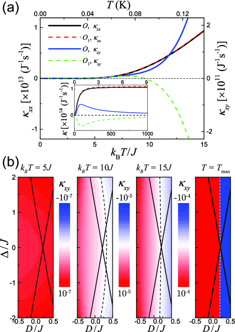
Figure 3: (a) The longitudinal magnon conductance $\kappa_{xx}$ (left axis) and AMNE coefficient $\kappa_{xy}$ (right axis) for parameters at $O_{1}$ and $O_{2}$. The inset shows the high-temperature values of the same quantities. (b) (Panels 1 to 3) The density plots of $\kappa_{xy}$ [in units of $\mathrm{eV^{-1}s^{-1}}$] in $D/J$- $\Delta/J$ plane for $K=10J$ and $F=5J$ at different temperatures. The black solid lines are topological phase boundaries, and the black dashed lines are the contour lines of $\kappa_{xy}=0$. WHY COLOR BARS are negative on top and po on bot.? What are the use of black lines? (Panel 4) The sign of the maximum value of $\kappa_{xy}$. Red region is for positive $\kappa_{xy}$ and blue region is for negative $\kappa_{xy}$. The dashed line is the contour curve of $\kappa_{xy}=0$.

In the topologically trivial phase, the Berry curvatures $\Omega$ Of the same band has opposite values near K and K^′ points. Thus the contributions to AMNE from different valleys cancel each other, and the net transverse magnon current can be in either direction, depending on the parameters. Figure 3(b) is the density plots of $\kappa_{xy}$ as a function of $D/J$ and $\Delta/J$ at different temperatures (for $K=10J$ and $F=5J$). Because of the featured distribution of Berry curvature near $\Gamma$ discussed above, the sign change of $\kappa_{xy}$ happens at larger $D$ at lower temperatures, and is different to the topological phase boundaries as shown by the black solid lines. However, the sign change of $\kappa_{xy}$ is closely related to the topological phase transition, as shown in the last panel of Figure 3(b). The sign change of $\kappa_{xy}$ coincides with the topological phase transition line of $D=\frac{\sqrt{3}F^{2}}{16M}$ and $\Delta=0$. Tuning the DMI can drive the system from one topologically nontrivial phase to another at $\Delta=0$. The sign change of $\kappa_{xy}$ at the maximum point changes at the same time due to the sign-reversal of Berry curvatures. This also means for the parameters of negative $\kappa_{xy}$ in the last panel, there is a temperature-induced sign reversal of $\kappa_{xy}$.

In the above discussions, we studied the magnon Nernst effect, a transverse magnon current generated by a longitudinal thermal gradient. Similar to electronic systems, there are other related effects, such as a transverse magnon current induced by a longitudinal chemical potential gradient (magnon Hall effect and anomalous magnon Hall effect), and a transverse magnon heat current induced by a longitudinal chemical potential gradient (magnon Peltier effect). These effects can be investigated in the same way as what have done here for the same Berry curvature physics. Similar topological phase transitions and sign-reversal of AMNE was also predicted in pyrochlore lattices mook . In the calculation of thermal transport coefficients, the thermal energy $k_{B}T$ is allowed to be much higher than $J$. In real materials, the temperature is limited by the Curie temperature that is order of $J/k_{B}$. For example, $J=20$ meV ($2.5\times 10^{5}\mu_{0}\mu^{2}/a^{3}$) and the Curie temperature is about 240 K exp2012 for $\mathrm{Sr_{2}IrO_{4}}$. The sign-reversal temperature is $9.5J/k_{B}$ as shown in Figure 3(a). Thus, the temperature is much smaller than the sign-reversal temperature in this case so the AMNE coefficient should be always positive. The reason why the Berry curvature near $\Gamma$ point has opposite sign, and the factors that affect the Berry curvature distribution are still open questions.

III Conclusion

In conclusion, we studied the thermal magnon transport of perpendicularly magnetized honeycomb lattice with the nearest-neighbor pseudodipolar interaction and the next-nearest-neighbor DMI. We show that the system has various topological nontrivial phases. Due to the nontrivial Berry curvature, a transverse magnon current appears when a thermal gradient is applied, resulting in an anomalous Magnon Nernst effect. The sign of the anomalous Magnon Nernst effect is reversed by tuning DMI and temperature.

Reference

References

- (1) Z̆utić I, Fabian J and Das Sarma S 2004 Rev. Mod. Phys. 76 323
- (2) Wang X S, Yan P, Shen Y H, Bauer G E W and Wang X R 2012 Phys. Rev. Lett. 109 167209
- (3) Hu B and Wang X R 2013 Phys. Rev. Lett. 111 027205
- (4) Demokritov S O and Slavin A N 2013 Magnonics: From Fundamentals to Applications (Springer, Topics in Applied Physics Vol. 125)
- (5) Kruglyak V V , Demokritov S O and Grundler D 2010 J. Phys. D: Appl. Phys. 43 264001
- (6) Serga A A, Chumak A V and Hillebrands B 2010 J. Phys. D: Appl. Phys. 43 264002
- (7) Nagaosa N, Sinova J, Onoda S, MacDonald A H and Ong N P 2010 Rev. Mod. Phys. 82 1539
- (8) Wang X S, Su Y and Wang X R 2017 Phys. Rev. B 95 014435
- (9) Moriya T 1960 Phys. Rev. 120 91
- (10) Jackeli G and Khaliullin G 2009 Phys. Rev. Lett. 102 017205
- (11) Matsumoto R and Murakami S 2011 Phys. Rev. Lett. 106 197202
- (12) Gilbert T L 2004 IEEE. Trans. Magn. 40 3443
- (13) Wang X S, Zhang H W and Wang X R arXiv:1706.09548
- (14) White R M, Sparks M and Ortenburger I 1965 Phys. Rev. 139, A450
- (15) Avron J E, Seiler R and Simon B 1983 Phys. Rev. Lett. 51, 51
- (16) Shindou R, Matsumoto R, Murakami S and Ohe J I 2013 Phys. Rev. B 87 174427
- (17) Bohm A, Mostafazadeh A, Koizumi H, Niu Q and Zwanziger J 2003 The Geometric Phase in Quantum Systems: Foundations, Mathermatical Concepts, and Applications in Molecular and Condensed Matter Physics (Springer, Berlin).
- (18) Xiao D, Chang M -C and Niu Q 2010 Rev. Mod. Phys. 82 1959
- (19) Luttinger J M 1964 Phys. Rev. 135 A1505
- (20) Huang Q, Soubeyroux J L, Chmaissem O, Natali Sora I, Santoro A, Cava R J, Krajewski J J and Peck W F Jr 1994 J. Solid State Chem. 112, 355
- (21) Mook A, Henk J and Mertig I 2014 Phys. Rev. B 89 134409
- (22) Kim J, Casa D, Upton M H, Gog T, Kim Y -J, Mitchell J F, van Veenendaal M, Daghofer M, van den Brink J, Khaliullin G and Kim B J 2012 Phys. Rev. Lett. 108 177003