General Theory for the Surface Second-Harmonic Generation Yield

Abstract

This manuscript is a revision of our previous work that develops the three layer model for the surface second-harmonic generation yield; here, we add the necessary algebra to derive expressions that include elliptically polarized incoming fields. This allows yet another degree of flexibility to the previous work, as elliptical polarization is the most general polarization case possible. The three layer model considers that the SH conversion takes place in a thin layer just below the surface of a material. This layer lies under the vacuum region, and above any bulk material that is not SHG active. The inherent flexibility of this model makes it an excellent choice for thin films and 2D materials.

I Introduction to the Three Layer Model

This manuscript is a revision of our previous work featured in Refs. andersonPRB16b and andersonthesis ; here, we will derive the formulas required for the calculation of the surface second-harmonic generation (SSHG) yield including elliptically polarized incoming fields. This adds even more flexibility to our framework, as we can now arbitrarily consider any incoming polarization. The SSHG yield is defined as

$$\mathcal{R}(\omega)=\frac{I(2\omega)}{I^{2}(\omega)},$$ (1)

with the intensity (in MKS units boyd ; sutherland ) given by

$$I(\omega)=2\epsilon_{0}c\,n(\omega)|E(\omega)|^{2},$$ (2)

where $n(\omega)=\sqrt{\epsilon(\omega)}$ is the index of refraction ($\epsilon(\omega)$ is the dielectric function), $\epsilon_{0}$ is the vacuum permittivity, and $c$ the speed of light in vacuum.

Our method for calculating $\mathcal{R}(\omega)$ is based on the work of Mizrahi and Sipe mizrahiJOSA88 , since the derivation of the three layer model is straightforward; see Fig. 1 for a detailed illustration of this model. In this scheme, a given surface is represented by three regions or layers. The first layer is the vacuum region (denoted by $v$) with a dielectric function $\epsilon_{v}(\omega)=1$ from where the fundamental electric field $\mathbf{E}_{v}(\omega)$ impinges on the material. The second layer is a “thin” layer (denoted by $\ell$) of thickness $d=d_{1}+d_{2}$ characterized by a dielectric function $\epsilon_{\ell}(\omega)$. It is in this layer where the SH polarization sheet $\boldsymbol{\mathcal{P}}_{\ell}(2\omega)$ is located at $z_{\ell}=d_{1}$. The third layer is the bulk region denoted by $b$ and characterized by $\epsilon_{b}(\omega)$. This bulk region can be made up of any SHG inactive material (such as a substrate), which is why this model readily lends itself to study thin films or 2D materials, as well as conventional semiconductor surfaces. Both the vacuum and bulk layers are semi-infinite.

The arrows in Fig. 1 point along the direction of propagation, and the $p$-polarization unit vector, $\hat{\mathbf{P}}_{\ell-(+)}$, along the downward (upward) direction is denoted with a thick arrow. The $s$-polarization unit vector $\hat{\mathbf{s}}$, points out of the page. The fundamental field $\mathbf{E}_{v}(\omega)$ is incident from the vacuum side along the $\hat{\boldsymbol{\kappa}}z$-plane, with $\theta_{0}$ its angle of incidence and $\boldsymbol{\nu}_{v-}$ its wave vector. $\Delta\varphi_{i}$ denotes the phase difference between the multiple reflected beams and the first layer-vacuum transmitted beam, denoted by the dashed-red arrow (of length $L_{2}$) followed by the solid black arrow (of length $L_{1}$). The dotted lines in the vacuum region are perpendicular to the beam extended from the solid black arrow (denoted by solid blue arrows of length $L_{6}$).

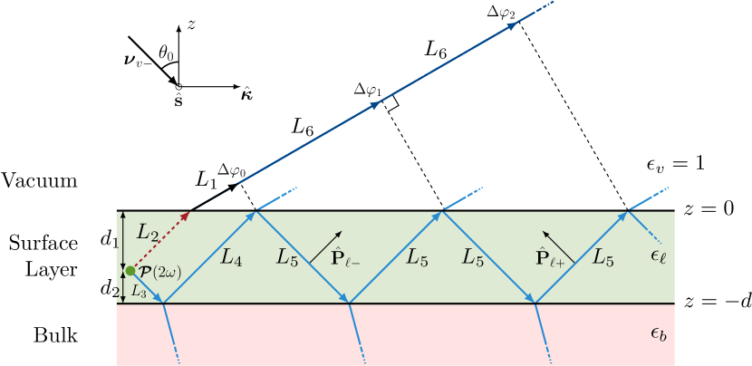
Figure 1: Sketch of the three layer model for SHG.

To begin our derivation of our model, we follow Ref. mizrahiJOSA88 and assume a polarization sheet located at $z_{\beta}$, of the form

$$\mathbf{P}(\mathbf{r},t)=\boldsymbol{\mathcal{P}}e^{i\boldsymbol{\kappa}\cdot\mathbf{R}}e^{-i\omega t}\delta(z-z_{\beta})+\mathrm{c.c.},$$ (3)

where $\mathbf{R}=(x,y)$, $\boldsymbol{\kappa}$ is the component of the wave vector $\boldsymbol{\nu}^{\phantom{a}}_{\beta}$ parallel to the surface, and $z_{\beta}$ is the position of the sheet within medium $\beta$, and $\boldsymbol{\mathcal{P}}$ is the position-independent polarization. Ref. sipeJOSAB87 demonstrates that the solution of the Maxwell equations for the radiated fields $E_{\beta,p\pm}$, and $E_{\beta,s}$ with $\mathbf{P}(\mathbf{r},t)$ as a source at points $z\neq 0$, can be written as

$$(E_{\beta,p\pm},E_{\beta,s})=(\frac{\gamma i\tilde{\omega}^{2}}{2\epsilon_{0}\tilde{w}_{\beta}}\,\hat{\mathbf{p}}_{\beta\pm}\cdot\boldsymbol{\mathcal{P}},\frac{\gamma i\tilde{\omega}^{2}}{2\epsilon_{0}\tilde{w}_{\beta}}\,\hat{\mathbf{s}}\cdot\boldsymbol{\mathcal{P}}),$$ (4)

where $\tilde{\omega}=\omega/c$; $\hat{\mathbf{s}}$ and $\hat{\mathbf{p}}_{\beta\pm}$ are the unit vectors for the $s$ and $p$ polarizations of the radiated field, respectively. The $\pm$ refers to upward ($+$) or downward ($-$) direction of propagation within medium $\beta$, as described in Fig. 1. Also, $\tilde{w}^{\phantom{a}}_{\beta}(\omega)=\tilde{\omega}w^{\phantom{a}}_{\beta}$, where

$$\hat{\mathbf{p}}^{\phantom{A}}_{\beta\pm}(\omega)=\frac{\kappa(\omega)\hat{\mathbf{z}}\mp\tilde{w}^{\phantom{A}}_{\beta}(\omega)\hat{\boldsymbol{\kappa}}}{\tilde{\omega}n^{\phantom{A}}_{\beta}(\omega)}=\frac{\sin\theta_{0}\hat{\mathbf{z}}\mp w^{\phantom{A}}_{\beta}(\omega)\hat{\boldsymbol{\kappa}}}{n^{\phantom{A}}_{\beta}(\omega)},$$ (5)

with

$$w^{\phantom{a}}_{\beta}(\omega)=\big{(}\epsilon^{\phantom{a}}_{\beta}(\omega)-\sin^{2}\theta_{0}\big{)}^{1/2},$$ (6)

$\theta_{0}$ is the angle of incidence of $\mathbf{E}_{v}(\omega)$, $\kappa(\omega)=|\boldsymbol{\kappa}|=\tilde{\omega}\sin\theta_{0}$, $n^{\phantom{A}}_{\beta}(\omega)=\sqrt{\epsilon^{\phantom{A}}_{\beta}(\omega)}$ is the index of refraction of medium $\beta$, and $z$ is the direction perpendicular to the surface that points towards the vacuum. If we consider the plane of incidence along the $\boldsymbol{\kappa}z$ plane, then

$$\hat{\boldsymbol{\kappa}}=\cos\phi\hat{\mathbf{x}}+\sin\phi\hat{\mathbf{y}},$$ (7)

and

$$\hat{\mathbf{s}}=-\sin\phi\hat{\mathbf{x}}+\cos\phi\hat{\mathbf{y}},$$ (8)

where $\phi$ is the azimuthal angle with respect to the $x$ axis.

The nonlinear polarization responsible for the SHG is immersed in the thin layer ($\beta=\ell$), and is given by

$$\mathcal{P}^{\mathrm{a}}_{\ell}(2\omega)=\epsilon_{0}\chi^{\mathrm{abc}}_{\mathrm{surface}}(-2\omega;\omega,\omega)E^{\mathrm{b}}(\omega)E^{\mathrm{c}}(\omega),$$ (9)

where $\boldsymbol{\chi}_{\mathrm{surface}}(-2\omega;\omega,\omega)$ is the dipolar surface nonlinear susceptibility tensor; the calculation of this quantity is given in detail in Refs. andersonthesis and andersonPRB15 . We will omit the $(-2\omega;\omega,\omega)$ notation from this point on. The Cartesian indices $\mathrm{a,b,c}$ are summed over if repeated; $\chi^{\mathrm{abc}}=\chi^{\mathrm{acb}}$ is the intrinsic permutation symmetry due to the fact that SHG is degenerate in $E^{\mathrm{b}}(\omega)$ and $E^{\mathrm{c}}(\omega)$. As in Ref. mizrahiJOSA88 , we consider the polarization sheet (Eq. (3)) to be oscillating at some frequency $\omega$ in order to properly express Eqs. (4)–(8). However, in the following we find it convenient to use $\omega$ exclusively to denote the fundamental frequency and $\boldsymbol{\kappa}$ to denote the component of the incident wave vector parallel to the surface. The generated nonlinear polarization is oscillating at $\Omega=2\omega$ and will be characterized by a wave vector parallel to the surface $\mathbf{K}=2\boldsymbol{\kappa}$. We can carry over Eqs. (3)–(8) simply by replacing the lowercase symbols ($\omega,\tilde{\omega},\boldsymbol{\kappa},n^{\phantom{A}}_{\beta},\tilde{w}^{\phantom{A}}_{\beta},w^{\phantom{A}}_{\beta},\hat{\mathbf{p}}^{\phantom{A}}_{\beta\pm},\hat{\mathbf{s}}$) with uppercase symbols ($\Omega,\tilde{\Omega},\mathbf{K},N^{\phantom{A}}_{\beta},\tilde{W}^{\phantom{A}}_{\beta},W^{\phantom{A}}_{\beta},\hat{\mathbf{P}}_{\beta\pm},\hat{\mathbf{S}}$), all evaluated at $2\omega$. Of course, we always have that $\hat{\mathbf{S}}=\hat{\mathbf{s}}$.

From Fig. 1, we observe the propagation of the SH field as it is refracted at the layer-vacuum interface ($\ell v$), and reflected multiple times from the layer-bulk ($\ell b$) and layer-vacuum ($\ell v$) interfaces. Thus, we can define

$$\mathbf{T}^{\ell v}=\hat{\mathbf{s}}T_{s}^{\ell v}\hat{\mathbf{s}}+\hat{\mathbf{P}}_{v+}T_{p}^{\ell v}\hat{\mathbf{P}}_{\ell+},$$ (10)

as the transmission tensor for the $\ell v$ interface,

$$\mathbf{R}^{\ell b}=\hat{\mathbf{s}}R_{s}^{\ell b}\hat{\mathbf{s}}+\hat{\mathbf{P}}_{\ell+}R_{p}^{\ell b}\hat{\mathbf{P}}_{\ell-},$$ (11)

as the reflection tensor for the $\ell b$ interface, and

$$\mathbf{R}^{\ell v}=\hat{\mathbf{s}}R_{s}^{\ell v}\hat{\mathbf{s}}+\hat{\mathbf{P}}_{\ell-}R_{p}^{\ell v}\hat{\mathbf{P}}_{\ell+},$$ (12)

as the reflection tensor for the $\ell v$ interface. The Fresnel factors in uppercase letters, $T^{ij}_{s,p}$ and $R^{ij}_{s,p}$, are evaluated at $2\omega$ from the following well known formulas jacksonbook ,

$$\begin{split}t_{s}^{ij}(\omega)&=\frac{2w_{i}(\omega)}{w_{i}(\omega)+w_{j}(\omega)},\\ t_{p}^{ij}(\omega)&=\frac{2w_{i}(\omega)\sqrt{\epsilon_{i}(\omega)\epsilon_{j}(\omega)}}{w_{i}(\omega)\epsilon_{j}(\omega)+w_{j}(\omega)\epsilon_{i}(\omega)},\\ r_{s}^{ij}(\omega)&=\frac{w_{i}(\omega)-w_{j}(\omega)}{w_{i}(\omega)+w_{j}(\omega)},\\ r_{p}^{ij}(\omega)&=\frac{w_{i}(\omega)\epsilon_{j}(\omega)-w_{j}\epsilon_{i}(\omega)}{w_{i}(\omega)\epsilon_{j}(\omega)+w_{j}(\omega)\epsilon_{i}(\omega)}.\end{split}$$

With these expressions we easily derive the following useful relations,

$$\begin{split}1+r^{\ell b}_{s}&=t^{\ell b}_{s},\\ 1+r^{\ell b}_{p}&=\frac{n_{b}}{n_{\ell}}t^{\ell b}_{p},\\ 1-r^{\ell b}_{p}&=\frac{n_{\ell}}{n_{b}}\frac{w_{b}}{w_{\ell}}t^{\ell b}_{p},\\ t^{\ell v}_{p}&=\frac{w_{\ell}}{w_{v}}t^{v\ell}_{p},\\ t^{\ell v}_{s}&=\frac{w_{\ell}}{w_{v}}t^{v\ell}_{s}.\end{split}$$ (13)

II Multiple Reflections

II.1 Multiple SHG Reflections

The SH field $\mathbf{E}(2\omega)$ radiated by the SH polarization $\boldsymbol{\mathcal{P}}_{\ell}(2\omega)$ will radiate directly into the vacuum and the bulk, where it will be reflected back at the layer-bulk interface into the thin layer. This beam will be transmitted and reflected multiple times, as shown in Fig. 1. As the two beams propagate, a phase difference will develop between them according to

$$\begin{split}\Delta\varphi_{m}&=\tilde{\Omega}\Big{(}(L_{3}+L_{4}+2mL_{5})N_{\ell}\\ &\qquad\qquad-\big{(}L_{2}N_{\ell}+(L_{1}+mL_{6})N_{v}\big{)}\Big{)}\\ &=\delta_{0}+m\delta,\quad m=0,1,2,\ldots,\end{split}$$

where

$$\delta_{0}=8\pi\left(\frac{d_{2}}{\lambda_{0}}\right)W_{\ell},$$ (14)

and

$$\delta=8\pi\left(\frac{d}{\lambda_{0}}\right)W_{\ell},$$ (15)

where $\lambda_{0}$ is the wavelength of the fundamental field in the vacuum, $W_{\ell}$ is described in Eq. (6), $d$ is the thickness of layer $\ell$, and $d_{2}$ is the distance between $\boldsymbol{\mathcal{P}}_{\ell}(2\omega)$ and the $\ell b$ interface (see Fig. 1). We see that $\delta_{0}$ is the phase difference of the first and second transmitted beams, and $m\delta$ that of the first and third ($m=1$), first and fourth ($m=2$), and so on. Note that the thickness $d$ of the layer $\ell$ enters through the phase $\delta$, and the position $d_{2}$ of the nonlinear polarization $\mathbf{P}(\mathbf{r},t)$ (Eq. (3)) enters through $\delta_{0}$. In particular, $d_{2}$ could be used as a variable to study the effects of multiple reflections on the SSHG yield $\mathcal{R}(2\omega)$.

To take into account the multiple reflections of the generated SH field in the layer $\ell$, we proceed as follows. We only include the algebra for the $p$-polarized SH field, though the $s$-polarized field could be worked out along the same steps. The $p$-polarized $\mathbf{E}_{\ell,p}(2\omega)$ field reflected multiple times is given by

$$\begin{split}\mathbf{E}_{\ell,p}(2\omega)&=E_{\ell,p+}(2\omega)\mathbf{T}^{\ell v}\cdot\hat{\mathbf{P}}_{\ell+}+E_{\ell,p-}(2\omega)\mathbf{T}^{\ell v}\cdot\mathbf{R}^{\ell b}\cdot\hat{\mathbf{P}}_{\ell-}e^{i\Delta\varphi_{0}}\\ &+E_{\ell,p-}(2\omega)\mathbf{T}^{\ell v}\cdot\mathbf{R}^{\ell b}\cdot\mathbf{R}^{\ell v}\cdot\mathbf{R}^{\ell b}\cdot\hat{\mathbf{P}}_{\ell-}e^{i\Delta\varphi_{1}}\\ &+E_{\ell,p-}(2\omega)\mathbf{T}^{\ell v}\cdot\mathbf{R}^{\ell b}\cdot\mathbf{R}^{\ell v}\cdot\mathbf{R}^{\ell b}\cdot\mathbf{R}^{\ell v}\cdot\mathbf{R}^{\ell b}\cdot\hat{\mathbf{P}}_{\ell-}e^{i\Delta\varphi_{2}}+\cdots\\ &=E_{\ell,p+}(2\omega)\mathbf{T}^{\ell v}\cdot\hat{\mathbf{P}}_{\ell+}+E_{\ell,p-}(2\omega)\mathbf{T}^{\ell v}\cdot\sum_{m=0}^{\infty}\big{(}\mathbf{R}^{\ell b}\cdot\mathbf{R}^{\ell v}e^{i\delta}\Big{)}^{m}\cdot\mathbf{R}^{\ell b}\cdot\hat{\mathbf{P}}_{\ell-}e^{i\delta_{0}}.\end{split}$$

From Eqs. (10)–(12) it is easy to show that

$$\begin{split}\mathbf{T}^{\ell v}\cdot\Big{(}\mathbf{R}^{\ell b}\cdot\mathbf{R}^{\ell v}\Big{)}^{n}\cdot\mathbf{R}^{\ell b}&=\hat{\mathbf{s}}T^{\ell v}_{s}\Big{(}R^{\ell b}_{s}R^{\ell v}_{s}\Big{)}^{n}R^{\ell b}_{s}\hat{\mathbf{s}}\\ &+\hat{\mathbf{P}}_{v+}T^{\ell v}_{p}\Big{(}R^{\ell b}_{p}R^{\ell v}_{p}\Big{)}^{n}R^{\ell b}_{p}\hat{\mathbf{P}}_{\ell-},\end{split}$$

then,

$$\begin{split}\mathbf{E}_{\ell,p}(2\omega)&=\hat{\mathbf{P}}_{\ell+}T^{\ell v}_{p}\Big{(}E_{\ell,p+}(2\omega)\\ &\hskip 56.9055pt+\frac{R^{\ell b}_{p}e^{i\delta_{0}}}{1+R^{v\ell}_{p}R^{\ell b}_{p}e^{i\delta}}E_{\ell,p-}(2\omega)\Big{)},\end{split}$$

where we used $R^{ij}_{s,p}=-R^{ji}_{s,p}$. Using Eq. (4) and (13), we can readily write

$$\mathbf{E}_{\ell,p}(2\omega)=\frac{\gamma i\tilde{\Omega}}{W_{\ell}}\mathbf{H}_{\ell}\cdot\boldsymbol{\mathcal{P}}_{\ell}(2\omega),$$ (16)

where

$$\begin{split}\mathbf{H}_{\ell}&=\frac{W_{\ell}}{W_{v}}\Bigg{[}\hat{\mathbf{s}}\,T_{s}^{v\ell}\left(1+R^{M}_{s}\right)\hat{\mathbf{s}}\\ &\hskip 42.67912pt+\hat{\mathbf{P}}_{v+}T_{p}^{v\ell}\left(\hat{\mathbf{P}}_{\ell+}+R^{M}_{p}\hat{\mathbf{P}}_{\ell-}\right)\Bigg{]},\end{split}$$ (17)

and

$$R^{M}_{\mathrm{i}}\equiv\frac{R^{\ell b}_{\mathrm{i}}e^{i\delta_{0}}}{1+R^{v\ell}_{\mathrm{i}}R^{\ell b}_{\mathrm{i}}e^{i\delta}},\quad\mathrm{i}=s,p,$$ (18)

is defined as the multiple ($M$) reflection coefficient. This coefficient depends on the thickness $d$ of layer $\ell$, and most importantly on the position $d_{2}$ of $\boldsymbol{\mathcal{P}}_{\ell}(2\omega)$ within this layer. The final results will depend on both $d$ and $d_{2}$. However, using Eq. (14) we can also define an average $\bar{R}^{M}_{\mathrm{i}}$ as

$$\begin{split}\bar{R}^{M}_{\mathrm{i}}&\equiv\frac{1}{d}\int_{0}^{d}\frac{R^{\ell b}_{\mathrm{i}}e^{i(8\pi W_{\ell}/\lambda_{0})x}}{1+R^{v\ell}_{\mathrm{i}}R^{\ell b}_{\mathrm{i}}e^{i\delta}}\,dx\\ \\ &=\frac{R^{\ell b}_{\mathrm{i}}e^{i\delta/2}}{1+R^{v\ell}_{\mathrm{i}}R^{\ell b}_{\mathrm{i}}e^{i\delta}}\,\mathrm{sinc}(\delta/2),\end{split}$$

that only depends on $d$ through the $\delta$ term from Eq. (15). It is very convenient to go ahead and define

$$R^{M\pm}_{\mathrm{i}}\equiv 1\pm R^{M}_{\mathrm{i}},\quad\mathrm{i}=s,p.$$ (19)

To connect with the work in Ref. mizrahiJOSA88 , where $\boldsymbol{\mathcal{P}}(2\omega)$ is located on top of the vacuum-surface interface and only the vacuum radiated beam and the first (and only) reflected beam need be considered, we take $\ell=v$ and $d_{2}=0$, then $T^{\ell v}=1$, $R^{v\ell}=0$ and $\delta_{0}=0$, with which $R^{M}_{\mathrm{i}}=R^{vb}_{\mathrm{i}}$. Thus, Eq. (17) coincides with Eq. (3.8) of Ref. mizrahiJOSA88 .

II.2 Multiple Reflections for the Linear Field

We must also consider the multiple reflections of the fundamental field $\mathbf{E}_{\ell}(\omega)$ inside the thin layer $\ell$. In Fig. 2 we present the situation where $\mathbf{E}_{v}(\omega)$ impinges from the vacuum side along the $\hat{\boldsymbol{\kappa}}z$-plane. $\theta_{0}$ and $\boldsymbol{\nu}_{v-}$ are the angle of incidence and wave vector, respectively. The arrows point along the direction of propagation. The $p$-polarization unit vectors $\hat{\mathbf{p}}_{\beta\pm}$, point along the downward $(-)$ or upward $(+)$ directions and are denoted with thick arrows, where $\beta=v$ or $\ell$. The $s$-polarization unit vector $\hat{\mathbf{s}}$ points out of the page.

As the first transmitted beam is reflected multiple times from the $\ell b$ and the $\ell v$ interfaces, it accumulates a phase difference of $n\varphi$ (with $n=1,2,3,\ldots$) with respect to the incident field. $\varphi$ is given by

$$\begin{split}\varphi&=\frac{\omega}{c}(2L_{1}n_{\ell}-L_{2}n_{v})=4\pi\left(\frac{d}{\lambda_{0}}\right)w_{\ell},\end{split}$$ (20)

where $n_{v}=1$. We need Eqs. (11) and (12) for $1\omega$, and also need

$$\mathbf{t}^{v\ell}=\hat{\mathbf{s}}t_{s}^{v\ell}\hat{\mathbf{s}}+\hat{\mathbf{p}}_{\ell-}t_{p}^{v\ell}\hat{\mathbf{p}}_{v-},$$

to write

$$\begin{split}\mathbf{E}_{\ell}(\omega)&=E_{0}\Big{[}\mathbf{t}^{v\ell}+\mathbf{r}^{\ell b}\cdot\mathbf{t}^{v\ell}e^{i\varphi}+\mathbf{r}^{\ell b}\cdot\mathbf{r}^{\ell v}\cdot\mathbf{r}^{\ell b}\cdot\mathbf{t}^{v\ell}e^{i2\varphi}+\mathbf{r}^{\ell b}\cdot\mathbf{r}^{\ell v}\cdot\mathbf{r}^{\ell b}\cdot\mathbf{r}^{\ell v}\cdot\mathbf{r}^{\ell b}\cdot\mathbf{t}^{v\ell}e^{i3\varphi}+\cdots\Big{]}\cdot\hat{\mathbf{e}}^{\mathrm{i}}\\ &=E_{0}\Big{[}1+\Big{(}1+\mathbf{r}^{\ell b}\cdot\mathbf{r}^{\ell v}e^{i\varphi}+(\mathbf{r}^{\ell b}\cdot\mathbf{r}^{\ell v})^{2}e^{i2\varphi}+\cdots\Big{)}\cdot\mathbf{r}^{\ell b}e^{i\varphi}\Big{]}\cdot\mathbf{t}^{v\ell}\cdot\hat{\mathbf{e}}^{\mathrm{i}}\\ &=E_{0}\Big{[}\hat{\mathbf{s}}t^{v\ell}_{s}(1+r^{M}_{s})\hat{\mathbf{s}}+t^{v\ell}_{p}\left(\hat{\mathbf{p}}_{\ell-}+\hat{\mathbf{p}}_{\ell+}r^{M}_{p}\right)\hat{\mathbf{p}}_{v-}\Big{]}\cdot\hat{\mathbf{e}}^{\mathrm{i}},\end{split}$$

where $E_{0}$ is the intensity of the fundamental field, and $\hat{\mathbf{e}}^{\mathrm{i}}$ is the unit vector of the incoming polarization ($\mathrm{i}=s,p$), with $\hat{\mathbf{e}}^{s}=\hat{\mathbf{s}}$ and $\hat{\mathbf{e}}^{p}=\hat{\mathbf{p}}_{v-}$. Also,

$$r^{M}_{\mathrm{i}}\equiv\frac{r^{\ell b}_{\mathrm{i}}e^{i\varphi}}{1+r^{v\ell}_{\mathrm{i}}r^{\ell b}_{\mathrm{i}}e^{i\varphi}},\quad\mathrm{i}=s,p.$$ (21)

$r^{M}_{\mathrm{i}}$ is defined as the multiple (M) reflection coefficient for the fundamental field. We define $\mathbf{E}^{\mathrm{i}}_{\ell}(\omega)\equiv E_{0}\mathbf{e}^{\omega,\mathrm{i}}_{\ell}$ ($\mathrm{i}=s,p$), where

$$\mathbf{e}^{\omega,\mathrm{i}}_{\ell}=\Big{[}\hat{\mathbf{s}}t^{v\ell}_{s}(1+r^{M}_{s})\hat{\mathbf{s}}+t^{v\ell}_{p}\left(\hat{\mathbf{p}}_{\ell-}+\hat{\mathbf{p}}_{\ell+}r^{M}_{p}\right)\hat{\mathbf{p}}_{v-}\Big{]}\cdot\hat{\mathbf{e}}^{\mathrm{i}},$$

and using Eqs. (5), (7), and (8) we obtain that

$$\mathbf{e}^{\omega,i}_{\ell}=\Bigg{[}t^{v\ell}_{s}r^{M+}_{s}\left(-\sin\phi\hat{\mathbf{x}}+\cos\phi\hat{\mathbf{y}}\right)\hat{\mathbf{s}}+\frac{t^{v\ell}_{p}}{n_{\ell}}\left(r^{M+}_{p}\sin\theta_{0}\hat{\mathbf{z}}+r^{M-}_{p}w_{\ell}\cos\phi\hat{\mathbf{x}}+r^{M-}_{p}w_{\ell}\sin\phi\hat{\mathbf{y}}\right)\hat{\mathbf{p}}_{v-}\Bigg{]}\cdot\hat{\mathbf{e}}^{\mathrm{i}},$$ (22)

where

$$r^{M\pm}_{\mathrm{i}}=1\pm r^{M}_{\mathrm{i}},\quad\mathrm{i}=s,p.$$

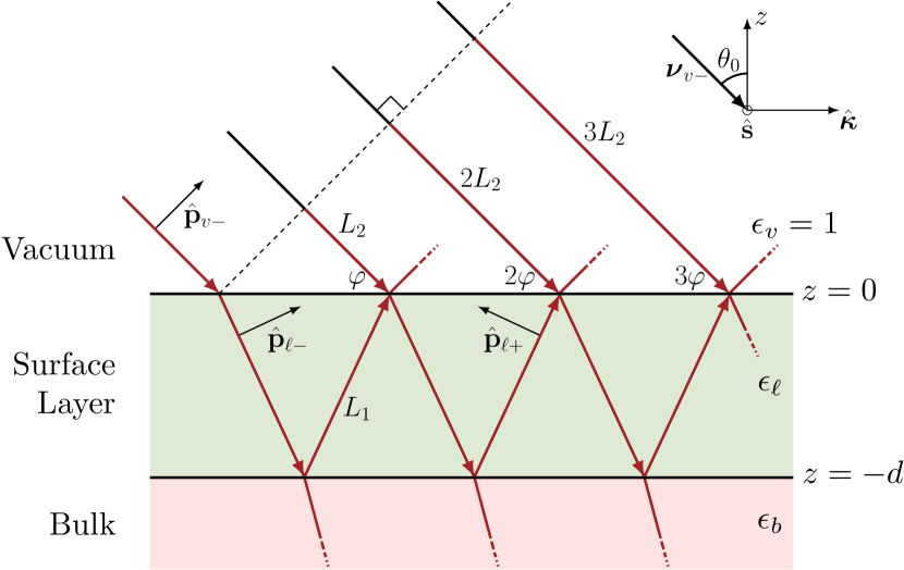
Figure 2: Sketch of the multiple reflected fundamental fields in the three layer model.

III General Polarization Considerations

III.1 $2\omega$ Terms for P and S Linear Polarization

The outgoing SHG radiation will almost always be measured in some configuration of $P$ and $S$ polarization. Using Eq. (13), we can write Eq. (16) as

$$\begin{split}E_{\ell}(2\omega)&=\frac{2\gamma i\omega}{cW_{\ell}}\hat{\mathbf{e}}^{\mathrm{F}}\cdot\mathbf{H}_{\ell}\cdot\boldsymbol{\mathcal{P}}_{\ell}(2\omega)\\ \\ &=\frac{2\gamma i\omega}{cW_{v}}\mathbf{e}^{\,2\omega,\mathrm{F}}_{\ell}\cdot\boldsymbol{\mathcal{P}}_{\ell}(2\omega),\end{split}$$ (23)

where

$$\begin{split}\mathbf{e}^{2\omega,\mathrm{F}}_{\ell}&=\hat{\mathbf{e}}^{\mathrm{F}}\cdot\Bigg{[}\hat{\mathbf{s}}T_{s}^{v\ell}R^{M+}_{s}\hat{\mathbf{s}}\\ &+\hat{\mathbf{P}}_{v+}\frac{T^{v\ell}_{p}}{N_{\ell}}\left(\sin\theta_{0}R^{M+}_{p}\hat{\mathbf{z}}-W_{\ell}R^{M-}_{p}\hat{\boldsymbol{\kappa}}\right)\Bigg{]},\end{split}$$ (24)

remembering that $R^{M\pm}_{p}$ was previously defined in Eq. (19). By substituting Eqs. (7) and (8) into Eq. (24), we obtain

$$\begin{split}\mathbf{e}^{2\omega,P}_{\ell}=\frac{T^{v\ell}_{p}}{N_{\ell}}\big{(}&-W_{\ell}R^{M-}_{p}\cos\phi\hat{\mathbf{x}}\\ &-W_{\ell}R^{M-}_{p}\sin\phi\hat{\mathbf{y}}\sin\theta_{0}R^{M+}_{p}\hat{\mathbf{z}}\big{)},\end{split}$$ (25)

for $P$ $(\hat{\mathbf{e}}^{\mathrm{F}}=\hat{\mathbf{P}}_{v+})$ outgoing polarization, and

$$\mathbf{e}^{2\omega,S}_{\ell}=T_{s}^{v\ell}R^{M+}_{s}\left(-\sin\phi\hat{\mathbf{x}}+\cos\phi\hat{\mathbf{y}}\right).$$ (26)

for $S$ $(\hat{\mathbf{e}}^{\mathrm{F}}=\hat{\mathbf{s}})$ outgoing polarization.

III.2 $1\omega$ Terms for for Elliptical Polarization

Up until this juncture, we have not assumed any given polarization for the incoming fields, other than that they must be in some combination of $p$ or $s$ polarization. But let us consider the most general polarization case, elliptical polarization, by establishing that byersPRB94

$$\hat{\mathbf{e}}^{\mathrm{i}}=\sin\alpha\,\hat{\mathbf{s}}+e^{i\tau}\cos\alpha\,\hat{\mathbf{p}}_{v-}.$$ (27)

Plugging this into Eq. (22) yields

$$\mathbf{e}^{\omega}_{\ell}=\Bigg{[}\sin\alpha\,t^{v\ell}_{s}r^{M+}_{s}\left(-\sin\phi\hat{\mathbf{x}}+\cos\phi\hat{\mathbf{y}}\right)+e^{i\tau}\cos\alpha\,\frac{t^{v\ell}_{p}}{n_{\ell}}\left(r^{M+}_{p}\sin\theta_{0}\hat{\mathbf{z}}+r^{M-}_{p}w_{\ell}\cos\phi\hat{\mathbf{x}}+r^{M-}_{p}w_{\ell}\sin\phi\hat{\mathbf{y}}\right)\Bigg{]}.$$ (28)

Thinking ahead, it will be very hand to have the expression for $\mathbf{e}^{\omega}_{\ell}\mathbf{e}^{\omega}_{\ell}$. Multiplying these terms out leads to the following expression,

$$\begin{split}\mathbf{e}^{\omega}_{\ell}\mathbf{e}^{\omega}_{\ell}&=\sin^{2}\alpha\,\left(t^{v\ell}_{s}r^{M+}_{s}\right)^{2}\big{(}\sin^{2}\phi\hat{\mathbf{x}}\hat{\mathbf{x}}+\cos^{2}\phi\hat{\mathbf{y}}\hat{\mathbf{y}}-2\sin\phi\cos\phi\hat{\mathbf{x}}\hat{\mathbf{y}}\big{)}\\ &+e^{2i\tau}\cos^{2}\alpha\,\left(\frac{t^{v\ell}_{p}}{n_{\ell}}\right)^{2}\bigg{(}\big{(}r^{M-}_{p}\big{)}^{2}w^{2}_{\ell}\cos^{2}\phi\hat{\mathbf{x}}\hat{\mathbf{x}}+\big{(}r^{M-}_{p}\big{)}^{2}w^{2}_{\ell}\sin^{2}\phi\hat{\mathbf{y}}\hat{\mathbf{y}}+\big{(}r^{M+}_{p}\big{)}^{2}\sin^{2}\theta_{0}\hat{\mathbf{z}}\hat{\mathbf{z}}\\ &\hskip 99.58464pt+2r^{M+}_{p}r^{M-}_{p}w_{\ell}\sin\theta_{0}\sin\phi\hat{\mathbf{y}}\hat{\mathbf{z}}+2r^{M+}_{p}r^{M-}_{p}w_{\ell}\sin\theta_{0}\cos\phi\hat{\mathbf{x}}\hat{\mathbf{z}}+2\big{(}r^{M-}_{p}\big{)}^{2}w^{2}_{\ell}\sin\phi\cos\phi\hat{\mathbf{x}}\hat{\mathbf{y}}\bigg{)}\\ &+2e^{i\tau}\sin\alpha\cos\alpha\,\frac{t^{v\ell}_{p}t^{v\ell}_{s}r^{M+}_{s}}{n_{\ell}}\Big{(}-r^{M-}_{p}w_{\ell}\sin\phi\cos\phi\hat{\mathbf{x}}\hat{\mathbf{x}}+r^{M-}_{p}w_{\ell}\sin\phi\cos\phi\hat{\mathbf{y}}\hat{\mathbf{y}}\\ &\hskip 128.0374pt+r^{M+}_{p}\sin\theta_{0}\cos\phi\hat{\mathbf{y}}\hat{\mathbf{z}}-r^{M+}_{p}\sin\theta_{0}\sin\phi\hat{\mathbf{x}}\hat{\mathbf{z}}+r^{M-}_{p}w_{\ell}\cos 2\phi\hat{\mathbf{x}}\hat{\mathbf{y}}\Big{)}.\end{split}$$ (29)

Given that the terms for $1\omega$ are now presented for the most general polarization case, we can easily recover the expressions for $p$ and $s$ linear polarization by plugging in the appropriate values for $\alpha$ and $\tau$ (featured in Table 1) into Eq. (29).

Table 1: Values for $\alpha$ and $\tau$ (see Eq. (27)) that yield common polarization cases.

Type		$\alpha$	$\tau$
Linear	$p$ ($\hat{\mathbf{p}}_{v-}$)	0	0
Linear	$s$ ($\hat{\mathbf{s}}$)	$\pi/2$	0
Linear	$p$ + $s$	$\pi/4$	0
Circular	Left	$\pi/4$	$-\pi/2$
Circular	Right	$\pi/4$	$+\pi/2$
Elliptical		Any	Any

IV The SSHG Yield

The magnitude of the radiated field is given by $E(2\omega)=\hat{\mathbf{e}}^{\mathrm{F}}\cdot\mathbf{E}_{\ell}(2\omega)$, where $\hat{\mathbf{e}}^{\mathrm{F}}$ is the unit vector of the final SH polarization with $\mathrm{F}=S,P$, where $\hat{\mathbf{e}}^{S}=\hat{\mathbf{s}}$ and $\hat{\mathbf{e}}^{P}=\hat{\mathbf{P}}_{v+}$. Replacing $\mathbf{E}_{\ell}(\omega)\to E_{0}\mathbf{e}^{\omega}_{\ell}$, in Eq. (9), we obtain that

$$\boldsymbol{\mathcal{P}}_{\ell}(2\omega)=\epsilon_{0}E^{2}_{0}\,\boldsymbol{\chi}_{\mathrm{surface}}:\mathbf{e}^{\omega}_{\ell}\mathbf{e}^{\omega}_{\ell},$$

where $\mathbf{e}^{\omega}_{\ell}$ is given by Eq. (28), and thus Eq. (23) reduces to ($W_{v}=\cos\theta_{0}$)

$$E_{\ell}(2\omega)=\frac{i\omega}{c\cos\theta_{0}}\mathbf{e}^{2\omega,\mathrm{F}}_{\ell}\cdot\boldsymbol{\chi}_{\mathrm{surface}}:\mathbf{e}^{\omega}_{\ell}\mathbf{e}^{\omega}_{\ell},$$

in MKS units. For ease of notation, we define

$$\Upsilon_{\mathrm{F}}(\alpha,\tau)\equiv\mathbf{e}^{2\omega,\mathrm{F}}_{\ell}\cdot\boldsymbol{\chi}_{\mathrm{surface}}:\mathbf{e}^{\omega}_{\ell}\mathbf{e}^{\omega}_{\ell},$$ (30)

where F stands for the outgoing polarization of the SH electric field given by $\hat{\mathbf{e}}^{\mathrm{F}}$ in Eq. (24), and the $\mathbf{e}^{\omega}_{\ell}\mathbf{e}^{\omega}_{\ell}$ term defines the incoming polarization of the fundamental electric field as established in Eq. (29).

From Eqs. (1) and (2) we obtain that,

$$\begin{split}|E(2\omega)|^{2}&=|E_{0}|^{4}\frac{\omega^{2}}{c^{2}W^{2}_{v}}\\ \frac{2\epsilon_{0}c|\sqrt{N_{v}}E(2\omega)|^{2}}{\left(2\epsilon_{0}c|\sqrt{n_{\ell}}E_{0}|^{2}\right)^{2}}&=\frac{1}{4\epsilon^{2}_{0}c^{2}}\frac{2\epsilon_{0}\omega^{2}}{c\cos^{2}\theta_{0}}\left|\frac{\sqrt{N_{v}}}{n^{2}_{\ell}}\Upsilon_{\mathrm{F}}(\alpha,\tau)\right|^{2}\\ \frac{I(2\omega)}{I^{2}(\omega)}&=\frac{\omega^{2}}{2\epsilon_{0}c^{3}\cos^{2}\theta_{0}}\left|\frac{\sqrt{N_{v}}}{n^{2}_{\ell}}\Upsilon_{\mathrm{F}}(\alpha,\tau)\right|^{2}\\ \mathcal{R}_{\mathrm{F}}(\alpha,\tau)&=\frac{\omega^{2}}{2\epsilon_{0}c^{3}\cos^{2}\theta_{0}}\left|\frac{1}{n_{\ell}}\Upsilon_{\mathrm{F}}(\alpha,\tau)\right|^{2}.\end{split}$$

Finally, we condense these results and establish the SSHG yield as

$$\mathcal{R}_{\mathrm{F}}(\alpha,\tau)=\frac{\omega^{2}}{2\epsilon_{0}c^{3}\cos^{2}\theta_{0}}\left|\frac{1}{n_{\ell}}\Upsilon_{\mathrm{F}}(\alpha,\tau)\right|^{2},$$ (31)

where $N_{v}=1$ and $W_{v}=\cos\theta_{0}$. $\boldsymbol{\chi}_{\mathrm{surface}}$ is given in m²/V in the MKS unit system, since it is a surface second order nonlinear susceptibility, and $\mathcal{R}$ is given in m²/W.

We now have everything we need to derive the explicit expressions for $\mathcal{R}$, by using Eqs. (31) and (30), for any polarization combination of incoming and outgoing fields. The crux of the matter now becomes how to calculate Eq. (30); fortunately, this term can be expressed in a highly elegant and flexible manner that greatly simplifies the required algebra. Remember, the four most common combinations of linear polarizations ($p$-in/$P$-out, $p$-in/$S$-out, $s$-in/$P$-out, and $s$-in/$S$-out) can be easily recovered from this treatment by using the values for $\alpha$ and $\tau$ listed in Table 1.

As mentioned before, it will be very convenient to switch all expressions over to their respective matrix representations. We will start by representing $\boldsymbol{\chi}$ in this manner. Disregarding all symmetry relations, we have

$$\boldsymbol{\chi}=\begin{pmatrix}\chi^{xxx}&\chi^{xyy}&\chi^{xzz}&|&\chi^{xyz}&\chi^{xxz}&\chi^{xxy}\\[3.0pt] \chi^{yxx}&\chi^{yyy}&\chi^{yzz}&|&\chi^{yyz}&\chi^{yxz}&\chi^{yxy}\\[3.0pt] \chi^{zxx}&\chi^{zyy}&\chi^{zzz}&|&\chi^{zyz}&\chi^{zxz}&\chi^{zxy}\end{pmatrix},$$ (32)

where all 18 independent components are accounted for, recalling that $\chi^{\mathrm{abc}}=\chi^{\mathrm{acb}}$ for SHG. Notice that the left hand block contains the components of $\chi^{\mathrm{abc}}$ where $b=c$, and the right hand block those where $b\neq c$. If, for example, you have a sample that is rotated with respect to the original crystal axes, the rotated $\chi^{\mathrm{abc}}$ components will be a combination of different components from the original system. In Appendix A, we derive the expressions for the rotated components; they can be substituted directly into the equations that follow in this section.

Concerning the $1\omega$ terms, we can readily express Eq. (29) as a combination of vectors,

$$\mathbf{e}^{\omega}_{\ell}\mathbf{e}^{\omega}_{\ell}=\mathbf{c}\,\mathbf{r}^{\omega}(\alpha,\tau),$$

where

$$\mathbf{c}=\big{(}\hat{\mathbf{x}}\hat{\mathbf{x}}\hskip 5.0pt\hat{\mathbf{y}}\hat{\mathbf{y}}\hskip 5.0pt\hat{\mathbf{z}}\hat{\mathbf{z}}\hskip 5.0pt\hat{\mathbf{y}}\hat{\mathbf{z}}\hskip 5.0pt\hat{\mathbf{x}}\hat{\mathbf{z}}\hskip 5.0pt\hat{\mathbf{x}}\hat{\mathbf{y}}\big{)},$$

and

$$\begin{split}\mathbf{r}^{\omega}&(\alpha,\tau)=\sin^{2}\alpha\,\left(t^{v\ell}_{s}r^{M+}_{s}\right)^{2}\begin{pmatrix}\sin^{2}\phi\\[8.0pt] \cos^{2}\phi\\[8.0pt] 0\\[8.0pt] 0\\[8.0pt] 0\\[8.0pt] -2\sin\phi\cos\phi\end{pmatrix}\\[10.0pt] &+e^{2i\tau}\cos^{2}\alpha\,\left(\frac{t^{v\ell}_{p}}{n_{\ell}}\right)^{2}\begin{pmatrix}\left(r^{M-}_{p}\right)^{2}w^{2}_{\ell}\cos^{2}\phi\\[8.0pt] \left(r^{M-}_{p}\right)^{2}w^{2}_{\ell}\sin^{2}\phi\\[8.0pt] \left(r^{M+}_{p}\right)^{2}\sin^{2}\theta_{0}\\[8.0pt] 2r^{M+}_{p}r^{M-}_{p}w_{\ell}\sin\theta_{0}\sin\phi\\[8.0pt] 2r^{M+}_{p}r^{M-}_{p}w_{\ell}\sin\theta_{0}\cos\phi\\[8.0pt] 2\left(r^{M-}_{p}\right)^{2}w^{2}_{\ell}\sin\phi\cos\phi\end{pmatrix}\\[10.0pt] &+2e^{i\tau}\sin\alpha\cos\alpha\,\frac{t^{v\ell}_{p}t^{v\ell}_{s}r^{M+}_{s}}{n_{\ell}}\begin{pmatrix}-r^{M-}_{p}w_{\ell}\sin\phi\cos\phi\\[8.0pt] r^{M-}_{p}w_{\ell}\sin\phi\cos\phi\\[8.0pt] 0\\[8.0pt] r^{M+}_{p}\sin\theta_{0}\cos\phi\\[8.0pt] -r^{M+}_{p}\sin\theta_{0}\sin\phi\\[8.0pt] r^{M-}_{p}w_{\ell}\cos 2\phi\end{pmatrix}.\end{split}$$ (33)

Likewise, we can obtain the $2\omega$ terms from Eqs. (25) and (26), as

$$\mathbf{e}^{2\omega,\mathrm{F}}_{\ell}=\mathbf{C}\,\mathbf{R}^{2\omega,\mathrm{F}},$$

where

$$\mathbf{C}=\big{(}\hat{\mathbf{x}}\hskip 5.0pt\hat{\mathbf{y}}\hskip 5.0pt\hat{\mathbf{z}}\big{)},$$

and

$$\mathbf{R}^{2\omega,\mathrm{F}}=\left\{\begin{array}[]{ l }T^{v\ell}_{p}N_{\ell}^{-1}\begin{pmatrix}-R^{M-}_{p}W_{\ell}\cos\phi\\[3.0pt] -R^{M-}_{p}W_{\ell}\sin\phi\\[3.0pt] +R^{M+}_{p}\sin\theta_{0}\end{pmatrix},\,\text{for F $=P$},\\ \\ \\ T_{s}^{v\ell}R^{M+}_{s}\begin{pmatrix}-\sin\phi\\ \cos\phi\\ 0\end{pmatrix},\,\text{for F $=S$}.\end{array}\right.$$ (34)

Finally, we can express $\Upsilon_{\mathrm{F}}(\alpha,\tau)$ (Eq. (30)) in complete matrix form as follows,

$$\Upsilon_{\mathrm{F}}(\alpha,\tau)=\mathbf{R}^{2\omega,\mathrm{F}}\circ\boldsymbol{\chi}\cdot\mathbf{r}^{\omega}(\alpha,\tau),$$

where we use Eqs. (32), (33), and (34), and the “$\circ$” symbol is the Hadamard (piecewise) matrix product. Thus, we select the polarization of the incoming fields via $\alpha$ and $\tau$ in Eq. (33), and the output polarization can be either $P$ or $S$ in Eq. (34). The surface symmetries will be taken into account via $\boldsymbol{\chi}$ in Eq. (32), or we can neglect them entirely by calculating every $\chi^{\mathrm{abc}}$ component. The avid reader will want to consult Refs. andersonPRB16b and andersonthesis for the complete derivations of the expressions for different combinations of linear polarization, for three common surface symmetries.

V Conclusions

In this manuscript, we have developed complete matrix expressions for the SSHG radiation using the three layer model to describe the radiating system. This new treatment now considers the most general polarization case for the incoming fields, elliptical polarization. It also includes all required components of $\chi^{\mathrm{abc}}$, regardless of symmetry considerations. Thus, these expressions can be applied to any surface, regardless of symmetry and for any choice of incoming polarization. This inherent flexibility of the model makes it an excellent choice for thin films and 2D materials. Details about the software implementation of the theory developed here can be found in Ref. andersonJOSS17 .

Appendix A Considering an arbitrary rotation on $\boldsymbol{\chi}(-2\omega;\omega,\omega)$

To take the components of $\boldsymbol{\chi}(-2\omega;\omega,\omega)$ from the crystallographic frame to the lab frame, we can simply apply a standard rotational matrix,

$$R=\begin{pmatrix}R_{Xx}&R_{Xy}&R_{Xz}\\ R_{Yx}&R_{Yy}&R_{Yz}\\ R_{Zx}&R_{Zy}&R_{Zz}\\ \end{pmatrix}=\begin{pmatrix}\sin\gamma&-\cos\gamma&0\\ \cos\gamma&\sin\gamma&0\\ 0&0&1\end{pmatrix},$$

such that

$$\chi^{IJK}=\sum_{ijk}R_{Ii}R_{Jj}R_{Kk}\chi^{ijk},$$

where $I$, $J$, and $K$ ($i$, $j$, $k$) cycle through $X$, $Y$, or $Z$ ($x$, $y$, $z$). Fig. 3 depicts this rotation over any arbitrary angle $\gamma$. Since we only consider a rotation in the $xy$-plane along $\gamma$, the $z$ and $Z$ axes are the same.

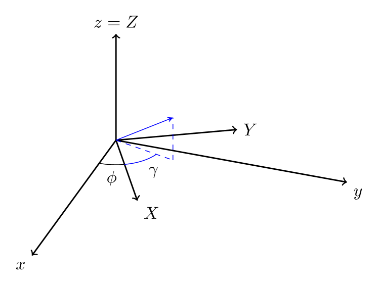
Figure 3: The translation from the non-rotated $xyz$ coordinates to the rotated $XYZ$ system.

Therefore, our $\chi^{IJK}$ components in terms of the original $ijk$ coordinate system are

$$\begin{split}\chi^{XXX}&=\sin^{3}\gamma\chi^{xxx}\\ &+\sin\gamma\cos^{2}\gamma\chi^{xyy}\\ &-2\sin^{2}\gamma\cos\gamma\chi^{xxy}\\ &-\sin^{2}\gamma\cos\gamma\chi^{yxx}\\ &-\cos^{3}\gamma\chi^{yyy}\\ &+2\sin\gamma\cos^{2}\gamma\chi^{yxy},\end{split}$$

$$\begin{split}\chi^{XYY}&=\sin\gamma\cos^{2}\gamma\chi^{xxx}\\ &+\sin^{3}\gamma\chi^{xyy}\\ &+2\sin^{2}\gamma\cos\gamma\chi^{xxy}\\ &-\cos^{3}\gamma\chi^{yxx}\\ &-\sin^{2}\gamma\cos\gamma\chi^{yyy}\\ &-2\sin\gamma\cos^{2}\gamma\chi^{yxy},\end{split}$$

$$\chi^{XZZ}=\sin\gamma\chi^{xzz}-\cos\gamma\chi^{yzz},$$

$$\begin{split}\chi^{XYZ}=\chi^{XZY}&=\sin^{2}\gamma\chi^{xyz}\\ &+\sin\gamma\cos\gamma\chi^{xxz}\\ &-\sin\gamma\cos\gamma\chi^{yyz}\\ &-\cos^{2}\gamma\chi^{yxz},\end{split}$$

$$\begin{split}\chi^{XXZ}=\chi^{XZX}&=-\sin\gamma\cos\gamma\chi^{xyz}\\ &+\sin^{2}\gamma\chi^{xxz}\\ &+\cos^{2}\gamma\chi^{yyz}\\ &-\sin\gamma\cos\gamma\chi^{yxz},\end{split}$$

$$\begin{split}\chi^{XXY}=\chi^{XYX}&=\sin^{2}\gamma\cos\gamma\chi^{xxx}\\ &-\sin^{2}\gamma\cos\gamma\chi^{xyy}\\ &+(\sin^{3}\gamma-\sin\gamma\cos^{2}\gamma)\chi^{xxy}\\ &-\sin\gamma\cos^{2}\gamma\chi^{yxx}\\ &+\sin\gamma\cos^{2}\gamma\chi^{yyy}\\ &+(\cos^{3}\gamma-\sin^{2}\gamma\cos\gamma)\chi^{yxy},\end{split}$$

for the $\chi^{XJK}$ components,

$$\begin{split}\chi^{YXX}&=\sin^{2}\gamma\cos\gamma\chi^{xxx}\\ &+\cos^{3}\gamma\chi^{xyy}\\ &-2\sin\gamma\cos^{2}\gamma\chi^{xxy}\\ &+\sin^{3}\gamma\chi^{yxx}\\ &+\sin\gamma\cos^{2}\gamma\chi^{yyy}\\ &-2\sin^{2}\gamma\cos\gamma\chi^{yxy},\end{split}$$

$$\begin{split}\chi^{YYY}&=\cos^{3}\gamma\chi^{xxx}\\ &+\sin^{2}\gamma\cos\gamma\chi^{xyy}\\ &+2\sin\gamma\cos^{2}\gamma\chi^{xxy}\\ &+\sin\gamma\cos^{2}\gamma\chi^{yxx}\\ &+\sin^{3}\gamma\chi^{yyy}\\ &+2\sin^{2}\gamma\cos\gamma\chi^{yxy},\end{split}$$

$$\chi^{YZZ}=\cos\gamma\chi^{xzz}+\sin\gamma\chi^{yzz},$$

$$\begin{split}\chi^{YYZ}=\chi^{YZY}&=\sin\gamma\cos\gamma\chi^{xyz}\\ &+\cos^{2}\gamma\chi^{xxz}\\ &+\sin^{2}\gamma\chi^{yyz}\\ &+\sin\gamma\cos\gamma\chi^{yxz},\end{split}$$

$$\begin{split}\chi^{YXZ}=\chi^{YZX}&=-\cos^{2}\gamma\chi^{xyz}\\ &+\sin\gamma\cos\gamma\chi^{xxz}\\ &-\sin\gamma\cos\gamma\chi^{yyz}\\ &+\sin^{2}\gamma\chi^{yxz},\end{split}$$

$$\begin{split}\chi^{YXY}=\chi^{YYX}&=\sin\gamma\cos^{2}\gamma\chi^{xxx}\\ &-\sin\gamma\cos^{2}\gamma\chi^{xyy}\\ &-(\cos^{3}\gamma-\sin^{2}\gamma\cos\gamma)\chi^{xxy}\\ &+\sin^{2}\gamma\cos\gamma\chi^{yxx}\\ &-\sin^{2}\gamma\cos\gamma\chi^{yyy}\\ &+(\sin^{3}\gamma-\sin\gamma\cos^{2}\gamma)\chi^{yxy},\end{split}$$

for the $\chi^{YJK}$ components, and lastly

$$\begin{split}\chi^{ZXX}&=\sin^{2}\gamma\chi^{zxx}\\ &+\cos^{2}\gamma\chi^{zyy}\\ &-2\sin\gamma\cos\gamma\chi^{zxy},\end{split}$$

$$\begin{split}\chi^{ZYY}&=\cos^{2}\gamma\chi^{zxx}\\ &+\sin^{2}\gamma\chi^{zyy}\\ &+2\sin\gamma\cos\gamma\chi^{zxy},\end{split}$$

$$\chi^{ZZZ}=\chi^{zzz},$$

$$\chi^{ZYZ}=\chi^{ZZY}=\sin\gamma\chi^{zyz}+\cos\gamma\chi^{zxz},$$

$$\chi^{ZXZ}=\chi^{ZZX}=-\cos\gamma\chi^{zyz}+\sin\gamma\chi^{zxz},$$

$$\begin{split}\chi^{ZXY}=\chi^{ZYX}&=\sin\gamma\cos\gamma\chi^{zxx}\\ &-\sin\gamma\cos\gamma\chi^{zyy}\\ &-\cos 2\gamma\chi^{zxy},\end{split}$$

for the $\chi^{ZJK}$ components. Fortunately, the intrinsic permutation symmetry of SHG is also present in the new coordinate system, such that $\chi^{IJK}=\chi^{IKJ}$; therefore, there are only 18 unique components in either system. Setting $\gamma=\pi/2$ signifies that there is no rotation, and thus $\chi^{IJK}=\chi^{ijk}$.

It should also be clear that the crystal symmetries do not follow into the rotated system. For instance, the $C_{3v}$ symmetry satisfies the following,

$$\begin{split}\chi^{xxx}&=-\chi^{xyy}=-\chi^{yxy},\\ \chi^{yxx}&=\chi^{yyy}=0.\end{split}$$

In the rotated system, the top relationship holds true such that $\chi^{XXX}=-\chi^{XYY}=-\chi^{YXY}$. However, we also obtain that

$$\chi^{YYY}=\cos 3\gamma\chi^{xxx},$$

which is not necessarily zero. Fortunately, we can simply apply the crystal symmetry to the non-rotated system before transforming to the rotated system. As an example case, we present $\chi^{XXX}$ for three values of $\gamma$ for a system with $C_{3v}$ symmetry in Fig. 4. The component in the original coordinates is recoverd when $\gamma=\pi/2$.

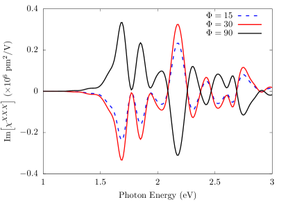
Figure 4: $\chi^{XXX}$ for three values of $\gamma$ calculated for a system with $C_{3v}$ symmetry.

References

[1]
S. M. Anderson and B. S. Mendoza.
Three-layer model for the surface second-harmonic generation yield
including multiple reflections.
Physical Review B, 94(11):115314, September 2016.
[2]
S. M. Anderson.
Theoretical Optical Second-Harmonic Calculations for Surfaces.
PhD thesis, Centro de Investigaciones en Óptica, A. C., Loma
del Bosque 115, Colonia Lomas del Campestre León, Guanajuato 37150,
Mexico, July 2016.
[3]
R.W. Boyd.
Nonlinear Optics.
Academic Press, New York, 2003.
[4]
Richard L. Sutherland.
Handbook of Nonlinear Optics.
CRC Press, April 2003.
[5]
V. Mizrahi and J. E. Sipe.
Phenomenological treatment of surface second-harmonic generation.
J. Opt. Soc. Am. B, 5(3):660–667, 1988.
[6]
J. E. Sipe.
New Green-function formalism for surface optics.
Journal of the Optical Society of America B, 4(4):481–489,
1987.
[7]
S. M. Anderson, N. Tancogne-Dejean, B. S. Mendoza, and V. Véniard.
Theory of surface second-harmonic generation for semiconductors
including effects of nonlocal operators.
Physical Review B, 91(7):075302, February 2015.
[8]
J. D. Jackson.
Classical Electrodynamics, 3rd Edition.
Wiley-VCH, 3rd edition edition, July 1998.
[9]
J. D. Byers, H. I. Yee, T. Petralli-Mallow, and J. M. Hicks.
Second-harmonic generation circular-dichroism spectroscopy from
chiral monolayers.
Phys. Rev. B, 49(20):14643, 1994.
[10]
S. M. Anderson and B. S. Mendoza.
SHGYield.
The Journal of Open Source Software, 2(14), June 2017.