Conductivity of graphene in the framework of Dirac model: Interplay between nonzero mass gap and chemical potential

Abstract

The complete theory of electrical conductivity of graphene at arbitrary temperature is developed with taken into account mass-gap parameter and chemical potential. Both the in-plane and out-of-plane conductivities of graphene are expressed via the components of the polarization tensor in (2+1)-dimensional space-time analytically continued to the real frequency axis. Simple analytic expressions for both the real and imaginary parts of the conductivity of graphene are obtained at zero and nonzero temperature. They demonstrate an interesting interplay depending on the values of mass gap and chemical potential. In the local limit, several results obtained earlier using various approximate and phenomenological approaches are reproduced, refined and generalized. The numerical computations of both the real and imaginary parts of the conductivity of graphene are performed to illustrate the obtained results. The analytic expressions for the conductivity of graphene obtained in this paper can serve as a guide in the comparison between different theoretical approaches and between experiment and theory.

I INTRODUCTION

The electrical conductivity of graphene, a two-dimensional hexagonal lattice of carbon atoms, possesses many qualities required for prospective applications in both fundamental physics and nanotechnology 1 ; 2 . At energies below a few electron volts the electronic properties of graphene are well described by the Dirac model 1 ; 2 ; 3 . In the context of this model graphene quasiparticles obey a linear dispersion relation, where the speed of light $c$ is replaced with the Fermi velocity $v_{F}\approx c/300$. The electrical properties of graphene are essentially connected with an existence of the so-called universal conductivity $\sigma_{0}$ expressed via the electron charge $e$ and Planck constant $\hbar$. For some time, a few distinct values for $\sigma_{0}$ have been obtained by different authors 4 ; 5 ; 6 ; 7 . Eventually a consensus was reached on the expression $\sigma_{0}=e^{2}/(4\hbar)$ 7 ; 8 ; 9 ; 10 ; 11 ; 12 ; 13 .

In general, the conductivity of graphene is nonlocal, i.e., depends on both the frequency and the magnitude of the wave vector, and also on the temperature. It was investigated by many authors using the phenomenological two-dimensional Drude model, the current-current correlation function in the random phase approximation, the Kubo response formalism, and the Boltzmann transport equation 1 ; 2 ; 3 ; 4 ; 5 ; 6 ; 7 ; 9 ; 10 ; 11 ; 12 ; 13 ; 14 ; 15 ; 16 ; 17 ; 18 ; 19 ; 20 ; 21 ; 22 ; 23 ; 24 ; 25 ; 26 ; 27 ; 27a ; 28 ; 29 ; 30 ; 31 ; 32 ; 33 ; 34 ; 35 . Furthermore, the electrical conductivity of graphene is sensitive to whether the mass of quasiparticles $m$ is exactly equal to zero or it is rather small but nonzero. For real graphene samples a nonzero mass gap $\Delta=2mc^{2}$ in the energy spectrum of quasiparticles arises under the influence of electron-electron interactions, substrates and impurities 3 ; 26 ; 36 ; 37 Some partial results for the conductivity of gapped graphene have been obtained using the two-band model 24 and the static polarization function 34 . In the local approximation at zero temperature the conductivity of gapped graphene was also examined in Refs. 12 ; 21 ; 22 .

Real graphene samples are always doped and can be characterized by some nonzero chemical potential $\mu$. The electrical conductivity of doped graphene was explored by using several approximate methods 12 ; 14 ; 24 ; 25 ; 29 ; 34 . The question arises of whether there are significant differences in impacts of the nonzero mass-gap parameter and chemical potential on the conductivity of graphene. On this subject it was noticed 12 that at zero temperature in the local approximation the response function for undoped but gapped graphene is similar to the case of doped but ungapped graphene if to identify the gap parameter, $\Delta$, with twice the Fermi energy, $2E_{F}$.

A comprehensive investigation of the conductivity of graphene can be performed using the exact expression for its polarization tensor at any temperature, mass gap and chemical potential. Although in some specific cases the polarization tensor in (2+1)-dimensional space-time has been calculated by many authors (see, e.g., Refs. 14 ; 26 ; 36 ; 38 ), the complete results needed for a fundamental understanding of the conductivity were obtained only recently. In Ref. 39 the exact polarization tensor of graphene with any mass-gap parameter has been found at zero temperature. The extension of this tensor to the case of nonzero temperature was made in Ref. 40 , but only at the pure imaginary Matsubara frequencies. The results of Refs. 39 ; 40 have been extensively used to calculate the Casimir force in graphene systems 41 ; 42 ; 43 ; 44 ; 45 ; 46 ; 47 ; 48 ; 49 ; 50 ; 51 , but they are not directly applicable in the studies of conductivity which is defined along the real frequency axis.

Another representation for the polarization tensor of gapped graphene, allowing an analytic continuation to the real frequency axis, was derived in Ref. 52 . It was applied in calculations of the Casimir force 53 ; 54 ; 55 ; 56 , on the one hand, and of the reflectivity properties of graphene and graphene-coated substrates 52 ; 57 ; 58 ; 59 , on the other hand. For the latter purposes, explicit expressions for the polarization tensor at real frequencies have been obtained for a gapless 52 ; 57 and gapped 58 graphene. This has opened up opportunities for a detailed study of the conductivity of graphene on the basis of first principles of quantum electrodynamics at nonzero temperature. The conductivity of pure (gapless) graphene was investigated in Ref. 60 using the continuation of the polarization tensor to real frequencies derived in Refs. 52 ; 57 . The case of gapped graphene was considered in Ref. 61 with the help of analytic continuation of the polarization tensor obtained for this case in Ref. 58 . In so doing, the previously known partial results for the conductivity of graphene have been reproduced and their generalizations to the case of any temperature with taken into account effects of nonlocality have been obtained.

In this paper, we develop the complete theory for the electrical conductivity of graphene in the framework of the Dirac model at arbitrary values of the mass gap, temperature and chemical potential. For this purpose, the results of Ref. 62 are used, where the polarization tensor of graphene of Ref. 52 was generalized to the case of graphene with nonzero chemical potential. We perform an analytic continuation of the polarization tensor of Ref. 62 to the real frequency axis and express both the longitudinal (in-plane) and transverse (perpendicular to the plane of graphene) conductivities in terms of its component. Then, the impact of chemical potential on the real part of conductivity at both zero and nonzero temperature is investigated. It is shown that at low frequencies satisfying a condition $\hbar\omega<\Delta$ the real part of conductivity of graphene is equal to zero at any values of temperature and chemical potential. For $\hbar\omega\geq\Delta$ the real part of conductivity is not equal to zero and there is an interesting interplay depending on the specific values of $\Delta$ and $\mu$. Thus, at zero temperature the real part of conductivity vanishes for $\hbar\omega<2\mu$ and is a simple function of $\sigma_{0}$, $\omega$, and $\Delta$ for $\hbar\omega>2\mu$. At nonzero temperature the real part of conductivity depends explicitly on $\sigma_{0}$, $\omega$, $T$, $\Delta$, and $\mu$. For the imaginary part of conductivity, simple analytic expressions are obtained at zero temperature, and the results of numerical computations at nonzero temperature are presented again demonstrating an important interplay between the values of $\Delta$ and $\mu$. In all cases we consider both the exact results and their local limits. The obtained analytic expressions are compared with those found earlier in the literature in the framework of various theoretical approaches.

The paper is organized as follows. In Sec. II we present an exact formalism expressing the conductivity of gapped graphene with nonzero chemical potential at any temperature via the components of the polarization tensor defined along the real frequency axis. Section III investigates the impact of chemical potential on the real part of conductivity. Here, the imaginary part of the polarization tensor is expanded in powers of a small parameter. Both cases of nonzero and zero temperature are considered. In Sec. IV the impact of chemical potential on the imaginary part of conductivity of graphene is examined. Here, the main contribution to the real part of the polarization tensor is found and the cases of nonzero and zero temperature are considered. In Sec. V the reader will find our conclusions and a discussion of the obtained results. The Appendix contains the proof of several asymptotic relations used in Sec. IV.

II Exact formalism for arbitrary temperature, mass-gap parameter and chemical potential

The polarization tensor allows complete description for the response of a physical system to external electromagnetic field. Although the tensor used below is found in the one-loop approximation, we call the formalism under consideration exact implying that in the framework of this approximation the role of nonzero temperature, mass gap and chemical potential is taken into account precisely. We denote the polarization tensor of graphene as $\Pi_{mn}(\omega,k,T,\Delta,\mu)$, where $m,\,n=0,\,1,\,2$, $k=|\mbox{\boldmath$k$}|$ is the magnitude of the wave vector component parallel to graphene, and $T$ is the temperature. The standard definition of $\Pi_{mn}$ in terms of the spinor propagator can be found in the textbooks 63 ; 64 and, in application to graphene, in Refs. 39 ; 40 ; 60 .

It is known 39 ; 40 that only the two components of the polarization tensor are the independent quantities. In the literature the most frequently used quantities are $\Pi_{00}$ and $\Pi_{\rm tr}\equiv\Pi_{n}^{\,n}$. Instead of the latter, however, for our purposes it is more convenient to employ the following quantity:

$$\Pi(\omega,k,T,\Delta,\mu)=k^{2}\Pi_{\rm tr}(\omega,k,T,\Delta,\mu)+\left(\frac{\omega^{2}}{c^{2}}-k^{2}\right)\Pi_{00}(\omega,k,T,\Delta,\mu).$$ (1)

A knowledge of the polarization tensor allows one to find the conductivity of graphene. The reason is that both the longitudinal, $\sigma_{\|}$, and transverse, $\sigma_{\bot}$, conductivities of graphene can be expressed via the respective correlation functions (see, e.g., Refs. 65 ; 66 ). The latter in turn are directly connected with the polarization tensor 50 . Eventually, the in-plane and out-of-plane conductivities of graphene are given by 50 ; 60 ; 61

$$\sigma_{\|}(\omega,k,T,\Delta,\mu)=-i\frac{\omega}{4\pi\hbar k^{2}}\Pi_{00}{(\omega,k,T,\Delta,\mu)},$$

$$\sigma_{\bot}(\omega,k,T,\Delta,\mu)=i\frac{c^{2}}{4\pi\hbar\omega k^{2}}\Pi{(\omega,k,T,\Delta,\mu)}.$$ (2)

To find the conductivities of graphene from Eq. (2), we continue the polarization tensor of graphene with nonzero $\Delta$ and $\mu$ found in Ref. 62 to the real frequency axis. Following Ref. 62 , it is convenient to present the quantities $\Pi_{00}$ and $\Pi$ as the sums of two contributions

$$\Pi_{00}(\omega,k,T,\Delta,\mu)=\Pi_{00}^{(0)}(\omega,k,\Delta)+\Pi_{00}^{(1)}(\omega,k,T,\Delta,\mu),$$

$$\Pi(\omega,k,T,\Delta,\mu)=\Pi^{(0)}(\omega,k,\Delta)+\Pi^{(1)}(\omega,k,T,\Delta,\mu).$$ (3)

Here, the terms $\Pi_{00}^{(0)}$ and $\Pi^{(0)}$ describe the gapped ($\Delta\neq 0$) but undoped ($\mu=0$) graphene at $T=0$. The explicit expressions for these terms were obtained in Ref. 39 (see also Refs. 52 ; 61 for an explicit analytic continuation to the real frequency axis). They can be written in the form

$$\Pi_{00}^{(0)}(\omega,k,\Delta)=-\frac{2\alpha k^{2}c}{\omega^{2}\eta^{2}}\,\tilde{\Phi}(\omega,k,\Delta),$$

$$\Pi^{(0)}(\omega,k,\Delta)=\frac{2\alpha k^{2}}{c}\,\tilde{\Phi}(\omega,k,\Delta),$$ (4)

where $\alpha=e^{2}/(\hbar c)$ is the fine structure constant and the quantity $\eta$ is defined as

$$\eta=\eta(\omega,k)=\sqrt{1-\frac{v_{F}^{2}k^{2}}{\omega^{2}}}.$$ (5)

The function $\tilde{\Phi}$ along the axis of real frequencies is given by 52 ; 61

$$\tilde{\Phi}(\omega,k,\Delta)=\left\{\begin{array}[]{ll}\Delta-\hbar\omega\eta\left[1+\left(\frac{\Delta}{\hbar\omega\eta}\right)^{2}\right]{\rm arctanh}\frac{\hbar\omega\eta}{\Delta},&\hbar\omega\eta<\Delta,\\[8.53581pt] \Delta-\hbar\omega\eta\left[1+\left(\frac{\Delta}{\hbar\omega\eta}\right)^{2}\right]\left({\rm arctanh}\frac{\Delta}{\hbar\omega\eta}+i\frac{\pi}{2}\right),&\hbar\omega\eta\geq\Delta.\end{array}\right.$$ (6)

Note that this $\tilde{\Phi}$ is different from the function $\Phi$ in Refs. 52 ; 61 by a factor, which is taken into account in Eq. (4). According to Eqs. (4) and (6), the quantities $\Pi_{00}^{(0)}$ and $\Pi^{(0)}$ are real if $\hbar\omega\eta<\Delta$ and have both the real and imaginary parts if $\hbar\omega\eta\geq\Delta$.

The terms $\Pi_{00}^{(1)}$ and $\Pi^{(1)}$ on the right-hand sides of Eq. (3) take into consideration the dependences on the temperature and on the chemical potential. Note that these terms should not be confused with the thermal corrections because they may remain not equal to zero in the limiting case $T\to 0$ (see Secs. III and IV). The resulting contributions, which may also depend on $\Delta$, describe a dependence of the zero-temperature polarization tensor on the chemical potential. They should vanish in the limiting case $\mu\to 0$.

The explicit expressions for $\Pi_{00}^{(1)}$ and $\Pi^{(1)}$, found in Ref. 62 , were analytically continued to the real frequency axis following Refs. 52 ; 58 . For the imaginary parts of $\Pi_{00}^{(1)}$ and $\Pi^{(1)}$, the results are

$${\rm Im}\Pi_{00}^{(1)}{(\omega,k,T,\Delta,\mu)}=\frac{4\alpha\hbar c^{2}}{v_{F}^{2}\omega\eta}\,\theta(\hbar\omega\eta-\Delta)$$

$$~{}~{}\times\int_{u^{(-)}}^{u^{(+)}}\!\!du\left(\frac{1}{e^{\beta u+\frac{\mu}{k_{B}T}}+1}+\frac{1}{e^{\beta u-\frac{\mu}{k_{B}T}}+1}\right)\frac{(2cu-\omega)^{2}-v_{F}^{2}k^{2}}{\sqrt{v_{F}^{2}k^{2}A(\omega,k)-(2cu-\omega)^{2}}},$$

$${\rm Im}\Pi^{(1)}{(\omega,k,T,\Delta,\mu)}=\frac{4\alpha\hbar\omega\eta}{v_{F}^{2}}\,\theta(\hbar\omega\eta-\Delta)$$ (7)

$$~{}~{}\times\int_{u^{(-)}}^{u^{(+)}}\!\!du\left(\frac{1}{e^{\beta u+\frac{\mu}{k_{B}T}}+1}+\frac{1}{e^{\beta u-\frac{\mu}{k_{B}T}}+1}\right)\frac{(2cu-\omega)^{2}+v_{F}^{2}k^{2}[1-A(\omega,k)]}{\sqrt{v_{F}^{2}k^{2}A(\omega,k)-(2cu-\omega)^{2}}}.$$

Here, $\beta=\hbar c/(k_{B}T)$, $\theta(x)$ is the step function equal to unity for $x\geq 0$ and zero for $x<0$, and the following notations are introduced

$$u^{(\pm)}=\frac{1}{2c}[\omega\pm v_{F}k\sqrt{A(\omega,k)}],$$

$$A(\omega,k)=1-\left(\frac{\Delta}{\hbar\omega\eta}\right)^{2}.$$ (8)

Note that not only $u^{(+)}>0$ but, due to the condition $ck<\omega$, it is valid that $u^{(-)}>0$ as well.

The real parts of $\Pi_{00}^{(1)}$ and $\Pi^{(1)}$ on the right-hand sides of Eq. (3) are defined differently in different frequency regions. For the sake of brevity, we introduce the notations

$$B_{1}(x)=\frac{x^{2}-v_{F}^{2}k^{2}}{\sqrt{x^{2}-v_{F}^{2}k^{2}A(\omega,k)}},$$ (9)

$$B_{2}(x)=\frac{x^{2}+v_{F}^{2}k^{2}[1-A(\omega,k)]}{\sqrt{x^{2}-v_{F}^{2}k^{2}A(\omega,k)}}.$$

Then, for the frequencies satisfying the condition $\hbar\omega\eta<\Delta$, one obtains

$${\rm Re}\Pi_{00}^{(1)}{(\omega,k,T,\Delta,\mu)}=\frac{8\alpha\hbar c^{2}}{v_{F}^{2}}\int_{\Delta/(2\hbar c)}^{\infty}\!\!\!du\sum_{\kappa=\pm 1}\frac{1}{e^{\beta u+\kappa\frac{\mu}{k_{B}T}}+1}$$

$$~{}~{}\times\left\{1-\frac{1}{2\omega\eta}\left[B_{1}(2cu+\omega)-B_{1}(2cu-\omega)\right]\right\},$$

$${\rm Re}\Pi^{(1)}(\omega,k,T,\Delta,\mu)=\frac{8\alpha\hbar\omega^{2}}{v_{F}^{2}}\int_{\Delta/(2\hbar c)}^{\infty}\!\!\!du\sum_{\kappa=\pm 1}\frac{1}{e^{\beta u+\kappa\frac{\mu}{k_{B}T}}+1}$$

$$~{}~{}\times\left\{1-\frac{\eta}{2\omega}\left[B_{2}(2cu+\omega)-B_{2}(2cu-\omega)\right]\right\}.$$ (10)

Here and below we use an abbreviated notation for the sum of exponent-containing fractions which is written out in full in Eq. (7).

Now we present the real parts of $\Pi_{00}^{(1)}$ and $\Pi^{(1)}$ in the frequency region $\hbar\omega\eta\geq\Delta$. Here, the convenient expression for ${\rm Re}\Pi_{00}^{(1)}$ is the following:

$${\rm Re}\Pi_{00}^{(1)}(\omega,k,T,\Delta,\mu)=\frac{8\alpha\hbar c^{2}}{v_{F}^{2}}(I_{1}+I_{2}+I_{3}),$$ (11)

where the integrals $I_{n}$ are given by

$$I_{1}=\int_{\Delta/(2\hbar c)}^{u^{(-)}}\!\!\!du\sum_{\kappa=\pm 1}\frac{1}{e^{\beta u+\kappa\frac{\mu}{k_{B}T}}+1}$$

$$~{}~{}\times\left\{1-\frac{1}{2\omega\eta}\left[B_{1}(2cu+\omega)+B_{1}(2cu-\omega)\right]\right\},$$

$$I_{2}=\int_{u^{(-)}}^{u^{(+)}}\!\!\!du\sum_{\kappa=\pm 1}\frac{1}{e^{\beta u+\kappa\frac{\mu}{k_{B}T}}+1}$$

$$~{}~{}\times\left[1-\frac{1}{2\omega\eta}B_{1}(2cu+\omega)\right],$$ (12)

$$I_{3}=\int_{u^{(+)}}^{\infty}\!\!\!du\sum_{\kappa=\pm 1}\frac{1}{e^{\beta u+\kappa\frac{\mu}{k_{B}T}}+1}$$

$$~{}~{}\times\left\{1-\frac{1}{2\omega\eta}\left[B_{1}(2cu+\omega)-B_{1}(2cu-\omega)\right]\right\}.$$

A similar expression for ${\rm Re}\Pi^{(1)}$ in the interval $\hbar\omega\eta\geq\Delta$ reads

$${\rm Re}\Pi^{(1)}(\omega,k,T,\Delta,\mu)=\frac{8\alpha\hbar\omega^{2}}{v_{F}^{2}}(J_{1}+J_{2}+J_{3}),$$ (13)

where

$$J_{1}=\int_{\Delta/(2\hbar c)}^{u^{(-)}}\!\!\!du\sum_{\kappa=\pm 1}\frac{1}{e^{\beta u+\kappa\frac{\mu}{k_{B}T}}+1}$$

$$~{}~{}\times\left\{1-\frac{\eta}{2\omega}\left[B_{2}(2cu+\omega)+B_{2}(2cu-\omega)\right]\right\},$$

$$J_{2}=\int_{u^{(-)}}^{u^{(+)}}\!\!\!du\sum_{\kappa=\pm 1}\frac{1}{e^{\beta u+\kappa\frac{\mu}{k_{B}T}}+1}$$

$$~{}~{}\times\left[1-\frac{\eta}{2\omega}B_{2}(2cu+\omega)\right],$$ (14)

$$J_{3}=\int_{u^{(+)}}^{\infty}\!\!\!du\sum_{\kappa=\pm 1}\frac{1}{e^{\beta u+\kappa\frac{\mu}{k_{B}T}}+1}$$

$$~{}~{}\times\left\{1-\frac{\eta}{2\omega}\left[B_{2}(2cu+\omega)-B_{2}(2cu-\omega)\right]\right\}.$$

Note that Eqs. (7), (10), (12), and (14), which take into account the chemical potential of gapped graphene, are also immediately obtainable from the respective equations of Ref. 61 , devoted to the conductivity of gapped but undoped graphene, by the substitution

$$\frac{1}{e^{\beta u}+1}\to\frac{1}{2}\sum_{\kappa=\pm 1}\frac{1}{e^{\beta u+\kappa\frac{\mu}{k_{B}T}}+1}.$$ (15)

This substitution is in fact the standard procedure for introducing the chemical potential in thermal quantum field theory 67 .

As a result, graphene conductivities are presented by Eq. (2), where the quantities $\Pi_{00}$ and $\Pi$ are given by Eqs. (3), (4), (7), (10), (11), and (13). These equations are used below to investigate an interplay between the mass gap and chemical potential and their combine impact on the conductivity properties.

III Impact of chemical potential on real part of conductivity

According to the results of Sec. II, the polarization tensor of graphene along the real frequency axis is a complex function, i.e., it has both the real and imaginary parts. From Eq. (2) for the real parts of conductivities one obtains

$${\rm Re}\sigma_{\|}(\omega,k,T,\Delta,\mu)=\frac{\omega}{4\pi\hbar k^{2}}{\rm Im}\Pi_{00}{(\omega,k,T,\Delta,\mu)},$$

$${\rm Re}\sigma_{\bot}(\omega,k,T,\Delta,\mu)=-\frac{c^{2}}{4\pi\hbar\omega k^{2}}{\rm Im}\Pi{(\omega,k,T,\Delta,\mu)}.$$ (16)

In agreement with Eq. (3)

$${\rm Im}\Pi_{00}(\omega,k,T,\Delta,\mu)={\rm Im}\Pi_{00}^{(0)}(\omega,k,\Delta)+{\rm Im}\Pi_{00}^{(1)}(\omega,k,T,\Delta,\mu),$$

$${\rm Im}\Pi(\omega,k,T,\Delta,\mu)={\rm Im}\Pi^{(0)}(\omega,k,\Delta)+{\rm Im}\Pi^{(1)}(\omega,k,T,\Delta,\mu).$$ (17)

Here, the first contributions on the right-hand sides are found from Eqs. (4) and (6)

$${\rm Im}\Pi_{00}^{(0)}(\omega,k,\Delta)=\frac{\pi\alpha\hbar ck^{2}}{\omega\eta}\theta(\hbar\omega\eta-\Delta)\left[1+\left(\frac{\Delta}{\hbar\omega\eta}\right)^{2}\right],$$ (18)

$${\rm Im}\Pi^{(0)}(\omega,k,\Delta)=-\frac{\pi\alpha\hbar\omega k^{2}\eta}{c}\theta(\hbar\omega\eta-\Delta)\left[1+\left(\frac{\Delta}{\hbar\omega\eta}\right)^{2}\right].$$

Using Eq. (5) we expand Eq. (18) in powers of a small parameter $v_{F}/c\sim 3\times 10^{-3}$ preserving only the terms up to the second order

$${\rm Im}\Pi_{00}^{(0)}(\omega,k,\Delta)=\frac{\pi\alpha\hbar ck^{2}}{\omega}\theta(\hbar\omega\eta-\Delta)\left[\frac{(\hbar\omega)^{2}+\Delta^{2}}{(\hbar\omega)^{2}}+\frac{v_{F}^{2}k^{2}}{2\omega^{2}}\frac{(\hbar\omega)^{2}+3\Delta^{2}}{(\hbar\omega)^{2}}\right],$$ (19)

$${\rm Im}\Pi^{(0)}(\omega,k,\Delta)=-\frac{\pi\alpha\hbar\omega k^{2}}{c}\theta(\hbar\omega\eta-\Delta)\left[\frac{(\hbar\omega)^{2}+\Delta^{2}}{(\hbar\omega)^{2}}-\frac{v_{F}^{2}k^{2}}{2\omega^{2}}\frac{(\hbar\omega)^{2}-\Delta^{2}}{(\hbar\omega)^{2}}\right].$$

Taking into account that

$$\frac{v_{F}^{2}k^{2}}{\omega^{2}}=\frac{v_{F}^{2}}{c^{2}}\frac{c^{2}k^{2}}{\omega^{2}}<\frac{v_{F}^{2}}{c^{2}},$$ (20)

the nonlocal contributions in Eq. (19) are much smaller, as compared to the local ones.

The second contributions to Eq. (17) are given by Eq. (7). As can be seen from Eqs. (7) and (18), the imaginary parts of $\Pi_{00}$ and $\Pi$ and, thus, the real parts of the conductivity of graphene (16) are not equal to zero only in the frequency region satisfying a condition $\hbar\omega\eta\geq\Delta$. Below we obtain the expansions of ${\rm Im}\Pi_{00}^{(1)}$ and ${\rm Im}\Pi^{(1)}$ in powers of $v_{F}^{2}/c^{2}$ similar to Eq. (19).

III.1 Imaginary parts of contributions to the polarization tensor depending on chemical potential

To obtain the desired expansions, we start from Eq. (7) and introduce the new integration variable

$$\tau=\frac{2cu-\omega}{v_{F}k\sqrt{A(\omega,k)}}.$$ (21)

Then Eq. (7) takes the form

$${\rm Im}\Pi_{00}^{(1)}{(\omega,k,T,\Delta,\mu)}=-\frac{2\alpha\hbar ck^{2}}{\omega\eta}\,\theta(\hbar\omega\eta-\Delta)\!\int_{-1}^{1}\!\!\!d\tau\sum_{\kappa=\pm 1}\frac{1}{e^{\frac{\hbar\omega+2\kappa\mu}{2k_{B}T}+\gamma\tau}+1}\frac{1-A(\omega,k)\tau^{2}}{\sqrt{1-\tau^{2}}},$$ (22)

$${\rm Im}\Pi^{(1)}{(\omega,k,T,\Delta,\mu)}=\frac{2\alpha\hbar\omega\eta k^{2}}{c}\,\theta(\hbar\omega\eta-\Delta)\!\int_{-1}^{1}\!\!\!d\tau\sum_{\kappa=\pm 1}\frac{1}{e^{\frac{\hbar\omega+2\kappa\mu}{2k_{B}T}+\gamma\tau}+1}\frac{1-A(\omega,k)(1-\tau^{2})}{\sqrt{1-\tau^{2}}}.$$

Here, the following notation is introduced:

$$\gamma=\gamma(\omega,k,\Delta)=\frac{v_{F}k}{\omega}\frac{\hbar\omega}{2k_{B}T}\sqrt{A(\omega,k)}.$$ (23)

Now we preserve only the terms up to the second order in $v_{F}/c$ so that

$$\eta=1-\frac{v_{F}^{2}k^{2}}{2\omega^{2}},\quad\frac{1}{\eta}=1+\frac{v_{F}^{2}k^{2}}{2\omega^{2}},$$ (24)

$$A(\omega,k)=A_{0}-\frac{v_{F}^{2}k^{2}\Delta^{2}}{\hbar^{2}\omega^{4}},\quad A_{0}\equiv 1-\left(\frac{\Delta}{\hbar\omega}\right)^{2}.$$

Expanding also the exponent-containing fractions up to the second order in the small parameter $\gamma\tau\sim v_{F}/c$, one can rewrite Eq. (22) in the form

$${\rm Im}\Pi_{00}^{(1)}{(\omega,k,T,\Delta,\mu)}=-\frac{2\alpha\hbar ck^{2}}{\omega}\,\theta(\hbar\omega\eta-\Delta)\sum_{\kappa=\pm 1}\left\{\frac{1}{e^{\frac{\hbar\omega+2\kappa\mu}{2k_{B}T}}+1}\int_{-1}^{1}\!\!\!d\tau\frac{1-A_{0}\tau^{2}}{\sqrt{1-\tau^{2}}}\right.$$

$$~{}~{}~{}+\frac{v_{F}^{2}k^{2}}{2\omega^{2}}\left[\frac{1}{e^{\frac{\hbar\omega+2\kappa\mu}{2k_{B}T}}+1}\int_{-1}^{1}\!\!\!d\tau\frac{1-A_{0}\tau^{2}}{\sqrt{1-\tau^{2}}}+2\left(\frac{\Delta}{\hbar\omega}\right)^{2}\frac{1}{e^{\frac{\hbar\omega+2\kappa\mu}{2k_{B}T}}+1}\int_{-1}^{1}\!\!\!d\tau\frac{\tau^{2}}{\sqrt{1-\tau^{2}}}\right.$$

$$~{}~{}~{}~{}+2A_{0}\left(\frac{\hbar\omega}{2k_{B}T}\right)^{2}{\rm csch}^{3}\frac{\hbar\omega+2\kappa\mu}{2k_{B}T}{\rm sinh}^{4}\frac{\hbar\omega+2\kappa\mu}{4k_{B}T}\left.\left.\int_{-1}^{1}\!\!\!d\tau\tau^{2}\frac{1-A_{0}\tau^{2}}{\sqrt{1-\tau^{2}}}\vphantom{\frac{1}{e^{\frac{\hbar\omega+2\kappa\mu}{2k_{B}T}}}}\right]\right\},$$ (25)

$${\rm Im}\Pi^{(1)}{(\omega,k,T,\Delta,\mu)}=\frac{2\alpha\hbar\omega k^{2}}{c}\,\theta(\hbar\omega\eta-\Delta)\sum_{\kappa=\pm 1}\left\{\frac{1}{e^{\frac{\hbar\omega+2\kappa\mu}{2k_{B}T}}+1}\int_{-1}^{1}\!\!\!d\tau\frac{1-A_{0}(1-\tau^{2})}{\sqrt{1-\tau^{2}}}\right.$$

$$~{}~{}+\frac{v_{F}^{2}k^{2}}{2\omega^{2}}\left[-\frac{1}{e^{\frac{\hbar\omega+2\kappa\mu}{2k_{B}T}}+1}\int_{-1}^{1}\!\!\!d\tau\frac{1-A_{0}(1-\tau^{2})}{\sqrt{1-\tau^{2}}}+2\left(\frac{\Delta}{\hbar\omega}\right)^{2}\frac{1}{e^{\frac{\hbar\omega+2\kappa\mu}{2k_{B}T}}+1}\int_{-1}^{1}\!\!d\tau\sqrt{1-\tau^{2}}\right.$$

$$~{}~{}~{}~{}\left.\left.+2A_{0}\left(\frac{\hbar\omega}{2k_{B}T}\right)^{2}{\rm csch}^{3}\frac{\hbar\omega+2\kappa\mu}{2k_{B}T}{\rm sinh}^{4}\frac{\hbar\omega+2\kappa\mu}{4k_{B}T}\int_{-1}^{1}\!\!d\tau\tau^{2}\frac{1-A_{0}(1-\tau^{2})}{\sqrt{1-\tau^{2}}}\vphantom{\frac{1}{e^{\frac{\hbar\omega+2\kappa\mu}{2k_{B}T}}}}\right]\right\}.$$

Note that we have omitted the linear in $\gamma\tau$ terms which lead to zero results after an integration with respect to $\tau$.

Calculating all integrals in Eq. (25), one arrives at

$${\rm Im}\Pi_{00}^{(1)}{(\omega,k,T,\Delta,\mu)}=-\frac{\pi\alpha\hbar ck^{2}}{\omega}\,\theta(\hbar\omega\eta-\Delta)\sum_{\kappa=\pm 1}\left\{\frac{(\hbar\omega)^{2}+\Delta^{2}}{(\hbar\omega)^{2}}\frac{1}{e^{\frac{\hbar\omega+2\kappa\mu}{2k_{B}T}}+1}\right.$$

$$~{}~{}~{}+\frac{v_{F}^{2}k^{2}}{2\omega^{2}}\frac{(\hbar\omega)^{2}+3\Delta^{2}}{(\hbar\omega)^{2}}\left[\frac{1}{e^{\frac{\hbar\omega+2\kappa\mu}{2k_{B}T}}+1}\right.+\left.\left.\frac{(\hbar\omega)^{2}-\Delta^{2}}{2(2k_{B}T)^{2}}{\rm csch}^{3}\frac{\hbar\omega+2\kappa\mu}{2k_{B}T}{\rm sinh}^{4}\frac{\hbar\omega+2\kappa\mu}{4k_{B}T}\right]\right\},$$

$${\rm Im}\Pi^{(1)}{(\omega,k,T,\Delta,\mu)}=\frac{\pi\alpha\hbar\omega k^{2}}{c}\,\theta(\hbar\omega\eta-\Delta)\sum_{\kappa=\pm 1}\left\{\frac{(\hbar\omega)^{2}+\Delta^{2}}{(\hbar\omega)^{2}}\frac{1}{e^{\frac{\hbar\omega+2\kappa\mu}{2k_{B}T}}+1}\right.$$ (26)

$$~{}~{}~{}-\frac{v_{F}^{2}k^{2}}{2\omega^{2}}\frac{(\hbar\omega)^{2}-\Delta^{2}}{(\hbar\omega)^{2}}\left[\frac{1}{e^{\frac{\hbar\omega+2\kappa\mu}{2k_{B}T}}+1}\right.-\left.\left.\frac{3(\hbar\omega)^{2}+\Delta^{2}}{2(2k_{B}T)^{2}}{\rm csch}^{3}\frac{\hbar\omega+2\kappa\mu}{2k_{B}T}{\rm sinh}^{4}\frac{\hbar\omega+2\kappa\mu}{4k_{B}T}\right]\right\}.$$

These are the desired contributions to the imaginary parts of the polarization tensor of graphene depending on temperature and on the chemical potential.

III.2 Real part of conductivity at any temperature

In accordance with Eq. (17), the total imaginary part of the polarization tensor in the two lowest perturbation orders is obtained by a summation of Eq. (19) and (26). In making this summation we take into account that

$$\frac{1}{2}-\frac{1}{e^{y}+1}=\frac{1}{2}\,{\rm tanh}\frac{y}{2}$$ (27)

and obtain

$${\rm Im}\Pi_{00}{(\omega,k,T,\Delta,\mu)}=\frac{\pi\alpha\hbar ck^{2}}{\omega}\,\theta(\hbar\omega\eta-\Delta)\sum_{\kappa=\pm 1}\left\{\frac{(\hbar\omega)^{2}+\Delta^{2}}{2(\hbar\omega)^{2}}{\rm tanh}\frac{\hbar\omega+2\kappa\mu}{4k_{B}T}\right.$$

$$~{}~{}~{}+\frac{v_{F}^{2}k^{2}}{4\omega^{2}}\frac{(\hbar\omega)^{2}+3\Delta^{2}}{(\hbar\omega)^{2}}\left[{\rm tanh}\frac{\hbar\omega+2\kappa\mu}{4k_{B}T}-\left.\frac{(\hbar\omega)^{2}-\Delta^{2}}{4(k_{B}T)^{2}}{\rm csch}^{3}\frac{\hbar\omega+2\kappa\mu}{2k_{B}T}{\rm sinh}^{4}\frac{\hbar\omega+2\kappa\mu}{4k_{B}T}\right]\right\},$$

$${\rm Im}\Pi{(\omega,k,T,\Delta,\mu)}=-\frac{\pi\alpha\hbar\omega k^{2}}{c}\,\theta(\hbar\omega\eta-\Delta)\sum_{\kappa=\pm 1}\left\{\frac{(\hbar\omega)^{2}+\Delta^{2}}{2(\hbar\omega)^{2}}{\rm tanh}\frac{\hbar\omega+2\kappa\mu}{4k_{B}T}\right.$$ (28)

$$~{}~{}~{}-\frac{v_{F}^{2}k^{2}}{4\omega^{2}}\frac{(\hbar\omega)^{2}-\Delta^{2}}{(\hbar\omega)^{2}}\left[{\rm tanh}\frac{\hbar\omega+2\kappa\mu}{4k_{B}T}-\left.\frac{3(\hbar\omega)^{2}+\Delta^{2}}{4(k_{B}T)^{2}}{\rm csch}^{3}\frac{\hbar\omega+2\kappa\mu}{2k_{B}T}{\rm sinh}^{4}\frac{\hbar\omega+2\kappa\mu}{4k_{B}T}\right]\right\}.$$

Substituting Eq. (28) in Eq. (16), one obtains the final result for the conductivities of graphene with arbitrary mass gap and chemical potential at any temperature

$${\rm Re}\sigma_{\|}(\omega,k,T,\Delta,\mu)=\sigma_{0}\theta(\hbar\omega\eta-\Delta)\sum_{\kappa=\pm 1}\left\{\frac{(\hbar\omega)^{2}+\Delta^{2}}{2(\hbar\omega)^{2}}{\rm tanh}\frac{\hbar\omega+2\kappa\mu}{4k_{B}T}\right.$$

$$~{}~{}~{}+\frac{v_{F}^{2}k^{2}}{4\omega^{2}}\frac{(\hbar\omega)^{2}+3\Delta^{2}}{(\hbar\omega)^{2}}\left[{\rm tanh}\frac{\hbar\omega+2\kappa\mu}{4k_{B}T}-\left.\frac{(\hbar\omega)^{2}-\Delta^{2}}{4(k_{B}T)^{2}}{\rm csch}^{3}\frac{\hbar\omega+2\kappa\mu}{2k_{B}T}{\rm sinh}^{4}\frac{\hbar\omega+2\kappa\mu}{4k_{B}T}\right]\right\},$$

$${\rm Re}\sigma_{\bot}(\omega,k,T,\Delta,\mu)=\sigma_{0}\theta(\hbar\omega\eta-\Delta)\sum_{\kappa=\pm 1}\left\{\frac{(\hbar\omega)^{2}+\Delta^{2}}{2(\hbar\omega)^{2}}{\rm tanh}\frac{\hbar\omega+2\kappa\mu}{4k_{B}T}\right.$$ (29)

$$~{}~{}~{}-\frac{v_{F}^{2}k^{2}}{4\omega^{2}}\frac{(\hbar\omega)^{2}-\Delta^{2}}{(\hbar\omega)^{2}}\left[{\rm tanh}\frac{\hbar\omega+2\kappa\mu}{4k_{B}T}-\left.\frac{3(\hbar\omega)^{2}+\Delta^{2}}{4(k_{B}T)^{2}}{\rm csch}^{3}\frac{\hbar\omega+2\kappa\mu}{2k_{B}T}{\rm sinh}^{4}\frac{\hbar\omega+2\kappa\mu}{4k_{B}T}\right]\right\}.$$

The conductivities (29) are nonlocal, but the corrections to local results are of order $v_{F}^{2}/c^{2}\sim 10^{-5}$. The main contributions to the conductivity of graphene are obtained in the local limit

$${\rm Re}\sigma_{\|}(\omega,0,T,\Delta,\mu)={\rm Re}\sigma_{\bot}(\omega,0,T,\Delta,\mu)=\sigma_{0}\theta(\hbar\omega\eta-\Delta)$$

$$~{}~{}~{}~{}\times\frac{(\hbar\omega)^{2}+\Delta^{2}}{2(\hbar\omega)^{2}}\left({\rm tanh}\frac{\hbar\omega+2\mu}{4k_{B}T}+{\rm tanh}\frac{\hbar\omega-2\mu}{4k_{B}T}\right).$$ (30)

At high frequencies satisfying the condition $\hbar\omega\gg 2\mu$ Eq. (30) leads to

$${\rm Re}\sigma_{\|(\bot)}(\omega,0,T,\Delta,\mu)=\sigma_{0}\theta(\hbar\omega\eta-\Delta)\frac{(\hbar\omega)^{2}+\Delta^{2}}{(\hbar\omega)^{2}}{\rm tanh}\frac{\hbar\omega}{4k_{B}T}$$

$$~{}~{}~{}~{}~{}~{}~{}\times\left[1+\left(\frac{\mu}{2k_{B}T}{\rm sech}\frac{\hbar\omega}{4k_{B}T}\right)^{2}\right].$$ (31)

Alternatively, at low frequencies $\Delta<\hbar\omega\ll 2\mu$ one has from Eq. (30)

$${\rm Re}\sigma_{\|(\bot)}(\omega,0,T,\Delta,\mu)=\sigma_{0}\theta(\hbar\omega\eta-\Delta)\frac{(\hbar\omega)^{2}+\Delta^{2}}{(\hbar\omega)^{2}}\frac{\hbar\omega}{4k_{B}T}{\rm sech}^{2}\frac{\mu}{2k_{B}T}.$$ (32)

Note that the same dependence of the conductivity of graphene on the frequency, temperature and chemical potential, as presented inside the round brackets in Eq. (30), was obtained in Ref. 11 within the approximate approach starting from the Kubo formula (see also Ref. 68 where this dependence was found for the case $\mu=0$). In Ref. 69 Eq. (30) is contained for the case of gapless graphene, $\Delta=0$, and interpreted as originating from the interband transitions.

The analytic result (30), although simple, suggests rich set of dependences of the real part of conductivity of graphene on the temperature and chemical potential for various relationships between $\mu$ and $\Delta$. Before making numerical computations, we briefly discuss the typical values of $\Delta$ and $\mu$. For a free-standing or deposited on a substrate graphene sheet an upper bound for the mass gap was estimated as $\Delta<0.2\,$eV 3 ; 39 . The value of the chemical potential at zero temperature can be expressed via the doping concentration $n$ as 70

$$\mu=\hbar v_{F}\sqrt{\pi n}.$$ (33)

For example, for the doping concentrations $n\approx 7.5\times 10^{11}$ and $2\times 10^{13}\,\mbox{cm}^{-2}$ one obtains $\mu=0.1$ and 0.5 eV, respectively. In the experiment on measuring the Casimir interaction between a Au-coated sphere and a graphene-coated SiO₂ layer on the top of a Si plate it was found 71 that $n\approx 1.2\times 10^{10}\,\mbox{cm}^{-2}$, which leads from Eq. (33) to the upper bound of $\mu=0.02\,$eV. This experiment was performed in high vacuum. In the measurement of the optical conductivity of graphene on top of a SiO₂ substrate 69 a representative value of $\mu=0.1\,$eV has been used. Note also that we do not consider the disorder effects in the form of, e.g., the charged puddles violating translational invariance, which may arise due to substrate and environment in addition to a relatively homogeneous doping.

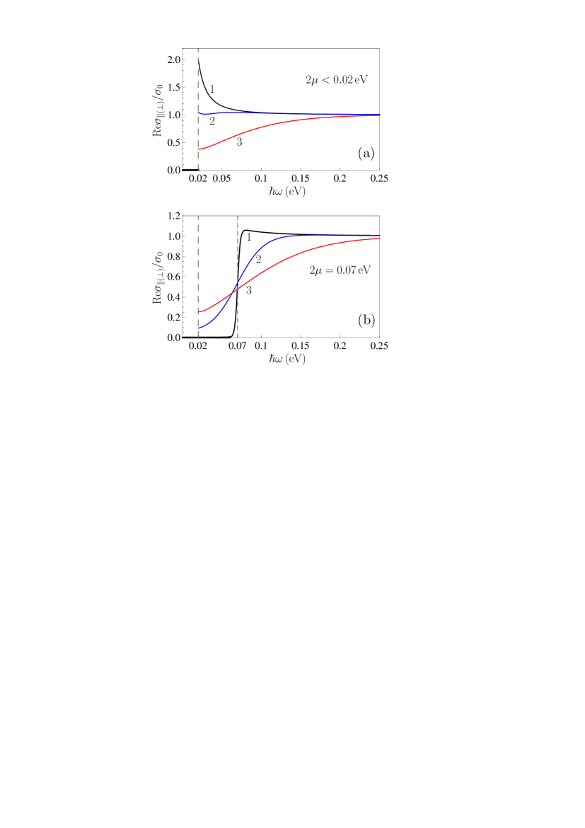
Figure 1: The real part of the conductivity of graphene with the mass gap $\Delta=0.02\,$eV normalized to the universal conductivity is shown as a function of frequency at $T=10\,$K, 100 K, and 300 K (lines 1, 2, and 3, respectively) for (a) any value of the chemical potential satisfying a condition $2\mu<0.02\,\mbox{eV}<\Delta$ and (b) $2\mu=0.07\,\mbox{eV}>\Delta$.

In Fig. 1 we plot the real part of the conductivity of graphene with the mass gap $\Delta=0.02\,$eV normalized to $\sigma_{0}$ as a function of frequency at $T=10\,$K, 100 K, and 300 K (lines 1, 2, and 3, respectively) for (a) any value of the chemical potential satisfying a condition $\mu<0.01\,$eV and (b) for $2\mu=0.07\,$eV. Note that the positions of lines in Fig. 1(a) do not depend on the specific value of $\mu$ in the indicated interval. In both Figs. 1(a) and 1(b) the real part of conductivity vanishes for $\hbar\omega<\Delta=0.02\,$eV. As is seen in Figs. 1(a) and 1(b), the character of ${\rm Re}\sigma_{\|(\bot)}$ as a function of frequency changes qualitatively depending on whether $2\mu<\Delta$ or $2\mu>\Delta$. Under these conditions the real part of conductivity of graphene behaves quite differently with decreasing temperature (see below for the case $T=0$). With increasing $\omega$ the real part of conductivity in all cases goes to the universal conductivity $\sigma_{0}$.

To illustrate the dependence of the real part of conductivity on the chemical potential, we introduce the quantity

$$\eta_{\mu}(\omega,T,\mu)=\frac{{\rm Re}\sigma_{\|(\bot)}(\omega,0,T,\Delta,\mu)}{{\rm Re}\sigma_{\|(\bot)}(\omega,0,T,\Delta,0)},$$ (34)

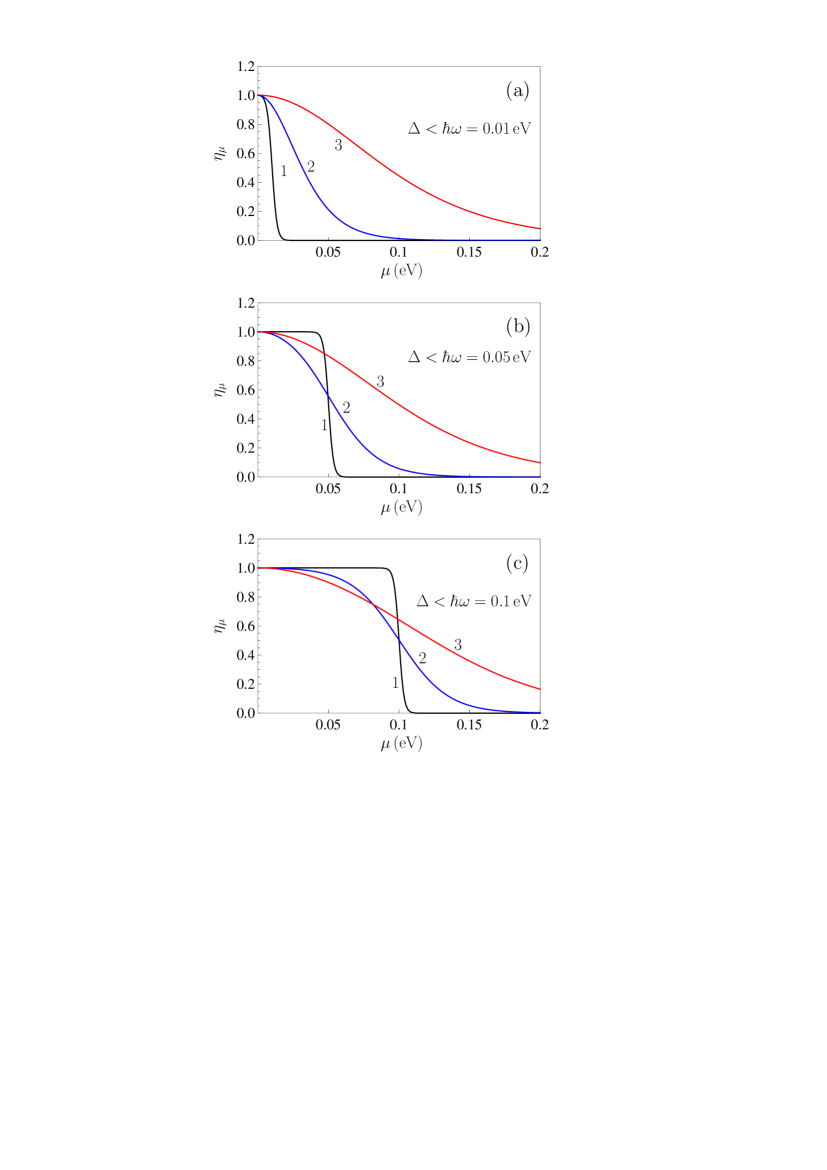
Figure 2: The real part of the conductivity of graphene normalized to its value at zero chemical potential is shown as a function of the chemical potential at $T=10\,$K, 100 K, and 300 K (lines 1, 2, and 3, respectively) for (a) $\hbar\omega=0.01\,$eV, (b) $\hbar\omega=0.05\,$eV, and (c) $\hbar\omega=0.1\,$eV.

which does not depend on the mass gap $\Delta$. In Fig. 2 we plot the quantity $\eta_{\mu}$ as a function of chemical potential at $T=10\,$K, 100 K, and 300 K (lines 1, 2, and 3, respectively) for the three values of frequency (a) $\hbar\omega=0.01\,$eV, (b) $\hbar\omega=0.05\,$eV, and (c) $\hbar\omega=0.1\,$eV. The respective possible values of the mass gap, for which the real part of conductivity does not vanish, satisfy the inequalities (a) $\Delta<0.01\,$eV, (b) $\Delta<0.05\,$eV, and (c) $\Delta<0.1\,$eV. As is seen in Fig. 2, the impact of chemical potential essentially depends on both the temperature and frequency taking into account also that the latter restricts the allowed values of the mass gap.

Now we consider the real part of the conductivity of graphene at zero temperature. For this purpose we take the limit $T\to 0$ in Eq. (29). It is easily seen that the last terms in both ${\rm Re}\sigma_{\|}$ and ${\rm Re}\sigma_{\bot}$, which contain ${\rm sinh}^{4}[(\hbar\omega+2\kappa\mu)/(4k_{B}T)]$, go to zero when $T$ goes to zero independently of the sign of $\kappa$. As to the function ${\rm tanh}[(\hbar\omega+2\kappa\mu)/(4k_{B}T)]$, it goes to unity when $T$ goes to zero if $\kappa=+1$, and also if $\kappa=-1$ and $\hbar\omega>2\mu$. If $\kappa=-1$ and $\hbar\omega<2\mu$ this function goes to minus unity with vanishing temperature. Taking all this into account, for $\hbar\omega>2\mu$ one obtains

$${\rm Re}\sigma_{\|}(\omega,k,0,\Delta,\mu)=\sigma_{0}\theta(\hbar\omega\eta-\Delta)$$

$$~{}~{}\times\left[\frac{(\hbar\omega)^{2}+\Delta^{2}}{(\hbar\omega)^{2}}+\frac{v_{F}^{2}k^{2}}{2\omega^{2}}\frac{(\hbar\omega)^{2}+3\Delta^{2}}{(\hbar\omega)^{2}}\right],$$

$${\rm Re}\sigma_{\bot}(\omega,k,0,\Delta,\mu)=\sigma_{0}\theta(\hbar\omega\eta-\Delta)$$ (35)

$$~{}~{}\times\left[\frac{(\hbar\omega)^{2}+\Delta^{2}}{(\hbar\omega)^{2}}-\frac{v_{F}^{2}k^{2}}{2\omega^{2}}\frac{(\hbar\omega)^{2}-\Delta^{2}}{(\hbar\omega)^{2}}\right].$$

These expressions are determined by only ${\rm Im}\Pi_{00}^{(0)}$ and ${\rm Im}\Pi^{(0)}$ defined in Eq. (19).

In the local limit for $\hbar\omega>2\mu$ the real part of the conductivity of graphene at zero temperature takes an especially simple form

$${\rm Re}\sigma_{\|}(\omega,0,0,\Delta,\mu)={\rm Re}\sigma_{\bot}(\omega,0,0,\Delta,\mu)=\sigma_{0}\theta(\hbar\omega\eta-\Delta)\frac{(\hbar\omega)^{2}+\Delta^{2}}{(\hbar\omega)^{2}}.$$ (36)

Alternatively, for $\hbar\omega<2\mu$ in the limiting case $T\to 0$ Eq. (29) leads to the vanishing real part of the conductivities of graphene

$${\rm Re}\sigma_{\|}(\omega,0,0,\Delta,\mu)={\rm Re}\sigma_{\bot}(\omega,0,0,\Delta,\mu)=0.$$ (37)

This result is determined by the canceled contributions from ${\rm Im}\Pi_{00}^{(0)}$, ${\rm Im}\Pi^{(0)}$, on the one hand, and ${\rm Im}\Pi_{00}^{(1)}$, ${\rm Im}\Pi^{(1)}$, on the other hand. For a gapped graphene with zero chemical potential Eq. (36) is presented in Ref. 12 (vanishing of the conductivity of gapped graphene at low frequencies was also noticed in Refs. 22 ; 24 ). In Ref. 61 Eqs. (35) and (36) were derived for the case of gapped but undoped ($\mu=0$) graphene using the formalism of the polarization tensor.

According to the above results (35)–(37), which are valid for both gapped and doped graphene, the real parts of graphene conductivities vanish in the frequency interval $[0,\max\{\Delta,2\mu\}/\hbar]$. In doing so, the magnitude of ${\rm Re}\sigma_{\|(\bot)}$ is always determined by the magnitude of the mass gap $\Delta$. In this sense there is no full symmetry between the cases of gapped, but undoped, and gapless, but doped, graphene mentioned in Sec. I if to identify $\Delta$ with $2E_{F}$ (recall that at $T=0$ the chemical potential $\mu$ is just the Fermi energy of the nonrelativistic electrons 70 ). Note that vanishing of the conductivity of graphene in the interval $[0,\max\{\Delta,2\mu\}/\hbar]$ was discussed in Ref. 22 .

The tendency toward vanishing of the real part of graphene conductivity in the interval mentioned above can be traced in Fig. 1(b), where with decreasing temperature (line 1 is plotted for $T=10\,$K) the right boundary of the range, where ${\rm Re}\sigma_{\|(\bot)}$ is zero approaches to $2\mu=0.07\,$eV. In Fig. 1(a), where $2\mu<\Delta$, this range is determined by $\Delta$ at all temperatures.

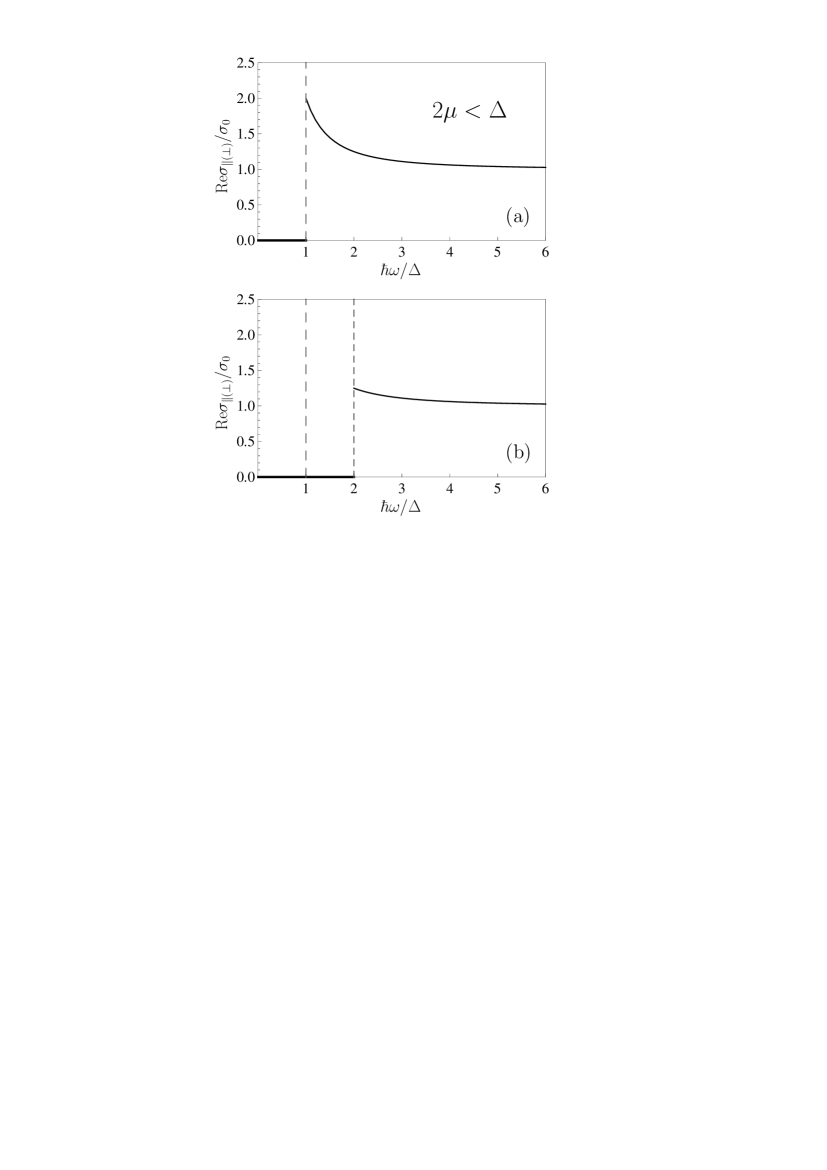
Figure 3: The real part of the conductivity of graphene normalized to the universal conductivity is shown as a function of $\hbar\omega/\Delta$ at zero temperature for (a) any value of the chemical potential satisfying a condition $2\mu<\Delta$ and (b) $\mu=\Delta$.

In Fig. 3 we illustrate the dependence ${\rm Re}\sigma_{\|(\bot)}$, normalized to the universal conductivity $\sigma_{0}$, on the dimensionless parameter $\hbar\omega/\Delta$. Figure 3(a) is plotted for the case $2\mu<\Delta$. Here, the frequency region where ${\rm Re}\sigma_{\|(\bot)}=0$ is $[0,\Delta/\hbar)$, i.e., is determined by the mass-gap parameter. In Fig. 3(b) the case $\mu=\Delta$ is considered. Now the region where ${\rm Re}\sigma_{\|(\bot)}=0$ is $[0,2\mu/\hbar)$, i.e., is determined by the value of chemical potential. In both Figs. 3(a) and 3(b), however, the magnitudes of ${\rm Re}\sigma_{\|(\bot)}$ are determined solely by the value of $\Delta$. In the limiting case of high frequencies ($\omega\to\infty$) the real part of the conductivity of graphene goes to the universal conductivity $\sigma_{0}$, as it should be on the basis of all previous knowledge.

IV Impact of chemical potential on imaginary part of conductivity

According to Eq. (2), the imaginary part of conductivity of graphene is expressed via the real part of polarization tensor

$${\rm Im}\sigma_{\|}(\omega,k,T,\Delta,\mu)=-\frac{\omega}{4\pi\hbar k^{2}}{\rm Re}\Pi_{00}{(\omega,k,T,\Delta,\mu)},$$

$${\rm Im}\sigma_{\bot}(\omega,k,T,\Delta,\mu)=\frac{c^{2}}{4\pi\hbar\omega k^{2}}{\rm Re}\Pi{(\omega,k,T,\Delta,\mu)}.$$ (38)

In accordance to Eq. (3)

$${\rm Re}\Pi_{00}(\omega,k,T,\Delta,\mu)={\rm Re}\Pi_{00}^{(0)}(\omega,k,\Delta)+{\rm Re}\Pi_{00}^{(1)}(\omega,k,T,\Delta,\mu),$$

$${\rm Re}\Pi(\omega,k,T,\Delta,\mu)={\rm Re}\Pi^{(0)}(\omega,k,\Delta)+{\rm Re}\Pi^{(1)}(\omega,k,T,\Delta,\mu).$$ (39)

The first contributions on the right-hand side of Eq. (39) are contained in Eqs. (4) and (6). They can be identically rewritten in a uniform way for both $\hbar\omega\eta<\Delta$ and $\hbar\omega\eta\geq\Delta$

$${\rm Re}\Pi_{00}^{(0)}(\omega,k,\Delta)=-\frac{2\alpha k^{2}c}{\omega^{2}\eta^{2}}\left\{\Delta-\frac{1}{2}\hbar\omega\eta\left[1+\left(\frac{\Delta}{\hbar\omega\eta}\right)^{2}\right]\ln\left|\frac{\hbar\omega\eta+\Delta}{\hbar\omega\eta-\Delta}\right|\right\},$$

$${\rm Re}\Pi^{(0)}(\omega,k,\Delta)=\frac{2\alpha k^{2}}{c}\left\{\Delta-\frac{1}{2}\hbar\omega\eta\left[1+\left(\frac{\Delta}{\hbar\omega\eta}\right)^{2}\right]\ln\left|\frac{\hbar\omega\eta+\Delta}{\hbar\omega\eta-\Delta}\right|\right\}.$$ (40)

Thus, the real parts of $\Pi_{00}^{(0)}$ and $\Pi^{(0)}$ are not equal to zero at all frequencies.

Now we take into account that due to Eq. (20) the nonlocal corrections to the conductivity of graphene are very small as compared to the main, local, contribution. Because of this, here we make all calculations in the lowest order of the small parameter $v_{F}^{2}k^{2}/\omega^{2}$. Thus, expanding Eq. (40) to the lowest order in this parameter, one obtains

$${\rm Re}\Pi_{00}^{(0)}(\omega,k,\Delta)=-\frac{2\alpha\hbar ck^{2}}{\omega}\left[\frac{\Delta}{\hbar\omega}-\frac{(\hbar\omega)^{2}+\Delta^{2}}{2(\hbar\omega)^{2}}\ln\left|\frac{\hbar\omega+\Delta}{\hbar\omega-\Delta}\right|\right],$$

$${\rm Re}\Pi^{(0)}(\omega,k,\Delta)=\frac{2\alpha\hbar\omega k^{2}}{c}\left[\frac{\Delta}{\hbar\omega}-\frac{(\hbar\omega)^{2}+\Delta^{2}}{2(\hbar\omega)^{2}}\ln\left|\frac{\hbar\omega+\Delta}{\hbar\omega-\Delta}\right|\right].$$ (41)

The second contributions on the right-hand side of Eq. (39) are given by Eqs. (10)–(14). They are also not equal to zero at all frequencies. We start from obtaining the main terms in the expansion of ${\rm Re}\Pi_{00}^{(1)}$ and ${\rm Re}\Pi^{(1)}$ in the powers of $v_{F}^{2}k^{2}/\omega^{2}$.

IV.1 Real parts of contributions to the polarization tensor depending on chemical potential

We consider first the frequency region $\hbar\omega\eta<\Delta$ which reduces to $\hbar\omega<\Delta$ in the lowest order of our small parameter. In this region ${\rm Re}\Pi_{00}^{(1)}$ and ${\rm Re}\Pi^{(1)}$ are given by Eq. (10). In the lowest order of the parameter $v_{F}^{2}k^{2}/\omega^{2}$ one has

$$1-\frac{1}{2\omega\eta}\left[B_{1}(2cu+\omega)-B_{1}(2cu-\omega)\right]$$

$$~{}~{}=-\frac{v_{F}^{2}k^{2}}{2\omega^{2}}\left[1+\frac{(\hbar\omega)^{2}+\Delta^{2}}{2(\hbar\omega)^{2}}\left(\frac{\omega}{2cu-\omega}-\frac{\omega}{2cu+\omega}\right)\right],$$

$$1-\frac{\eta}{2\omega}\left[B_{2}(2cu+\omega)-B_{2}(2cu-\omega)\right]$$ (42)

$$~{}~{}=\frac{v_{F}^{2}k^{2}}{2\omega^{2}}\left[1+\frac{(\hbar\omega)^{2}+\Delta^{2}}{2(\hbar\omega)^{2}}\left(\frac{\omega}{2cu-\omega}-\frac{\omega}{2cu+\omega}\right)\right],$$

Substituting Eq. (42) in Eq. (10) and introducing the new integration variable $t=2vu/\omega$, we arrive at

$${\rm Re}\Pi_{00}^{(1)}{(\omega,k,T,\Delta,\mu)}=-\frac{2\alpha\hbar ck^{2}}{\omega}\int_{\Delta/(\hbar\omega)}^{\infty}\!\!dt\sum_{\kappa=\pm 1}\frac{1}{e^{\frac{\hbar\omega t+2\kappa\mu}{2k_{B}T}}+1}$$

$$~{}~{}~{}~{}\times\left[1+\frac{(\hbar\omega)^{2}+\Delta^{2}}{(\hbar\omega)^{2}}\,\frac{1}{t^{2}-1}\right],$$

$${\rm Re}\Pi^{(1)}{(\omega,k,T,\Delta,\mu)}=\frac{2\alpha\hbar\omega k^{2}}{c}\int_{\Delta/(\hbar\omega)}^{\infty}\!\!dt\sum_{\kappa=\pm 1}\frac{1}{e^{\frac{\hbar\omega t+2\kappa\mu}{2k_{B}T}}+1}$$

$$~{}~{}~{}~{}\times\left[1+\frac{(\hbar\omega)^{2}+\Delta^{2}}{(\hbar\omega)^{2}}\,\frac{1}{t^{2}-1}\right].$$ (43)

Note that in the frequency region under consideration $\Delta/(\hbar\omega)>1$.

We are coming now to the case $\hbar\omega\eta\geq\Delta$ which reduces to $\hbar\omega\geq\Delta$ in the lowest perturbation order. Taking into account that in the lowest order the quantities ${\rm Re}\Pi_{00}^{(1)}$ and ${\rm Re}\Pi^{(1)}$ differ by only a factor in front of the integral [see Eq. (43)] we can restrict ourselves by considering ${\rm Re}\Pi_{00}^{(1)}$ defined in Eqs. (11) and (12). Then, the sum of the integrals defined in Eq. (12) is given by

$$I_{1}+I_{2}+I_{3}=-\frac{v_{F}^{2}k^{2}}{2\omega^{2}}\int_{\Delta/(2\hbar c)}^{\infty}\!\!du\sum_{\kappa=\pm 1}\frac{1}{e^{\beta u+\frac{\kappa\mu}{k_{B}T}}+1}$$

$$~{}~{}~{}~{}\times\left[1+\frac{(\hbar\omega)^{2}+\Delta^{2}}{2(\hbar\omega)^{2}}\,\left(\frac{\omega}{2cu-\omega}-\frac{\omega}{2cu+\omega}\right)\right]$$ (44)

$$~{}-\frac{1}{2}\int_{u^{(-)}}^{u^{(+)}}\!\!du\sum_{\kappa=\pm 1}\frac{1}{e^{\beta u+\frac{\kappa\mu}{k_{B}T}}+1}\left\{\frac{2cu-\omega}{\omega}+\frac{v_{F}^{2}k^{2}}{2\omega^{2}}\left[\frac{2cu-\omega}{\omega}-\frac{(2-A_{0})\omega}{2cu-\omega}\right]\right\}.$$

It can be easily seen that the second integral on the right-hand side of Eq. (44) is of the order of $v_{F}^{3}k^{3}/\omega^{3}$, i.e., should be omitted in our calculation. Then, substituting Eq. (44) in Eq. (11) and introducing the integration variable $t=2cu/\omega$, one obtains the real part of the $\mu$-dependent contribution to the polarization tensor

$${\rm Re}\Pi_{00}^{(1)}{(\omega,k,T,\Delta,\mu)}=-\frac{2\alpha\hbar ck^{2}}{\omega}\int_{\Delta/(\hbar\omega)}^{\infty}\!\!dt\sum_{\kappa=\pm 1}\frac{1}{e^{\frac{\hbar\omega t+2\kappa\mu}{2k_{B}T}}+1}$$

$$~{}~{}~{}~{}\times\left[1+\frac{(\hbar\omega)^{2}+\Delta^{2}}{(\hbar\omega)^{2}}\,\frac{1}{t^{2}-1}\right].$$ (45)

The same expression, but with the factor $2\alpha\hbar\omega k^{2}/c$ in front of the summation sign, is obtained for ${\rm Re}\Pi^{(1)}$. It is seen that Eq. (45) is identical in form to Eq. (43), but the singular point $t=1$ in Eq. (45) is inside the integration interval, i.e., the integral in this case is the improper one. The integrals in Eqs.  (43) and (45) can be calculated either numerically or analytically in some asymptotic regions (see below).

IV.2 Imaginary part of conductivity at any temperature

The total real part of the polarization tensor in the lowest perturbation order is obtained by the summation of Eqs.  (41) and (43)

$${\rm Re}\Pi_{00}{(\omega,k,T,\Delta,\mu)}=-\frac{2\alpha\hbar ck^{2}}{\omega}\left\{\vphantom{\frac{1}{e^{\frac{\hbar\omega t+2\kappa\mu}{2k_{B}T}}+1}}\frac{\Delta}{\hbar\omega}-\frac{(\hbar\omega)^{2}+\Delta^{2}}{2(\hbar\omega)^{2}}\ln\left|\frac{\hbar\omega+\Delta}{\hbar\omega-\Delta}\right|\right.$$

$$~{}~{}+\left.\int_{\Delta/(\hbar\omega)}^{\infty}\!\!dt\sum_{\kappa=\pm 1}\frac{1}{e^{\frac{\hbar\omega t+2\kappa\mu}{2k_{B}T}}+1}\left[1+\frac{(\hbar\omega)^{2}+\Delta^{2}}{(\hbar\omega)^{2}}\,\frac{1}{t^{2}-1}\right]\right\}.$$ (46)

The same expression, but with the factor $2\alpha\hbar\omega k^{2}/c$ in front of the figure brackets, is obtained for ${\rm Re}\Pi(\omega,k,T,\Delta,\mu)$.

Substituting these expressions in Eq.  (38), for the imaginary parts of the conductivities of graphene in the local limit one finds

$${\rm Im}\sigma_{\|}(\omega,0,T,\Delta,\mu)={\rm Im}\sigma_{\bot}(\omega,0,T,\Delta,\mu)$$ (47)

$$~{}=\frac{\sigma_{0}}{\pi}\left[\frac{2\Delta}{\hbar\omega}-\frac{(\hbar\omega)^{2}+\Delta^{2}}{(\hbar\omega)^{2}}\ln\left|\frac{\hbar\omega+\Delta}{\hbar\omega-\Delta}\right|+Y(\omega,T,\Delta,\mu)\right]$$

where

$$Y(\omega,T,\Delta,\mu)=2\int_{\Delta/(\hbar\omega)}^{\infty}\!\!dt\sum_{\kappa=\pm 1}\frac{1}{e^{\frac{\hbar\omega t+2\kappa\mu}{2k_{B}T}}+1}$$

$$~{}~{}~{}~{}~{}~{}\times\left[1+\frac{(\hbar\omega)^{2}+\Delta^{2}}{(\hbar\omega)^{2}}\,\frac{1}{t^{2}-1}\right].$$ (48)

This result is valid at all frequencies, i.e., for both $\hbar\omega<\Delta$ and $\hbar\omega\geq\Delta$.

In Fig. 4 we present the results of numerical computations of ${\rm Im}\sigma_{\|(\bot)}$ by Eq. (47) as a function of chemical potential for $T=300\,$K, $\Delta=0.1\,$eV and three values of frequency $\hbar\omega=0.01$, 0.05, and 0.099 eV (lines 1, 2, and 3, respectively). As is seen in Fig. 4, the imaginary part of the conductivity increases monotonously with increasing $\mu$. This increase is more rapid at lower frequencies. In so doing, the imaginary part of graphene conductivity may take both negative and positive values.

Now we consider the asymptotic limit of the imaginary part of conductivity (47) at low temperature $k_{B}T\ll\mu$. In this case the integral in Eq. (48) takes different values for $\Delta<2\mu$ and $\Delta>2\mu$. Thus, under the condition $\Delta<2\mu$ and for the frequencies $\hbar\omega\ll 2\mu$ we arrive at (see the Appendix)

$$Y(\omega,T,\Delta,\mu)=\frac{4\mu}{\hbar\omega}-\frac{2\Delta}{\hbar\omega}-4\ln 2\,\frac{k_{B}T}{\hbar\omega}$$

$$~{}~{}~{}-\frac{(\hbar\omega)^{2}+\Delta^{2}}{(\hbar\omega)^{2}}\left(\ln\frac{2\mu+\hbar\omega}{2\mu-\hbar\omega}-\ln\left|\frac{\hbar\omega+\Delta}{\hbar\omega-\Delta}\right|\right).$$ (49)

Substituting Eq. (49) in Eq. (47), one obtains

$${\rm Im}\sigma_{\|(\bot)}(\omega,0,T,\Delta,\mu)=\frac{\sigma_{0}}{\pi}\left[\frac{4\mu}{\hbar\omega}-4\ln 2\,\frac{k_{B}T}{\hbar\omega}-\frac{(\hbar\omega)^{2}+\Delta^{2}}{(\hbar\omega)^{2}}\ln\frac{2\mu+\hbar\omega}{2\mu-\hbar\omega}\right].$$ (50)

The first Drude-like term on the right-hand side of this equation corresponds to the imaginary part of graphene conductivity at low temperature obtained in Ref. 19 for the case $\Delta=0$ and interpreted as originating from the intraband transitions.

Under the same condition $\Delta<2\mu$, but for the frequencies $\hbar\omega\gg 2\mu$ the derivation presented in the Appendix leads to

$$Y(\omega,T,\Delta,\mu)=\frac{4\mu}{\hbar\omega}-\frac{2\Delta}{\hbar\omega}+4\ln 2\,\frac{k_{B}T}{\hbar\omega}\frac{\Delta^{2}}{(\hbar\omega)^{2}}$$

$$~{}~{}~{}-\frac{(\hbar\omega)^{2}+\Delta^{2}}{(\hbar\omega)^{2}}\left(\ln\frac{\hbar\omega+2\mu}{\hbar\omega-2\mu}-\ln\frac{\hbar\omega+\Delta}{\hbar\omega-\Delta}\right).$$ (51)

After substitution of this equation in Eq. (47), we find

$${\rm Im}\sigma_{\|(\bot)}(\omega,0,T,\Delta,\mu)=\frac{\sigma_{0}}{\pi}\left[\frac{4\mu}{\hbar\omega}+4\ln 2\,\frac{k_{B}T}{\hbar\omega}\frac{\Delta^{2}}{(\hbar\omega)^{2}}-\frac{(\hbar\omega)^{2}+\Delta^{2}}{(\hbar\omega)^{2}}\ln\frac{\hbar\omega+2\mu}{\hbar\omega-2\mu}\right].$$ (52)

If the opposite condition $\Delta>2\mu$ is satisfied, calculations made in the Appendix lead to the following result valid at all frequencies:

$$Y(\omega,T,\Delta,\mu)=8\ln 2\frac{\Delta^{2}}{\Delta^{2}-(\hbar\omega)^{2}}\frac{k_{B}T}{\hbar\omega}e^{-\frac{\Delta}{k_{B}T}}{\rm cosh}\frac{\mu}{k_{B}T}.$$ (53)

From Eqs. (53) and (47) for the imaginary part of the conductivity it follows

$${\rm Im}\sigma_{\|(\bot)}(\omega,0,T,\Delta,\mu)=\frac{\sigma_{0}}{\pi}\left[\frac{2\Delta}{\hbar\omega}+8\ln 2\frac{\Delta^{2}}{\Delta^{2}-(\hbar\omega)^{2}}\frac{k_{B}T}{\hbar\omega}e^{-\frac{\Delta}{k_{B}T}}{\rm cosh}\frac{\mu}{k_{B}T}\right.$$

$$~{}~{}~{}~{}~{}~{}~{}~{}\left.-\frac{(\hbar\omega)^{2}+\Delta^{2}}{(\hbar\omega)^{2}}\ln\left|\frac{\hbar\omega+\Delta}{\hbar\omega-\Delta}\right|\right].$$ (54)

As is seen in Eqs. (50) and (52), in the case $\Delta<2\mu$ there is the linear in temperature term at low temperatures. This term is much smaller in the frequency region $\hbar\omega\gg 2\mu$ as compared to the frequency region $\hbar\omega\ll 2\mu$. In the case $\Delta>2\mu$ the thermal effect in the imaginary part of the conductivity of graphene is exponentially small [see Eq. (54)].

Now we consider the case of zero temperature $T=0$. In the case $\Delta>2\mu$ both exponents in Eq. (48) have the positive powers and go to infinity when the temperature vanishes. Thus, $Y=0$ and, according to Eq. (47), the imaginary part of the conductivity of graphene is given by

$${\rm Im}\sigma_{\|(\bot)}(\omega,0,0,\Delta,\mu)=\frac{\sigma_{0}}{\pi}\left[\frac{2\Delta}{\hbar\omega}-\frac{(\hbar\omega)^{2}+\Delta^{2}}{(\hbar\omega)^{2}}\ln\left|\frac{\hbar\omega+\Delta}{\hbar\omega-\Delta}\right|\right].$$ (55)

In this case it is determined by only ${\rm Re}\Pi_{00}^{(0)}$ and ${\rm Re}\Pi^{(0)}$. There is no explicit dependence of ${\rm Im}\sigma_{\|(\bot)}$ on the chemical potential when $\Delta>2\mu$. Note that Eq. (55) is presented in Ref. 12 for a gapped but undoped graphene.

If $\Delta<2\mu$, the power of the exponent with $\kappa=-1$ is negative for $t<2\mu/(\hbar\omega)$. Then, in the limit of zero temperature, the exponent-containing fraction goes to unity and Eq. (48) results in

$$Y(\omega,0,\Delta,\mu)=2\int_{\Delta/(\hbar\omega)}^{2\mu/(\hbar\omega)}\!\!dt\left[1+\frac{(\hbar\omega)^{2}+\Delta^{2}}{(\hbar\omega)^{2}}\,\frac{1}{t^{2}-1}\right].$$ (56)

After the integration we obtain

$$Y(\omega,0,\Delta,\mu)=\frac{4\mu}{\hbar\omega}-\frac{2\Delta}{\hbar\omega}$$

$$~{}~{}~{}-\frac{(\hbar\omega)^{2}+\Delta^{2}}{(\hbar\omega)^{2}}\left(\ln\left|\frac{\hbar\omega+2\mu}{\hbar\omega-2\mu}\right|-\ln\left|\frac{\hbar\omega+\Delta}{\hbar\omega-\Delta}\right|\right).$$ (57)

Substituting Eq. (57) in Eq. (47), we arrive at

$${\rm Im}\sigma_{\|(\bot)}(\omega,0,0,\Delta,\mu)=\frac{\sigma_{0}}{\pi}\left[\frac{4\mu}{\hbar\omega}-\frac{(\hbar\omega)^{2}+\Delta^{2}}{(\hbar\omega)^{2}}\ln\left|\frac{\hbar\omega+2\mu}{\hbar\omega-2\mu}\right|\right].$$ (58)

Here, the imaginary part of graphene conductivity is determined by both ${\rm Re}\Pi_{00}^{(0)}$ and ${\rm Re}\Pi^{(0)}$, on the one hand, and ${\rm Re}\Pi_{00}^{(1)}$ and ${\rm Re}\Pi^{(1)}$, on the other hand. It is seen that Eq. (55) coincides with the limiting case of Eq. (54) when $T$ goes to zero. In a similar way, Eq. (58) is the limit of Eq. (52) when $T\to 0$, as it should be. Note that Eqs. (55) and (58) are valid at $T=0$ for any frequency, whereas the limiting case of Eq. (52) is valid within the same frequency region as Eq. (52), i.e., under the condition $\hbar\omega\gg 2\mu$.

Slightly simpler asymptotic formulas can be obtained also from Eqs. (55) and (58) under some additional conditions. Thus, if $\Delta>2\mu$ and $\hbar\omega\ll\Delta$ Eq. (55) leads to

$${\rm Im}\sigma_{\|(\bot)}(\omega,0,0,\Delta,\mu)=-\frac{8\sigma_{0}}{3\pi}\frac{\hbar\omega}{\Delta}.$$ (59)

If $\Delta<2\mu$ and $\hbar\omega\ll 2\mu$, Eq. (58) results in

$${\rm Im}\sigma_{\|(\bot)}(\omega,0,0,\Delta,\mu)=\frac{4\mu\sigma_{0}}{\pi\hbar\omega}\left[1-\left(\frac{\Delta}{2\mu}\right)^{2}\right].$$ (60)

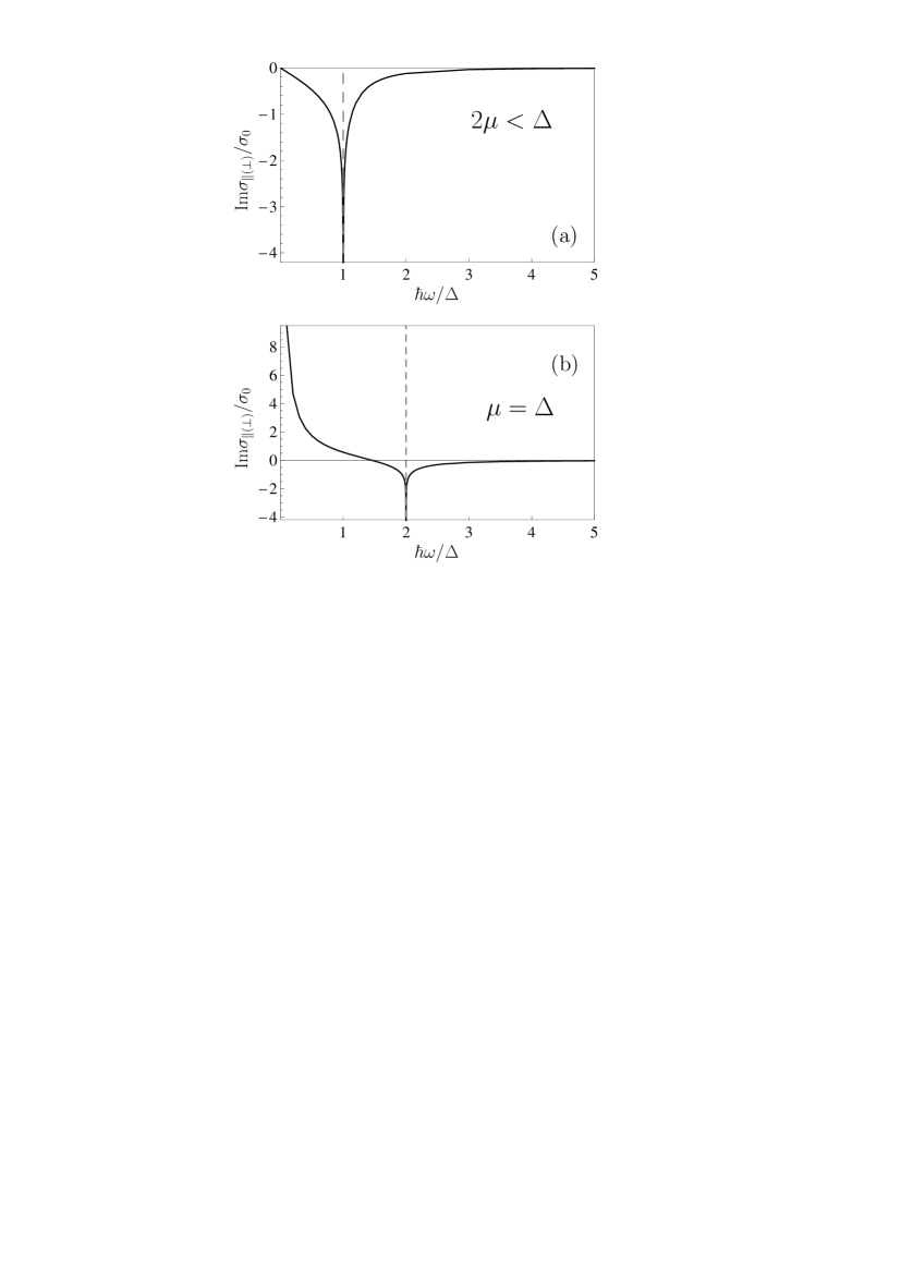
Figure 5: The imaginary part of the conductivity of graphene normalized to the universal conductivity is shown as a function of $\hbar\omega/\Delta$ at zero temperature for (a) any value of the chemical potential satisfying a condition $2\mu<\Delta$ and (b) $\mu=\Delta$.

Now we present the results of numerical computations using Eqs. (55) and (58). In Fig. 5 we plot the imaginary part of the conductivity of graphene normalized to the universal conductivity $\sigma_{0}$ as a function of the dimensionless parameter $\hbar\omega/\Delta$ for (a) $\Delta>2\mu$ and (b) $\Delta=\mu$. In Fig. 5(a) computations have been performed by using Eq. (55). In this case the value of ${\rm Im}\sigma_{\|(\bot)}$ does not depend on a specific value of the chemical potential $\mu$. It is important only that $2\mu<\Delta$. At $\hbar\omega=\Delta$ the imaginary part of the graphene conductivity goes to minus infinity. For $\hbar\omega/\Delta\ll 1$ the imaginary part of conductivity goes to zero by the linear law [see Eq. (59)]. In Fig. 5(b) computations have been performed by using Eq. (58). Here, the value of the chemical potential $\mu=\Delta$ was chosen, i.e., $\Delta<2\mu$. In this case the value of ${\rm Im}\sigma_{\|(\bot)}$ depends essentially on the specific value of $\mu$. For $\hbar\omega/\Delta\ll 1$ the imaginary part of graphene conductivity goes to infinity in accordance with Eq. (60). At $\hbar\omega=2\mu=2\Delta$, i.e., at $\hbar\omega/\Delta=2$, ${\rm Im}\sigma_{\|(\bot)}$ goes to minus infinity.

V Conclusions and discussion

In this paper, we have developed the complete theory of electrical conductivity of graphene with taken into account mass-gap parameter and chemical potential at arbitrary temperature. This was done in the framework of the Dirac model starting from the first principles of quantum electrodynamics at nonzero temperature. The main quantity, used to investigate the conductivity properties of graphene, is the polarization tensor in (2+1)-dimensional space-time. For a gapped graphene with zero chemical potential it was initially found only at the pure imaginary Matsubara frequencies in Refs. 39 ; 40 and in the other form, allowing an analytic continuation to the entire plane of complex frequencies, in Ref. 52 . The polarization tensor of gapped graphene with nonzero chemical potential was presented in Ref. 62 along the imaginary frequency axis. Here, we present the analytic continuation of this tensor to the real frequency axis, which is required for rigorous investigation of the conductivity of graphene. Specifically, we demonstrate that for nonzero chemical potential the temperature-dependent contribution to the polarization tensor at real frequencies does not vanish in the limit of zero temperature and, generally speaking, results in some additional terms depending on both the mass gap and chemical potential.

In the framework of this formalism, the real parts of the in-plane and out-of-plane conductivities of graphene have been found both in the local approximation and with taken into account corrections due to nonlocality. The latter were shown to be of the order of $10^{-5}$ in relation to the main contribution. It was demonstrated that the real parts of the graphene conductivities are not equal to zero only for frequencies exceeding the mass-gap parameter. In this frequency region we have obtained very simple analytic results for the real parts of the conductivity of graphene at both zero and nonzero temperature. In the limit of large frequencies the real part of graphene conductivity goes to the universal conductivity. In several specific cases our results reproduce and generalize the ones obtained earlier in the literature using various approximate and phenomenological approaches. We have also performed numerical computations illustrating the dependence of the conductivity of graphene on the chemical potential.

Furthermore, the imaginary part of the conductivity of graphene has been investigated. It was shown to be nontrivial at all frequencies. In the local limit, the exact expression for the imaginary part of conductivity was obtained, as well as asymptotic limits of this expression for different relationships between the mass gap and chemical potential. In the limiting case of zero temperature, simple analytic results for the imaginary parts of the graphene conductivity were derive, which turned out to be quite different depending on whether the mass gap is smaller or larger than twice the chemical potential. Specifically, it was shown that in the latter case the imaginary part of conductivity goes to minus infinity at the frequency equal to the mass gap. In the former case, the imaginary part of conductivity turns to infinity at zero frequency and to minus infinity at the frequency equal to twice the chemical potential. In the limit of large frequencies the imaginary part of graphene conductivity goes to zero. The numerical computations for the imaginary part of conductivity have been performed at both nonzero and zero temperature to illustrate the obtained results.

The obtained rigorous results for the electric conductivity of graphene can be used as a guide when comparing between different approximate and phenomenological approaches and in the confrontation between experiment and theory.

Appendix A

Here, we derive the asymptotic expressions (49), (51) and (53) for the integral $Y(\omega,T,\Delta,\mu)$ defined in Eq. (48). We consider the limiting case of low temperatures satisfying the condition $k_{B}T\ll\mu$. It is easily seen that under this condition the exponent-containing fractions in Eq. (47) with $\kappa=1$ and $\kappa=-1$, but with positive power of the exponent, can be neglected as compared to the fraction with $\kappa=-1$ and negative power of exponent. The latter occurs under the conditions $\Delta<2\mu$ and $\hbar\omega t<2\mu$. Taking these conditions into account, the upper integration limit in Eq. (47) can be replaced with $2\mu/(\hbar\omega)$.

Now we expand the remaining exponent-containing fraction of Eq. (48) in the powers of exponent with negative argument and obtain

$$Y(\omega,T,\Delta,\mu)=2\int_{\Delta/(\hbar\omega)}^{2\mu/(\hbar\omega)}\!\!\!dt\left[1+\sum_{n=1}^{\infty}(-1)^{n}e^{\frac{n\hbar\omega t}{2k_{B}T}-\frac{n\mu}{k_{B}T}}\right]$$

$$~{}~{}~{}~{}~{}~{}~{}\times\left[1+{\frac{(\hbar\omega)^{2}+\Delta^{2}}{(\hbar\omega)^{2}}}\frac{1}{t^{2}-1}\right].$$ (A1)

After performing the integration of several terms precisely, Eq. (A1) can be rewritten in the form

$$Y(\omega,T,\Delta,\mu)=\frac{4\mu}{\hbar\omega}-\frac{2\Delta}{\hbar\omega}-{\frac{(\hbar\omega)^{2}+\Delta^{2}}{(\hbar\omega)^{2}}}\left(\ln\left|\frac{2\mu+\hbar\omega}{2\mu-\hbar\omega}\right|-\ln\left|\frac{\Delta+\hbar\omega}{\Delta-\hbar\omega}\right|\right)$$

$$~{}~{}+2\sum_{n=1}^{\infty}e^{-\frac{n\mu}{k_{B}T}}(-1)^{n}\int_{\Delta/(\hbar\omega)}^{2\mu/(\hbar\omega)}\!\!\!dte^{\frac{n\hbar\omega t}{2k_{B}T}}\left[1+{\frac{(\hbar\omega)^{2}+\Delta^{2}}{(\hbar\omega)^{2}}}\frac{1}{t^{2}-1}\right].$$ (A2)

The larger contributions to the integral in this equation are given by the larger values of $t$. If we assume in addition that $\hbar\omega\ll 2\mu$, the main contribution to the integral is given by $t\gg 1$. In this case the quantity in the square brackets can be replaced with unity and after the integration one obtains

$$Y(\omega,T,\Delta,\mu)=\frac{4\mu}{\hbar\omega}-\frac{2\Delta}{\hbar\omega}-{\frac{(\hbar\omega)^{2}+\Delta^{2}}{(\hbar\omega)^{2}}}\left(\ln\left|\frac{2\mu+\hbar\omega}{2\mu-\hbar\omega}\right|-\ln\left|\frac{\Delta+\hbar\omega}{\Delta-\hbar\omega}\right|\right)$$

$$~{}~{}+\frac{4k_{B}T}{\hbar\omega}\sum_{n=1}^{\infty}\frac{(-1)^{n}}{n}\left[1-e^{-\frac{n(2\mu-\Delta)}{2k_{B}T}}\right].$$ (A3)

Taking into account the above conditions, we find that an exponential term in the square brackets is much less than unity. Then the summation of the series results in $-\ln 2$, and from (A3) one arrives to Eq. (49).

Now we preserve the condition $\Delta<2\mu$, but, as opposite to the above, assume that $\hbar\omega\gg 2\mu$. In this case $t\ll 1$ over the entire integration region and, thus,

$$\left[1+{\frac{(\hbar\omega)^{2}+\Delta^{2}}{(\hbar\omega)^{2}}}\frac{1}{t^{2}-1}\right]\approx 1-{\frac{(\hbar\omega)^{2}+\Delta^{2}}{(\hbar\omega)^{2}}}=-\frac{\Delta^{2}}{(\hbar\omega)^{2}}.$$ (A4)

Substituting Eq. (A4) in Eq. (A2) and performing the integration and summation in the same way as above, one obtains Eq. (51).

We continue to consider the case of low temperature, $k_{B}T\ll\mu$, but under the opposite condition $\Delta>2\mu$. In this case the powers of exponents with both $\kappa=1$ and $\kappa=-1$ in Eq. (48) are positive. As a result, the main contribution to the integral is given by the smallest $t\sim\Delta/(\hbar\omega)$. Consequently, instead of Eq. (A4) one finds

$$\left[1+{\frac{(\hbar\omega)^{2}+\Delta^{2}}{(\hbar\omega)^{2}}}\frac{1}{t^{2}-1}\right]\approx{\frac{2\Delta^{2}}{\Delta^{2}-(\hbar\omega)^{2}}}.$$ (A5)

Substituting Eq. (A5) in Eq. (48) and expanding both fractions in the powers of exponents with negative arguments, we arrive at

$$Y(\omega,T,\Delta,\mu)=\frac{4\Delta^{2}}{\Delta^{2}-(\hbar\omega)^{2}}\int_{\Delta/(\hbar\omega)}^{\infty}\!\!\!dt\sum_{n=1}^{\infty}(-1)^{n+1}\left(e^{-n\frac{\hbar\omega t+2\mu}{2k_{B}T}}+e^{-n\frac{\hbar\omega t-2\mu}{2k_{B}T}}\right).$$ (A6)

Integration in Eq. (A6) with respect to $t$ leads to

$$Y(\omega,T,\Delta,\mu)=\frac{8k_{B}T}{\hbar\omega}\frac{\Delta^{2}}{\Delta^{2}-(\hbar\omega)^{2}}\sum_{n=1}^{\infty}\frac{(-1)^{n+1}}{n}\left(e^{-n\frac{\Delta+2\mu}{2k_{B}T}}+e^{-n\frac{\Delta-2\mu}{2k_{B}T}}\right).$$ (A7)

Under the above conditions we can restrict ourselves by only the first term of the series in Eq. (A7) which immediately results in Eq. (53).

                      

                      

                      

                      

Figure 4: The imaginary part of the conductivity of graphene normalized to the universal conductivity is shown as a function of the chemical potential at $T=300\,$K for three values of frequency $\hbar\omega=0.01$, 0.05, and 0.099 eV (lines 1, 2, and 3, respectively).

References

- (1) Physics of Graphene, ed. H. Aoki and M. S. Dresselhaus (Springer, Cham, 2014).
- (2) M. I. Katsnelson, Graphene: Carbon in Two Dimensions (Cambridge University Press, Cambridge, 2012).
- (3) A. H. Castro Neto, F. Guinea, N. M. R. Peres, K. S. Novoselov, and A. K. Geim, Rev. Mod. Phys. 81, 109 (2009).
- (4) S. Das Sarma, S. Adam, E. H. Hwang, and E. Rossi, Rev. Mod. Phys. 83, 407 (2011).
- (5) K. Ziegler, Phys. Rev. Lett. 97, 266802 (2006).
- (6) K. Ziegler, Phys. Rev. B 75, 233407 (2007).
- (7) M. Lewkowicz and B. Rosenstein, Phys. Rev. Lett. 102, 106802 (2009).
- (8) A. W. W. Ludwig, M. P. A. Fisher, R. Shankar, and G. Grinstein, Phys. Rev. B 50, 7526 (1994).
- (9) T. Ando, Y. Zheng, and H. Suzuura, J. Phys. Soc. Jpn. 71, 1318 (2002).
- (10) L. A. Falkovsky and A. A. Varlamov, Eur. Phys. J. B 56, 281 (2007).
- (11) T. Stauber, N. M. R. Peres, and A. K. Geim, Phys. Rev. B 78, 085432 (2008).
- (12) T. Stauber, J. Phys.: Condens. Matter 26, 123201 (2014).
- (13) M. Merano, Phys. Rev. A 93, 013832 (2016).
- (14) V. P. Gusynin and S. G. Sharapov, Phys. Rev. B 73, 245411 (2006).
- (15) M. I. Katsnelson, Eur. Phys. J. B 51, 157 (2006).
- (16) N. M. R. Peres, F. Guinea, and A. H. Castro Neto, Phys. Rev. B 73, 125411 (2006).
- (17) V. P. Gusynin, S. G. Sharapov, and J. P. Carbotte, Phys. Rev. Lett. 98, 157402 (2007).
- (18) M. Trushin and J. Schliemann, Phys. Rev. Lett. 99, 216602 (2007).
- (19) L. A. Falkovsky and S. S. Pershoguba, Phys. Rev. B 76, 153410 (2007).
- (20) M. Auslender and M. I. Katsnelson, Phys. Rev. B 76, 235425 (2007).
- (21) V. P. Gusynin and S. G. Sharapov, J. Phys.: Condens. Matter 19, 026222 (2007).
- (22) V. P. Gusynin, S. G. Sharapov, and J. P. Carbotte, Int. J. Mod. Phys. B 21, 4611 (2007).
- (23) N. M. R. Peres and T. Stauber, Int. J. Mod. Phys. B 22, 2529 (2008).
- (24) T. G. Pedersen, A.-P. Jauho, and K. Pedersen, Phys. Rev. B 79, 113406 (2009).
- (25) A. Qaiumzadeh and R. Asgari, Phys. Rev. B 79, 075414 (2009).
- (26) P. K. Pyatkovsky, J. Phys.: Condens. Matter 21, 025506 (2009).
- (27) J. J. Palacios, Phys. Rev. B 82, 165439 (2010).
- (28) N. M. R. Peres, Rev. Mod. Phys. 82, 2673 (2010).
- (29) L. Moriconi and D. Niemeyer, Phys. Rev. B 84, 193401 (2011).
- (30) A. Scholz and J. Schliemann, Phys. Rev. B 83, 235409 (2011).
- (31) P. V. Buividovich, E. V. Luschevskaya, O. V. Pavlovsky, M. I. Polikarpov, and M. V. Ulybyshev, Phys. Rev. B 86, 045107 (2012).
- (32) Á. Bácsi and A. Virosztek, Phys. Rev. B 87, 125425 (2013).
- (33) C. A. Dartora and G. G. Cabrera, Phys. Rev. B 87, 165416 (2013).
- (34) T. Louvet, P. Delplace, A. A. Fedorenko, and D. Carpentier, Phys. Rev. B 92, 155116 (2015).
- (35) D. K. Patel, A. C. Sharma, and S. S. Z. Ashraf, Phys. Status Solidi 252, 282 (2015).
- (36) L. Rani and N. Singh, J. Phys.: Condens. Matter 29, 255602 (2017).
- (37) V. P. Gusynin, S. G. Sharapov, and J. P. Carbotte, New J. Phys. 11, 095013 (2009).
- (38) S. A. Jafari, J. Phys.: Condens. Matter 24, 205802 (2012).
- (39) E. V. Gorbar, V. P. Gusynin, V. A. Miransky, and I. A. Shovkovy, Phys. Rev. B 66, 045108 (2002).
- (40) M. Bordag, I. V. Fialkovsky, D. M. Gitman, and D. V. Vassilevich, Phys. Rev. B 80, 245406 (2009).
- (41) I. V. Fialkovsky, V. N. Marachevsky, and D. V. Vassilevich, Phys. Rev. B 84, 035446 (2011).
- (42) M. Bordag, G. L. Klimchitskaya, and V. M. Mostepanenko, Phys. Rev. B 86, 165429 (2012).
- (43) M. Chaichian, G. L. Klimchitskaya, V. M. Mostepanenko, and A. Tureanu, Phys. Rev. A 86, 012515 (2012).
- (44) G. L. Klimchitskaya and V. M. Mostepanenko, Phys. Rev. B 87, 075439 (2013).
- (45) B. Arora, H. Kaur, and B. K. Sahoo, J. Phys. B 47, 155002 (2014).
- (46) K. Kaur, J. Kaur, B. Arora, and B. K. Sahoo, Phys. Rev. B 90, 245405 (2014).
- (47) G. L. Klimchitskaya and V. M. Mostepanenko, Phys. Rev. A 89, 012516 (2014).
- (48) G. L. Klimchitskaya and V. M. Mostepanenko, Phys. Rev. B 89, 035407 (2014).
- (49) G. L. Klimchitskaya and V. M. Mostepanenko, Phys. Rev. A 89, 052512 (2014).
- (50) G. L. Klimchitskaya and V. M. Mostepanenko, Phys. Rev. A 89, 062508 (2014).
- (51) G. L. Klimchitskaya, V. M. Mostepanenko, and Bo E. Sernelius, Phys. Rev. B 89, 125407 (2014).
- (52) G. L. Klimchitskaya, U. Mohideen, and V. M. Mostepanenko, Phys. Rev. B 89, 115419 (2014).
- (53) M. Bordag, G. L. Klimchitskaya, V. M. Mostepanenko, and V. M. Petrov, Phys. Rev. D 91, 045037 (2015); 93, 089907(E) (2016).
- (54) G. L. Klimchitskaya and V. M. Mostepanenko, Phys. Rev. B 91, 174501 (2015).
- (55) G. L. Klimchitskaya, Int. J. Mod. Phys. A 31, 1641026 (2016).
- (56) V. B. Bezerra, G. L. Klimchitskaya, V. M. Mostepanenko, and C. Romero, Phys. Rev. A 94, 042501 (2016).
- (57) G. Bimonte, G. L. Klimchitskaya, and V. M. Mostepanenko, Phys. Rev. A 96, 012517 (2017).
- (58) G. L. Klimchitskaya, C. C. Korikov, and V. M. Petrov, Phys. Rev. B 92, 125419 (2015); 93, 159906(E) (2016).
- (59) G. L. Klimchitskaya and V. M. Mostepanenko, Phys. Rev. A 93, 052106 (2016).
- (60) G. L. Klimchitskaya and V. M. Mostepanenko, Phys. Rev. B 95, 035425 (2017).
- (61) G. L. Klimchitskaya and V. M. Mostepanenko, Phys. Rev. B 93, 245419 (2016).
- (62) G. L. Klimchitskaya and V. M. Mostepanenko, Phys. Rev. B 94, 195405 (2016).
- (63) M. Bordag, I. Fialkovskiy, and D. Vassilevich, Phys. Rev. B 93, 075414 (2016); 95, 119905(E) (2017).
- (64) A. I. Akhiezer and V. B. Berestetskii, Quantum Electrodynamics (Interscience, New York, 1965).
- (65) S. S. Schweber, An Introduction to Relativistic Quantum Field Theory (Dover, New York, 2005).
- (66) Bo E. Sernelius, Phys. Rev. B 85, 195427 (2012).
- (67) Bo E. Sernelius, J. Phys.: Condens. Matter 27, 214017 (2015).
- (68) A. Schmitt, Dense Matter in Compact Stars: A Pedagogical Introduction (Springer, Berlin, 2010).
- (69) S. Ryu, C. Mudry, A. Furusaki, and A. W. W. Ludwig, Phys. Rev. B 75, 205344 (2007).
- (70) K. F. Mak, M. Y. Sfeir, Y. Wu, C. H. Lui, J. A. Misewich, and T. F. Heinz, Phys. Rev. Lett. 101, 196405 (2008).
- (71) L. A. Falkovsky, J. Phys.: Conf. Series 129, 012004 (2008).
- (72) A. A. Banishev, H. Wen, J. Xu, R. K. Kawakami, G. L. Klimchitskaya, V. M. Mostepanenko, and U. Mohideen, Phys. Rev. B 87, 205433 (2013).