Active Galactic Nuclei Feedback in an Elliptical Galaxy with the most updated AGN physics (I): low-angular momentum case

Abstract

We investigate the effects of AGN feedback on the cosmological evolution of an isolated elliptical galaxy by performing two-dimensional high-resolution hydrodynamical numerical simulations. The inner boundary of the simulation is chosen so that the Bondi radius is resolved. Compared to previous works, the two accretion modes, namely hot and cold, which correspond to different accretion rates and have different radiation and wind outputs, are carefully discriminated and the feedback effects by radiation and wind in each mode are taken into account. The most updated AGN physics, including the descriptions of radiation and wind from the hot accretion flows and wind from cold accretion disks, are adopted. Physical processes like star formation, Type Ia and Type II supernovae are taken into account. We study the AGN light curve, typical AGN lifetime, growth of the black hole mass, AGN duty-cycle, star formation, and the X-ray surface brightness of the galaxy. We compare our simulation results with observations and find general consistency. Comparisons with previous simulation works find significant differences, indicating the importance of AGN physics. The respective roles of radiation and wind feedbacks are examined and it is found that they are different for different problems of interest such as AGN luminosity and star formation. We find that it is hard to neglect any of them, so we suggest to use the names of “cold feedback mode” and “hot feedback mode” to replace the currently used ones.

1. Introduction

There are growing evidences for the co-evolution between the central supermassive black holes and their host galaxies (Kormendy & Ho, 2013), including the strong correlation between the mass of the black hole and the luminosity, stellar velocity dispersion, or the stellar mass in the galaxy spheroid (Magorrian et al., 1998; Tremaine et al., 2002; Häring & Rix, 2004; Gültekin et al., 2009). It is generally believed that AGN feedback plays an important role in the evolution of galaxies and results in the co-evolution between black hole growth and galaxy evolution (Fabian, 2012; Kormendy & Ho, 2013).

Over the past decade many theoretical studies aiming at AGN feedback in galaxy formation and evolution have been performed, especially using the approach of hydrodynamical numerical simulation (e.g. Di Matteo et al., 2005; Springel et al., 2005; Sijacki et al., 2007; Ciotti & Ostriker, 2007; Booth & Schaye, 2009; Ciotti et al., 2010, 2017; Ostriker et al., 2010; Debuhr et al., 2011; Hirschmann et al., 2014; Gan et al., 2014; Eisenreich et al., 2017; Weinberger et al., 2017a). The most serious challenge of these studies is the large dynamical range: a proper simulation involving both the large-scale structure of the universe and the black hole accretion scales would require a spatial range of over ten orders of magnitude, from the black hole radius ($R_{s}$) of $\sim 10^{-5}\,{\rm pc}$ for a $10^{8}M_{\odot}$ mass black hole, to a scale of hundreds of Mpc. This is still technically infeasible even with modern supercomputers. Consequently, if the study focuses mainly on large scales, such as the galaxy or larger scales, as it is the case for most AGN feedback works so far, since the scale of black hole accretion cannot be resolved, so-called sub-grid models have to be used. This “sub-grid” model means that some simplifications and approximations are used when describing the black hole accretion and its outputs.

The first issue the “sub-grid” model needs to deal with is the determination of the mass accretion rate of the central black hole. The exact determination of the mass accretion rate is crucial for the study of AGN feedback since it determines the strength of the AGN outputs such as radiation, jet, and wind. Most works adopt the Bondi solution (Bondi, 1952; Frank et al., 2002) to calculate the mass accretion rate (e.g., Springel et al. 2005; Booth & Schaye 2009; McCarthy et al. 2010, 2017; Choi et al. 2012, 2015; Le Brun et al. 2014; Schaye et al. 2015; see recent review by Negri & Volonteri 2017). But this approach suffers from the following problems. First, the accretion gas is usually turbulent and inhomogeneous (e.g, Gaspari et al., 2013). Second, the Bondi solution neglects the angular momentum of the gas (Hopkins & Quataert, 2011; Tremmel et al., 2017). Perhaps the most serious problem is that, since the Bondi radius cannot be resolved, some form of extrapolations to the density and temperature have to be used. This is in practice achieved by introducing a constant “accretion rate boost parameter $\alpha$” with a typical value of 100 (e.g., Springel et al., 2005). The underlying idea is that at large radii, the density may be underestimated while the temperature overestimated compared to the values at the Bondi radius, so the accretion rate will be underestimated. Obviously, the value of $\alpha$ has very large uncertainties. In fact, different works choose quite different values, from $\alpha\sim 1$ to $\sim 300$ (e.g., Booth & Schaye, 2009). Most recently, taking the AGN feedback in an isolated galaxy as an example, Negri & Volonteri (2017) carefully studied how well the Bondi approximation describes the mass accretion rate. They have performed many runs with different resolutions using the Bondi approximation, and compared these results with a high-resolution run which can well resolve the Bondi radius thus precisely determining the accretion rate. They find that approximated Bondi formalism can lead to both over- and underestimations of the black hole growth, depending on the resolution and how the variables entering into the formalism are calculated. So how to determine the mass accretion rate of the central AGN is still an unsolved problem.

In this paper, we focus on discussing another aspect of the “sub-grid” model. That is, for a given mass accretion rate, what will be the exact outputs, i.e., radiation, wind, and jet, from the AGN? In many large-scale cosmological simulation works, once they estimate the mass accretion rate, they estimate the total energy output of the accretion flow and then simply assume some fraction of these energy is converted into the thermal energy of the surrounding ISM (e.g., Booth & Schaye, 2009), except in some recent works in which the importance of mechanical feedback by wind has been recognized and taken into account (e.g., Choi et al., 2015; Weinberger et al., 2017a, b; Gaspari & Sa̧dowski, 2017). In reality, however, the output of black hole accretion is much more complicated. As we will discuss in detail in §2, there are two kinds of accretion modes, namely cold and hot, and in each mode the three types of outputs are quite different. In the best cases, the two different accretion (feedback) modes are discriminated, but the most updated accretion physics describing their outputs in each mode has not been properly taken into account. This is especially the case for the hot accretion mode, in which case much progress has been made in recent several years. For example, when calculating the Compton heating, usually the same Compton temperature value is used for both accretion modes. This is not correct because the typical spectrum emitted in the two modes is different (Xie et al. 2017; see also §2 below). The properties of wind in the two modes are also often described by the same parameterized way, while in recent couple of years the properties of wind launched from the hot accretion flow have been intensively studied and well understood, which is found to be very different from the wind from cold accretion disks (see §2 below for details).

By performing two-dimensional hydrodynamical numerical simulations, we in this paper study the evolution of an isolated elliptical galaxy. The inner boundary is chosen to resolve the Bondi radius so that the mass accretion rate can be calculated precisely. We consider two accretion modes, in each mode we consider both the radiation and wind. Jets are neglected as we will explain later in this paper. Heating and cooling, star formation, Type Ia and Type II supernovae are included in the simulation. These features are the same as those of some previous works (e.g., Novak et al., 2011; Ciotti & Ostriker, 2012; Gan et al., 2014; Negri & Volonteri, 2017; Ciotti et al., 2017). However, different from these previous works, in this paper we will adopt the most recent progresses in AGN physics which give correct descriptions of radiation and wind. As we will see in §2, these progresses are especially in the regime of hot accretion flows but also in the description of wind from cold accretion disk.

The paper is organized as follows. In §2, we present the most updated AGN physics we use in the simulation. The other physics of the model and the details of the model setup are described in §3. The results of the simulation, namely the effects of the AGN feedback in the galaxy evolution, are described in detail in §4. We will also compare our results with those obtained in previous works to investigate the effects of the AGN physics. Attention will be also paid on the respective roles of radiative and mechanical feedback. The last section is devoted to a summary and conclusion. As the first paper of a series in this project, in this work we assume the specific angular momentum of the gas in the galaxy is low. In a following paper (Yoon et al., 2018), we will investigate the effect of AGN feedback on the evolution of elliptical galaxies with a high specific angular momentum.

2. The AGN physics

As in previous works, the feedback effects are considered by injecting radiation and wind launched by the AGN in the innermost grids of the simulation domain. The subsequent interaction of radiation and wind with the ISM in the galaxy is self-consistently calculated. In this section, we describe in detail how the properties of radiation and wind are calculated for a given accretion rate. This AGN physics is also often called “feedback physics” or “sub-grid physics” in literature. We emphasize that the most recent progresses in the field of AGN study will be taken into account.

2.1. The accretion rate and two accretion modes

Since our simulation can resolve the Bondi radius, we can calculate the accretion rate at that radius directly. Note that we should not put an additional constraint of “Eddington limit” to the mass accretion rate as in some papers. The Eddington limit only applies for a pure spherical accretion which is almost always an oversimplification when we consider accretion flow close to the black hole. Once the accretion flow has some angular momentum, the accretion rate can be of any value.

Then our question is, for a given accretion rate, what will be the output of AGN, i.e., what are the properties of emitted radiation and wind?

After several decades’ efforts, tremendous progresses have been made in the theory of black hole accretion (see reviews by Pringle, 1981; Frank et al., 2002; Blaes, 2014; Yuan & Narayan, 2014). We know that according to the temperature of the accretion flow, we have two series of solutions, i.e., cold (e.g., the standard thin disk; Shakura & Sunyaev (1973)) and hot (e.g., the advection-dominated accretion flow; Narayan & Yi (1995)). Mathematically, these two series of solutions have a large overlap in terms of the corresponding accretion rate. In other words, for a given accretion rate, both the cold and hot accretion solutions are available for some accretion rates (Narayan & Yi, 1995; Yuan & Narayan, 2014). Fortunately, such a theoretical degeneracy is broken by our observations of black hole X-ray binaries. Black hole X-ray binaries come in two main “states” – soft and hard states – which are described by the standard thin disk and the hot accretion flow, respectively. During the decay phase of an outburst of a black hole X-ray binary, the luminosity decreases with time. It is interesting to note that the source always transits from the soft to the hard state once the luminosity passes through a critical luminosity

$$L_{\rm c}\approx 2\%L_{\rm Edd}$$ (1)

(McClintock & Remillard, 2006). In other words, we never observe a soft state with $L_{\rm BH}\lesssim 2\%L_{\rm Edd}$. So this “critical” luminosity is a boundary set by nature between the cold and hot accretion flows.

We have the almost same situation in the case of AGNs since the accretion physics does not depend on the mass of the black hole. For AGNs, we now know that luminous AGNs such as quasars correspond to the soft state, and are described by the cold accretion flow. In this accretion mode, accretion flow produces radiation and wind but not jet. Low-luminosity AGNs correspond to the hard state and are described by hot accretion flows (Ho, 2008; Yuan & Narayan, 2014). In this accretion mode, accretion flow produces three kinds of output, namely radiation, wind, and jet (Yuan & Narayan, 2014).

The output from the two modes of accretion is quite different and this obviously will determine the different feedback effects. In the literature of AGN feedback, the corresponding feedback are called quasar (or radiative) and radio (or kinetic, or maintenance, or jet) modes, respectively. The names of the two feedback mode are not only diverse, but also confusing. They were invented perhaps to emphasize the dominance of some forms of AGN output in an accretion mode, for example the radiation in the cold accretion mode and the jet in the hot accretion mode. However, as we can see from §2.4, it is not obvious why we can neglect the other forms of output in a given accretion mode, e.g., the wind output in the cold accretion mode and the radiation output in the hot accretion mode, at least when we compare the energy and momentum fluxes of various AGN outputs (wind and radiation). It is even on the opposite with what we think if we consider the feedback effects. For example, in the quasar mode, at least in terms of controlling the black hole growth, wind feedback is much more important than radiation (§4.3). While in the radio mode, when the accretion rate is low, radiative feedback seems to be at least equally important with wind in controlling the accretion rate of the black hole (§4.2). Therefore, in this paper, we suggest to simply follow the names of black hole accretion mode and replace these complicated feedback names by “cold feedback mode” and “hot feedback mode”, representing the feedback occurred in the two accretion modes respectively.

The mass accretion rate corresponding to the critical luminosity $L_{\rm c}$ is:

$$\dot{M}_{\rm c}\approx\frac{L_{\rm c}}{\epsilon_{\rm EM,cold}c^{2}}.$$ (2)

Here $\epsilon_{\rm EM,cold}$ is the radiative efficiency of a cold accretion disk. Note that this accretion rate is the rate at the innermost region of the accretion disk where most of the radiation comes from. Since winds exist in a cold disk, the accretion rate at the Bondi radius must be larger than this rate. For our description of wind launched from a cold disk (refer to §2.2.2), the ratio of accretion rate close to the black hole and the wind mass flux is a weak function of accretion rate. For typical parameters of our model, the ratio is close to unity, i.e., $\dot{M}_{\rm BH}\approx\dot{M}_{\rm W}$. So the accretion rate at the innermost radius of the simulation domain ($r_{\rm in}$) is only 2 times of that close to the black hole horizon. Therefore, in our simulation, we compare the accretion rate at $r_{\rm in}$ (calculated by Eq. 50) with $\dot{M}_{\rm c}$ in Eq. (2) to decide which accretion mode the accretion flow should choose. In the next two subsections, we describe the output from the cold and hot accretion modes. In this work, we neglect the effect of jet because we assume that for the feedback study of a single galaxy as in the present work, the jet may simply pierce through the galaxy and has negligible interaction with the galaxy since it is well collimated, although it should be important for the evolution of large scale structure such as galaxy clusters. But we note that there are debates on this topic (e.g., see Gaibler et al. (2012) for a different opinion) so it is necessary to examine this assumption in the future works.

2.2. Cold accretion (feedback) mode

2.2.1 The accretion within the Bondi radius

Our simulation can resolve the Bondi radius, which is the outer boundary of the accretion flow. But within Bondi radius, the accretion onto the black hole still cannot be resolved and must be treated as “sub-grid” physics. The dynamics of accretion gas within Bondi radius is likely complicated and is a good project of future research. In this work, we assume the following simple scenario. Since the specific angular momentum of the gas is low, the gas will first freely fall until a small accretion disk is formed with the size of the circularization radius. Note that the disk should gradually grow with time because of the angular momentum transport of the accretion flow(Bu & Yuan, 2014). Wind will be launched from the disk and will affect the black hole accretion rate. In the following we estimate the black hole accretion rate according to the above scenario. The approach is largely adopted from Ciotti & Ostriker (2012) but with some modifications.

The mass accretion rate at the innermost radial grid ($\dot{M}(r_{\rm in})$) of our simulation is calculated by Eq. (50). The infall timescale from $r_{\rm in}$ is calculated by

$$\tau_{\rm ff}=\frac{\rm r_{in}}{v_{\rm ff}},~{}~{}~{}v_{\rm ff}\equiv\left(\frac{2\,GM_{\rm BH}}{r_{\rm in}}\right)^{1/2},$$ (3)

where $\tau_{\rm ff}$ and $\,v_{\rm ff}$ are free-fall time scale and velocity at the inner-most grid $r_{\rm in}$. The effective accretion rate at which gas feeds the small accretion disk is then obtained from

$$\frac{d\,\dot{M}^{\rm eff}}{d\,t}=\frac{\dot{M}(r_{\rm in})-\dot{M}^{\rm eff}}{\tau_{\rm ff}}.$$ (4)

This equation implies that when $\dot{M}(r_{\rm in})$ drops to zero the small accretion disk experiences a fueling declining exponentially with time. Given our fiducial numerical set-up (i.e. $R_{\rm in}$=2.5 pc and $M_{\rm BH,init}\sim 10^{9}\,M_{\odot}$), the free-fall time is $\tau_{\rm ff}\sim 10^{3}$ yr.

Once the gas reaches the circularization radius, $R_{\rm cir}$, it forms an accretion disk and fuels the black hole with the accretion (viscous) timescale. With the computed total mass of the gas in the disk, $M_{\rm dg}$, the mass inflow rate at $R_{\rm cir}$ in the disk can be estimated as

$$\dot{M}_{\rm d,inflow}=\frac{M_{\rm dg}}{\tau_{\rm vis}},$$ (5)

where $\tau_{\rm vis}$ is the instantaneous viscous timescale at $R_{\rm cir}$, which is described in Kato et al. (2008),

$$\tau_{\rm vis}\approx 1.2\times 10^{6}\,{\rm yr}\left(\frac{\alpha}{0.1}\right)^{-1}\left(\frac{R_{\rm cir}}{100\,r_{\rm s}}\right)^{7/2}\left(\frac{M_{\rm BH}}{10^{9}\,M_{\odot}}\right),$$ (6)

where we set the viscosity parameter to $\alpha=0.1$. We note that in the simulation, we set $R_{\rm cir}$ as a free parameter and adopt the value of $R_{\rm cir}=100\,r_{\rm s}$, where $r_{\rm s}\equiv 2GM_{\rm BH}/{c^{2}}$ is the Schwarzschild radius. In this way, the growth of $R_{\rm cir}$ with time is absorbed in this parameter.

While the gas approaches the central black hole via the accretion disk, a fraction of the gas is ejected as a form of wind. So the final black hole mass accretion rate can be obtained from

$$\dot{M}_{\rm BH}=\dot{M}_{\rm d,inflow}-\dot{M}_{\rm W,C},$$ (7)

where $\dot{M}_{\rm W,C}$ is the wind mass flux at the cold accretion disk(see eq. (9)). We will discuss the wind model in §2.2.2.

The total amount of disk gas mass, $M_{\rm dg}$, evolves as

$$\frac{d\,M_{\rm dg}}{d\,t}=\dot{M}^{\rm eff}-\dot{M}_{\rm BH}-\dot{M}_{\rm W,C}.$$ (8)

Combining eqs.(5)-(8), we can estimate the black hole accretion rate $\dot{M}_{\rm BH}$. We note that if the disk is in hot accretion mode, the viscosity time scale is many orders of magnitudes shorter than that in the cold mode. So both $\tau_{\rm ff}$ and $\tau_{\rm vis}$ are very small. Hence, we simply ignore the above-mentioned time lag effects.

2.2.2 Wind

Cold accretion disk can produce strong winds, which have been widely observed in luminous AGNs (e.g., Crenshaw et al., 2003; Tombesi et al., 2010, 2014; King & Pounds, 2015; Liu et al., 2015) and black hole X-ray binaries (e.g., Neilsen & Homan 2012; Homan et al. 2016, see review by Díaz Trigo & Boirin 2016). Three mechanisms have been proposed to explain the production of wind, namely thermal, radiation, and magnetic ones. Debates still exist for which one is the dominant mechanism in various conditions. In principle by performing numerical simulations we could combine all these three mechanisms to calculate the wind properties. Unfortunately, it is still infeasible due to the technical difficulties of globally simulating a thin disk.

Therefore we will obtain the properties of wind to be used in the current work from observations. Some parameters of wind have been measured, such as the velocity, although the value is diverse. Recently, Gofford et al. (2015) have analysed a sample of 51 Suzaku-observed AGNs and presented the properties of wind as a function of the bolometric luminosity of AGNs. Their results indicate that more luminous AGN tends to harbour faster and more energetic winds. In this paper, we adopt the fitted formulas presented in that work to describe the wind. The mass, momentum and energy fluxes of the winds are described by,

$$\dot{M}_{\rm W,C}=0.28\,\,\left(\frac{L_{\rm BH}}{10^{45}\,\rm erg\,s^{-1}}\right)^{0.85}M_{\odot}\,{\rm yr^{-1}},$$ (9)

$$\dot{P}_{\rm W,C}=\dot{M}_{\rm W,C}\,v_{\rm W,C},$$ (10)

$$\dot{E}_{\rm W,C}=\frac{1}{2}\,\dot{P}_{\rm W,C}\,v_{\rm W,C}.$$ (11)

Here $L_{\rm BH}$ is the bolometric luminosity of the AGN. The velocity of wind is described by,

$$v_{\rm W,C}=2.5\times 10^{4}\,\,\left(\frac{L_{\rm BH}}{10^{45}\,\rm erg\,s^{-1}}\right)^{0.4}{\rm km\,s^{-1}}.$$ (12)

An upper limit of $10^{5}{\rm km\,s^{-1}}$ is adopted since observations indicate a saturation of the wind velocity at this value (Gofford et al., 2015).

In the literature, observed value of wind velocity are quite diverse, from the very large value for ultra-fast outflow to the small value for molecular outflows(e.g., Crenshaw et al., 2003; Blustin et al., 2007; Hamann et al., 2008; Tombesi et al., 2010). This is likely because the winds are detected at different distances from the black hole: the wind velocity is larger at smaller distance. The diversity of wind mass flux is possibly also because of the different detection locations. Specifically, the mass flux of wind increases with distance because of mass entrainment of the interstellar medium during the outward propagation of wind. In the observations of Gofford et al. (2015) the winds are detected at a distance of $\sim 10^{2-4}r_{s}$ from the black hole. The innermost grid in our simulation is 2.5 pc (refer to §3.5), which corresponds to $\sim 10^{4}r_{s}$ for a typical black hole mass of $2\times 10^{9}M_{\odot}$ in our simulations. So our adoption of the observational results of Gofford et al. (2015) is justified.

Eq. (9) can be rewritten as

$$\dot{M}_{\rm W,C}=0.28\,\left(\frac{L_{\rm BH}}{L_{\rm Edd}}\right)^{0.85}\left(\frac{L_{\rm Edd}}{10^{45}\,\rm erg\,s^{-1}}\right)^{0.85}\,M_{\odot}\,{\rm yr^{-1}}.$$ (13)

For the Eddington ratio of $l\equiv L_{\rm BH}/L_{\rm Edd}=0.1$ and black hole mass of $M_{\rm BH}=10^{9}\,M_{\odot}$, the mass flux of wind is $\dot{M}_{W,C}\approx 2.5\,{M}_{\odot}\,{\rm yr^{-1}}$. This is quite similar to the mass accretion rate of the black hole, which is $\dot{M}_{\rm BH}=0.1\dot{M}_{\rm Edd}\approx 2\,{M}_{\odot}\,{\rm yr^{-1}}$. From eq. (11), the power of wind is $\dot{E}_{W,C}=0.02\,\dot{M}_{\rm BH}\,c^{2}$. This is five times smaller than the bolometric luminosity, which is $L_{\rm BH}=0.1\dot{M}_{\rm BH}c^{2}$.

The above settings of wind properties are different from previous works (e.g. Novak et al., 2011; Gan et al., 2014; Ciotti et al., 2017). In these works, the wind velocity is usually set to be a constant value of $v_{\rm W}=10^{4}\,{\rm km\,s^{-1}}$, while the mass flux or the power of wind is usually described by a parameter called mechanical efficiency ($\epsilon_{\rm W}$), which is defined as the fraction of mechanical power of wind in the total accretion power. The value of $\epsilon_{W}$ is highly uncertain, its scaling with luminosity is qualitatively similar to but quantitatively different from what we have just introduced above. Typically, the wind power described by the above formula is much stronger than that adopted in previous works.

The next question is the spatial (angular) distribution of the mass flux of wind. In reality, most of mass flux may concentrate close to the surface of the accretion disk. Since our galaxy model is almost spherically symmetric, and since the relative orientation of the accretion disk and the galactic disk is random(Schmitt et al., 2001), the exact description of distribution of wind flux may be not so important so we simply adopt the same description as in previous works (e.g., Novak et al., 2011; Gan et al., 2014; Ciotti et al., 2017). According to this description, the mass flux of wind $\propto{\rm cos}^{2}(\theta)$. Thus, the half-opening angle enclosing half of the mechanical energy is $\approx 45^{\circ}$, and most of the flux concentrates close to the rotation axis of the accretion disk.

2.2.3 Radiation

Since the mass flux of wind is similar to the mass accretion rate of the black hole, the radiation output from the thin disk can be approximated as,

$$L_{\rm BH}=\epsilon_{\rm EM,cold}\dot{M}_{\rm BH}c^{2}$$ (14)

Here $\dot{M}_{\rm BH}$ is the accretion rate close to the black hole calculated by eq. (7). For a cold thin disk, the radiative efficiency $\epsilon_{\rm EM,cold}$ is only a function of black hole spin. In this work we usually set

$$\epsilon_{\rm EM,cold}=0.1,$$ (15)

which means that we assume the black hole is moderately spinning (Wu et al., 2013). To examine the effect of stronger radiation, sometimes we also consider the case of $\epsilon_{\rm EM,cold}\approx 0.3$, which corresponds to a rapidly spinning black hole.

The emitted spectrum in the cold accretion mode is represented by the observed multi-waveband spectrum of quasars. The radiation carries with them energy and momentum. It will heat the ISM via photoionization and Compton scattering. It will also be able to push the gas via electron scattering and photoionization. The radiative heating and cooling we consider in this work are computed using the formulae presented in Sazonov et al. (2005), which describe the net heating and cooling per unit volume of the gas in photoionization equilibrium. It includes Compton heating/cooling, bremsstrahlung cooling, photoionization, and line and recombination cooling. The Compton heating/cooling is usually calculated in terms of “Compton temperature”,

$$H_{\rm Compton}=4.1\times 10^{-35}n^{2}\xi(T_{C}-T)~{}{\rm erg~{}cm^{-3}s^{-1}},$$ (16)

where $\xi=4\pi L_{\rm BH}/n$ is the ionization parameter, $F$ is the flux of photoionizing photons, $n$ is the number density of the ISM, $T$ is the temperature of the ISM, $T_{C}$ is the Compton temperature of the photons, which physically means the energy-weighted average photon energy of the radiation emitted by the AGN. For the cold feedback mode, it can be calculated from the observed spectrum of quasars (Sazonov et al., 2004). The result is

$$T_{\rm C,cold}=2\times 10^{7}{\rm K}.$$ (17)

2.3. Hot accretion (feedback) mode

Compared with the cold mode, the hot accretion mode corresponds to lower accretion rates(Yuan & Narayan, 2014), so both the radiation and the wind emitted from this mode are weaker than those from the cold mode, as shown by Fig. 1. But the hot mode feedback is still potentially very important. This is because, compared to the cold mode, the central AGNs reside in the hot mode for a much longer time than in the cold mode (e.g., Greene & Ho 2007; Figs. 3 & 10 of the present work). So we expect to have an important cumulative effect for the feedback in the hot mode.

2.3.1 Geometry configuration of accretion flow

Before we discuss the radiation and wind in the hot accretion mode, we first need to discuss the geometry of the accretion flow when the accretion rate at the Bondi radius is smaller than $\dot{M}_{\rm c}$ (Eq. (2)). This issue has been well studied in the cases of the hard state of black hole X-ray binaries and low-luminosity AGNs (see Yuan & Narayan, 2014, for a review). The result is that at large radii, the accretion flow is in the form of thin disk; but at a certain radius, $r_{\rm tr}$, the thin disk will be truncated and transits into a hot accretion flow. The value of the transition radius $r_{\rm tr}$ can be described by (Liu et al. 1999; Manmoto & Kato 2000; Gu & Lu 2000; Yuan & Narayan 2004; see review by Yuan & Narayan 2014)

$$r_{\rm tr}=3r_{s}\left[\frac{2\times 10^{-2}\dot{M}_{\rm Edd}}{\dot{M}(r_{\rm in})}\right]^{2}.$$ (18)

Here $\dot{M}(r_{\rm in})$ is the accretion rate at the innermost grid $r_{\rm in}$ of simulation calculated by eq. (50). The transition radius will be small if $\dot{M}(r_{\rm in})$ is large. The largest value of $r_{\rm tr}$ is set to be $r_{\rm in}$.

2.3.2 Wind

The status of study of wind from hot accretion flows is quite different from the case of a cold accretion disk. In this case, the observational data is much fewer compared to the case of cold disk. This is mainly because the gas in the wind from a hot accretion flow is very hot thus generally fully ionized. So it is very difficult to detect them by the usual absorption-line spectroscopy. But still, in recent years, we have gradually accumulated more and more observational evidences for wind from low-luminosity sources in which we believe a hot accretion flow is operating, including low-luminosity AGNs and radio galaxies (e.g., Crenshaw & Kraemer, 2012; Tombesi et al., 2010, 2014; Cheung et al., 2016), the supermassive black hole in our Galactic center, Sgr A* (Wang et al., 2013), and the hard state of black hole X-ray binaries (e.g., Homan et al., 2016). In contrast to the rarity of observational results, we have much better theoretical understanding to the wind launched from hot accretion flows, mainly attributed to the rapid development of numerical simulations in recent years (Yuan et al., 2012; Narayan et al., 2012; Li et al., 2013; Yuan et al., 2015; Bu et al., 2016). This is also partly because radiation is in general dynamically not important in hot accretion flow, and technically it is easy to simulate a hot accretion flow since it is geometrically thick. Especially, the detailed properties of wind from a hot accretion flow have been carefully studied in Yuan et al. (2015) based on three-dimensional general relativity MHD simulation data. In this work, to discriminate the turbulent outflow from real wind, a “virtual particle trajectory” approach has been proposed. Compared to the streamline approach often used in literature, this new approach can give a much more reliable calculation to the mass flux of wind. In the present work, we will use the results obtained by Yuan et al. (2015). We briefly summarize the most relevant results as follows.

We assume that the mass accretion rate at the innermost radius of the simulation domain $\dot{M}(r_{\rm in})$ is roughly equal to the accretion rate at the outer boundary of the hot accretion flow $\dot{M}(r_{\rm tr})$. The outer truncated thin disk should also be able to produce wind, but in this paper we neglect this part of wind. In this case, the accretion rate close to the black hole horizon, which determines the emitted luminosity, is described by (Yuan et al., 2015):

$$\dot{M}_{\rm BH,hot}=\dot{M}(r_{\rm tr})\left(\frac{3r_{s}}{r_{\rm tr}}\right)^{0.5}\approx\dot{M}(r_{\rm in})\left(\frac{3r_{s}}{r_{\rm tr}}\right)^{0.5}.$$ (19)

So the mass flux of wind launched from the hot accretion flow is described by

$$\dot{M}_{\rm W,H}\approx\dot{M}(r_{\rm in})\left[1-\left(\frac{3r_{s}}{r_{\rm tr}}\right)^{0.5}\right].$$ (20)

Compared to jets, the opening angle of wind is much larger (refer to Fig. 1 in Yuan et al. 2015), which makes the interaction between wind and ISM very efficient. According to the detailed analysis by Yuan et al. (2015) (refer to their Fig. 3), the mass flux of wind is distributed within $\theta\sim 30^{\circ}-70^{\circ}$ and $\theta\sim 110^{\circ}-150^{\circ}$ above and below the equatorial plane respectively. Since the hot accretion flow occupies roughly $\theta\sim 70^{\circ}-110^{\circ}$, such a distribution implies that the wind is along the surface of the hot accretion flow. Within the above-mentioned two ranges of $\theta$ angle, the mass flux of wind is assumed to be independent of $\theta$.

The speed of wind when they just leave the transition radius $r_{\rm tr}$ is $v_{\rm W,H}\approx 0.2v_{\rm K}(r_{\rm tr})$ (refer to Eq. (7) in Yuan et al. 2015). Here $v_{\rm K}(r_{\rm tr})$ is the Keplerian velocity at the transition radius $r_{\rm tr}$. When the wind propagates outward, gravitational force will decelerate it, while gradient force of gas pressure and magnetic force will accelerate it. The overall result is that the poloidal velocity of wind roughly keeps constant, and its value can be approximated as (Yuan et al. 2015, Eq. (8); Cui, Yuan & Li 2018, in preparation):

$$v_{\rm W,H}\approx(0.2-0.4)v_{\rm K}(r_{\rm tr}).$$ (21)

In this paper we adopt $v_{\rm W,H}=0.2v_{\rm K}(r_{\rm tr})$. The fluxes of energy and momentum of wind are described by

$$\dot{E}_{\rm W,H}=\frac{1}{2}\dot{M}_{\rm W,H}v_{\rm W,H}^{2},$$ (22)

$$\dot{P}_{\rm W,H}=\frac{2\dot{E}_{\rm W,H}}{v_{\rm W,H}}.$$ (23)

The properties of wind described above are quite different from those adopted in previous works (e.g., Novak et al., 2011; Gan et al., 2014; Ciotti et al., 2017). In these previous works, the velocity of wind is usually set to be a value with reference to the observations of wind in the cold mode. The mass flux or the power of wind in the hot feedback mode are again determined by the “mechanical efficiency” parameter $\epsilon_{W}$. Its value is now much more uncertain, because observational constrains to wind in the hot mode are not good. So usually in these works the wind parameters and their scaling with luminosity are assumed to be the same as those in the cold mode. Consequently, we find that the wind power we adopt in the present work is much stronger than that in previous works. This causes significant differences of simulation results, as we will describe later in this paper.

2.3.3 Radiation

The radiation output from hot accretion flows has been well studied (see Yuan & Narayan, 2014, for a review). Different from a thin disk, the radiative efficiency not only depends on the black hole spin, but more importantly on the accretion rate. The radiative efficiency as a function of accretion rate has been investigated by Xie & Yuan (2012). They fit their numerical calculation results of efficiency by a piecewise power-law function of accretion rate,

$$\epsilon_{\rm EM,hot}(\dot{M}_{\rm BH})=\epsilon_{0}\left(\frac{\dot{M}_{\rm BH}}{0.1L_{\rm Edd}/c^{2}}\right)^{a},$$ (24)

where the values of $\epsilon_{0}$ and $a$ are given in Table 1 of Xie & Yuan (2012). For convenience, we copy their results here,

$$(\epsilon_{0},a) = \left\{\begin{array}[]{ll}(0.2,0.59),&\dot{M}_{\rm BH}/\dot{M}_{\rm Edd}\lesssim 9.4\times 10^{-5}\\ (0.045,0.27),&9.4\times 10^{-5}\lesssim\dot{M}_{\rm BH}/\dot{M}_{\rm Edd}\lesssim 5\times 10^{-3}\\ (0.88,4.53),&5\times 10^{-3}\lesssim\dot{M}_{\rm BH}/\dot{M}_{\rm Edd}\lesssim 6.6\times 10^{-3}\\ (0.1,0),&6.6\times 10^{-3}\lesssim\dot{M}_{\rm BH}/\dot{M}_{\rm Edd}\lesssim 2\times 10^{-2}\end{array}\right.$$ (29)

Here $\dot{M}_{\rm Edd}\equiv 10L_{\rm Edd}/c^{2}$ is the Eddington accretion rate. Note that the calculation of Xie & Yuan (2012) is for a Schwarzschild black hole. Since in the present paper we assume that the black hole is moderately spinning, we multiply $\epsilon_{0}$ in Xie & Yuan (2012) by a factor of $0.1/0.057$. As shown by Xie & Yuan (2012), the radiative efficiency quickly (and of course also luminosity) increases with the accretion rate, and finally becomes almost equal to the efficiency of a thin disk at the highest accretion rate of the hot accretion flow, i.e., the “boundary accretion rate” between the hot and cold modes, as shown by Fig. 1.

The spectrum emitted from a hot accretion flow is quite different from that from a cold thin disk, e.g., the lack of the big-blue-bump which is present in the typical spectrum of quasars (Ho, 1999, 2008). For a given luminosity, the spectrum from a hot accretion flow will have more hard photons compared to that from a cold disk. This makes the radiative heating to ISM via Compton scattering in the hot mode more effective than in a cold mode for the same luminosity. Xie et al. (2017) recently studied this problem in detail and calculated the Compton temperature based on the spectral energy distribution of low-luminosity AGNs combined from literature. The result is

$$T_{\rm C,hot} = \left\{\begin{array}[]{ll}10^{8}\,{\rm K},&10^{-3}\lesssim L_{\rm BH}/L_{\rm Edd}\lesssim 0.02\\ 5\times 10^{7}\,{\rm K}.{}{}&L_{\rm BH}/L_{\rm Edd}\lesssim 10^{-3}\end{array}\right.$$ (32)

This is several times higher than $T_{\rm C,cold}$. This value is smaller than that adopted in Gan et al. (2014), in which they adopt $T_{\rm C,hot}=10^{9}{\rm K}$ by simple estimation.

2.4. Comparison of energy and momentum fluxes of wind and radiation in cold and hot modes

$\begin{array}[]{cc}\includegraphics[width=195.12767pt]{powercomp.pdf}&\includegraphics[width=195.12767pt]{momfluxcomp.pdf}\end{array}$

Figure 1.— The comparison of the power (left) and momentum flux (right) of wind (orange lines) and radiation (blue lines) from hot (solid lines) and cold (dashed lines) accretion modes of AGNs. For comparison, the power and momentum flux of radiation and wind from Gan et al. (2014) are also shown by the dot-dashed lines.

We now compare the fluxes of energy and momentum of wind and radiation in both cold and hot feedback modes. For the cold feedback mode, the energy and momentum fluxes of radiation can be obtained by Eq. (14) and $L_{\rm BH}/c$, respectively. The energy and momentum fluxes of wind can be calculated from eqs. (11) and (10). For the hot feedback mode, the energy and momentum fluxes of wind can be calculated from eqs. (22) & (23). The wind velocity $v_{\rm W,H}$ can be obtained from eq. (21) while the value of transition radius $r_{\rm tr}$ can be obtained by combining eqs. (18) & (50). The energy and momentum fluxes of radiation are $L_{\rm BH}=\epsilon_{\rm EM,hot}\dot{M}_{\rm BH}c^{2}$ and $L_{\rm BH}/c$, respectively. The value of $\epsilon_{\rm EM,hot}$ can be calculated from eqs. (24) & (29).

The results of such a comparison are shown in Fig. 1. The left and right panels denote the power and momentum fluxes, respectively. In the hot mode, it is somewhat surprising to note that the power of radiation is larger than that of wind. This is because radiation comes from the innermost region of the accretion flow where gravitational energy release is the largest, while wind production is suppressed at that region due to the suppression of turbulence (Yuan et al., 2015). But on the other hand, the momentum flux of wind is in general larger than that of radiation. This is consistent with the fact that wind production in the hot accretion flow is not driven by radiation, but by the combination of magnetic and thermal mechanisms (Yuan et al., 2015). It is interesting to note that in the cold accretion mode, the momentum flux of wind is also significantly larger than that of radiation. Generally we think the wind in the cold mode is mainly driven by radiation. This result indicates that magnetic field likely also plays an important role. The large momentum flux of wind in both the hot and cold modes suggests that wind will be important in pushing the gas surrounding the AGN away. This is confirmed by detailed simulation as we will describe later in this work.

In order to see clearly the differences between our current descriptions of radiation and wind and those in previous works, we have also shown the AGN model from Gan et al. (2014) in Fig. 1. We can see from the figure that in the hot mode, both the radiation and wind are much stronger in the present work than in Gan et al. (2014) in terms of both power and momentum flux. In the cold mode, the wind adopted in the current work is also significantly stronger than in Gan et al. (2014), but the radiation almost remains unchanged.

We note that because of the intrinsic difference between radiation and wind, especially when they interact with the ISM, we should not judge which one is more important in the feedback simply from their magnitude of power and momentum flux. This is because the cross section of photon-particle and particle-particle interaction differs by orders of magnitude, so it will take very different distances for wind and radiation to convert their energy and momentum to the ISM. Let’s now estimate their “typical length-scale of feedback”, $l_{\rm rad}$ and $l_{\rm wind}$, which we define as the distance within which they can transport a significant fraction of their momentum or power to the ISM. This is basically the mean free path of photons and wind particles. Note that these are only low limits of the spatial range within which radiation or wind can affect the ISM. The real range should be much larger, especially for wind. For radiation, $l_{\rm rad}$ is the distance where the scattering optical depth is equal to one, i.e., $\sigma_{T}\rho l_{\rm rad}/m_{p}=1$, here $m_{p}$ is the proton mass and $\sigma_{T}=6.65\times 10^{-25}{\rm cm}^{2}$ is the Thompson electron scattering cross section. So we have

$$l_{\rm rad}\sim\frac{m_{p}}{\sigma_{T}\rho}\sim 10{\rho}_{-24}^{-1}~{}{\rm kpc}.$$ (33)

Here $\rho_{-24}\equiv\rho/10^{-24}{\rm g}{\rm cm}^{-3}$, the typical mass density in the central region of the galaxy is assumed to be $10^{-24}{\rm g}{\rm cm}^{-3}$ (refer to the right panel of Fig. 2). We only consider Thompson electron scattering when estimating the value of $l_{\rm rad}$. Its value will be smaller when line absorption is taken into account.

For interaction between wind and ISM, the cross section due to Coulomb collision is $\sigma_{C}\sim\pi r_{e}^{2}\sim\pi e^{4}/k^{2}T^{2}\sim 10^{-4}T^{-2}{\rm cm}^{2}$, with $e$ being the electron charge, $k$ the Boltzmann constant, and $T$ typical temperature of ISM (e.g., Ogilvie, 2016). So we have

$$l_{\rm wind}\sim\frac{m_{p}}{\sigma_{C}\rho}\sim 0.5{\rho}_{-24}^{-1}T_{7}^{2}~{}{\rm pc}.$$ (34)

Here $T_{7}\equiv T/10^{7}K$. The typical length scale of feedback for wind is much smaller than that for radiation for typical parameters of our problem. This is because the Coulomb cross section is orders of magnitude larger than the Thompson scattering cross section, $\sigma_{C}\gg\sigma_{T}$. This result indicates that wind can more easily deposit its energy and momentum to the ISM than radiation. So we expect that wind should be in general more effective to control the mass accretion rate of the black hole than radiation since the accretion rate is determined mainly by the properties of the gas very close to the black hole. This suggests we should especially pay more attention to the role of wind in the hot feedback mode, because as we will see from Fig. 3, the AGN spends most of its time in the hot mode. In fact, the important role of wind from hot feedback mode has begun to be gradually recognized by researchers. One such an example is a most recent work by Weinberger et al. (2017a). In this important work, they invoke wind from the hot accretion flow to achieve a sufficiently rapid reddening of moderately massive galaxies without expelling too many baryons.

But radiative feedback potentially has its “advantage” compared to the feedback by wind. Most importantly, radiation is more powerful than wind by a factor of few in the cold mode, as we can see from Fig. 1. However, how efficiently the radiation can deposit its energy to the ISM in the galaxy, or what fraction of the radiation energy can be converted to the ISM, depends also on the optical depth of the galaxy. In our current model, from the right panel of Fig. 2, the spatially-averaged mass density is $\sim(10^{-25}-10^{-26}){\rm g}{\rm cm}^{-3}$, so the scattering optical depth of the whole galaxy is

$$\tau\sim\sigma_{T}/m_{p}l_{\rm galaxy}\sim(0.01-0.1).$$ (35)

This implies that the radiation from the AGN can only deposit $\sim(1-10)\%$ of its energy to the ISM of the host galaxy. This suggests that radiation feedback may be less important compared to wind in our present work. As we will see, this is confirmed by simulations in the present work. We would like to point out two caveats here. One is that in the present paper we only consider an isolated galaxy. If we take into account external gas supply, or more generally if we consider some more gas-rich galaxy, the density of the ISM will increase so the optical depth of the galaxy will become much larger, therefore radiative feedback will become more important. Another caveat is that in the current work, we ignore the effect of dust in the ISM. If the dust were included, the opacity could be orders of magnitude larger than the electron-scattering opacity (Novak et al., 2012), thus a much larger portion of radiation could be deposited to the ISM.

One characteristic output of LLAGNs in the hot accretion mode is jets (Yuan & Narayan, 2014). The comparison between the jet power and the radiative power has been done in the case of the hard state of black hole X-ray binaries based on observational data (Fender, 2003). It was found that the radiation power is larger than the jet power when the luminosity is not too low, $L_{\rm BH}\gtrsim(10^{-3}\sim 10^{-4})L_{\rm Edd}$. In the theoretical aspect, Yuan et al. (2015) have compared the power and momentum flux between jet and wind. However, since that work deals with a non-spinning black hole, only the disk-jet, which is powered by the rotation of the accretion flow rather than the black hole spin, is considered; while the Blandford-Znajek jet is not. In that case, it is found that both the power and the momentum flux of wind is much larger than that of jet. In the case of a rapidly spinning black hole, it is expected that the jet power will be much larger. It is unclear how the comparison between jet and wind (and radiation) will change and this requires future investigation (Yuan et al. in preparation). In addition to the direct comparison of their power, another important factor when we compare their importance of feedback is their coupling efficiency with the ISM. As we argue above, it looks that only a small fraction of the radiation power is converted to the ISM. It is desirable to study the case of jet.

3. Model

In this section, we discuss the other aspects of the model, such as the galaxy model, the treatment of stellar evolution, and the hydrodynamical equations. These are same as in Gan et al. (2014). For completeness, here we briefly describe them as follows.

3.1. Model of galaxy and stellar evolution

Our galaxy model refers to an isolated elliptical galaxy. The gravitational potential consists of the contributions by a dark matter halo, a stellar spheroid embedded in it, plus a central black hole. They dominate the gravity beyond 10 ${\rm kpc}$, $0.1-10~{}{\rm kpc}$, and within $0.1~{}{\rm kpc}$, respectively. The self-gravity of ISM is ignored in our simulation.

For consistency with previous works and ease of comparison, and for simplicity, we assume that the galaxy evolves in isolation without any external fuel source, either from accretion from the intergalactic medium or from acquisition by mergers. Following previous works, we also neglect the initial ISM in our work, and all the gas resource fueling the black hole comes from the stellar evolution, including stellar wind and supernovae. This is an important caveat of our present work. In this case, some results shown are simply for qualitative illustration, not rigorous comparison with observations. In the future we will include the effects of external gas supply and mergers.

The calculation of the stellar evolution in our simulation follows the description presented in Ciotti & Ostriker (2012). In fact, over a cosmological time span, the total stellar wind injected can reach $20\%\sim 30\%$ of the total initial stellar mass, which is two orders of magnitude larger than the black hole mass. Both the stellar wind and supernova explosion will provide sources of mass and energy into the galaxy and these effects will be taken into account in our simulations. This gas, when it cools due to radiation, will form stars. Some newly formed massive stars evolve quickly and explode via Type II supernovae. These processes are considered in the simulation and their calculations are described in § 3.3.

The stellar distribution is described by the Jaffe profile (Jaffe, 1983),

$$\rho_{\star}=\frac{M_{\star}\,r_{\star}}{4\pi r^{2}(r_{\star}+r)^{2}}$$ (36)

where $M_{\star}$ is the total stellar mass, and $r_{\star}$ is the scale length of the galaxy, which corresponds to the projected half-mass radius (i.e., effective radius) of $R_{e}=0.7447\,r_{\star}=6.9$ kpc (Ciotti et al., 2009). The density profile of the dark matter halo is set so that the total mass profile decreases as $r^{-2}$, as observed (e.g., Rusin & Kochanek, 2005; Czoske et al., 2008; Dye et al., 2008). The values of model parameters are chosen so that the galaxy obeys the edge-on view of the fundamental plane (Djorgovski & Davis, 1987) and the Faber-Jackson relation (Faber & Jackson, 1976). The total stellar mass $M_{\star}=3\times 10^{11}M_{\odot}$, the velocity dispersion is set to be $\sigma=260\,{\rm km\,s^{-1}}$, the stellar mass-to-light ratio is $M_{\star}/L_{\rm B}=5.8$, where the total $B$-band luminosity is $L_{\rm B}=5\times 10^{10}\,L_{\rm B\odot}$. The initial black hole mass is determined according to the correlation between the black hole mass and galaxy mass (e.g., Magorrian et al., 1998; Kormendy & Ho, 2013). In this paper, we adopt the more updated correlation given in Kormendy & Ho (2013), which gives the initial mass of the black hole of $M_{\rm BH}=6\times 10^{-3}M_{\star}$ for $M_{\star}=3\times 10^{11}M_{\odot}$. But simply to examine the effect of the black hole mass, sometimes we also run several models using the “old” (Magorrian et al., 1998) correlation which gives $M_{\rm BH}=10^{-3}M_{\star}$ for comparison purpose.

Most of gas is provided by stellar evolution in our work. So the initial angular momentum of gas ejected from the star is determined by the stellar rotation. In this paper, we assume that the stars rotate slowly. The rotation profile is described by Novak et al. (2011),

$$\frac{1}{v_{\phi}(R)}=\frac{d}{\sigma_{0}\,R}+\frac{1}{f\sigma_{0}}+\frac{R}{j},$$ (37)

where $v_{\phi}$ is the rotation velocity, $R$ is the distance to the $z$-axis, and $\sigma_{0}$ is the central one-dimensional line-of-sight velocity dispersion for the galaxy model. Here, $d,f,$ and $j$ are parameters that control the angular momentum profile. In this model, the stars rotate with solid body at $R<d$ and with constant specific angular momentum of $j$ at larger radii. We adjust the parameter to avoid forming a rotationally supported gas disk inside the innermost grid cell of our simulation domain. In the companion paper (Yoon et al., 2018), we will consider the high angular momentum case.

3.2. Energy and momentum interaction between radiation and ISM

The radiation emitted from the central AGN will heat or cool the ISM, and also exerts a radiation force to the ISM. We calculate the radiative heating and cooling based on the formulae presented in Sazonov et al. (2005), which describe the net heating or cooling rate per unit volume of a cosmic plasma in photoionization equilibrium. The processes considered include Compton heating and cooling, bremsstrahlung loss, photoionization, line and recombination heating and cooling. In particular, the calculation of the Compton heating or cooling is described by eq. (16) in terms of the Compton temperature. As we emphasize in § 2, since the typical SED emitted in the cold and hot accretion (feedback) modes are very different, the corresponding Compton temperature in the hot mode is several times higher than that in the cold mode (refer to eqs. (17) and (32)). Some simplifications are adopted. We neglect the effect of dust. The radiative transport is also considered, but in an approximated way by assuming the flow is optically thin.

For the momentum interaction, i.e., the radiation force, we follow Novak et al. (2011) and consider both the electron scattering and the absorption of photons by atomic lines. The former is described by

$$(\nabla p_{\rm rad})_{\rm es}=-\frac{\rho\kappa_{\rm es}}{c}\frac{L_{\rm BH}}{4\pi r^{2}}.$$ (38)

Here $\kappa_{\rm es}=0.35~{}{\rm cm}^{2}~{}{\rm g}^{-1}$ is the electron scattering opacity. The latter is described by

$$(\nabla p_{\rm rad})_{\rm photo}=\frac{H}{c}.$$ (39)

Here $H$ is the radiative heating rate per unit volume.

3.3. Star formation

Star formation is implemented by subtracting mass, momentum and energy from the grid (see Novak et al. 2011 for details). The star formation rate per unit volume is determined by

$$\dot{\rho}_{\rm SF}=\frac{\eta_{\rm SF}\,\rho}{\tau_{\rm SF}},$$ (40)

where we adopt the SF efficiency of $\eta_{\rm SF}=0.1$, and the SF time scale, $\tau_{\rm SF}$ is

$$\tau_{\rm SF}=\max(\tau_{\rm cool},\tau_{\rm dyn}),$$ (41)

where the cooling time scale, $\tau_{\rm cool}$, and the dynamical time scale, $\tau_{\rm dyn}$, are

$$\tau_{\rm cool}=\frac{E}{C},~{}~{}\tau_{\rm dyn}=\min(\tau_{\rm ff},\tau_{\rm rot})$$ (42)

with

$$\tau_{\rm ff}=\sqrt{\frac{3\,\pi}{32G\rho}},~{}~{}\tau_{\rm rot}=\sqrt{r\frac{\partial\,\Phi(r)}{\partial\,r}},$$ (43)

where $E$ is the internal energy density, $C$ is the cooling rate per unit volume, and $\Phi(r)$ is the gravitational potential at a given radius.

The corresponding loss rates of energy and momentum due to star formation are

$$\dot{E}_{\rm SF}=\frac{\eta_{\rm SF}E}{\tau_{\rm SF}},~{}~{}~{}~{}\dot{\mathbf{m}}_{\rm SF}=\frac{\eta_{\rm SF}\mathbf{m}}{\tau_{\rm SF}}=\dot{\rho}_{\rm SF}\mathbf{v}$$ (44)

Here $\mathbf{m}$ is the momentum density of the ISM and $\mathbf{v}$ is the velocity vector of the ISM.

On the other hand, among the newly formed stars, there is a population of massive stars. The massive stars have a relatively short lifetime and will finally evolve to Type II supernovae (SN II) on a relatively short timescale. They will then eject mass and energy into ISM at some rates. This has also been considered in our simulation. We note that there is a caveat in our simulations that we do not take into account the migration of stars; instead they keep their location all the time.

3.4. Hydrodynamics

The evolution of the galactic gas flow, given all the above physical processes including star formation and AGN feedback, is described by the following time-dependent Eulerian equations for mass, momentum, and energy conservations (e.g., Ciotti & Ostriker, 2012):

$$\frac{\partial\rho}{\partial t}+\nabla\cdot\left(\rho\mathbf{v}\right)=\alpha\,\rho_{\star}+\dot{\rho}_{II}-\dot{\rho}_{\star}^{+},$$ (45)

$$\frac{\partial\mathbf{m}}{\partial t}+\nabla\cdot\left(\mathbf{mv}\right)=-\nabla p_{\rm gas}+\rho\mathbf{g}-\nabla p_{\rm rad}-\dot{\mathbf{m}}_{\star}^{+},$$ (46)

$$\frac{\partial E}{\partial t}+\nabla\cdot\left(E\mathbf{v}\right)=-p_{\rm gas}\nabla\cdot\mathbf{v}+H-C+\dot{E}_{S}+\dot{E}_{I}+\dot{E}_{II}-\dot{E}_{\star}^{+},$$ (47)

where $\rho,\,\mathbf{m},$ and $E$ are the gas mass, momentum and internal energy per unit volume, respectively. $\mathbf{v}$ is the velocity, $p_{\rm gas}=(\gamma-1)E$ is the gas pressure, the adiabatic index $\gamma=5/3$, and $\mathbf{g}$ is the gravitational field of the galaxy (i.e., stars, dark matter, plus the time-dependent contribution of the growing central SMBH). $\alpha\,\rho_{\star}$ is the mass source from the stellar evolution, $\dot{E}_{\rm S}$ corresponds to the thermalization of the stellar wind due to stellar velocity dispersion, as the ejected gas collides with the mass lost from other stars and/or with the ambient gas (Parriott & Bregman, 2008). This process provides heat to the ISM at a rate, $\dot{E}_{\rm S}=1/2\,\alpha\,\rho_{\star}\rm Tr(\sigma^{2})$, where $\sigma$ is the isotropic one-dimensional stellar velocity dispersion without the contribution of the central black hole (Ciotti et al., 2009).

$$\sigma^{2}(s)=\sigma_{0}^{2}(1+s)^{2}s^{2}\left[6\ln\left(\frac{1+s}{s}\right)+\frac{1-3s-6s^{2}}{s^{2}(1+s)}\right],$$ (48)

where $s\equiv r/r_{\star}$. The term $\dot{\rho}_{II}$ in the mass equation denotes the mass return from SNe II, while $\dot{\rho}^{+}_{*}$, $\mathbf{m}^{+}_{*}$ and $\dot{E}^{+}_{*}$ denote the sink terms of mass, momentum, and energy due to star formation, respectively. In the energy equation, $\dot{E}_{I}$ and $\dot{E}_{II}$ are the feedback rates of energy from SNe I and SNe II, respectively. Finally, $H$ and $C$ denote the radiative heating and cooling rates (§ 3.2). So totally we have three different heating mechanisms, i.e,. AGN heating, stellar heating, and supernova heating. It is then an interesting question which one dominates over the others. This is the topic of another paper (Li et al., 2018). We find that the answer depends on the region in the galaxy, the time, and the properties of galaxy. Roughly speaking, stellar heating processes ($\dot{E}_{S},\,\dot{E}_{I},\,{\rm and}\,\dot{E}_{II}$) likely dominates over the AGN heating at the galactic outskirt, while supernova heating is more important than stellar heating.

3.5. Simulation Setup

We employ the parallel ZEUS-MP/2 code (Hayes et al., 2006), using two dimensional axisymmetric spherical coordinates ($r,\theta,\phi$). Following Novak et al. (2011), in the $\theta$ direction the mesh is divided homogeneously into 30 grids; while in the radial direction, covering the radial range of 2.5 pc – 250 kpc, we use a logarithmic mesh with 120 grids. A small range of $\theta$ around the axis is excluded to avoid singularity there. With such grids, the finest resolution is at the inner-most grid, which is $\sim$ 0.3 pc. Such kind of configuration is obviously essential since the innermost region is the place where radiation and wind from AGN originate, and thus most important. In particular, the inner boundary radius is chosen to resolve the Bondi radius. For the gas with sound speed of $c_{s}$, the Bondi radius is estimated to be

$$r_{B}=\frac{GM_{\rm BH}}{c_{s}^{2}}.$$ (49)

In the general case, the accretion flow is not homogeneous but mixture of cold clumps and hot gas. The highest temperature the gas can reach for the hot phase gas can be roughly estimated by the Compton temperature $T_{\rm C}$. In the hot feedback mode, we have $T_{\rm C,hot}\approx 10^{8}{\rm K}$. Considering a typical black hole mass of $M_{\rm BH}=2\times 10^{9}M_{\odot}$ (refer to Fig. 5), we have $r_{B}=6{\rm pc}$, which is larger than the radius of the inner boundary of our simulation domain (2.5 pc). For the cold mode, the Bondi radius will be even larger thus more easily resolved.

The accretion rate at the innermost radius of the simulation $r_{\rm in}$ is calculated by,

$$\dot{M}(r_{\rm in})=2\pi r_{\rm in}^{2}\int^{\pi}_{0}\rho(r_{\rm in},\theta)~{}{\rm min}\left[v_{r}(r_{\rm in},\theta),0\right]\sin{\theta}\,d\theta.$$ (50)

Note that both the hot and cold phases of the gas are included in the above calculation. Such a calculation of accretion rate is obviously much more precise than that given by Bondi accretion rate formula often adopted in literature, which assumes an accretion of single-phase and non-rotating gas (see Negri & Volonteri 2017 for a summary of the problems of using the simple Bondi accretion rate formula; see also Gaspari et al. 2018 for the discussion of “chaotic cold accretion”.).

As for the boundary condition, in the inner and outer radial boundary we use the standard “outflow boundary condition” in the ZEUS code (see Stone & Norman 1992 for more details), so that the gas is free to flow in and out at the boundary. For $\theta$ direction, a “reflecting boundary condition” is set at each pole. A temperature floor of $10^{4}{\rm K}$ is adopted in the cooling functions, since the gas cannot reach these low temperatures by radiative cooling alone (Sazonov et al., 2005; Novak et al., 2011).

Table 1Description of the simulations

model	$M_{\rm BH}(M_{\odot})$	$\epsilon_{\rm EM,max}$	Mechanical	Radiative	$M_{\rm BH,final}(M_{\odot})$	$\Delta M_{\rm\star,final}(M_{\odot})$	duty cycle (%)
			Feedback	Feedback
fullFB	$1.8\times 10^{9}$	0.1	o	o	$2.1\times 10^{9}$	$6.5\times 10^{9}$	$2.4\times 10^{-2}$
windFB	$1.8\times 10^{9}$	0.1	o	x	$2\times 10^{9}$	$6.6\times 10^{9}$	$2.6\times 10^{-2}$
radFB	$1.8\times 10^{9}$	0.1	x	o	$1.8\times 10^{10}$	$1\times 10^{10}$	7.4
noFB	$1.8\times 10^{9}$	0.1	x	x	$1.3\times 10^{10}$	$1.2\times 10^{10}$	–
fullFBem03	$1.8\times 10^{9}$	0.3	o	o	$1.9\times 10^{9}$	$5.8\times 10^{9}$	$9.9\times 10^{-3}$
windFBem03	$1.8\times 10^{9}$	0.3	o	x	$1.8\times 10^{9}$	$7.2\times 10^{9}$	$9.8\times 10^{-3}$
fullFBmag	$3\times 10^{8}$	0.1	o	o	$3.3\times 10^{8}$	$8.6\times 10^{9}$	$3.8\times 10^{-2}$

4. Results

$\begin{array}[]{cc}\includegraphics[width=195.12767pt]{c1_mag_zoom1.pdf}&\includegraphics[width=195.12767pt]{c1_mag_zoom2.pdf}\end{array}$

Figure 2.— Spatial distribution of density (upper), temperature (middle), and radial velocity (bottom) at three different times in correspondence with an outburst of the AGN. The left column is for an outburst occurring in the cold feedback mode. The left, middle, and right plots correspond to $t=1.516$ Gyr (immediately before the outburst; density and temperature are both quite smooth in the central region of the galaxy), 1.525 Gyr (close to the peak of the outburst; two outflowing low-density wind region are evident in the two polar directions, up to 100 pc; dense and low-temperature gas around the equatorial plane is inflowing to fuel the black hole), and 1.54 Gyr (just after the outburst; the density and temperature become smooth again in the central region of the galaxy, but different from the epoch before outburst, the gas in most of the central region of the galaxy is still outflowing.), respectively. The right column is for an outburst occurring in the hot feedback mode. The left, middle, and right plots correspond to $t=1.815$ Gyr (immediately before the outburst; in the central region of the galaxy density and temperature are less smooth compared to the cold-mode outburst in the left column, and more gas is outflowing), 1.82 Gyr (close to the peak of the outburst; compared to the cold-mode outburst in the left column, in two outflowing wind region are also evident but weaker; while around the equatorial plane, the gas is also inflowing to fuel the black hole, but the gas is less dense and temperature is higher), and 1.83 Gyr (just after the outburst; compared to the cold-mode outburst in the left column, the density and temperature also become smooth again in the central region of the galaxy, but the gas is mainly inflowing), respectively.

In this work, we consider both the cold and hot feedback modes, and in each mode the feedback by radiation and wind are taken into account. In order to understand the respective roles of radiation and wind, we carry out four runs: one with both mechanical and radiative feedbacks (fullFB), one with only mechanical feedback (windFB), one with only radiative feedback (radFB), and the last one with no feedback (noFB). In addition, we also perform a run with higher radiative efficiency of $\epsilon_{\rm EM}=0.3$ (fullFBem03), which corresponds to the case of a rapidly spinning black hole. The model with a smaller initial black hole mass based on the Magorrian et al. (1998) correlation is also calculated for comparison and denoted as “fullFBmag”. All these models are listed in Table 1. The final values of black hole mass, the accumulated mass of new stars, and duty cycle (the ratio of the duration in the cold mode and the total duration of AGN) have also been given in the table.

In order to investigate the effects of different AGN physics, we will compare our results with relevant previous works by Gan et al. (2014) and Ciotti et al. (2017). The model framework of these two works are very similar to our present paper, except the AGN physics in both the cold and hot feedback modes. We specifically choose to compare our results with the model “B05v” in Gan et al. (2014).

4.1. Overview of the Evolution

Our simulation starts from an age of 2 Gyr of the stellar population. If there were no AGN feedback, the galaxy would evolve smoothly. When AGN feedback is included, the overall evolution of the galaxy is similar to previous works (e.g., Novak et al., 2011; Gan et al., 2014; Ciotti et al., 2017). In this case, on the one hand, the radiation and wind from the AGN will interact with the gas in the galaxy and change their properties, especially the spatial distributions of density and temperature as we will see from Fig. 2. The changes of density and temperature will subsequently result in the change of star formation and the whole evolution of the galaxy. On the other hand, the change of the properties of the gas will also affect the fueling and activity of the AGN and the black hole growth. Especially, the activity of the AGN will strongly fluctuate, as we will explain in the following paragraphs. This results in the duty-cycle of AGN. In the following subsections, we will discuss these issues one by one.

In this subsection, we focus on introducing the general scenario of the evolution of AGN activity and the feedback effects on the gas in the galaxy. For this aim, we have drawn Fig. 2. There are two columns in this figure, with the left and right one corresponding to an outburst occurred in the cold mode (left) and the hot mode (right), respectively. In each column, from top to bottom, we show the evolution of density, temperature, and radial velocity of the gas in the galaxy before, during, and after the outburst. The three plots in the left column correspond to $t=1.516$ Gyr (immediately before the outburst), 1.525 Gyr (close to the peak of the outburst), and 1.54 Gyr (just after the outburst), respectively. The maximum accretion rate in this interval can reach 0.41$\dot{M}_{\rm Edd}$. Before the outburst, since the accretion rate of AGN is low, the radiation and wind from the central AGN are weak, thus the galaxy is hardly disturbed. So we can see from the figure that, in the central region of the galaxy, $r\lesssim 100$ pc, the spatial distributions of both density and temperature of the gas are quite smooth, and the gas are all inflowing toward the black hole. These gas will cool by radiation so density will become higher. We can see from the figure that there are many cold dense clumps and filaments outside of $\sim 100$ pc. They are formed by thermal instability and Rayleigh-Taylor instability of the gas. They are obviously the ideal place of star formation. The fall of these clumps will significantly increase the accretion rate of the black hole and causes the AGN to enter into the outburst phase on a timescale of $\sim 100~{}{\rm pc}/v_{\rm ff}(100{\rm pc})\sim 1{\rm Myr}$. Here $v_{\rm ff}(100{\rm pc})$ is the free-fall velocity at 100 pc.

During the outburst, the accretion rate is much higher so the radiation and wind from the central AGN become much stronger. Consequently, as shown by the plots in the middle column, two low-density and high-temperature outflowing regions are quite evident in the polar region. This is clearly driven by the wind. The temperature of the wind region is as high as $\sim 10^{9}$ K; such a high temperature is reached because the kinetic energy of the wind is converted into the thermal energy. We can see from the figure that the wind region extends up to $\sim 100$ pc. Since this figure is a snapshot, actually the wind can reach much further away, $\sim 20$ kpc, as we will discuss later. Star formation in the wind region will be strongly suppressed. Close to the equatorial plane of the galaxy, there are many high-density and low-temperature gas clouds, which are partly formed by the squeezing due to the wind. This place is ideal for star formation. This gas is fueling the black hole and causes the high accretion rate of the AGN. The strong mechanical feedback by wind and radiative feedback by radiation will make the accretion rate of the AGN strongly decrease, and thus the outburst quickly decays. The decaying phase is shown by the right plots. We can see that again the spatial distributions of density and temperature of the gas in the central region of the galaxy become smooth, similar to the phase before the outburst. But different from it, in most of the region within several hundred pc, the gas is outflowing. This is due to the AGN feedback.

The three plots in the right column correspond to $t=1.815$ Gyr (immediately before the outburst), 1.82 Gyr (close to the peak of the outburst), and 1.83 Gyr (just after the outburst), respectively. The minimum and maximum accretion rates in this time interval are $10^{-4}\dot{M}_{\rm Edd}$ and $10^{-2}\dot{M}_{\rm Edd}$, respectively. Before the outburst, the spatial distribution of density and temperature are also smooth, although not as smooth as in the left column. We see from the radial velocity plot that the gas in the central region is outflowing. This is because winds exist in the hot accretion mode. This also explains why the calculated accretion rate is so low although density is relatively high. With the time elapsing, the gas becomes cooler due to radiation, so the accretion rate increases and the AGN enters into the outburst phase (the middle plot). Similar to the case of the left column, we can also clearly see the two low-density and high-temperature outflowing region, which is obviously driven by the wind in the hot mode. The difference is that now the wind region is less obvious in the figure. This is of course because the accretion rate is much lower so the wind is weaker in the hot mode. Another difference between this plot and that in the left column is that the temperature of the gas around the equatorial plane is now higher, $\sim 10^{8}$ K. Such a temperature is also close to the Compton temperature in the hot accretion mode (refer to eq. (32)). This is likely because of the Compton heating. The decaying phase is shown by the right plots. Compared to the cold-mode outburst in the left column, the density and temperature also become smooth again in the central region of the galaxy. Similar to the left column, the gas within several tens of pc is also outflowing; but in this case, the outflowing velocity becomes smaller and the outflowing region also shrinks.

4.2. Light Curve of AGN Luminosity

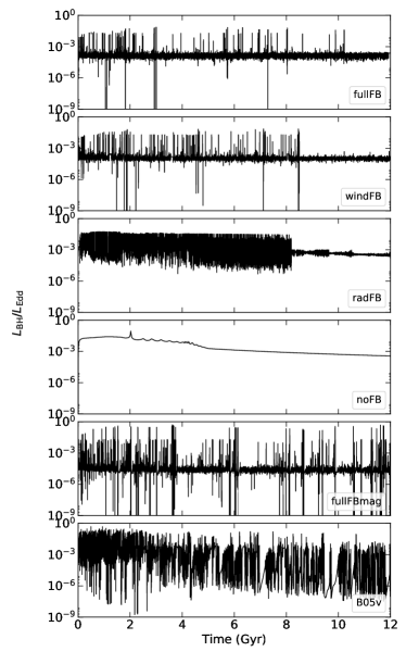
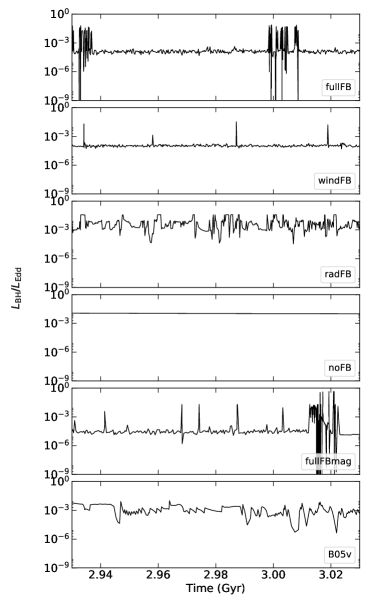
Figure 3.— Light curves of AGN luminosity as a function of time for various models. The left panel is for the whole simulation time while the right panel is for a zoom-in time made between 2.93 and 3.03 Gyr. The data dump time intervals are 2.5 Myr (left panel) and 0.1 Myr (right panel), respectively.
     

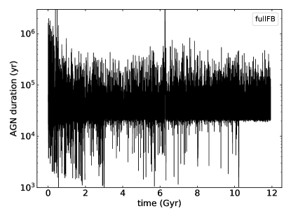
Figure 4.— The duration (or lifetime) of AGN outbursts as a function of evolution time for the fullFB model.

Fig. 3 shows the light curves of the central AGN for each model. For comparison, the “fullFBmag” and “B05v” models are also included. The left panel is for the whole simulation time, while the right one is the zoom-in part made between 2.93 and 3.03 Gyr. Note that for the clarity, when we draw the light curves in the left panel, we choose the data point so that the two adjacent ones have a relatively large time interval; in this case some outbursts are filtered out. But for the right panel of this figure we use the exact simulation data. We see that the light curve of AGN for the noFB model is featureless; once AGN feedback is included in the model, as we explain in the last subsection, the AGN luminosity strongly fluctuates. From the right zoom-in panel for the fullFB model, we can see that the AGN spends most of its time in the low-luminosity phase, with the typical $L_{\rm BH}\sim 10^{-4}L_{\rm Edd}$. We will discuss the AGN duty-cycle in detail in §4.5.

We can see from the figure that the variability amplitudes for the radFB and windFB models are roughly similar, and both of them are similar to the fullFB model. This result indicates that both the mechanical feedback by wind and the radiative feedback by radiation can cause similar amplitude of the AGN variability. However, there is also an important difference. In the time-average sense, especially from the right zoom-in plot, we can see that the AGN luminosity in the radFB model is $\sim 10^{-2}L_{\rm Edd}$, almost two orders of magnitude larger than that in the windFB model, which is $\sim 10^{-4}L_{\rm Edd}$. The main reason for such a big difference is because of the difference of the “typical length scale of feedback”. The length scale for wind (eq. 34) is several orders of magnitude shorter than that for radiation (eq. 33). Therefore, wind can efficiently deposit its momentum and energy into the ISM in a small volume around the black hole, and thus significantly reduce its mass accretion rate. Radiation can only deposit its energy and momentum to the ISM within a much larger scale, and thus is not efficient in reducing the accretion rate. In addition, as shown by Fig. 1, in the cold mode, the momentum flux of wind is larger than that of radiation. This means wind can more effectively push the gas away from the black hole to reduce the accretion rate. We can see that in the fullFB model, the “baseline” AGN luminosity is very similar to that of the windFB model. This indicates that the mass accretion rate of the black hole is controlled by the wind feedback rather than by the radiation. This is what we expect from our analysis presented in §2.4. This also explains that the growth of the black hole mass in the windFB model will be much smaller than that in the radFB model, as we will discuss in §4.3. However, by comparing the right zoom in plots of the fullFB and windFB models, we can see that their light curves are still different, with more outbursts in the fullFB model than in the windFB. This indicates that feedback by radiation and wind may couple together and neither of them can be neglected.

The AGN variability amplitude in both the windFB and radFB models suddenly becomes much smaller after $\sim 8$ Gyr. In addition, different from the epoch before 8 Gyr during which the AGN oscillates between the cold and hot accretion modes, after 8 Gyr the AGN always stays in the low-luminosity hot accretion mode. From Fig. 2, we see that the outbursts of the AGN is because of the accretion of dense gas such as cold clumps. The radiation and especially wind from the AGN is very helpful to the formation of such clumps, since they can perturb the ISM and make its density distribution highly inhomogeneous. Obviously, such kind of perturbation is most strong in the case of cold accretion mode. This argument also explains why the AGN can reach luminosities as low as $\sim 10^{-9}L_{\rm Edd}$ before $\sim 8$ Gyr, which is also because of the strong interaction between AGN and ISM. Because the mass-loss rate from the stellar evolution gradually decays with time and because of the mass lost in the galaxy wind, the gas in the galaxy fueling the black hole becomes fewer with time. This is verified by the gradual decrease of the light curve of the noFB model. Consequently, after $\sim$ 8 Gyr, the AGN can no longer reach the cold accretion mode, thus the perturbation to the ISM becomes much weaker so the clumps are rarely formed. This explains the disappearance of the outbursts after $\sim$ 8 Gyr in both the windFB and radFB models. For the fulFB model, however, we can still find a few outbursts after 8 Gyr. This is because in this model we have both radiative and mechanical feedback thus the perturbation to the ISM is stronger compared to the radFB and windFB models.

Now let us focus on the late epoch of the windFB and radFB models. We can see from the figure that when $t\gtrsim 8$ Gyrs, the AGN luminosity $L_{\rm BH}\lesssim 10^{-3}L_{\rm Edd}$ thus AGN always stays in the hot accretion mode for both models. We can see some variability of AGN in both light curves. The variability amplitude in both cases is small. The main reason is that the radiation and wind are very weak at such a low luminosity. Another reason is that the gas temperature may be high and density low, so that the typical interaction length scale for radiation and wind become very large so the interaction with ISM is not so efficient. The presence of variability in the two models indicates that both wind and radiation have some feedback effects even when they are very weak, at least in terms of modulating the accretion rate. But their respective mechanism may be different. From Fig. 1, we can see that the momentum flux of wind is larger than radiation but the power of radiation is larger than wind. So wind feedback may play its role by momentum interaction while radiation is by energy interaction (radiative heating). The amplitude of variability in the two models are similar, which suggests that the importance of wind and radiation may be similar. It will be an important project to study systematically the importance of feedback by wind and radiation in the hot mode.

Now let us compare the fullFB model with the fullFBmag model. The only difference between these two models is the initial black hole mass. The most significant difference of their light curves is that in the fullFBmag model, the AGN stays in the high-luminosity outburst phase for a longer duration than in the fullFB model. This is explained as follows. Remember that the AGN mass accretion rate is controlled by the wind feedback. When the wind is stronger, the accretion rate is more strongly reduced thus it is harder for the AGN to recover to the high-luminosity outburst phase. When the black hole mass is higher, its accretion rate will be higher thus the bolometric luminosity higher. From eqs. (9) and (12), both the mass flux and velocity of wind are proportional to the bolometric luminosity. So a heavier black hole has stronger wind, thus the duration for the AGN to stay in the high-luminosity outburst phase is shorter.

The fullFBmag and B05v models have the exactly same initial black hole mass, but the AGN physics adopted in the two models is quite different. Such a difference produces very different AGN light curves. From the right zoom in plots, we can see that the typical AGN luminosity of the fullFBmag model is $10^{-4}-10^{-5}L_{\rm Edd}$; while for the B05v model it is more than two orders of magnitude higher, $\sim 10^{-2}L_{\rm Edd}$. The main physical reason for this difference is that the wind adopted in our current paper in both the cold and hot feedback modes are much stronger than that in Gan et al. (2014). A minor reason is that the high value of $T_{\rm C,hot}$ adopted in Gan et al. (2014) makes the temperature of the gas surrounding the black hole as high as $10^{9}~{}{\rm K}$, so $l_{\rm wind}$ becomes much larger, $\sim 5{\rm kpc}$, thus the mechanical feedback becomes much less effective. The less powerful wind and its low feedback efficiency in the B05v model result in a consequence that the AGN variability is dominated by the radiation instead of wind. This is confirmed by the rather similar pattern of light curves between the radFB and B05v models (refer to the right zoom in plots). In contrast to the fullFBmag and fullFB models, the B05v model predicts that the AGN will spend a high fraction of its time staying in the high-luminosity phase. This is not consistent with observations. This indicates the importance of having a correct AGN physics.

Another important consequence of changing the AGN physics is the effect on the typical AGN lifetime (or duration). The AGN lifetime for the fullFB model is shown in Fig. 4. The typical lifetime of the fullFB model is $\sim 10^{5}{\rm yr}$. We define the “on” and “off” of the AGN by comparing its luminosity with the baseline luminosity of the fullFB model, which is $\sim 10^{-4}L_{\rm Edd}$ according to the zoom in plot of fullFB in Fig. 3. As a comparison, the AGN lifetime of the B05v models in Gan et al. (2014) is roughly $\sim 10^{7}{\rm yr}$ (refer to their Fig. 2 and the right panel of Fig. 3). So with the new AGN physics adopted in this paper, the AGN lifetime becomes much shorter. This new value is consistent with the observations (e.g., Martini & Schneider, 2003; Keel et al., 2012; Schawinski et al., 2015). For example, based on the time lag between an AGN switching on and the time the AGN requires to photoionize a large fraction of the host galaxy, Schawinski et al. (2015) estimate that the AGN typically lasts $\sim 10^{5}{\rm yr}$.

4.3. Mass Growth of the Black Hole

$\begin{array}[]{cc}\includegraphics[width=229.81805pt]{mbh_growth.pdf}&\includegraphics[width=195.12767pt]{mbh_growth_mag.pdf}\end{array}$

Figure 5.— Evolution of black hole mass for various models. In the left panel, the upper plot shows the black hole mass growth for the models with an initial black hole mass of $1.8\times 10^{9}\,M_{\odot}$, and the bottom plot shows the black hole mass growth for fullFB, windFB, and fullFBem03 models in detail with linear scale. The right panel is for the two models with an initial black hole mass of $3\times 10^{8}\,M_{\odot}$.

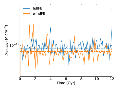
Figure 6.— Time evolution of the gas density at the inner boundary of the simulation for two models. The horizontal dashed lines indicate the time-averaged density.

Fig. 5 shows the evolution of black hole mass for each model. Remember that the initial mass of the black hole is set to be $M_{\rm BH,init}=6\times 10^{-3}\,M_{\star,\rm init}=1.8\times 10^{9}M_{\odot}$ (Kormendy & Ho, 2013). For the noFB model, at the end of evolution the black hole mass reaches as high as over $10^{10}M_{\odot}$, which is obviously too large compared to observations. Since there is no AGN feedback, the gas keeps accreting onto the black hole with little disturbance. In such a situation, mainly only star formation can deplete some gas in the galaxy and reduce the black hole accretion rate which is not very efficient. This is why the black hole can grow to a very large mass.

In the radFB model where only radiative feedback is considered, the black hole mass becomes even slightly larger than the noFB case. This is surprising at the first sight, since one may think the energy input to the gas by AGN radiation should reduce the accretion rate. While this effect must be there, another effect seems to be more important. That is, when the AGN radiation is included, the star formation is suppressed to some degree, mainly due to the radiative heating to the ISM (refer to Fig. 8). Consequently, there will be more gas left and falling onto the inner region of the galaxy to feed the black hole so the accretion rate is higher.

The growth of the black hole in the windFB model is substantially suppressed compared to the noFB model. In fact, the final black hole mass in the windFB model is $2\times 10^{9}M_{\odot}$, only slightly larger than its initial value. This indicates the high efficiency and dominant role of the wind feedback in suppressing the mass accretion rate. The reason has been explained in detail in §4.2. Such a result is in good agreement with Gan et al. (2014) and Ciotti et al. (2017).

However, it is apparently surprising to see from the figure that the black hole mass in the fullFB model is slightly larger than that in the windFB model. One would expect that with the inclusion of radiation, more energy is deposited in the ISM so the accretion rate in the fullFB model should be smaller than windFB model. The reason for the smaller black hole mass in the windFB model is exactly same with what we have just proposed above to explain why the black hole mass is larger in the radFB model compared to noFB model. That is, when radiation is included, star formation becomes weaker thus more gas is left to fuel the black hole. This is confirmed by Fig. 6, which shows the density of the gas at the inner boundary of the simulation for fullFB and windFB models. From this figure we can see that the average gas density in the windFB model is smaller than that in the fullFB model. However, we would caution readers that such a trend of black hole mass change with the feedback models may not be a universal result. In fact, Ciotti et al. (2017) have found both positive and negative change of black hole mass, depending on the mass of galaxies. This is likely because the physics involved is highly non-linear and complicated.

In the model with higher radiative efficiency (fullFBem03), the mass growth of black hole is further suppressed compared with the fullFB model. We think this is not because of the stronger radiative heating due to higher luminosity, but because of the stronger wind in the cold feedback mode, since wind strength is proportional to the luminosity (eqs. (9) & (12)). To check this speculation, we have run another model named “windFBem03” (refer to Table 1). The mass growth of black hole for this model is shown in Figure 5. Both “windFB” and “windFBem03” models include only wind feedback (i.e., no radiation) and the only difference between them is the radiative efficiency. The result shows that the final black hole mass in windFBem03 is smaller than in windFB.

The right plot of Fig. 5 shows the growth of black hole mass for fullFBmag and B05v models. Similar to the fullFB model, the growth of mass in the fullFBmag model is also very small. On the other hand, the growth of black hole mass in the B05v model which has the same initial black hole mass with, but different AGN physics from, the fullFBmag model, is nearly ten times larger. This indicates that the growth of black hole mass is mainly controlled by the AGN physics instead of the black hole mass.

An interesting question is that whether the model can explain the observed correlation between black hole mass and the total mass of stars for elliptical galaxies (e.g., McConnell & Ma, 2013). Ciotti et al. (2017) investigated this problem based on their model and found that the model can explain the observation quite well within the uncertainties. Since the AGN feedback physics adopted in this paper is different from Ciotti et al. (2017), it is necessary to investigate this problem again based on our model. We plan to pursue this problem in our future work.

4.4. Star Formation

Fig. 7 shows the density of newly born stars which was accumulated to the end of our simulation. In general, stars form massively at the cold shells or filaments. The star formation rate is highest at the central region where density is higher, and is quite spherically symmetric due to the low angular momentum of the gas in the galaxy.

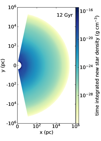
Figure 7.— Time-integrated density of newly born stars at the end of the run for the fullFB model.
    

$\begin{array}[]{ccc}\includegraphics[width=138.76157pt]{newst_c1.pdf}&\includegraphics[width=143.09538pt]{newst_c1_dens.pdf}&\includegraphics[width=138.76157pt]{newst_cum_c1.pdf}\end{array}$

Figure 8.— Effects of AGN feedback on star formation for various models. Left panel: Time-integrated mass of newly born stars at a given radius. Note that the peaks of each curve are simply due to geometry effect; see the text for details. Middle panel: Time-integrated mass of newly born stars at a given radius per unit volume. Right panel: Enclosed mass of the newly born stars within a given radius at the end of the simulation.
    

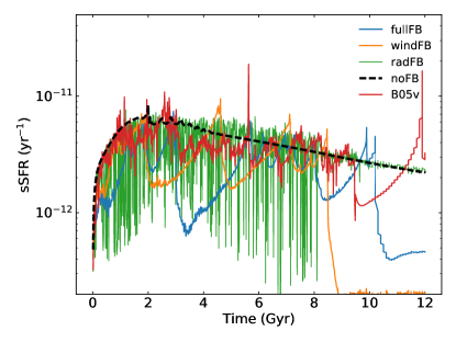
Figure 9.— The specific star formation rate over time for various models.
    

Fig. 8 shows the time- and $\theta$-integrated total mass of newly born star in our simulation. The left panel shows the mass in each radial grid $\Delta r_{i}$ (note that $\Delta r_{i}\propto r$) as a function of radius, while the right panel shows the enclosed mass of the newly born stars within a given radius. In the left panel, the peak of each curve appears at $r\sim 10-30$ kpc. We emphasize that this peak is only an apparent effect and does not mean strong star formation at this radius. Its presence is because the total mass of new stars is integrated within a radial grid $\Delta r_{i}$ while $\Delta r_{i}\propto r$, thus the volume of each grid $\propto r^{3}$. The radius of the peak, i.e., $r\sim 10-30$ kpc, corresponds to the length scale of the galaxy $r_{*}$ (eq. (36)) in the stellar distribution. Beyond this radius the stellar number density sharply decreases thus there are very few gas from stellar wind for the formation of stars. If we normalize the mass of new stars by the volume, the peak will disappear, as shown by the middle panel of Fig.  8.

Now let us see some details of the effects of AGN feedback on star formation. The black dashed line in the left panel denotes model noFB, its peak appears at $\sim 10$ kpc, and there is a rapid increase at the innermost region with the decreasing radius because of the increase of density there. For the radFB model, denoted by the green line, it peaks almost at the same radius with the black dashed line. At the region $r\lesssim$ 600 pc, star formation is significantly suppressed compared with the noFB model. This decrease is perhaps caused by the radiative heating. This radius ($\sim$ 600 pc) is roughly equal to the typical length scale of radiative feedback $l_{\rm rad}$ if $\rho\sim 10^{-23}{\rm g~{}cm^{-3}}$ (eq. (33)). Note that here we adopt a larger density than that shown in Fig. 2; this is because, on the one hand, the density in the radFB model should be higher than that in fullFB since in radFB there is weaker star formation and there is no AGN wind blowing gas out. On the other hand, density varies with time while we should give more weight to the high density since star formation is easier in that case. Beyond 600 pc, the radiation power has been used up thus radiative heating is very weak. In this region, we can see some enhancement of the star formation compared to the noFB mode. This is because radiation force pushes the gas from within $\sim 600$ pc to this region.

For the windFB model, we can see from the left plot that compared to the noFB and also radFB models, star formation is strongly suppressed all the way up to $r\sim 20$ kpc. The peak of the curve also moves outward. The suppressing of star formation is obviously because of the momentum feedback of wind, i.e., winds push the gas away from the central region beyond $\sim 20$ kpc thus the gas density and subsequently star formation is significantly reduced. This is consistent with the suppression of the accretion rate by wind, as we have analyzed in §4.2. At the region $r\gtrsim 20$ kpc, these gas is accumulated there, so star formation is significantly enhanced. Our simulation result that the wind can reach a distance as far as $\sim 20$ kpc is fully consistent with the Gemini Integral Field Unit observations to a sample of radio-quiet quasars (e.g., Liu et al., 2013b)

The solid blue line in the figure denotes the fullFB model. It is quite similar to the windFB model, which indicates that wind feedback is dominant in suppressing the star formation. In the region of $2-20$ kpc, star formation in the fullFB model is slightly stronger than that in the windFB model. The reason is because of the momentum feedback of radiation. Radiation can push the gas away from the region within 2 kpc to this spatial range. This radius (i.e., 2 kpc) is roughly equal to the typical length scale of radiative feedback $l_{\rm rad}$ if $\rho\sim 10^{-24}{\rm g~{}cm^{-3}}$ (eq. (33)). Here $10^{-24}{\rm g~{}cm^{-3}}$ is assumed to be the typical density of ISM. It is lower than that in the fullFB since because both wind and radiation are present in the fullFB model.

Comparing the fullFB model with the noFB model, we can see from the left plot of Fig. 8 that, star formation is suppressed in the inner region of the galaxy, when $r\lesssim 15$ kpc. This is usually called the “negative feedback”. But at the outer region, when $r\gtrsim 15$ kpc, star formation is enhanced. This is the so-called “positive feedback”. We note that the positive feedback effect is consistent with the theoretical result by Liu et al. (2013a) and observations by Cresci et al. (2015), which argued that SF can be enhanced locally at the ahead of the AGN wind, where gas is compressed. Although whether the AGN feedback is positive or negative depends on the location of the galaxy, the overall effect of AGN feedback on star formation in the whole galaxy is negative, as shown by the right plot of Fig. (8). This result is different from Ciotti et al. (2017) where they find the total effect on star formation is positive. The discrepancy must be attributed to the difference of the AGN physics adopted in the two works.

In literature, many observational papers try to study the AGN feedback by investigating the correlation between star formation and AGN activity (see reviews by Harrison 2017 and Xue 2017). From our simulation, we see that the effect of AGN feedback on star formation is very complicated. As we state above, in the time-averaged sense, the effect can be positive or negative, depending on the location of the galaxy. In addition to the spatial complication, we also have temporal complications. AGN activity varies on the timescale of $\tau_{\rm AGN}\lesssim 1$ Myr), which is orders of magnitude shorter than the typical timescale of star formation episodes ($\tau_{\rm SF}\gtrsim 100$ Myrs) (Harrison, 2017). For the whole galaxy, star formation sometimes is enhanced but sometimes suppressed.

To illustrate this point, Fig. 9 shows the specific star formation rate (sSFR) over the galactic evolution, i.e. star formation rate normalized by the stellar mass of the galaxy, which is a quantity widely used in literature. We can see from the figure that the timescale of variability of sSFR is much longer than the variability of AGN, as we explain above. In general, the sSFR in the models with AGN feedback is suppressed compared to noFB model, but occasionally sSFR with AGN feedback can also be enhanced. Another important feature we can see is that the curve of the windFB model is not synchronous with that of fullFB model. While their general patterns are similar, there is an obvious offset between them and the “amplitudes” of the fullFB model are also larger. This indicates that, although from the time-integrated sense wind seems to be much more important than radiation in suppressing star formation, as we see from Fig. 8, radiation definitely also plays a very important role. The wind and radiation likely couple together in affecting star formation. At last, we note that for the windFB and fullFB models, the sSFR sharply decreases at $t\gtrsim 8$ Gyr and $t\gtrsim$ 10 Gyr, respectively. Such sharp decreases correspond to the sudden change of the amplitudes of AGN light curves at the same time for the two models shown in Fig. 3. As we have explained in that section, in that case, there are very few high-density low-temperature clumps in the ISM, and thus star formation becomes very weak.

4.5. AGN Duty Cycle

$\begin{array}[]{cc}\includegraphics[width=216.81pt]{duty_t_c1_below.pdf}&\includegraphics[width=216.81pt]{duty_t_c1_above.pdf}\end{array}$

Figure 10.— Percentage of the total simulation time spent below (left) and above (right) the values of the Eddington ratio of the central AGN for various models. In the left panel, vertical dotted lines indicate the Eddington ratio below which each model spends 80% of the total time. The solid lines are the values for the entire time, and the dashed lines in the right panel are the values for the last 2 Gyrs, which can be compared to observations [square: Ho (2009); circle: Greene & Ho (2007); upward-pointing triangles: Kauffmann & Heckman (2009); downward-pointing triangles: Heckman et al. (2004); star: Steidel et al. (2003).].
    

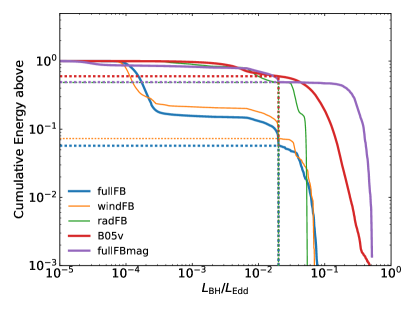
Figure 11.— Percentage of the total energy emitted above the values of the Eddington ratios. The horizontal dotted lines represent the portion of emitted energy above the Eddington ratio of 0.02.
    

Fig. 10 shows the percentage of the total simulation time spent below (left panel) and above (right panel) a given Eddington ratio. In the left panel, the vertical dotted lines indicate the Eddington ratio below which the AGN spends 80% of its time. Comparing various models, we can see that from radFB to fullFB (windFB is similar), with the increase of AGN feedback “strength”, this Eddington ratio becomes smaller. Among all models, the ratio is the smallest for the fullFBmag model. This is consistent with that shown in the right panel of Fig. 3 in which the fullFBmag model has the lowest typical Eddington ratio. For the fullFB model, the AGN spends over 80% of its evolution time with Eddington ratios below $2\times 10^{-4}$ and it spends most of its time in the hot accretion (feedback) mode. This results suggests that potential importance of feedback effects by low-luminosity AGNs.

In the right panel of Fig. 10, we compare the simulation results with observations. The solid and dashed lines represent the time spent above the given Eddington ratios for entire evolution time and for the last 2 Gyrs, respectively. The observational data points are compiled from low-redshift sources, which are suitable to be compared with the dashed lines. For the blue dashed line, which denotes the fullFB model in the late epoch, the AGN spends very little of its time being in the luminosity of $L_{\rm BH}/L_{\rm Edd}\gtrsim 1\%$. This can also be roughly seen from the left panel of Fig. 3. This result is consistent with observations (e.g., Steidel et al., 2003; Heckman et al., 2004; Greene & Ho, 2007; Ho, 2009; Kauffmann & Heckman, 2009).

It is believed that AGNs spend most of their time in the low-luminosity AGN phase, but emit most of their energy during their high-luminosity AGN phase (Soltan, 1982; Yu & Tremaine, 2002; Kollmeier et al., 2006). To examine this issue with our simulations, Fig. 11 shows the percentage of the total energy emitted above the values of the Eddington ratios for various models. Specifically, the horizontal dotted lines mark the fraction of emitted energy with the Eddington ratio above 0.02. For the fullFB models, the AGN emits $6\%$ of the entire energy at the Eddington ratio above 0.02. The percentage for the fullFB model is much lower than what observations seem to suggest. There are two main reasons for this discrepancy. One is that our simulations begin from 2 Gyr. Before 2 Gyr, the activity of AGN should be much stronger. Another reason is that the present paper only focuses on an isolated galaxy. The percentage of energy emitted is expected to increase significantly if we also include the cosmic accretion of cold gas from outside of the galaxy.

We note that for the fullFBmag model, AGN emits $50\%$ of the entire energy at the Eddington ratio above 0.02. This is much closer to the observation compared to model fullFB. There are two reasons for such a discrepancy between “fullFB” and “fullFBmag”. One is that when the black hole mass is smaller as in fullFBmag, the AGN becomes weaker thus it becomes more difficult to push the gas surrounding the black hole away so the mass accretion rate is in general larger. Another reason is that the critical luminosity (eq. (1)) separating the hot and cold modes is proportional to the black hole mass. When the black hole mass is smaller, it is easier for the AGN to switch from the hot to the cold accretion modes. These two reasons make the AGN with a smaller black hole mass spend more time above a given Eddington ratio, as shown by the right plot of Fig. 10, and subsequently emit more energy above a given Eddington ratio.

The two models fullFBmag and B05v have the same black hole mass, we can see they are similar in Fig. 11. However, these two models are quite different in Fig. 10. The fullFBmag model spends much fewer time above a given Eddington ratio compared to model B05v. Such a discrepancy is caused by the difference of AGN physics. Specifically, the wind in fullFBmag model is much stronger than in B05v thus the black hole accretion rate in fullFBmag is generally much smaller.

4.6. X-ray Properties of the Gas

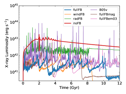
Figure 12.— The evolution of the X-ray luminosity of the galaxy in the 0.3-8 keV band for various models.
    

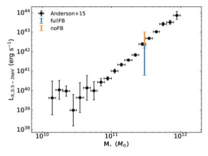
Figure 13.— Comparison of the X-ray luminosity of the hot gas in the 0.5-2 keV band between our simulations and the observations by Anderson et al. (2015). The black dots with error bars are the observational data, while the orange and blue segments denote the simulation results of the noFB and fullFB models.

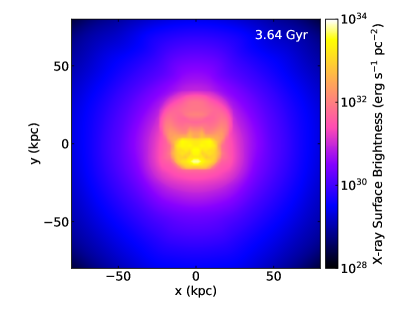
Figure 14.— X-ray surface brightness in the 0.3-8 keV band for the fullFB model.

The X-ray luminosity of the galactic hot gas content, which is mainly produced by bremsstrahlung, is observable for active galaxies (Brandt & Alexander, 2015, and references therein). It is calculated over the energy range of 0.3-8 keV (the Chandra sensitive band), which is

$$L_{\rm X}=4\,\pi\int^{\infty}_{0}\,\varepsilon\left(r\right)\,r^{2}\,dr,$$ (51)

where the emissivity is given by $\varepsilon(r)=n_{e}(r)n_{\rm H}(r)\Lambda\left[T(r)\right]$, with $n_{e}$ and $n_{\rm H}$ are the number densities of electron and hydrogen, and $\Lambda\left(T\right)$ is the cooling function. We fix the metallicity to the solar abundance. The cooling function is calculated by the spectral fitting package XSPEC (spectral model APEC) with the assumption of the collisional ionization equilibrium (Smith et al., 2001), and the volume integrals are performed over the whole computational mesh.

Fig. 12 shows the evolution of the X-ray luminosity, $L_{\rm X}$, for various models. For the models with AGN feedback, $L_{\rm X}$ oscillates in phase with the nuclear luminosity, which is consistent with Pellegrini et al. (2012): radiative and mechanical feedback change the density and temperature of the gas in the galactic center, where most of $L_{\rm X}$ is emitted. On the contrary, in the noFB model, the light curve of $L_{\rm X}$ is quite smooth and monotonously decreases as a consequence of gas depletion due to star formation. The average value of the X-ray luminosity for various models follows this order: noFB $>$ radFB $>$ fullFB (windFB) $>$ fullFBmag. This sequence is consistent with the light curves shown for various models in Fig. 3. It is interesting to note that the pattern or the shape of the X-ray luminosity for the windFB and fullFB models is very similar to the sSFR shown in Fig. 9. This is reasonable since both the sSFR and the X-ray luminosity depend on the local properties of gas on large scales.

Anderson et al. (2015) have stacked X-ray emission from ROSAT All-Sky Survey in the X-ray band range of 0.5-2 keV, and showed the power-law relationship between the X-ray luminosity and the stellar mass of the central galaxy. To compare with this observation, we have calculated the X-ray luminosity of the hot gas in the 0.5-2 keV band. The result is shown in Fig. 13. Since the X-ray luminosity is variable, we show in the figure the full range of luminosity. We can see from the figure that the noFB model predicts a higher luminosity than the fullFB model, as we expect, and both of their predictions are marginally consistent with the observations. However, considering that our current work focuses only on isolated galaxy and has not taken into account the gas supply from outside of the galaxy while the X-ray luminosity values taken from Anderson et al. (2015) are for central galaxies, the fullFB model is more promising to be consistent with observations while the noFB model will likely over-predict the luminosity once we more properly consider the additional external gas supply. As comparison, Eisenreich et al. (2017) recently have also compared their numerical simulation result with the observations of Anderson et al. (2015). They find that the simulated value is a factor of few too high. They speculated that the reason may be because of their initial condition of simulation. But another possible reason is the AGN physics they adopt.

In order to calculate X-ray surface brightness, we first generate three-dimensional data based on our two-dimensional numerical simulation data by assuming axisymmetry and then integrating the emissivity along the line-of-sight. Fig. 14 shows the X-ray surface brightness for the model fullFB during an AGN outburst. We can see from the figure that an X-ray cavity forms when AGN feedback expels and heats the gas in the galactic center, and such a cavity looks very similar to those observed (e.g., Fabian 2012 and references therein). We have also checked the windFB and radFB models and found that the cavity is formed almost fully by the interaction between wind and ISM, not because of radiative heating to the ISM. We note that in literature people usually think that the observed X-ray cavity is formed by the interaction between jet and ISM (Guo, 2016; Guo et al., 2018). The reason may be because jets are very common but winds are harder to be detected. However, we would like to emphasize that non-detection does not mean non-existence. We now know that jet is an indispensable ingredient of hot accretion flows (Yuan & Narayan, 2014); while in hot accretion flows we now have compelling evidences for the existence of wind, from both theoretical (Yuan et al., 2012; Narayan et al., 2012; Yuan & Narayan, 2014; Yuan et al., 2015) and observational (see references in §2.3.2) aspects. In other words, whenever we observe jet, wind must also exist. So the formation of X-ray cavity shown in Fig. 14 suggests that it is worthwhile to investigate the possibility that the cavities usually observed are formed by wind. In fact, winds launched from hot accretion flow have been used to successfully explain the formation of the Fermi bubbles observed in the Galaxy (Mou et al., 2014, 2015). Compared with other models of the Fermi bubbles (e.g., Guo & Mathews, 2012), this “wind” model has the following advantages: 1) the main parameters of the model such as mass flux and velocity of wind are well constrained by the small-scale MHD numerical simulation (Yuan et al., 2015), thus has much less freedom; 2) the model can successfully explain some observations of the Fermi bubbles that are hard to be explained by other models (see Mou et al. 2015 for details).

5. Summary and Conclusions

In this paper, by performing two-dimensional high-resolution hydrodynamical numerical simulations, we have investigated the effects of AGN feedback in the evolution of its host galaxy. The galaxy is an isolated elliptical galaxy and we assume in this work that the specific angular momentum of the gas is low. Physical processes like star formation, Type Ia and Type II supernovae are taken into account. The inner boundary of the simulation is chosen so that the Bondi radius is resolved, which is crucial for the precise determination of the mass accretion rate of the AGN. According to the theory of black hole accretion, black hole accretion has two intrinsically different modes, cold and hot ones. They have quite different radiation and wind outputs and thus naturally correspond to two different feedback modes. They have been carefully discriminated and taken into account in the present work. We consider the feedback effects by both radiation and wind in each mode. The two feedback modes have quite diverse names in literature, e.g., the quasar (or radiative) and radio (or kinetic or maintenance) mode. Our present work indicates that these names are not only diverse, but sometimes also misleading. For example, in terms of regulating the accretion rate of the black hole and star formation in the galaxy, feedback by wind is always much more important that radiation. So we suggest to simply follow the names of black hole accretion mode and call them “cold feedback mode” and “hot feedback mode”.

The most important distinctive feature of the present work is that we adopt the most updated AGN physics. This is especially the case for the radiation and wind from hot accretion flows for which many progresses have been made in recent years but have not been taken into account in most AGN feedback works (see a recent review by Yuan & Narayan, 2014). It also includes more precise descriptions of wind in the cold mode which are obtained from recent new observations. These most updated AGN physics are summarized in the present paper. For the feedback effects, we have investigated the light curve of the AGN, the black hole growth, star formation, the AGN duty-cycle, and the surface brightness of the galaxy. We have compared these results with previous works which have very similar model framework with our work but have different AGN physics. Significantly different results have been found in almost every aspect mentioned above. This indicates the crucial importance of having correct AGN physics. The main results obtained in this paper are summarized below.

• We have compared the energy and momentum fluxes of wind and radiation in the two feedback modes (Fig. 1). Roughly speaking, in both modes, the power of radiation is larger than wind while the momentum flux is on the opposite. However, the magnitude of energy or momentum fluxes is not the only factor to determine which component, radiation or wind, is more important in the feedback. This is because the cross section of photon-particle interaction is orders of magnitude smaller than that of particle-particle interaction. For typical parameters of our problem, we find that wind can deposit its momentum within a very small “typical length scale of wind feedback”, $l_{\rm wind}\sim 0.5$ pc (Eq. 34); while the “typical length scale of radiation feedback” is much larger, $l_{\rm rad}\sim 10$ kpc (Eq. 33). Consequently, in our model the accretion rate and the mass growth of black hole are mainly suppressed by wind rather than radiation (compare the zoom in plots of windFB, fullFB, and radFB in Fig. 3; and windFB, fullFB, and radFB in Fig. 5). Such a result is in good agreement with Gan et al. (2014) and Ciotti et al. (2017). But we note there are two caveats here. One is that in the present paper we consider an isolated galaxy without external gas supply. Another one is that we do not consider dust. If we consider these two factors, the radiative feedback should become relatively more important.

• One characteristic consequence when the AGN feedback is included in the galaxy evolution model is that the AGN activity becomes strongly variable (Fig. 3). The reason is because of the interaction between wind & radiation and ISM (§4.1). Both radiation or wind can cause the variability of AGN but their mechanisms are different. Wind is by momentum interaction while radiation is by radiative heating. Because the typical length scale of wind feedback is much shorter than that of radiation, the accretion rate of AGN is reduced to a much lower time-averaged value in the windFB model than in the radFB model (right panel of Fig. 3). But radiation also plays an important role, maybe by coupling with the wind feedback. Comparison with previous works which have different AGN physics indicates that stronger wind in the AGN physics results in a time-averaged weaker AGN (compare the zoom in plot of fullFB and B05v in Fig. 3).

• The typical lifetime of the AGN obtained by our simulation is $\sim 10^{5}$ yr, fully consistent with the most recent observations (Fig. 4). As a comparison, previous works which have different AGN physics, such as Gan et al. (2014), obtain a much longer AGN lifetime.

• Both radiation and wind can suppress the star formation in the galaxy. In our model, radiation can affect the region of “unity optical depth”, $\sim 1$ kpc, while wind can affect a much larger region, $\lesssim 20$ kpc (the left plot of Fig. 8). Not only the affected scale is different, the wind can also suppress the star formation much more strongly than radiation (the left plot of Fig. 8). Beyond $20~{}{\rm kpc}$, star formation is enhanced, because of the accumulation of gas pushed out by wind. Overall, we find that the time-integrated total effect of AGN feedback on star formation is negative (right panel of Fig. 8). But we would like to emphasize that whether the feedback can suppress or enhance star formation not only depends on the spatial location but also on time. The spatially-integrated specific star formation rate (sSFR) as a function of time shows two important features. One is that depending on the evolution time, sSFR can be enhanced or suppressed compared to the model without AGN feedback. The second one is that radiation also plays a very important role in affecting star formation (compare windFB and fullFB models in Fig. 9).

• When all the feedback mechanisms have been considered, we find that the AGNs spend over 80% of their time with Eddington ratio below $2\times 10^{-4}$, i.e., in the very low-luminosity regime (the left panel of Fig. 10). This suggests the importance of considering the hot mode feedback in the galaxy evolution. We have also compared the simulated percentage of the last 2 Gyrs spent above a given Eddington ratio with observations. We find that the AGN has very little of its time being in the range of $L_{\rm BH}/L_{\rm Edd}\gtrsim 1\%$, consistent with observations (right panel of Fig. 10). We have also calculated the percentage of the total energy emitted above a given Eddington ratio. For our fullFB model, it is only $6$% at Eddington ratio above 0.02. This value is not consistent with what we believe. An important reason is that we assume an isolated galaxy and have not taken into account the external gas supply in our simulations.

• We have calculated the X-ray luminosity of the hot gas in the galaxy in the 0.5-2 keV band and compared the result with observations. Both models with and without AGN feedback are consistent with observations given their large error bars (Fig. 13). But once we include external gas supply in the future, the noFB model may overpredict the observed value.

• The X-ray surface brightness for the model fullFB during an AGN outburst is calculated (Fig. 14). An X-ray cavity surrounding the AGN is evident, which is formed by the interaction between wind and ISM. It looks very similar to the X-ray cavities observed in galaxy clusters (e.g., Fabian, 2012). Usually we think these X-ray cavities are formed by jets. So this result suggests us to consider the possibility that they are formed by wind.

References

- Anderson et al. (2015) Anderson, M. E., Gaspari, M., White, S. D. M., Wang, W., & Dai, X. 2015, MNRAS, 449, 3806
- Bieri et al. (2017) Bieri, R., Dubois, Y., Rosdahl, J., et al. 2017, MNRAS, 464, 1854
- Blaes (2014) Blaes, O. 2014, Space Sci. Rev., 183, 21
- Blustin et al. (2007) Blustin, A. J., Kriss, G. A., Holczer, T., et al. 2007, A&A, 466, 107
- Bondi (1952) Bondi, H. 1952, MNRAS, 112, 195
- Booth & Schaye (2009) Booth, C. M., & Schaye, J. 2009, MNRAS, 398, 53
- Brandt & Alexander (2015) Brandt, W. N., & Alexander, D. M. 2015, A&A Rev., 23, 1
- Bu & Yuan (2014) Bu, D.-F., & Yuan, F. 2014, MNRAS, 442, 917
- Bu et al. (2016) Bu, D.-F., Yuan, F., Gan, Z.-M., & Yang, X.-H. 2016, ApJ, 823, 90
- Cheung et al. (2016) Cheung, E., Bundy, K., Cappellari, M., et al. 2016, Nature, 533, 504
- Choi et al. (2012) Choi, E., Ostriker, J. P., Naab, T., & Johansson, P. H. 2012, ApJ, 754, 125
- Choi et al. (2015) Choi, E., Ostriker, J. P., Naab, T., Oser, L., & Moster, B. P. 2015, MNRAS, 449, 4105
- Ciotti et al. (2009) Ciotti, L., Morganti, L., & de Zeeuw, P. T. 2009, MNRAS, 393, 491
- Ciotti & Ostriker (2007) Ciotti, L., & Ostriker, J. P. 2007, ApJ, 665, 1038
- Ciotti & Ostriker (2012) Ciotti, L., & Ostriker, J. P. 2012, in Astrophysics and Space Science Library, Vol. 378, Astrophysics and Space Science Library, ed. D.-W. Kim & S. Pellegrini, 83
- Ciotti et al. (2010) Ciotti, L., Ostriker, J. P., & Proga, D. 2010, ApJ, 717, 708
- Ciotti et al. (2017) Ciotti, L., Pellegrini, S., Negri, A., & Ostriker, J. P. 2017, ApJ, 835, 15
- Costa et al. (2017) Costa, T., Rosdahl, J., Sijacki, D., & Haehnelt, M. G. 2017, ArXiv e-prints, arXiv:1709.08638
- Crenshaw & Kraemer (2012) Crenshaw, D. M., & Kraemer, S. B. 2012, ApJ, 753, 75
- Crenshaw et al. (2003) Crenshaw, D. M., Kraemer, S. B., & George, I. M. 2003, ARA&A, 41, 117
- Cresci et al. (2015) Cresci, G., Mainieri, V., Brusa, M., et al. 2015, ApJ, 799, 82
- Czoske et al. (2008) Czoske, O., Barnabè, M., Koopmans, L. V. E., Treu, T., & Bolton, A. S. 2008, MNRAS, 384, 987
- Debuhr et al. (2011) Debuhr, J., Quataert, E., & Ma, C.-P. 2011, MNRAS, 412, 1341
- Di Matteo et al. (2005) Di Matteo, T., Springel, V., & Hernquist, L. 2005, Nature, 433, 604
- Díaz Trigo & Boirin (2016) Díaz Trigo, M., & Boirin, L. 2016, Astronomische Nachrichten, 337, 368
- Djorgovski & Davis (1987) Djorgovski, S., & Davis, M. 1987, ApJ, 313, 59
- Dye et al. (2008) Dye, S., Evans, N. W., Belokurov, V., Warren, S. J., & Hewett, P. 2008, MNRAS, 388, 384
- Eisenreich et al. (2017) Eisenreich, M., Naab, T., Choi, E., Ostriker, J. P., & Emsellem, E. 2017, MNRAS, 468, 751
- Faber & Jackson (1976) Faber, S. M., & Jackson, R. E. 1976, ApJ, 204, 668
- Fabian (2012) Fabian, A. C. 2012, ARA&A, 50, 455
- Fender (2003) Fender, R. P. 2003, MNRAS, 340, 1353
- Frank et al. (2002) Frank, J., King, A., & Raine, D. J. 2002, Accretion Power in Astrophysics: Third Edition, 398
- Gaibler et al. (2012) Gaibler, V., Khochfar, S., Krause, M., & Silk, J. 2012, MNRAS, 425, 438
- Gan et al. (2014) Gan, Z., Yuan, F., Ostriker, J. P., Ciotti, L., & Novak, G. S. 2014, ApJ, 789, 150
- Gaspari et al. (2013) Gaspari, M., Ruszkowski, M., & Oh, S. P. 2013, MNRAS, 432, 3401
- Gaspari & Sa̧dowski (2017) Gaspari, M., & Sa̧dowski, A. 2017, ApJ, 837, 149
- Gaspari et al. (2018) Gaspari, M., McDonald, M., Hamer, S. L., et al. 2018, ApJ, 854, 167
- Gofford et al. (2015) Gofford, J., Reeves, J. N., McLaughlin, D. E., et al. 2015, MNRAS, 451, 4169
- Greene & Ho (2007) Greene, J. E., & Ho, L. C. 2007, ApJ, 667, 131
- Gu & Lu (2000) Gu, W.-M., & Lu, J.-F. 2000, ApJ, 540, L33
- Gültekin et al. (2009) Gültekin, K., Richstone, D. O., Gebhardt, K., et al. 2009, ApJ, 698, 198
- Guo (2016) Guo, F. 2016, ApJ, 826, 17
- Guo et al. (2018) Guo, F., Duan, X., & Yuan, Y.-F. 2018, MNRAS, 473, 1332
- Guo & Mathews (2012) Guo, F., & Mathews, W. G. 2012, ApJ, 756, 181
- Hamann et al. (2008) Hamann, F., Kaplan, K. F., Rodríguez Hidalgo, P., Prochaska, J. X., & Herbert-Fort, S. 2008, MNRAS, 391, L39
- Häring & Rix (2004) Häring, N., & Rix, H.-W. 2004, ApJ, 604, L89
- Harrison (2017) Harrison, C. M. 2017, Nature Astronomy, 1, 0165
- Hayes et al. (2006) Hayes, J. C., Norman, M. L., Fiedler, R. A., et al. 2006, ApJS, 165, 188
- Heckman et al. (2004) Heckman, T. M., Kauffmann, G., Brinchmann, J., et al. 2004, ApJ, 613, 109
- Hirschmann et al. (2014) Hirschmann, M., Dolag, K., Saro, A., et al. 2014, MNRAS, 442, 2304
- Ho (1999) Ho, L. C. 1999, ApJ, 516, 672
- Ho (2008) —. 2008, ARA&A, 46, 475
- Ho (2009) —. 2009, ApJ, 699, 626
- Homan et al. (2016) Homan, J., Neilsen, J., Allen, J. L., et al. 2016, ApJ, 830, L5
- Hopkins & Quataert (2011) Hopkins, P. F., & Quataert, E. 2011, MNRAS, 415, 1027
- Ishibashi & Fabian (2015) Ishibashi, W., & Fabian, A. C. 2015, MNRAS, 451, 93
- Jaffe (1983) Jaffe, W. 1983, MNRAS, 202, 995
- Kato et al. (2008) Kato, S., Fukue, J., & Mineshige, S. 2008, Black-Hole Accretion Disks — Towards a New Paradigm —
- Kauffmann & Heckman (2009) Kauffmann, G., & Heckman, T. M. 2009, MNRAS, 397, 135
- Keel et al. (2012) Keel, W. C., Chojnowski, S. D., Bennert, V. N., et al. 2012, MNRAS, 420, 878
- King & Pounds (2015) King, A., & Pounds, K. 2015, ARA&A, 53, 115
- Kollmeier et al. (2006) Kollmeier, J. A., Onken, C. A., Kochanek, C. S., et al. 2006, ApJ, 648, 128
- Kormendy & Ho (2013) Kormendy, J., & Ho, L. C. 2013, ARA&A, 51, 511
- Le Brun et al. (2014) Le Brun, A. M. C., McCarthy, I. G., Schaye, J., & Ponman, T. J. 2014, MNRAS, 441, 1270
- Li et al. (2013) Li, J., Ostriker, J., & Sunyaev, R. 2013, ApJ, 767, 105
- Li et al. (2018) Li, Y.-P., Yuan, F., Mo, H., et al. 2018, ArXiv e-prints, arXiv:1803.01444
- Liu et al. (1999) Liu, B. F., Yuan, W., Meyer, F., Meyer-Hofmeister, E., & Xie, G. Z. 1999, ApJ, 527, L17
- Liu et al. (2013a) Liu, C., Gan, Z.-M., & Xie, F.-G. 2013a, Research in Astronomy and Astrophysics, 13, 899
- Liu et al. (2015) Liu, G., Arav, N., & Rupke, D. S. N. 2015, ApJS, 221, 9
- Liu et al. (2013b) Liu, G., Zakamska, N. L., Greene, J. E., Nesvadba, N. P. H., & Liu, X. 2013b, MNRAS, 436, 2576
- Magorrian et al. (1998) Magorrian, J., Tremaine, S., Richstone, D., et al. 1998, AJ, 115, 2285
- Manmoto & Kato (2000) Manmoto, T., & Kato, S. 2000, ApJ, 538, 295
- Martini & Schneider (2003) Martini, P., & Schneider, D. P. 2003, ApJ, 597, L109
- McCarthy et al. (2017) McCarthy, I. G., Schaye, J., Bird, S., & Le Brun, A. M. C. 2017, MNRAS, 465, 2936
- McCarthy et al. (2010) McCarthy, I. G., Schaye, J., Ponman, T. J., et al. 2010, MNRAS, 406, 822