Nonlinear optical responses of crystalline systems:
Results from a velocity gauge analysis

Abstract

In this work, the difficulties inherent to perturbative calculations in the velocity gauge are addressed. In particular, it is shown how calculations of nonlinear optical responses in the independent particle approximation can be done to any order and for any finite band model. The procedure and advantages of the velocity gauge in such calculations are described. The addition of a phenomenological relaxation parameter is also discussed. As an illustration, the nonlinear optical response of monolayer graphene is numerically calculated using the velocity gauge.

I INTRODUCTION

A common approach to understanding nonlinear optical effects in atomic and condensed matter systems comes from a perturbation theory where the electric current is expanded in powers of an external applied electric field shen1984principles , assumed to be sufficiently weak for the expansion to be physically meaningful. In this framework, one attempts to calculate nonlinear optical response functions, usually second or third order susceptibilities, the different frequency components of which describe a variety of physical phenomena like the Kerr effect, harmonic generation, electro-optic effect, etc.

The theory was first developed for atomic systems and, in the early nineties sipe1993nonlinear ; aversa1995nonlinear , extended to crystalline systems, characterized by electronic bands and the corresponding Bloch functions. The simpler calculations follow two essential assumptions which will be adopted throughout this work: the independent particle approximation, where explicit electron-electron interactions are disregarded (except possibly in the determination of the electron bands, as in Density Functional Theory), and the electric dipole approximation, where the response functions are taken to be local in space, a consequence of the long wavelength limit of the applied electric field.

Even in this simple approach, however, difficulties were found regarding different ways to describe the perturbation. We can write the complete Hamiltonian of the crystal under the influence of the external field in two ways, either in the length gauge,

$$H(t)=H_{0}(\textbf{r},\textbf{p})-q\,\textbf{r}\cdot\textbf{E}(t),$$ (1)

or in the velocity gauge or minimal coupling Hamiltonian,

$$H(t)=H_{0}(\textbf{r},\textbf{p}-q\textbf{A}(t)),$$ (2)

where $H_{0}$ is the unperturbed crystal Hamiltonian, $q=-e$ is the charge of the electron and $\textbf{A}(t)$ the vector potential, chosen so that $\textbf{E}(t)=-\partial_{t}\textbf{A}(t)$. These two descriptions can easily be shown to be equivalent and related by a time-dependent unitary transformation ventura2017gauge .

The first attempts at computing nonlinear optical responses in crystals made use of the minimal coupling method genkin1968contribution ; sipe1993nonlinear , since it has the advantage of retaining the translation symmetry of the Hamiltonian, only coupling states with the same Bloch vector k. However, it presented some serious difficulties as it seemed that response functions computed in the velocity gauge diverged in the limit of low frequencies, even for the case of zero temperature insulators, where such divergences should clearly be absent. A more detailed analysis of the linear response showed that these were only apparent divergences that could be removed by careful manipulations and sum rules sipe1993nonlinear . As presented, these procedures were cumbersome and not easily generalizable to higher order response functions.

This led to a preference for the length gauge in nonlinear optical response calculations aversa1995nonlinear ; hughes1996calculation ; sipe2000second ; al2014high ; hipolito2016nonlinear . This gauge presents its own difficulties, the most notorious one being that the matrix elements of the position operator in the Bloch basis are ill-defined until the thermodynamic limit is taken and, even then, they can be defined only as a distribution. Inspired by Blount’s work blount1962formalisms , Aversa et al. aversa1995nonlinear pointed out that the position operator will appear in the calculations only inside commutators whose matrix elements are well defined and successfully developed the theory in the length gauge. This formalism has since been applied to various systems cheng2014dc ; cheng2015third ; hipolito2016nonlinear ; hughes1996calculation ; nastos2005scissors ; al2014high .

More recently, and still within the length gauge approach, simple expressions for the nonlinear conductivity to arbitrary order in the electric field were derived by the present authors, making use of the covariant derivative notation ventura2017gauge . These expressions are useful for inspection and reduced the calculation procedure to a fairly straightforward expansion of commutators. Although the idea of a “generalized derivative” was already around in the literature aversa1995nonlinear , it involved separating the intra and inter-band components of the position operator and response functions. The emphasis on these distinctions, originally motivated by the intent of applying the equations to the special case of clean, cold semiconductors and to make analogies with atomic and free electron systems, made the calculations less transparent, in our view.

In this same work ventura2017gauge , similar and equivalent expressions were derived using the velocity gauge, for the Hamiltonian

$$H_{0}(\mathbf{r},\mathbf{p})=\frac{\mathbf{p}^{2}}{2m}+V_{L}(\mathbf{r}),$$ (3)

where the second term is the periodic lattice potential. It was shown that, in the form derived from the velocity gauge, the expressions for the nonlinear optical coefficients lose their validity if only a finite number of bands around the Fermi level are taken into account. This difficulty was recognized early on aversa1994third ; aversa1995nonlinear , and, together with the apparent infrared divergences, led to the velocity gauge being less adopted. The reasons for the failure of these expressions under a truncation in band space were also understood rzkazewski2004equivalence ; aversa1995nonlinear and recently subjected to a more quantitative analysis taghizadeh2017linear . One of the arguments aversa1995nonlinear consisted in noting that the sum rules that connected the expressions in the two gauges seem to rely on commutator identities such as

$$\left[r^{\alpha},v^{\beta}\right]=\frac{i\hbar}{m}\,\delta^{\alpha\beta}$$ (4)

($\mathbf{r}$ and $\mathbf{v}$, position and velocity operators), which require an infinite number of bands to hold. This led to a common misconception that the velocity gauge could only be properly implemented if an infinite number of bands is taken into account aversa1994third ; aversa1995nonlinear ; virk2007semiconductor ; cheng2014third ; al2014high ; taghizadeh2017linear . In fact, sum rules of greater generality have been constructed which remain true even under truncation of the bands ventura2017gauge . Nonetheless, various authors have indicated that the velocity gauge, if employed, would lead to different, unphysical, predictions virk2007semiconductor ; taghizadeh2017linear .

The fundamental difference between the two gauges that seems not to have been properly appreciated concerns the form of the perturbation. In the velocity gauge, the form of the perturbation depends explicitly on $H_{0}$, unlike in the case of the length gauge. Expressions for the nonlinear coefficients derived from the Hamiltonian in Eq. 3, cannot be truncated to a finite set of bands. A truncation of $H_{0}$ implies a different form of the perturbation, and leads to different expressions for the nonlinear conductivities in the velocity gauge, but not in the length gauge.

In order to build the theory in its most general form, we will make no assumptions on the form of $H_{0}$, other than it has the periodicity of some Bravais lattice, so that Bloch’s theorem applies and there is a well defined First Brillouin Zone (FBZ). The derived forms for the nonlinear conductivities will be completely equivalent to the ones obtained from the length gauge and can be applied to any finite band model; no commutator identities of the kind of Eq. 4 are assumed.

In the next section, the equivalence of the two gauges is revisited, starting from an Hamiltonian with a finite set of bands, and some formal concepts behind the velocity gauge formulation are reviewed. In section III, the equation of motion for the reduced density matrix in the velocity gauge is introduced in a form more general than previously presented. Recursively solving the equation of motion leads to the nonlinear conductivities. The advantages and subtleties of using this gauge are discussed in Section IV, where it is argued that the velocity gauge should prove more efficient for numerical computations. In Section V, the introduction of a phenomenological relaxation parameter is addressed, and proves to be less trivial than expected. As an example, in Section VI the formalism is applied to third harmonic generation in graphene, in a full Brillouin zone calculation, and a comparison is made with already existing results in the literature. Section VII contains some closing remarks.

II DENSITY MATRIX FORMALISM

In very general terms, which do not exclude finite band models, the single particle unperturbed Hamiltonian $H_{0}$ can be written as

$$H_{0}=\sum_{s}\int\!\frac{d^{d}\textbf{k}}{(2\pi)^{d}}\left|\psi_{\textbf{k}s}\right\rangle\left[H_{0}\right]_{\mathbf{k}ss}\left\langle\psi_{\textbf{k}s}\right|,$$ (5)

where $\left|\psi_{\textbf{k}s}\right\rangle$ are the Bloch band states and $\left[H_{0}\right]_{\mathbf{k}ss^{\prime}}\equiv\epsilon_{\mathbf{k}s}\delta_{ss^{\prime}}$, with $\epsilon_{\mathbf{k}s}$ the band energies.

To represent the scalar potential, $-q\,\mathbf{E}\cdot\mathbf{r}$, in the Bloch basis, we require from the start the infinite volume limit. We define the normalization of the Bloch wave functions as

$$\langle\psi_{\mathbf{k}^{\prime}s^{\prime}}|\psi_{\mathbf{k}s}\rangle=\left(2\pi\right)^{d}\delta_{ss^{\prime}}\delta\left(\mathbf{k}-\mathbf{k}^{\prime}\right).$$ (6)

where $d$ is the dimensionality of the system. Using Blount’s results for the matrix elements of the position operator blount1962formalisms ,

$$\left\langle\psi_{\mathbf{k}s}\right|\mathbf{r}\left|\psi_{\mathbf{k^{\prime}s^{\prime}}}\right\rangle =(2\pi)^{d}\left[\delta_{ss^{\prime}}(-i)\nabla_{\mathbf{k}^{\prime}}\delta(\mathbf{k}^{\prime}-\mathbf{k})\right.$$

$$+\left.\delta(\mathbf{k}-\mathbf{k}^{\prime})\,\bm{\xi}_{\mathbf{k}ss^{\prime}}\right],$$ (7)

where $\xi_{\textbf{k}ss^{\prime}}$ is the Berry connection berry1984quantal ; xiao2010berry , one obtains for the single particle perturbed Hamiltonian in the length gauge ventura2017gauge (see Appendix B)

$$H^{E}=\int\frac{d^{d}\mathbf{k}}{(2\pi)^{d}}\sum_{s,s^{\prime}}\left|\psi_{\mathbf{k}s}\right\rangle\left[\delta_{ss^{\prime}}\epsilon_{\mathbf{k}s}-iq\mathbf{E}(t)\cdot\mathbf{D}_{\mathbf{k}ss^{\prime}}\right]\left\langle\psi_{\mathbf{k}s^{\prime}}\right|$$ (8)

where the covariant derivative, $\mathbf{D}_{\mathbf{k}ss^{\prime}},$ is defined by

$$\mathbf{D}_{\mathbf{k}ss^{\prime}}\equiv\delta_{ss^{\prime}}\nabla_{\mathbf{k}}-i\bm{\xi}_{\mathbf{k}ss^{\prime}}.$$ (9)

In our previous paper ventura2017gauge , we discussed the equivalence of the length and velocity gauges, starting from a theory with an infinite number of bands (Eq. 3); we showed that a suitable truncation of final expressions for the nonlinear optical response functions to a finite set of bands leads to a reasonable approximation only in the length gauge. Therefore, if we want to formulate correctly a velocity gauge calculation with a finite set of bands, we should take Eqs. 8 and 9 as our starting point, and obtain the single particle velocity gauge Hamiltonian, $H^{A}$, from a time dependent unitary transformation of $H^{E}$. In this fashion, we preserve the equivalence of both descriptions, even when the sum over band indexes is finite. In appendix B we derive

$$H^{A}=\sum_{s,s^{\prime}}\int\frac{d^{d}k}{\left(2\pi\right)^{d}}\left|\psi_{\mathbf{k}s}\right\rangle H_{\mathbf{k}ss^{\prime}}^{A}\left\langle\psi_{\mathbf{k}s^{\prime}}\right|$$ (10)

with

$$H_{\mathbf{k}ss^{\prime}}^{A}=\epsilon_{\textbf{k}s}\,\delta_{ss^{\prime}}+V_{\textbf{k}ss^{\prime}}(t),$$ (11)

the time dependent perturbation, $V_{\textbf{k}ss^{\prime}}(t)$, being expressed as a power series in the vector potential,

$$V_{\mathbf{k}ss^{\prime}}(t)=\sum_{n=1}^{\infty}\frac{(-q)^{n}\,A_{\alpha_{1}}(t)\dots A_{\alpha_{n}}(t)}{n!}\,h_{\mathbf{k}ss^{\prime}}^{\alpha_{1}\dots\alpha_{n}},$$ (12)

where

$$h_{\mathbf{k}ss^{\prime}}^{\alpha_{1}\dots\alpha_{n}}\equiv\hbar^{-n}\left[D_{\mathbf{k}}^{\alpha_{n}},\left[\dots,\left[D_{\mathbf{k}}^{\alpha_{1}},H_{0}\right]\right]...\right]_{ss^{\prime}}.$$ (13)

An implicit summation over repeated Cartesian components $\alpha_{i}$ is henceforth assumed. The coefficients in the expansion are written explicitly in Eq. 13 in terms of commutators involving covariant derivatives.

If we take the coefficient of the first order term in the expansion of Eq. 13 as an example,

$$h_{\textbf{k}ss^{\prime}}^{\alpha}=\hbar^{-1}\,\left[D_{\mathbf{k}}^{\alpha},H_{0}\right]_{ss^{\prime}}=\frac{1}{\hbar}\frac{\partial\epsilon_{\mathbf{k}s}}{\partial k_{\alpha}}\,\delta_{ss^{\prime}}-\frac{i}{\hbar}\,\xi_{\mathbf{k}ss^{\prime}}^{\alpha}(\epsilon_{\mathbf{k}s^{\prime}}-\epsilon_{\mathbf{k}s})$$ (14)

These are the unperturbed velocity matrix elements, since

$$\textbf{v}_{\textbf{k}ss^{\prime}}^{(0)}=-i\hbar^{-1}\left[\textbf{r},H_{0}\right]_{\textbf{k}ss^{\prime}}=\hbar^{-1}\left[\mathbf{D}\textbf{${}_{\mathbf{k}}$},H_{0}\right]_{ss^{\prime}}=\textbf{h}_{\textbf{k}ss^{\prime}}.$$ (15)

Had we started from the Hamiltonian of Eq. 3, the perturbation expansion of Eq. 12 would be reduced to the linear term in $\mathbf{A}(t)$; the second order term would have been a $\mathbf{k}$ independent constant, irrelevant for the dynamics, and all higher order terms would have been zero ventura2017gauge . But to proceed in more general terms and ensure equivalence between length and velocity gauges for finite band models, we must, for now, retain all the terms in the series.

For the analysis of the steady state response of the electric current density, J, it is useful to rewrite the perturbation of Eq. 12 in frequency space, where the connection can already be made with the electric field components by $\textbf{E}(\omega)=i\omega\textbf{A}(\omega)$,

$$V_{\textbf{k}ss^{\prime}}(\omega)= \sum_{n=1}^{\infty}\int_{-\infty}^{+\infty}\frac{d\omega_{1}}{2\pi}...\frac{d\omega_{n}}{2\pi}$$

$$\times \frac{(iq)^{n}\,E_{\alpha_{1}}(\omega_{1})\dots E_{\alpha_{n}}(\omega_{n})}{n!\;\omega_{1}\dots\omega_{n}}\,h_{\textbf{k}ss^{\prime}}^{\alpha_{1}\dots\alpha_{n}}$$

$$\times (2\pi)\;\delta(\omega-\omega_{1}-\dots-\omega_{n})$$ (16)

Having carefully defined the perturbation in the velocity gauge, we can turn to the nonlinear optical response functions, defined in frequency space by a similar expansion,

$$\langle J_{\alpha}\rangle(\omega) =\int\frac{d\omega_{1}}{2\pi}\;\sigma_{\alpha\beta}^{(1)}(\omega_{1})E^{\beta}(\omega_{1})\,(2\pi)\,\delta(\omega-\omega_{1})$$

$$+\int\frac{d\omega_{1}}{2\pi}\frac{d\omega_{2}}{2\pi}\;\sigma_{\alpha\beta\gamma}^{(2)}(\omega_{1},\omega_{2})E^{\beta}(\omega_{1})E^{\gamma}(\omega_{2})$$

$$\times(2\pi)\,\delta(\omega-\omega_{1}-\omega_{2})$$

$$+\dots$$ (17)

The ensemble average of the electric current density, as for any observable, is given in terms of the density matrix $\rho$,

$$\langle\,\textbf{J}\,\rangle(t)=\text{Tr}[\textbf{J}\,\rho(t)] =q\int\frac{d^{d}\textbf{k}}{(2\pi)^{d}}\sum_{ss^{\prime}}\,\textbf{v}_{\textbf{k}ss^{\prime}}\,\text{Tr}\left[c_{\textbf{k}s}^{\dagger}c_{\textbf{k}s^{\prime}}\rho(t)\right]$$

$$=q\int\frac{d^{d}\textbf{k}}{(2\pi)^{d}}\sum_{ss^{\prime}}\textbf{v}_{\textbf{k}ss^{\prime}}\rho_{\textbf{k}s^{\prime}s}(t)$$ (18)

where the reduced density matrix (RDM) is defined as a the expectation of a product of a creation and a destruction operator in Bloch states:

$$\rho_{\textbf{k}s^{\prime}s}(t)\equiv\text{Tr}\left[c_{\textbf{k}s}^{\dagger}c_{\textbf{k}s^{\prime}}\rho(t)\right]=\langle c_{\textbf{k}s}^{\dagger}c_{\textbf{k}s^{\prime}}\rangle.$$ (19)

The standard density matrix formalism computes the nonlinear conductivities by expanding the RDM in powers of the electric field. In the velocity gauge, however, the electric current is an explicitly time and field dependent observable. The velocity matrix elements are defined by $-i\hbar^{-1}\left[\mathbf{r},H^{A}\right]=\hbar^{-1}\left[\mathbf{D},H^{A}\right]$ and also have to be expanded in powers of the electric field:

$$v_{\mathbf{k}ss^{\prime}}^{\beta}(\omega)= \sum_{n=0}^{\infty}\int_{-\infty}^{+\infty}\frac{d\omega_{1}}{2\pi}...\frac{d\omega_{n}}{2\pi}$$

$$\times \frac{(iq)^{n}\,E_{\alpha_{1}}(\omega_{1})\dots E_{\alpha_{n}}(\omega_{n})}{n!\;\omega_{1}\dots\omega_{n}}\,h_{\textbf{k}ss^{\prime}}^{\beta\alpha_{1}\dots\alpha_{n}}$$

$$\times (2\pi)\;\delta(\omega-\omega_{1}-\dots-\omega_{n})$$ (20)

The expansion must therefore be done in the density matrix and the velocity matrix elements simultaneously. In the absence of an external field, the current is

$$\langle\textbf{J}\rangle^{(0)}=q\int\frac{d^{d}\textbf{k}}{(2\pi)^{d}}\sum_{ss^{\prime}}\textbf{v}_{\textbf{k}ss^{\prime}}^{(0)}\rho_{\textbf{k}s^{\prime}s}^{(0)}.$$ (21)

The first order response is

$$\langle\textbf{J}\rangle^{(1)}=q\int\frac{d^{d}\textbf{k}}{(2\pi)^{d}}\sum_{ss^{\prime}}\left(\textbf{v}_{\textbf{k}ss^{\prime}}^{(1)}\rho_{\textbf{k}s^{\prime}s}^{(0)}+\textbf{v}_{\textbf{k}ss^{\prime}}^{(0)}\rho_{\textbf{k}s^{\prime}s}^{(1)}\right),$$ (22)

and, in general,

$$\langle\textbf{J}\rangle^{(n)}=q\int\frac{d^{d}\textbf{k}}{(2\pi)^{d}}\sum_{p=0}^{n}\sum_{ss^{\prime}}\textbf{v}_{\textbf{k}ss^{\prime}}^{(n-p)}\rho_{\textbf{k}s^{\prime}s}^{(p)}$$ (23)

The expansion of the velocity matrix elements in the external field is already defined in Eq. 20. The expansion of the reduced density matrix involves solving its equation of motion recursively.

III RECURSIVE SOLUTIONS TO THE EQUATION OF MOTION

In the absence of scattering, the equation of motion for the reduced density matrix is

$$i\hbar\,\partial_{t}\rho_{\textbf{k}ss^{\prime}}=\left[H^{A},\rho\right]_{\textbf{k}ss^{\prime}}$$ (24)

We can isolate the perturbation on the right hand side,

$$(i\hbar\,\partial_{t}-\Delta\epsilon_{\textbf{k}ss^{\prime}})\rho_{\textbf{k}ss^{\prime}}=\left[V,\rho\right]_{\textbf{k}ss^{\prime}}$$ (25)

where $\Delta\epsilon_{\textbf{k}ss^{\prime}}\equiv\epsilon_{\textbf{k}s}-\epsilon_{\textbf{k}s^{\prime}}$.

To solve the equation of motion perturbatively, it will be written in frequency space, order by order in the electric field, using the expansion of Eq. 16. For every order $n$, the reduced density matrix will be expressed in terms of its lower order terms. To alleviate notation and make the recursion relation clearer, we factorize the electric fields and other common factors by defining,

$$\rho_{\textbf{k}ss^{\prime}}^{(n)}(\omega) \equiv\int\frac{d\omega_{1}}{2\pi}\dots\frac{d\omega_{n}}{2\pi}\frac{(iq)^{n}E_{\alpha_{1}}(\omega_{1})\dots E_{\alpha_{n}}(\omega_{n})}{\omega_{1}\dots\omega_{n}}\,$$

$$\times(2\pi)\,\delta(\omega-\omega_{1}-\dots-\omega_{n})\,\rho_{\textbf{k}ss^{\prime}}^{\alpha_{1}\dots\alpha_{n}}(\omega_{1},\dots,\omega_{n})$$ (26)

The goal is now to express the recursion relation between objects of the form $\rho_{\textbf{k}ss^{\prime}}^{\alpha_{1}\dots\alpha_{n}}(\omega_{1},\dots,\omega_{n})$. In the absence of a perturbation, the reduced density matrix is simply the Fermi-Dirac distribution,

$$\rho_{\textbf{k}ss^{\prime}}^{(0)}=f(\epsilon_{\textbf{k}s})\,\delta_{ss^{\prime}}=\frac{\delta_{ss^{\prime}}}{1+\exp(\frac{\epsilon_{\textbf{k}s}-\mu}{k_{B}T})},$$ (27)

which, when replaced in Eq. 21, implies $\langle\textbf{J}\rangle^{(0)}=0$, as expected.

The first order term is

$$\rho_{\textbf{k}ss^{\prime}}^{\alpha}(\omega)=\frac{\left[h_{\mathbf{k}}^{\alpha},\rho_{\mathbf{k}}^{(0)}\right]_{ss^{\prime}}}{\hbar\omega-\Delta\epsilon_{\textbf{k}ss^{\prime}}},$$ (28)

and the second order,

$$\rho_{\textbf{k}ss^{\prime}}^{\alpha\beta}(\omega_{1},\omega_{2})= \frac{1}{\hbar\omega_{1}+\hbar\omega_{2}-\Delta\epsilon_{\textbf{k}ss^{\prime}}}$$

$$\times \left(\left[h_{\mathbf{k}}^{\alpha},\rho_{\mathbf{k}}^{\beta}(\omega_{2})\right]_{ss^{\prime}}+\frac{1}{2}\left[h_{\mathbf{k}}^{\alpha\beta},\rho_{\mathbf{k}}^{(0)}\right]_{ss^{\prime}}\right)$$ (29)

The pattern is already becoming clear. As an additional example, the third order term has the form,

$$\rho_{\textbf{k}ss^{\prime}}^{\alpha\beta\gamma}(\omega_{1},\omega_{2},\omega_{3}) =\frac{1}{\hbar\omega_{1}+\hbar\omega_{2}+\hbar\omega_{3}-\Delta\epsilon_{\textbf{k}ss^{\prime}}}\times$$

$$\left(\left[h_{\mathbf{k}}^{\alpha},\rho_{\mathbf{k}}^{\beta\gamma}(\omega_{2},\omega_{3})\right]_{ss^{\prime}}+\frac{1}{2}\left[h_{\mathbf{k}}^{\alpha\beta},\rho_{\mathbf{k}}^{\gamma}(\omega_{3})\right]_{ss^{\prime}}\right.$$

$$\left.+\frac{1}{3!}\left[h_{\mathbf{k}}^{\alpha\beta\gamma},\rho_{\mathbf{k}}^{(0)}\right]_{ss^{\prime}}\right)$$ (30)

Finally, to general order $n$, the perturbative solution to the equation of motion is recursively expressed as

$$\rho_{\textbf{k}ss^{\prime}}^{\alpha_{1}\dots\alpha_{n}}(\omega_{1},\dots,\omega_{n}) =\frac{1}{\hbar\omega_{1}+\dots+\hbar\omega_{n}-\Delta\epsilon_{\textbf{k}ss^{\prime}}}\sum_{m=1}^{n}\frac{1}{m!}\left[h_{\mathbf{k}}^{\alpha_{1}\dots\alpha_{m}},\rho_{\mathbf{k}}^{\alpha_{m+1}\dots\alpha_{n}}(\omega_{m+1},\dots,\omega_{n})\right]_{ss^{\prime}}$$ (31)

This recursion relation can be unfolded into lengthy expressions and its structure analyzed in more detail. However, we shall see that the real value of these expressions lies in their numerical evaluation, for which a recursion relation is sufficient.

Applying Eq. 20 and Eq. 26 to the Eq. 23, the general form of the nonlinear optical response functions in the velocity gauge is obtained,

$$\sigma_{\beta\alpha_{1}\dots\alpha_{n}}^{(n)}(\omega_{1},\dots,\omega_{n})=\frac{i^{n}q^{n+1}}{\omega_{1}\dots\omega_{n}}\int\frac{d^{d}\textbf{k}}{(2\pi)^{d}}\sum_{ss^{\prime}}\sum_{p=0}^{n}\frac{h_{\textbf{k}ss^{\prime}}^{\beta\alpha_{1}\dots\alpha_{p}}}{p!}\rho_{\textbf{k}s^{\prime}s}^{\alpha_{p+1}\dots\alpha_{n}}(\omega_{p+1},\dots,\omega_{n})$$ (32)

This form of the nonlinear optical response functions will still have to undergo the usual symmetrization procedure to ensure intrinsic permutation symmetry shen1984principles . Albeit trivial, this last step is a bit cumbersome to write down and will be left implicit.These expressions are equivalent to the ones we derived in a previous work ventura2017gauge using the length gauge. Although far more complicated, they have their advantages, which we will discuss in the next section.

The equivalence of the results of the two approaches, length and velocity gauges, is guaranteed by their being related by a unitary transformation (see Appendix B). It can also be explicitly shown by using very general sum rules to map the expressions for the nonlinear conductivities in the velocity gauge to those of the length gauge, order by order, as shown in an appendix of our previous work ventura2017gauge . The proof for first order responses is nonetheless presented in appendix A, as an example of these sum rules, which generalize those derived in earlier works sipe1993nonlinear , no longer rely on commutator identities (Eq. 4), and are valid for a model with a finite number of bands.

IV LENGTH VS VELOCITY GAUGE

As usual, there are advantages and disadvantages associated with any particular choice of gauge. By considering the (exactly equivalent) forms of the nonlinear conductivities derived in the two gauges, the strengths and weaknesses of each can be analyzed.

A first look at Eq. 32 will immediately bring out the usual concerns with infrared divergences in the velocity gauge form, due to all the inverse frequency factors. We emphasize again, however, that this expression is equivalent to the one obtained from the length gauge and therefore these divergences are only apparent. Manipulating the expressions in the velocity gauge and using a series of sum rules, it can be shown that Eq. 32 is divergence free. This approach was the one originally pursued sipe1993nonlinear , but this use of sum rules became rather pointless after the length gauge formulation had been developed aversa1995nonlinear . If the sum rules are employed in the velocity gauge to remove apparent divergences, one will simply arrive at the same expression as obtained more straightforwardly in the length gauge. This equivalence through sum rules ventura2017gauge does not demand an infinite number of bands, but it does put a constraint on the use of Eq. 32, namely that the integration must be done over the full FBZ to cancel divergences. An effective continuum Hamiltonian describing a portion of the FBZ—like the Dirac Hamiltonian for graphene—, will not suffice, since these sum rules rely on the periodicity in $\mathbf{k}$ space of the quantities involved.

Having clarified this point, it can still be noted that the velocity gauge form is considerably more elaborate; less useful not only for inspection, but in an actual analytical calculation. As an example, the expression of the second harmonic generation with all components along the $x$ axis, in the length gaugeventura2017gauge , is ,

$$\sigma_{xxx}^{(2)}(\omega,\omega)= -q^{3}\int\frac{d^{d}\textbf{k}}{(2\pi)^{d}}\sum_{ss^{\prime}}\frac{h_{\textbf{k}ss^{\prime}}^{x}}{2\hbar\omega-\Delta\epsilon_{\textbf{k}s^{\prime}s}}$$

$$\times \left[D_{\mathbf{k}}^{x},\frac{1}{\hbar\omega-\Delta\epsilon}\circ\left[D_{\mathbf{k}}^{x},\rho_{\mathbf{k}}^{(0)}\right]\right]_{s^{\prime}s}$$ (33)

while in the velocity gauge,

$$\sigma_{xxx}^{(2)}(\omega,\omega) =-\frac{q^{3}}{\omega^{2}}\int\frac{d^{d}\textbf{k}}{(2\pi)^{d}}\sum_{ss^{\prime}}\left(h_{\textbf{k}ss^{\prime}}^{x}\rho_{\textbf{k}s^{\prime}s}^{xx}(\omega,\omega)\frac{}{}\right.$$

$$\left.+h_{\textbf{k}ss^{\prime}}^{xx}\rho_{\textbf{k}s^{\prime}s}^{x}(\omega)+\frac{1}{2}h_{\textbf{k}ss^{\prime}}^{xxx}\rho_{\textbf{k}s^{\prime}s}^{(0)}\right)$$ (34)

where we still have to write the density matrix components,

$$\rho_{\textbf{k}ss^{\prime}}^{x}(\omega)= \frac{\left[h_{\mathbf{k}}^{x},\rho_{\mathbf{k}}^{(0)}\right]_{\textbf{k}ss^{\prime}}}{\hbar\omega-\Delta\epsilon_{\textbf{k}ss^{\prime}}}$$ (35)

$$\rho_{\textbf{k}ss^{\prime}}^{xx}(\omega,\omega)= \frac{1}{2\hbar\omega-\Delta\epsilon_{\textbf{k}ss^{\prime}}}$$

$$\times \left(\left[h_{\mathbf{k}}^{x},\rho_{\mathbf{k}}^{x}(\omega)\right]_{\textbf{k}ss^{\prime}}+\frac{1}{2}\left[h_{\mathbf{k}}^{xx},\rho_{\mathbf{k}}^{(0)}\right]_{ss^{\prime}}\right)$$ (36)

This simple example illustrates that there is no advantage in doing the analytical calculations in the velocity gauge, although inspection of previous equations shows an interesting point: there are only simple poles in the velocity gauge form $(\hbar\omega-\Delta\epsilon)^{-1}$, while in the length gauge, by differentiation, higher order poles emerge. Still, for analytical calculations, we would advocate the more transparent and simpler length gauge approach aversa1995nonlinear ; ventura2017gauge .

The strength of the velocity gauge form lies in the different arrangement of the commutators. The covariant derivatives are no longer applied to the density matrix in its recursion relation. Instead, they operate only on the unperturbed Hamiltonian $H_{0}$ in the determination of the functions $h_{\textbf{k}ss^{\prime}}$ (Eq. 13), which are independent of frequency, temperature and chemical potential.

A careful look at the algorithm of the previous section, shows that for the nonlinear conductivity of order $n$, there are $n+1$ such functions to compute by successively applying a covariant derivative: $h_{\textbf{k}ss^{\prime}}^{\alpha_{1}\dots\alpha_{m}}$ with $m=1,...,n+1$. In the previous example of second harmonic generation, these would be $h_{\textbf{k}ss^{\prime}}^{x}$, $h_{\textbf{k}ss^{\prime}}^{xx}$ and $h_{\textbf{k}ss^{\prime}}^{xxx}$. Further reducing this algorithm to its fundamental ingredients, we note that these calculations demand only a knowledge of two objects, which fully define the system under consideration: the dispersion relation $\epsilon_{\textbf{k}s}$ and the Berry connection $\mathbf{\xi}_{\textbf{k}ss^{\prime}}$.

Once these $h_{\textbf{k}ss^{\prime}}^{\alpha_{1}\dots\alpha_{n}}$ functions are analytically determined, the integrand in Eq. 32 or in Eq. 34 can be numerically evaluated at each k value, independently and quite easily. In fact, the procedure involves evaluating the analytic $h_{\textbf{k}ss^{\prime}}^{\alpha_{1}\dots\alpha_{n}}$ functions and the Fermi-Dirac distribution at the k point and then computing simple commutators and traces of numeric matrices. It has no numerical derivatives at all. This is in contrast with the length gauge, where either the full expression of the response function is analytically calculated or numerical derivatives have to be applied in each step of the density matrix recursion relation. Either way, via the product rule and higher order poles, the number of complicated terms to evaluate grows very fast with $n$ in the length gauge approach.

For this reason, the form of the nonlinear conductivity in Eq. 32, derived from the velocity gauge, should provide a more efficient numerical approach. The authors have implemented numerically the expressions in both gauges and done calculations on the nonlinear conductivity of monolayer graphene and observed that the computation times were indeed considerably smaller when Eq. 32 was used. The velocity gauge results are presented in Section VI.

V PHENOMENOLOGICAL RELAXATION PARAMETERS

In Eq. 32, like in all previous equations, the addition of the usual infinitesimal imaginary part to the frequencies, $\omega\to\omega+i\,0^{+}$, is always implicit, as imposed by causality. This provide us with well defined relaxation free expressions. From the numerical standpoint, the imaginary part must always be finite, but can be taken to be smaller than any other energy scale in the problem.

However, one is also interested in modeling relaxation processes due to scattering of electrons with impurities, phonons and other electrons. A simple phenomenological approach is to add one or more relaxation parameters to the frequency poles. A common justification for the addition of a relaxation parameter $\gamma$ comes from considering a scattering term in equation of motionmikhailov2016quantum ,

$$i\hbar\,\partial_{t}\rho_{\textbf{k}ss^{\prime}}=\left[H,\rho\right]_{\textbf{k}ss^{\prime}}-i\gamma(\rho_{\textbf{k}ss^{\prime}}-\rho_{\textbf{k}ss^{\prime}}^{eq})$$ (37)

If the perturbation is turned off, the density matrix relaxes to the equilibrium distribution $\rho^{eq}$. In the length gauge approach, $\rho^{eq}=\rho^{(0)}$. A simple rearrangement,

$$(i\hbar\,\partial_{t}+i\gamma-\Delta\epsilon_{\textbf{k}ss^{\prime}})\rho_{\textbf{k}ss^{\prime}}=\left[V,\rho\right]_{\textbf{k}ss^{\prime}}+i\gamma\rho_{\textbf{k}ss^{\prime}}^{(0)}$$ (38)

makes clear how this will impact the nonlinear conductivities. The second term on the right hand side of Eq. 38 is not relevant to any order $n\neq 0$, implying that the only alteration will be to add an imaginary constant to each pole in frequency space,

$$i\hbar\,\partial_{t}+i\gamma-\Delta\epsilon_{\textbf{k}ss^{\prime}}\rightarrow\hbar\omega+i\gamma-\Delta\epsilon_{\textbf{k}ss^{\prime}}$$ (39)

Again, using the second harmonic generation as an example, the scattering term will induce the following simple modification of the expression in Eq. 33,

$$\sigma_{xxx}^{(2)}(\omega,\omega) =-q^{3}\int\frac{d^{d}\textbf{k}}{(2\pi)^{d}}\sum_{ss^{\prime}}\frac{h_{\textbf{k}ss^{\prime}}^{x}}{2\hbar\omega+i\gamma-\Delta\epsilon_{\textbf{k}s^{\prime}s}}$$

$$\times \left[D_{\mathbf{k}}^{x},\frac{1}{\hbar\omega+i\gamma-\Delta\epsilon}\circ\left[D_{\mathbf{k}}^{x},\rho_{\mathbf{k}}^{(0)}\right]\right]_{s^{\prime}s}$$ (40)

In the case of the velocity gauge, this change is much more complicated, since the equilibrium distribution depends on the perturbation. Having in mind the connection between the two gauges, it is easy to see that the equivalent $\rho^{eq}$ in the velocity gauge equation of motion should be obtained by an unitary transformation ventura2017gauge of the Fermi-Dirac distribution. This again translates into an expansion in the vector potential,

$$\rho_{\textbf{k}ss^{\prime}}^{eq}(t) =\sum_{n=0}^{\infty}\frac{(-q)^{n}\,A_{\alpha_{1}}(t)\dots A_{\alpha_{n}}(t)}{n!\,\hbar^{n}}$$

$$\times\left[D_{\mathbf{k}}^{\alpha_{n}},\left[\dots,\left[D_{\mathbf{k}}^{\alpha_{1}},\rho_{\mathbf{k}}^{(0)}\right]\right]...\right]_{ss^{\prime}}$$ (41)

If this equilibrium distribution is used, the results obtained will, indeed, be equivalent to the ones from the length gauge. Nevertheless, as discussed in the previous section, the main advantage of using the velocity gauge comes from the absence of derivatives acting on the density matrix, and once the term in Eq. 41 is added to the equation of motion, that advantage, and the greater numerical efficiency of this approach, are lost.

As a consequence, we will follow a different phenomenology, more appropriate for our computations. To each frequency $\omega_{j}$ we shall add a constant imaginary part: $\hbar\omega_{j}\rightarrow\hbar\omega_{j}+i\gamma$. This method comes naturally from considering the adiabatic switching of the external fields. It looks similar to the previous method, but the expression for second harmonic generation (as would be obtained in the length gauge)

$$\sigma_{xxx}^{(2)}(\omega,\omega) =-q^{3}\int\frac{d^{d}\textbf{k}}{(2\pi)^{d}}\sum_{ss^{\prime}}\frac{h_{\textbf{k}ss^{\prime}}^{x}}{2\hbar\omega+2i\gamma-\Delta\epsilon_{\textbf{k}s^{\prime}s}}$$

$$\times\left[D_{\mathbf{k}}^{x},\frac{1}{\hbar\omega+i\gamma-\Delta\epsilon_{\mathbf{k}}}\circ\left[D_{\mathbf{k}}^{x},\rho^{(0)}\right]\right]_{s^{\prime}s}$$ (42)

has now a factor of two in the relaxation parameter that appears in one of the poles. This might seem like a slight difference, but is a distinct phenomenology and, as we shall see, even for low values of $\gamma$ it can lead to completely different results for very low frequencies $\hbar\omega\ll\gamma$ and in a region of width $\gamma$ around resonances.

VI NUMERICAL IMPLEMENTATION: THIRD HARMONIC GENERATION IN GRAPHENE

In this section, the velocity gauge approach is tested numerically, by computing the third order conductivity of a material whose nonlinear optical properties have been the subject of intensive research in recent years: monolayer graphene glazov2014high ; cheng2014dc ; cheng2014third ; cheng2015third ; cheng2017second ; mikhailov2007non ; mikhailov2017nonperturbative ; marini2017theory ; peres2014optical .

Monolayer graphene is a two dimensional sheet of carbon atoms, displayed in an honeycomb lattice. It has two atoms per Bravais lattice site. Here, we shall consider only the simplest nearest neighbor tight binding model that describes the electronic properties of graphene neto2009electronic ,

$$H_{0}=t\left[\begin{matrix}0&\phi(\textbf{k})\\ \phi^{*}(\textbf{k})&0\end{matrix}\right]$$ (43)

where

$$\phi(\textbf{k})=1+e^{-i\textbf{k}\cdot\textbf{a}_{1}}+e^{-i\textbf{k}\cdot\textbf{a}_{2}}=\left|\phi(\textbf{k})\right|e^{-i\theta(\textbf{k})}$$ (44)

with $t$ being the hopping parameter and $\textbf{a}_{1}=(1/2,\sqrt{3}/2)\,a$ and $\textbf{a}_{2}=(-1/2,\sqrt{3}/2)\,a$ the basis vectors of the Bravais lattice. From this model Hamiltonian, the dispersion relation and the Berry connection can be computed,

$$\epsilon_{\textbf{k}s}=s\,t\left|\phi(\textbf{k})\right|$$ (45)

$$\bm{\xi}_{\textbf{k}ss^{\prime}}=-\frac{ss^{\prime}}{2}\nabla_{\textbf{k}}\theta$$ (46)

with band index $s=\pm 1$ ($-1$ for valence and $+1$ for conduction band) .

The knowledge of the dispersion relation and the Berry connection is sufficient for a calculation of the nonlinear conductivity, independently of the gauge. It can be shown that a single independent component $\sigma_{xxxx}^{(3)}(\omega,\omega,\omega)$ describes third harmonic generation. We shall confine ourselves to the study of this frequency component of the third order nonlinear conductivity.

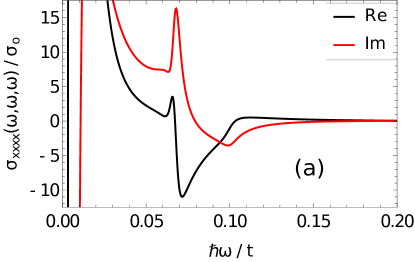
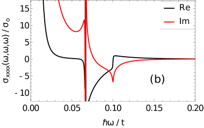
Figure 1: Frequency dependence of the third order nonlinear conductivity of graphene, normalized to $\sigma_{0}=3\,q^{4}a^{2}t^{2}/16\pi\hbar\mu^{4}$ (same normalization used in mikhailov2016quantum ), at zero temperature. The parameters used were: (a) $\mu/t=0.1$, $\gamma/t=0.011$; (b) and $\mu/t=0.1$, $\gamma/t=0.001$. The curves were obtained from a length gauge approach, with the relaxation parameter $\gamma$ introduced via a scattering term in the equation of motion (Eq. 38).

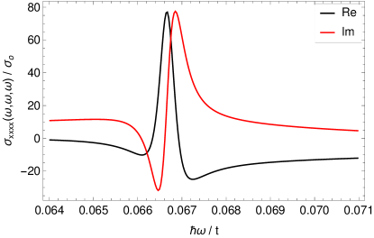
Figure 2: Anomalous feature of the third order nonlinear conductivity of graphene from Fig. 1(b), in a region near the three photon resonance $3\hbar\omega=2\mu$.

Results obtained from the standard length gauge approach are presented in Fig. 1, for frequencies near the Dirac point. In this case, the analytical form of the third order conductivity in the Dirac point approximation was calculated and then plotted. Also, $\gamma$ is introduced via the additional scattering term in the equation of motion (first type of phenomenological treatment described in the previous section), as in Mikhailov’s work mikhailov2016quantum .

These results are in agreement with analogous calculations already in the literature cheng2014third ; mikhailov2016quantum ; cheng2015third , with the strongest feature present at the three photon resonance $3\hbar\omega=2\mu$. In particular, Fig. 1(a) is identical to Fig. 3(b) and Fig. 5 in refs cheng2014third and mikhailov2016quantum , respectively. Fig. 1(b) shows a very anomalous behavior at the resonance, which is always present in a region $\left|3\hbar\omega-2\mu\right|\leq\gamma$ for small but finite $\gamma$. Fig. 2 shows a close-up of this region. This strange feature near resonance is analyzed in detail in mikhailov2016quantum , where it is regarded as a prominent feature of potential interest, since in practice $\gamma$ is always finite. However, a more careful analysis shows that despite the unusual shape of this feature, in the limit $\gamma\rightarrow 0^{+}$, the scattering free result in cheng2014third is indeed obtained (see Appendix C).

To do the same calculations with the velocity gauge approach developed here, we evaluate analytically not the full third order conductivity but only the following functions

$$h_{\textbf{k}ss^{\prime}}^{x}=\frac{a\,\sin\left(\frac{k_{x}a}{2}\right)C_{ss^{\prime}}}{\hbar\sqrt{3+2\cos\left(k_{x}a\right)+4\cos\left(\frac{k_{x}a}{2}\right)\cos\left(\frac{\sqrt{3}k_{y}a}{2}\right)}}$$ (47)

$$h_{\textbf{k}ss^{\prime}}^{xx}=\frac{a^{2}\,\cos\left(\frac{k_{x}a}{2}\right)C_{ss^{\prime}}}{2\hbar^{2}\sqrt{3+2\cos\left(k_{x}a\right)+4\cos\left(\frac{k_{x}a}{2}\right)\cos\left(\frac{\sqrt{3}k_{y}a}{2}\right)}}$$ (48)

$$h_{\textbf{k}ss^{\prime}}^{xxx}=-\frac{a^{2}}{4\hbar^{2}}h_{\textbf{k}ss^{\prime}}^{x}\qquad h_{\textbf{k}ss^{\prime}}^{xxxx}=-\frac{a^{2}}{4\hbar^{2}}h_{\textbf{k}ss^{\prime}}^{xx}$$ (49)

$$C \equiv t$$

$$\times \left[\begin{matrix}2\cos\left(\frac{k_{x}a}{2}\right)+\cos\left(\frac{\sqrt{3}k_{y}a}{2}\right)&\mkern-18.0mu-i\sin\left(\frac{\sqrt{3}k_{y}a}{2}\right)\\ i\sin\left(\frac{\sqrt{3}k_{y}a}{2}\right)&\mkern-18.0mu-2\cos\left(\frac{k_{x}a}{2}\right)+\cos\left(\frac{\sqrt{3}k_{y}a}{2}\right)\end{matrix}\right]$$ (50)

All these analytical functions follow from direct evaluation of the commutators (Eq. 13) using Eqs. 45 and 46. At this point, the expression in Eq. 32 for the nonlinear conductivity (with $n=3$) can be evaluated by numerical integration over the full FBZ. The phenomenology adopted here is the one that follows from adiabatic switching, for the reasons discussed in the previous section.

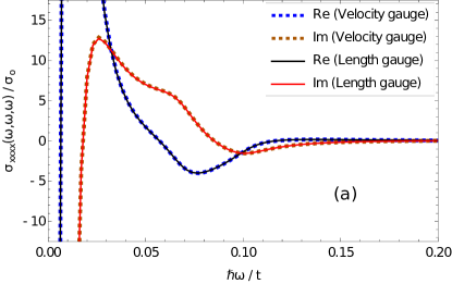
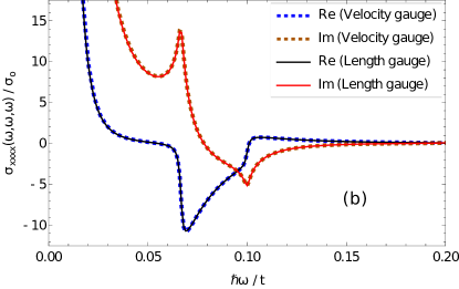
Figure 3: Frequency dependence of the third order nonlinear conductivity of graphene, normalized to $\sigma_{0}=3\,q^{4}a^{2}t^{2}/16\pi\hbar\mu^{4}$ (same normalization used in mikhailov2016quantum ), at zero temperature. The parameters used were: (a) $\mu/t=0.1$, $\gamma/t=0.011$; (b) $\mu/t=0.1$, $\gamma/t=0.001$. The solid curves were obtained from a length gauge approach and the dashed ones from a velocity gauge calculation. The results are identical. The relaxation parameter $\gamma$ was introduced by adiabatic switching, simply replacing $\hbar\omega\rightarrow\hbar\omega+i\gamma$.

The velocity gauge results are in Fig. 3. The curves are markedly different than the ones obtained from the length gauge, especially for large $\gamma$. This should came with no surprise, since a different phenomenological treatment is adopted. To prove that the difference between the two curves is only due to the way the relaxation parameters are introduced, the length gauge calculations were performed again, now with this second type phenomenological treatment (using the third order analogue of Eq. 42) and included in the plots of Fig. 3. The results obtained in the two gauges are identical.

Of course, as we take the relaxation free limit $\gamma\rightarrow 0^{+}$ the results of both phenomenological treatments also coincide. However, for finite $\gamma$ it may lead to some considerably different behavior of the nonlinear conductivity. In particular, we note that in the phenomenology adopted here ($\hbar\omega_{i}\rightarrow\hbar\omega_{i}+i\gamma$), those anomalous features seen in Fig. 1 and discussed in mikhailov2016quantum are not present. Instead, a more plausible smooth curve is seen at the resonances.

As a final remark, we emphasize that the results presented here for the velocity gauge involved a complete two-band tight binding model and an integration over the full FBZ, not an effective Dirac Hamiltonian, as in the case of the length gauge results. This has some consequences. First, it had been suggested that a possible source for the two order of magnitude discrepancy between theoretical and experimental results in graphene could be the use of an effective Hamiltonian cheng2014third . The agreement displayed in Fig. 3 establishes that the Dirac point approximation is valid for the range of frequencies adopted in previous studiescheng2014third ; cheng2015third ; mikhailov2016quantum . Second, the use of complete bands will allow us to proceed towards higher frequencies and study spectral regions where the Dirac Hamiltonian does not give an accurate description.

VII CONCLUSIONS

In summary, a velocity gauge approach to calculations of nonlinear optical conductivities was developed in this work, within the density matrix formalism. It was shown that, contrary to common belief, the results are the same as those from the length gauge, as demanded by gauge invariance. No difficulties come from applying this velocity gauge formalism to finite band models.

The velocity gauge provides an efficient algorithm for computing nonlinear conductivities. The dispersion relation and the Berry connection of a crystal are the prerequisites and define the crystalline system under study. A series of commutators (Eq. 13) can then be analytically computed. From these, the conductivity can be numerically evaluated for any frequencies, temperature, chemical potential, relaxation parameter and to any order, without using any numerical derivatives.

Previously, studies of nonlinear conductivities often involved writing down analytical expressions for the full conductivity. For third order, this already becomes rather cumbersome. Analytically, it is only really tractable for simple effective continuum Hamiltonians (such as the Dirac Hamiltonian). The velocity gauge approach developed here does not have such complications, is easily generalizable to higher orders and is always applied to complete bands. This gauge provide us with a simple yet powerful method to compute the nonlinear optical response functions of crystalline systems.

Appendix A Equivalence of linear responses

As an illustration of the general sum rules implicit in a velocity gauge treatment, the expression for the linear conductivity in the velocity gauge

$$\sigma_{\alpha\beta}^{(1)}(\omega)=\frac{iq^{2}}{\omega}\int\frac{d^{d}\textbf{k}}{(2\pi)^{d}}\sum_{ss^{\prime}}\left(\frac{h_{\textbf{k}ss^{\prime}}^{\beta}\left[h_{\mathbf{k}}^{\alpha},\rho_{\mathbf{k}}^{(0)}\right]_{s^{\prime}s}}{\hbar\omega-\Delta\epsilon_{\textbf{k}s^{\prime}s}}+h_{\textbf{k}ss^{\prime}}^{\beta\alpha}\rho_{\textbf{k}s^{\prime}s}^{(0)}\right)$$ (51)

will be shown to be equivalent to the one obtained from a length gauge approach,

$$\sigma_{\alpha\beta}^{(1)}(\omega)=-iq^{2}\int\frac{d^{d}\textbf{k}}{(2\pi)^{d}}\sum_{ss^{\prime}}\frac{h_{\textbf{k}ss^{\prime}}^{\beta}\left[D_{\mathbf{k}}^{\alpha},\rho_{\mathbf{k}}^{(0)}\right]_{s^{\prime}s}}{\hbar\omega-\Delta\epsilon_{\textbf{k}s^{\prime}s}}$$ (52)

To begin, the Jacobi identity is used to move the covariant derivative to the density matrix

$$\hbar\left[h_{\mathbf{k}}^{\alpha},\rho_{\mathbf{k}}^{(0)}\right] =\left[\left[D_{\mathbf{k}}^{\alpha},H_{0}\right],\rho_{\mathbf{k}}^{(0)}\right]$$

$$=\left[\left[D_{\mathbf{k}}^{\alpha},\rho_{\mathbf{k}}^{(0)}\right],H_{0}\right]+\left[D_{\mathbf{k}}^{\alpha},\left[H_{0},\rho_{\mathbf{k}}^{(0)}\right]\right]$$

$$=\left[\left[D_{\mathbf{k}}^{\alpha},\rho_{\mathbf{k}}^{(0)}\right],H_{0}\right]$$ (53)

where in the last step we took into account that the commutator of two diagonal matrices is zero $\left[H_{0},\rho_{\mathbf{k}}^{(0)}\right]=0$. This leads to

$$\left[h_{\mathbf{k}}^{\alpha},\rho_{\mathbf{k}}^{(0)}\right]_{ss^{\prime}}=\hbar^{-1}\left[D_{\mathbf{k}}^{\alpha},\rho_{\mathbf{k}}^{(0)}\right]_{ss^{\prime}}\Delta\epsilon_{\textbf{k}s^{\prime}s}$$ (54)

The first term in in parenthesis of Eq. 51, dropping the k index for simplicity, becomes

$$\frac{h_{ss^{\prime}}^{\beta}\left[h^{\alpha},\rho^{(0)}\right]_{s^{\prime}s}}{\hbar\omega-\Delta\epsilon_{s^{\prime}s}}= \frac{h_{ss^{\prime}}^{\beta}\,\hbar^{-1}\left[D^{\alpha},\rho^{(0)}\right]_{s^{\prime}s}\Delta\epsilon_{ss^{\prime}}}{\hbar\omega-\Delta\epsilon_{s^{\prime}s}}$$

$$= h_{ss^{\prime}}^{\beta}\,\hbar^{-1}\left[D^{\alpha},\rho^{(0)}\right]_{s^{\prime}s}$$

$$- \frac{\omega\,h_{ss^{\prime}}^{\beta}\left[D^{\alpha},\rho^{(0)}\right]_{s^{\prime}s}}{\hbar\omega-\Delta\epsilon_{s^{\prime}s}}$$ (55)

The second term when replaced in Eq. 51 will give the length gauge result in Eq. 52. The remaining contributions must therefore be zero and form our sum rule,

$$\frac{iq^{2}}{\omega}\int\frac{d^{d}\textbf{k}}{(2\pi)^{d}}\sum_{ss^{\prime}}\left(h_{\mathbf{k}ss^{\prime}}^{\beta}\,\hbar^{-1}\left[D_{\mathbf{k}}^{\alpha},\rho_{\mathbf{k}}^{(0)}\right]_{s^{\prime}s}+h_{\textbf{k}ss^{\prime}}^{\beta\alpha}\rho_{\textbf{k}s^{\prime}s}^{(0)}\right)=0$$ (56)

This can be further simplified through

$$h_{ss^{\prime}}^{\beta\alpha}\equiv\hbar^{-1}\left[D^{\alpha},h^{\beta}\right]_{ss^{\prime}}$$ (57)

to

$$\sum_{ss^{\prime}}\left(h_{ss^{\prime}}^{\beta}\,\hbar^{-1}\left[D^{\alpha},\rho^{(0)}\right]_{s^{\prime}s}+\right. \left.h_{ss^{\prime}}^{\beta\alpha}\rho_{s^{\prime}s}^{(0)}\right)$$ (58)

$$= \hbar^{-1}\sum_{s}\left[D^{\alpha},\,h^{\beta}\rho^{(0)}\right]_{ss}$$ (59)

leading to the form

$$\frac{iq^{2}}{\hbar\omega}\int\frac{d^{d}\textbf{k}}{(2\pi)^{d}}\sum_{s}\left[D_{\mathbf{k}}^{\alpha},h_{\mathbf{k}}^{\beta}\rho_{\mathbf{k}}^{(0)}\right]_{ss}=0$$ (60)

which can be recognized as a particular case of the sum rules identified in the appendix A of ventura2017gauge . The commutator with $D^{\alpha}$ can be broken into two pieces, one involving the Berry connection which is trivially zero (the trace of a proper commutator is always zero) and another involving a conventional derivative,

$$\frac{iq^{2}}{\hbar\omega}\int\frac{d^{d}\textbf{k}}{(2\pi)^{d}}\sum_{s^{\prime}}\frac{\partial}{\partial k_{\alpha}}\left(h_{\textbf{k}ss^{\prime}}^{\beta}\rho_{\textbf{k}s^{\prime}s}^{(0)}\right)=0$$ (61)

This condition is always true since the functions $h$ and $\rho^{(0)}$ are periodic in reciprocal space. The sum rule (and therefore the equivalence between the results in the two gauges) is therefore trivially satisfied as long as the integral is performed over the full FBZ.

Appendix B Expansion of $H_{0}^{A}$ on the vector potential

In our previous paper ventura2017gauge , we discussed in detail the equivalence of the length and velocity gauges in the context of the unperturbed Hamiltonian of Eq. 3. In this appendix, we review this equivalence, using from the start a representation of the crystal Hamiltonian in terms of a set of bands that can be finite.

The representation of the position operator in the Bloch basis blount1962formalisms ; ventura2017gauge requires the thermodynamic limit. We choose the following normalization for the Bloch states

$$\langle\psi_{\mathbf{k}^{\prime}s^{\prime}}|\psi_{\mathbf{k}s}\rangle=\left(2\pi\right)^{d}\delta\left(\mathbf{k}-\mathbf{k}^{\prime}\right)\delta_{ss^{\prime}}$$ (62)

with the corresponding resolution of the identity

$$\sum_{s}\int\frac{d^{d}k}{\left(2\pi\right)^{d}}\left|\psi_{\mathbf{k}s}\right\rangle\left\langle\psi_{\mathbf{k}s}\right|=\bm{\hat{1}}$$ (63)

where the sum over $s$ may be over a finite set of bands. The unperturbed crystal Hamiltonian is

$$H_{0}=\sum_{s^{\prime},s}\int\frac{d^{d}k}{\left(2\pi\right)^{d}}\left|\psi_{\mathbf{k}s}\right\rangle\left[H_{0}\right]_{\mathbf{k}ss^{\prime}}\left\langle\psi_{\mathbf{k}s^{\prime}}\right|$$ (64)

with $\left[H_{0}\right]_{\mathbf{k}ss^{\prime}}=\epsilon_{\mathbf{k}s}\delta_{ss^{\prime}}$, and $\epsilon_{\mathbf{k}s}$ the band energies. The perturbation in the length gauge involves the position operator,

$$H^{E}=H_{0}-q\mathbf{E}(t)\cdot\mathbf{r}$$ (65)

Using Blount’s result for $\mathbf{r}$ in the thermodynamic limit blount1962formalisms , we showed in our previous paper that ventura2017gauge

$$\left\langle\psi_{\mathbf{k}s}\right|\mathbf{r}\left|\psi\right\rangle=\sum_{s^{\prime}}i\mathbf{D}_{\mathbf{k}ss^{\prime}}\langle\psi_{\mathbf{k}s^{\prime}}|\psi\rangle$$ (66)

where the covariant derivative is defined by Eq. 9.

From Eq. 66, we can give the position operator the following representation:

$$\mathbf{r}=\sum_{s,s^{\prime}}\int\frac{d^{d}k}{\left(2\pi\right)^{d}}\left|\psi_{\mathbf{k}s}\right\rangle i\mathbf{D}_{\mathbf{k}ss^{\prime}}\left\langle\psi_{\mathbf{k}s^{\prime}}\right|.$$ (67)

On first inspection, this equation might suggest that this operator is diagonal in Bloch momentum; it is not because of the presence of the gradient with respect to $\mathbf{k}$. Any observable that can be written as a differential operator acting on the wave function in a continuous basis will have a similar representation .

The full single particle Hamiltonian in the length gauge is, therefore,

$$H^{E}=\sum_{s,s^{\prime}}\int\frac{d^{d}k}{\left(2\pi\right)^{d}}\left|\psi_{\mathbf{k}s}\right\rangle\left[\delta_{ss^{\prime}}\epsilon_{\mathbf{k}s}-iq\mathbf{E}(t)\cdot\mathbf{D}_{\mathbf{k}ss^{\prime}}\right]\left\langle\psi_{\mathbf{k}s^{\prime}}\right|$$ (68)

The velocity gauge is obtained by a time dependent unitary transformation,

$$\left|\psi_{A}(t)\right\rangle=S(t)\left|\psi_{E}(t)\right\rangle$$ (69)

$$S(t)=\sum_{s,s^{\prime}}\int\frac{d^{d}k}{\left(2\pi\right)^{d}}\left|\psi_{\mathbf{k}s^{\prime}}\right\rangle\left[e^{-\frac{q}{\hbar}\mathbf{A}(t)\cdot\mathbf{D}_{\mathbf{k}}}\right]_{s^{\prime}s}\left\langle\psi_{\mathbf{k}s}\right|.$$ (70)

The time evolution in this gauge is

$$\left\langle\psi_{\mathbf{k}s}\right|i\hbar\frac{d}{dt}\left|\psi_{A}(t)\right\rangle =\left\langle\psi_{\mathbf{k}s}\right|S(t)\hat{H}_{E}S^{\dagger}(t)\left|\psi_{A}(t)\right\rangle$$

$$+\left\langle\psi_{\mathbf{k}s}\right|i\hbar\frac{dS(t)}{dt}S^{\dagger}(t)\left|\psi_{A}\left(t\right)\right\rangle.$$ (71)

The second term is seen to cancel the scalar potential term in the Hamiltonian,

$$\left\langle\psi_{\mathbf{k}s}\right|i\hbar\frac{dS(t)}{dt}S^{\dagger}(t)\left|\psi_{A}(t)\right\rangle =-i\sum_{s^{\prime}}q\frac{d\mathbf{A}}{dt}\cdot\mathbf{D}_{\mathbf{k}ss^{\prime}}\langle\psi_{\mathbf{k}s^{\prime}}|\psi_{A}(t)\rangle$$

$$=i\sum_{s^{\prime}}q\mathbf{E}(t)\cdot\mathbf{D}_{\mathbf{k}ss^{\prime}}\langle\psi_{\mathbf{k}s^{\prime}}|\psi_{A}(t)\rangle$$ (72)

The velocity gauge Hamiltonian therefore becomes

$$H^{A}=\sum_{s,s^{\prime}}\int\frac{d^{d}k}{\left(2\pi\right)^{d}}\left|\psi_{\mathbf{k}s}\right\rangle H_{\mathbf{k}ss^{\prime}}^{A}\left\langle\psi_{\mathbf{k}s^{\prime}}\right|$$ (73)

with

$$H_{\mathbf{k}ss^{\prime}}^{A}\equiv\sum_{r,r^{\prime}}\left[e^{-\frac{q}{\hbar}\mathbf{A}(t)\cdot\mathbf{D}_{\mathbf{k}}}\right]_{sr}\left[H_{0}\right]_{\mathbf{k}rr^{\prime}}\left[e^{\frac{q}{\hbar}\mathbf{A}(t)\cdot\mathbf{D}_{\mathbf{k}}}\right]_{r^{\prime}s^{\prime}}$$

At this point, we make use of the following identity for any two operators $\hat{B}$ and $\hat{C}$,

$$e^{\hat{C}}\,\hat{B}\,e^{-\hat{C}}=\hat{B}+\left[\hat{C},\hat{B}\right]+\frac{1}{2!}\left[\hat{C},\left[\hat{C},\hat{B}\right]\right]+\dots$$ (74)

and apply it to Eq. 73 with $\hat{B}=H_{0}$ and $\hat{C}=-\frac{q}{\hbar}\mathbf{A}(t)\cdot\mathbf{D}_{\mathbf{k}}$, to get

$$H_{\mathbf{k}ss^{\prime}}^{A}= \sum_{n=0}^{\infty}\frac{(-q)^{n}\,A_{\alpha_{1}}(t)\dots A_{\alpha_{n}}(t)}{\hbar^{n}\,n!}$$

$$\times \left[D_{\mathbf{k}}^{\alpha_{n}},\left[\dots,\left[D_{\mathbf{k}}^{\alpha_{1}},H_{0}\right]\right]...\right]_{ss^{\prime}}$$

$$= \epsilon_{\mathbf{k}s}\delta_{ss^{\prime}}$$

$$+ \sum_{n=1}^{\infty}\frac{(-q)^{n}\,A_{\alpha_{1}}(t)\dots A_{\alpha_{n}}(t)}{\hbar^{n}\,n!}$$

$$\times \left[D_{\mathbf{k}}^{\alpha_{n}},\left[\dots,\left[D_{\mathbf{k}}^{\alpha_{1}},H_{0}\right]\right]...\right]_{ss^{\prime}}$$ (75)

Appendix C Brief note on a phenomenological feature

In mikhailov2016quantum , Mikhailov pointed out that the feature observed in Fig. 2 was due mainly to a term of the form

$$\sim\imaginary\frac{\gamma}{(3\hbar\omega-2\mu+i\gamma)^{2}}$$ (76)

In the limit $\gamma\rightarrow 0$, this should be considered a distribution, to be integrated over frequency. One knows that

$$\lim_{\gamma\to 0}\imaginary\frac{1}{3\hbar\omega-2\mu+i\gamma}$$ (77)

corresponds to a Dirac delta function, so one may ask to what distribution corresponds Eq. 76. Since we can write

$$\lim\limits_{\gamma\rightarrow 0}\imaginary\frac{\gamma}{(3\hbar\omega-2\mu+i\gamma)^{2}}= \frac{-1}{3\hbar}\lim\limits_{\gamma\rightarrow 0}\imaginary\partial_{\omega}\frac{\gamma}{3\hbar\omega-2\mu+i\gamma}$$ (78)

upon integration with a test function $f(\omega)$, we obtain a contribution $\propto\lim\limits_{\gamma\rightarrow 0}\gamma\,f^{\prime}(2\mu/3\hbar)$ which is always zero. In this limit, the term in Eq. 76 has no weight at all. It will not show up in an integration over $\omega$. Similar remarks can be made concerning the other resonances in the nonlinear conductivity, computed via the standard phenomenological approach; this is how the two phenomenologies discussed in Section V yield different results for any finite $\gamma,$ yet, nevertheless, become identical in the $\gamma\to 0^{+}$ limit.

References

• [1] Yuen-Ron Shen. The principles of nonlinear optics. New York, Wiley-Interscience, 1984, 575 p., 1984.
• [2] JE Sipe and Ed Ghahramani. Nonlinear optical response of semiconductors in the independent-particle approximation. Physical Review B, 48(16):11705, 1993.
• [3] Claudio Aversa and JE Sipe. Nonlinear optical susceptibilities of semiconductors: Results with a length-gauge analysis. Physical Review B, 52(20):14636, 1995.
• [4] GB Ventura, DJ Passos, JMB Lopes dos Santos, JM Viana Parente Lopes, and NMR Peres. Gauge covariances and nonlinear optical responses. Physical Review B, 96(3):035431, 2017.
• [5] VN Genkin and PM Mednis. Contribution to the theory of nonlinear effects in crystals with account taken of partially filled bands. Sov. Phys. JETP, 27:609, 1968.
• [6] James LP Hughes and JE Sipe. Calculation of second-order optical response in semiconductors. Physical Review B, 53(16):10751, 1996.
• [7] JE Sipe and AI Shkrebtii. Second-order optical response in semiconductors. Physical Review B, 61(8):5337, 2000.
• [8] Ibraheem Al-Naib, JE Sipe, and Marc M Dignam. High harmonic generation in undoped graphene: Interplay of inter-and intraband dynamics. Physical Review B, 90(24):245423, 2014.
• [9] F Hipolito, Thomas G Pedersen, and Vitor M Pereira. Nonlinear photocurrents in two-dimensional systems based on graphene and boron nitride. Physical Review B, 94(4):045434, 2016.
• [10] EI Blount. Formalisms of band theory. Solid state physics, 13:305–373, 1962.
• [11] JL Cheng, N Vermeulen, and JE Sipe. Dc current induced second order optical nonlinearity in graphene. Optics express, 22(13):15868–15876, 2014.
• [12] Jin Luo Cheng, Nathalie Vermeulen, and JE Sipe. Third-order nonlinearity of graphene: Effects of phenomenological relaxation and finite temperature. Physical Review B, 91(23):235320, 2015.
• [13] Fred Nastos, Bernd Olejnik, Karlheinz Schwarz, and JE Sipe. Scissors implementation within length-gauge formulations of the frequency-dependent nonlinear optical response of semiconductors. Physical Review B, 72(4):045223, 2005.
• [14] Claudio Aversa, JE Sipe, M Sheik-Bahae, and EW Van Stryland. Third-order optical nonlinearities in semiconductors: The two-band model. Physical Review B, 50(24):18073, 1994.
• [15] K Rzazewski and Robert W Boyd. Equivalence of interaction hamiltonians in the electric dipole approximation. Journal of modern optics, 51(8):1137–1147, 2004.
• [16] Alireza Taghizadeh, F Hipolito, and TG Pedersen. Linear and nonlinear optical response of crystals using length and velocity gauges: Effect of basis truncation. arXiv preprint arXiv:1710.01300, 2017.
• [17] Kuljit S Virk and JE Sipe. Semiconductor optics in length gauge: A general numerical approach. Physical Review B, 76(3):035213, 2007.
• [18] JL Cheng, Nathalie Vermeulen, and JE Sipe. Third order optical nonlinearity of graphene. New Journal of Physics, 16(5):053014, 2014.
• [19] Michael V Berry. Quantal phase factors accompanying adiabatic changes. In Proceedings of the Royal Society of London A: Mathematical, Physical and Engineering Sciences, volume 392, pages 45–57. The Royal Society, 1984.
• [20] Di Xiao, Ming-Che Chang, and Qian Niu. Berry phase effects on electronic properties. Reviews of modern physics, 82(3):1959, 2010.
• [21] Sergey A Mikhailov. Quantum theory of the third-order nonlinear electrodynamic effects of graphene. Physical Review B, 93(8):085403, 2016.
• [22] JL Cheng, N Vermeulen, and JE Sipe. Second order optical nonlinearity of graphene due to electric quadrupole and magnetic dipole effects. Scientific Reports, 7, 2017.
• [23] MM Glazov and SD Ganichev. High frequency electric field induced nonlinear effects in graphene. Physics Reports, 535(3):101–138, 2014.
• [24] SA Mikhailov. Non-linear electromagnetic response of graphene. EPL (Europhysics Letters), 79(2):27002, 2007.
• [25] SA Mikhailov. Nonperturbative quasiclassical theory of the nonlinear electrodynamic response of graphene. Physical Review B, 95(8):085432, 2017.
• [26] A Marini, JD Cox, and FJ García de Abajo. Theory of graphene saturable absorption. Physical Review B, 95(12):125408, 2017.
• [27] NMR Peres, Yu V Bludov, Jaime E Santos, Antti-Pekka Jauho, and MI Vasilevskiy. Optical bistability of graphene in the terahertz range. Physical Review B, 90(12):125425, 2014.
• [28] AH Castro Neto, F Guinea, Nuno MR Peres, Kostya S Novoselov, and Andre K Geim. The electronic properties of graphene. Reviews of modern physics, 81(1):109, 2009.