Performance Analysis of Approximate Message Passing for Distributed Compressed Sensing

Abstract

bamp is an efficient method in compressed sensing that is nearly optimal in the mmse sense. Multiple measurement vector (MMV)-bamp performs joint recovery of multiple vectors with identical support and accounts for correlations in the signal of interest and in the noise. In this paper, we show how to reduce the complexity of vector bamp via a simple joint decorrelation (diagonalization) transform of the signal and noise vectors, which also facilitates the subsequent performance analysis. We prove that the corresponding se is equivariant with respect to the joint decorrelation transform and preserves diagonality of the residual noise covariance for the bg prior. We use these results to analyze the dynamics and the mse performance of bamp via the replica method, and thereby understand the impact of signal correlation and number of jointly sparse signals. Finally, we evaluate an application of MMV-BAMP for single-pixel imaging with correlated color channels and thereby explore the performance gain of joint recovery compared to conventional BAMP reconstruction as well as group lasso.

mmse

I Introduction

cs is a signal processing technique aiming at recovering a high-dimensional sparse vector from a (noisy) system of linear equations [1, 2]. Joint sparsity refers to multiple vectors having the same support set, whose cardinality is typically much lower than the signal dimension. There are two prominent cs scenarios [3, 4] in the context of joint sparsity: (i) the mmv problem, where the measurement matrices are identical, and (ii) the dcs problem, where the measurement matrices are independent. Joint sparsity arises in a number of real-world scenarios, e.g., when multiple sensors or antennas observe the same signal corrupted by different channels and noise (e.g., [3, 4]). A prime example is radio frequency identification where the observed vectors are the received signals at different antennas (of the same receiver) [5]. Additionally, typical applications are magnetic resonance imaging [6], distributed networks [7], wireless communications [5], and direction of arrival estimation [8].

In this work, we investigate an amp solution for joint sparse recovery when there is possible correlation between the signals (and the noise). We then evaluate this algorithm in the context of single-pixel color imaging [9]. In particular, we show the potential of joint recovery that exploits the correlation between the red, green, blue (RGB) color intensity channels.

I-A Related Work

Several methods for jointly sparse recovery have been proposed in the literature [3, 10, 11, 12, 13, 14, 7, 15, 16, 17, 18, 19]. amp was introduced in [20, 21, 22] as a large system relaxation of loopy belief propagation to solve a random linear system with sparsity constraint. Scalar bamp, its Bayesian version [23, 24], uses the signal prior explicitly and is an efficient approximate mmse estimator. The turbo bamp methods in [14, 15, 16], and their generalization in [25] for clustered sparse signals, improve the recovery performance by exchanging extrinsic information about the current support estimate in each message passing iteration. In [17, 18, 26], joint sparsity is directly enforced by an appropriate vector estimator (denoiser) function for the bg prior.

The se formalism developed in [21, 22, 27] analytically predicts the recovery performance of (B)amp algorithms. se was employed to analyze bamp for joint sparsity with a vector estimator and to point out the difference between the dcs and mmv scenarios in [18]. Recent works rigorously prove the se for non-separable non-linearities [28] and a class of sliding-window denoisers [29] with Gaussian i.i.d. measurement matrices. Furthermore, the se of the Vector AMP has been derived for a large class of right orthogonally invariant random sensing matrices [30]. (We highlight that the acronym Vector AMP should not to be confused with the vector-prior version of BAMP, considered in this paper for the MMV/DCS problems.)

In [26], the replica method (a statistical physics tool for large disordered systems) is used to calculate the mmse of the cs measurement (note that [26] refers to mmv and dcs as MMV-2 and MMV-1, respectively). The replica trick non-rigorously simplifies the high-dimensional integral for the mmse of the Bayesian estimator of the cs channel, thereby leading to the free energy as a function of the mse. The local maxima in the free energy function correspond to stable fixed points of bp and bamp and thus predict the expected mse of bamp. The replica analysis in [26] is performed for the bg signal prior with uncorrelated isotropic unitary signal and uncorrelated isotropic Gaussian noise distribution, i.e., with a single noise parameter.

I-B Contributions

We consider the vector-prior bamp algorithm for the dcs and mmv problems, which uses an appropriate vector mmse estimator function and Onsager correction term to exploit joint sparsity structure, the signal distribution, and the noise covariance. We provide an analytical performance prediction for the bamp algorithm with a bg signal prior with arbitrary signal and noise correlation by (i) incorporating a linear joint decorrelation of the measurements, (ii) showing the equivariance of Vbamp w.r.t. invertible linear transformations, (iii) extending the replica analysis from [26] to arbitrary diagonal noise covariance matrices.

In particular, the joint decorrelation yields a simpler equivalent measurement model with diagonal signal and noise covariance matrix (under mild conditions, one of the covariance matrices can be made the identity matrix). The simplified model naturally provides the measurement snr of each signal vector and substantially reduces the complexity of the Vbamp iterations. We further show that the Vbamp algorithm is equivariant to invertible linear transformations, thus, it preserves its properties across iterations in the transformed domain and delivers a result equivalent to that obtained with the original measurements and covariance parameters. For the widely used bg prior, we prove that the Vbamp iterations (and the corresponding se) preserve the diagonal structure of the (effective) noise covariance, thus implying that a $B$-dimensional state (instead of $B(B+1)/2$ dimensions) is sufficient and that every mmv problem can be transformed into an equivalent dcs problem. Finally, we extend the replica analysis in [26] to the case of anisotropic noise (i.e., $B$ noise parameters instead of just $1$). The replica analysis yields the $B$ measurement-wise mse of the Vbamp estimate in its fixed points. We use both real-world and synthetic images to compare MMV-BAMP to state-of-the-art scalar recovery algorithms and to joint sparsity-aware algorithms in the context of single-pixel color imaging.

I-C Outline

The remainder of this paper is organized as follows. In Section II, we discuss the Vbamp algorithm, the estimator function for the multivariate bg signal prior, and the multivariate state evolution of Vbamp. In Section III, the joint decorrelation of the signal and the noise vectors is investigated in the context of Vbamp and state evolution; the multivariate bg signal prior is studied as special case. In Section IV, we present the multivariate free energy formula for arbitrary diagonal noise covariance matrices (the details of the replica analysis are relegated to the appendix). Section V provides a qualitative discussion and open questions regarding the effects of signal correlation and the increasing number of jointly sparse vectors on the dynamics of Vbamp. Section VI evaluates the MMV-BAMP algorithm on a simplified single pixel imaging problem, highlighting the benefits of exploiting signal correlation across channels. We close with conclusions in Section VII.

I-D Notation

Uppercase (lowercase) boldface letters denote matrices (vectors), and serif letters denote random quantities. For a matrix $\mathbf{A}$ (vector $\mathbf{a}$), $\mathbf{A}_{i}$ ($a_{i}$) denotes its $i$th row ($i$th entry) and $\mathbf{a}_{i}$ its $i$th column. The all zero matrix and the identity matrix of dimension $M\times N$ are denoted by $\mathbf{0}_{M\times N}$ and $\mathbf{I}_{M\times N}$, respectively (we omit the subscript if the dimensions are clear from the context). The Dirac delta (generalized) function is $\delta(\mathbf{x})$. The normal distribution with mean $\bm{\mu}$ and covariance matrix $\bm{\Sigma}$ is denoted by $\mathcal{N}(\bm{\mu},\bm{\Sigma})$ and $\mathcal{N}(\mathbf{x};\bm{\mu},\bm{\Sigma})$ denotes the value of this normal pdf at $\mathbf{x}$. The outer product of a column vector $\mathbf{x}$ with itself is denoted by $\bm{\langle}\mathbf{x}\bm{\rangle}=\mathbf{x}\mathbf{x}^{T}$. For a vector $\mathbf{x}=(x_{1},\ldots,x_{B})^{T}$, $\operatorname{diag}(\mathbf{x})$ and $\operatorname{diag}(x_{1},\ldots,x_{B})$ denote the diagonal matrix whose $i$th diagonal element equals $x_{i}$. For a matrix $\mathbf{X}$, $D(\mathbf{X})$ is the diagonal matrix whose diagonal is identical to that of $\mathbf{X}$, i.e., $D(\cdot)$ is the orthogonal projection that zeros the off-diagonal elements. The Kronecker product of two matrices is denoted by $\otimes$.

II BAMP with Vector Denoiser

II-A Measurement Model

We consider the measurement model

$$\mathbf{y}(b)=\mathbf{A}(b)\mathbf{x}(b)+\mathbf{w}(b)\,,$$ (1)

with $\mathbf{y}(b)\in\mathbb{R}^{M}$, $\mathbf{x}(b)\in\mathbb{R}^{N}$, $\mathbf{w}(b)\in\mathbb{R}^{M}$, and $\mathbf{A}(b)\in\mathbb{R}^{M\times N}$, for $b=1,\ldots,B$. We denote the measurement rate by $R={M}/{N}$. We assume that the measurement matrices $\mathbf{A}(b)$ are realizations of Gaussian or Rademacher random matrices [31] with normalized columns. If the measurement matrices $\mathbf{A}(b)$ are identical (i.e., $\mathbf{A}(b)=\mathbf{A}$, $b=1,\dots,B$) we have an mmv scenario; if they are mutually independent then we have a dcs scenario. We define the length-$B$ column vectors

$$\vec{\mathbf{x}}_{n} =(x_{n}(1),\ldots,x_{n}(B))^{T},$$

$$\vec{\mathbf{y}}_{m} =(y_{m}(1),\ldots,y_{m}(B))^{T},$$ (2)

$$\vec{\mathbf{w}}_{m} =(w_{m}(1),\ldots,w_{m}(B))^{T}$$

(similar notation will be used throughout the paper). Joint sparsity (cf. JSM-2 in [4]) with sparsity (or nonzero probability) $\epsilon$ requires that $\vec{\mathbf{x}}_{n}=\mathbf{0}$ with probability $1-\epsilon$ and $\vec{\mathbf{x}}_{n}\neq\mathbf{0}$ with probability $\epsilon$. In this work, we focus on signals with multivariate bg pdf, i.e.,

$$f_{\vec{\bm{\mathsf{x}}}_{n}}(\vec{\mathbf{x}}_{n})=f_{\vec{\bm{\mathsf{x}}}}(\vec{\mathbf{x}}_{n})=(1-\epsilon)\,\delta(\vec{\mathbf{x}}_{n})+\epsilon\,\mathcal{N}(\vec{\mathbf{x}}_{n};\mathbf{0},\bm{\Sigma}_{\vec{\bm{\mathsf{x}}}}),$$ (3)

iid over $n$; here, $\bm{\Sigma}_{\vec{\bm{\mathsf{x}}}}$ is the covariance matrix of $\vec{\mathbf{x}}_{n}$ given that it is non-zero vector. The additive noise in (1) is assumed to be iid Gaussian over $m$ with zero mean and covariance $\bm{\Sigma}_{\vec{\bm{\mathsf{w}}}}$,

$$\vec{\bm{\mathsf{w}}}_{m}\sim\mathcal{N}(\mathbf{0},\bm{\Sigma}_{\vec{\bm{\mathsf{w}}}})\,.$$ (4)

II-B Vector-prior BAMP for MMV/DCS

Algorithm 1 Vbamp for MMV/DCS

1:input: $\mathbf{y}(b)$, $\mathbf{A}(b)$, $\bm{\Sigma}_{\vec{\bm{\mathsf{x}}}}$, $\varepsilon$, $t_{\max}$, $\varepsilon_{\mathrm{tol}}$

2:$t=0$, $\hat{\vec{\mathbf{x}}}_{n}^{t}=\mathbf{0}_{B\times 1}$, $\vec{\mathbf{r}}_{m}^{t}=\vec{\mathbf{y}}_{m}$, $\forall m,n$

3:do

4:     $t\leftarrow t+1$

5:     $\mathbf{u}^{t-1}(b)=\hat{\mathbf{x}}^{t-1}(b)+\mathbf{A}(b)^{T}\mathbf{r}^{t-1}(b)$, $\forall b$

6:     $\bm{\Sigma}_{\vec{\bm{\mathsf{v}}}}^{t-1}=\begin{cases}{\bm{\Sigma}_{\vec{r}}^{t-1}}&\mbox{ for MMV}\\ D\big{(}{\bm{\Sigma}_{\vec{r}}^{t-1}}\big{)}&\mbox{ for DCS}\end{cases}$

7:     $\hat{\vec{\mathbf{x}}}_{n}^{t}=F(\vec{\mathbf{u}}_{n}^{t-1};\bm{\Sigma}_{\vec{\bm{\mathsf{v}}}}^{t-1})$, $\forall n$

8:     $\vec{\mathbf{r}}_{m}^{t}=\vec{\mathbf{y}}_{m}-\big{(}\mathbf{A}(1)\hat{\mathbf{x}}^{t}(1),\ldots,\mathbf{A}(B)\hat{\mathbf{x}}^{t}(B)\big{)}_{m}\hskip 42.67912pt$           $\phantom{=}+\frac{1}{M}\sum_{n=1}^{N}F^{\prime}(\vec{\mathbf{u}}_{n}^{t-1};\bm{\Sigma}_{\vec{\bm{\mathsf{v}}}}^{t-1})\vec{\mathbf{r}}_{m}^{t}$, $\forall m$

9:while $\sum_{b=1}^{B}\left\|\hat{\mathbf{x}}^{t}(b)\!-\!\hat{\mathbf{x}}^{t-1}(b)\right\|^{2}_{2}\!>\!\varepsilon_{\mathrm{tol}}\sum_{b=1}^{B}\left\|\hat{\mathbf{x}}^{t-1}(b)\right\|^{2}_{2}$ and $t<t_{\max}$

10:return $\hat{\mathbf{x}}(b)=\hat{\mathbf{x}}^{t}(b)$, $\forall b$

The Vbamp method for joint sparse recovery of $\mathbf{x}(b)$, $b=1,\dots,B$, [19, 17] is summarized in Algorithm 1 (superscript $t$ indicates the iteration index). Note that scalar Vbamp (i.e., when $B=1$) is a special case of Algorithm 1 where mmv and dcs are equivalent. The vector-prior BAMP follows similar steps as ordinary scalar bamp [20, 23, 24, 21, 22, 27]. According to the decoupling principle [24], which holds in the asymptotic regime where $M,N\rightarrow\infty$ while $\frac{M}{N}=R$, the Vbamp algorithm decouples the cs measurements (1) according to

$$\vec{\mathbf{u}}_{n}^{t}=\vec{\mathbf{x}}_{n}+\vec{\mathbf{v}}_{n}^{t},$$ (5)

where the effective noise vector is distributed as ${\vec{\bm{\mathsf{v}}}_{n}^{t}\sim\mathcal{N}(\mathbf{0},\bm{\Sigma}_{\vec{\bm{\mathsf{v}}}}^{t})}$. The effective noise covariance is estimated via the empirical covariance $\bm{\Sigma}_{\vec{r}}^{t}=\operatorname{Cov}\!\left\{\vec{\mathbf{r}}_{m}^{t-1}\right\}$ from vectors $\vec{\mathbf{r}}_{m}^{t-1}$ in line 6 of Algorithm 1. It has been shown in [18] that in the dcs scenario only the diagonal entries of the covariance matrix are retained due to the mixing effected by the $B$ mutually independent measurement matrices. In the following, we will simplify notation by occasionally dropping the indices $t$ and $n$.

The vector denoiser in Vbamp (line 7 of Algorithm 1) amounts to a vector mmse estimator of $\vec{\mathbf{x}}_{n}$ given the decoupled measurements $\vec{\mathbf{u}}_{n}$. Using Bayes’ theorem, the denoiser can be written as:

$$F(\vec{\mathbf{u}};\bm{\Sigma}_{\vec{\bm{\mathsf{v}}}}) =\operatorname{E}_{\vec{\bm{\mathsf{x}}}}\left\{\vec{\bm{\mathsf{x}}}\mid\vec{\bm{\mathsf{u}}}=\vec{\mathbf{u}};\bm{\Sigma}_{\vec{\bm{\mathsf{v}}}}\right\}$$ (6)

$$=\frac{\int_{\mathbb{R}^{B}}\vec{\mathbf{z}}\,\mathcal{N}(\vec{\mathbf{u}};\vec{\mathbf{z}},\bm{\Sigma}_{\vec{\bm{\mathsf{v}}}})f_{\vec{\mathbf{x}}}(\vec{\mathbf{z}})\,d\vec{\mathbf{z}}}{\int_{{\mathbb{R}^{B}}}\mathcal{N}(\vec{\mathbf{u}};\vec{\mathbf{z}},\bm{\Sigma}_{\vec{\bm{\mathsf{v}}}})f_{\vec{\mathbf{x}}}(\vec{\mathbf{z}})\,d\vec{\mathbf{z}}}\,,$$

where the covariance of the effective noise is $\bm{\Sigma}_{\vec{\bm{\mathsf{v}}}}=\bm{\Sigma}_{\vec{r}}$ (mmv) or $\bm{\Sigma}_{\vec{\bm{\mathsf{v}}}}=D(\bm{\Sigma}_{\vec{r}})$ (dcs). For the multivariate bg prior (3), the vector denoiser becomes

$$F(\vec{\mathbf{u}};\bm{\Sigma}_{\vec{\bm{\mathsf{v}}}})=\mathbf{W}\vec{\mathbf{u}}\qquad\text{with }\;\mathbf{W}=\frac{F_{N}(\vec{\mathbf{u}};\bm{\Sigma}_{\vec{\bm{\mathsf{v}}}})}{F_{D}(\vec{\mathbf{u}};\bm{\Sigma}_{\vec{\bm{\mathsf{v}}}})}\bm{\Sigma}_{\vec{\bm{\mathsf{x}}}}\bm{\Sigma}_{\vec{\bm{\mathsf{u}}}}^{-1}.$$ (7)

Here, $\bm{\Sigma}_{\vec{\bm{\mathsf{u}}}}=\bm{\Sigma}_{\vec{\bm{\mathsf{x}}}}+\bm{\Sigma}_{\vec{\bm{\mathsf{v}}}}$ and

$$F_{N}(\vec{\mathbf{u}};\bm{\Sigma}_{\vec{\bm{\mathsf{v}}}}) =\epsilon\,\mathcal{N}(\vec{\mathbf{u}};\mathbf{0},\bm{\Sigma}_{\vec{\bm{\mathsf{u}}}}),$$ (8)

$$F_{D}(\vec{\mathbf{u}};\bm{\Sigma}_{\vec{\bm{\mathsf{v}}}}) =(1-\epsilon)\,\mathcal{N}(\vec{\mathbf{u}};\mathbf{0},\bm{\Sigma}_{\vec{\bm{\mathsf{v}}}})+\epsilon\,\mathcal{N}(\vec{\mathbf{u}};\mathbf{0},\bm{\Sigma}_{\vec{\bm{\mathsf{u}}}})$$

The denoiser (7) consists of a multivariate Gaussian Wiener estimator followed by a joint shrinkage operation.

The Vbamp residual is computed in line 8 of Algorithm 1. As in the original amp derivation [23], the Onsager correction term for the residual $\vec{\mathbf{y}}_{m}-\big{(}\mathbf{A}(1)\hat{\mathbf{x}}(1),\ldots,\mathbf{A}(B)\hat{\mathbf{x}}(B)\big{)}_{m}$ is computed via the derivative of the estimator. In the asymptotic regime, the Onsager term

$$\frac{1}{M}\sum_{n=1}^{N}F^{\prime}(\vec{\mathbf{u}}_{n};\bm{\Sigma}_{\vec{\bm{\mathsf{v}}}})\,\vec{\mathbf{r}}_{m}$$ (9)

renders the decoupled measurement vectors $\vec{\mathbf{u}}_{n}$ Gaussian with mean $\vec{\mathbf{x}}_{n}$ and covariance $\bm{\Sigma}_{\vec{\bm{\mathsf{v}}}}$ [19, 26]. Here, the Jacobian matrix $F^{\prime}(\vec{\mathbf{u}};\bm{\Sigma}_{\vec{\bm{\mathsf{v}}}})={dF(\vec{\mathbf{u}};\bm{\Sigma}_{\vec{\bm{\mathsf{v}}}})}/{d\vec{\mathbf{u}}^{T}}$ of the estimator $F(\vec{\mathbf{u}};\bm{\Sigma}_{\vec{\bm{\mathsf{v}}}})$ is given by

$$F^{\prime}(\vec{\mathbf{u}};\bm{\Sigma}_{\vec{\bm{\mathsf{v}}}})\!=\!\mathbf{W}\!-\!\left(1\!-\!\frac{F_{N}(\vec{\mathbf{u}};\bm{\Sigma}_{\vec{\bm{\mathsf{v}}}})}{F_{D}(\vec{\mathbf{u}};\bm{\Sigma}_{\vec{\bm{\mathsf{v}}}})}\right)\mathbf{W}\vec{\mathbf{u}}_{n}\vec{\mathbf{u}}_{n}^{T}(\bm{\Sigma}_{\vec{\bm{\mathsf{u}}}}^{-1}-\bm{\Sigma}_{\vec{\bm{\mathsf{v}}}}^{-1})\,.$$ (10)

The algorithm runs until the relative change in the estimated signal is below a certain threshold $\varepsilon_{\mathrm{tol}}$ or the maximum number of iterations $t_{\max}$ is reached. Compared to scalar bamp, the vector Vbamp algorithm involves the following crucial modifications:

• a multivariate prior (possibly with joint sparsity structure and correlation);

• the estimator acts on vectors rather than scalars (6) and both correlated signal and correlated additive noise are taken into consideration (more precisely, the full signal and noise vector pdf is taken into account);

• an Onsager term obtained as the sum of Jacobian matrices (cf. (9)).

II-C State Evolution

se was originally proposed in [20] for scalar (B)AMP and extended to the mmv and dcs scenarios (e.g., in [18]); it allows to characterize analytically the expected behavior of Vbamp (note that the Onsager term in [18] is flawed even though the multivariate se is correct). In particular, the se equation predicts the evolution of the effective noise covariance (the state) for any signal prior $f_{\vec{\bm{\mathsf{x}}}}(\vec{\mathbf{x}}_{n})$ as

$$\bm{\Sigma}_{\vec{\bm{\mathsf{v}}}}^{t+1}=\begin{cases}\bm{\Sigma}_{\vec{\bm{\mathsf{w}}}}+\frac{1}{R}\operatorname{E}_{\vec{\bm{\mathsf{x}}},\vec{\bm{\mathsf{v}}}}\left\{\bm{\langle}\mathbf{e}(\vec{\bm{\mathsf{x}}},\vec{\bm{\mathsf{v}}})\bm{\rangle}\right\}&\mbox{for MMV},\\ D\!\left(\bm{\Sigma}_{\vec{\bm{\mathsf{w}}}}+\frac{1}{R}\operatorname{E}_{\vec{\bm{\mathsf{x}}},\vec{\bm{\mathsf{v}}}}\left\{\bm{\langle}\mathbf{e}(\vec{\bm{\mathsf{x}}},\vec{\bm{\mathsf{v}}})\bm{\rangle}\right\}\right)&\mbox{for DCS},\end{cases}$$ (11)

where $\mathbf{e}(\vec{\bm{\mathsf{x}}},\vec{\bm{\mathsf{v}}})=F(\vec{\bm{\mathsf{x}}}+\vec{\bm{\mathsf{v}}};\bm{\Sigma}_{\vec{\bm{\mathsf{v}}}}^{t})-\vec{\bm{\mathsf{x}}}$ is the error achieved by the mmse estimator $F(\vec{\mathbf{u}};\bm{\Sigma}_{\vec{\bm{\mathsf{v}}}}^{t})$ and $\vec{\bm{\mathsf{v}}}\sim\mathcal{N}(\mathbf{0},\bm{\Sigma}_{\vec{\bm{\mathsf{v}}}}^{t})$. The state in the mmv scenario is in general $B(B+1)/2$ dimensional (since the covariance matrix is symmetric). From (11), the mse prediction directly follows as

$$\operatorname{Cov}\{\vec{\mathbf{u}}^{t}_{n}-\vec{\mathbf{x}}_{n}\} =\bm{\Sigma}_{\vec{\bm{\mathsf{v}}}}^{t},$$

$$\widehat{\mathrm{MSE}}{}^{t}(b) =R\,(\bm{\Sigma}_{\vec{\bm{\mathsf{v}}}}^{t}-\bm{\Sigma}_{\vec{\bm{\mathsf{w}}}})_{b,b},$$

with the mse per channel being defined as

$$\mathrm{MSE}^{t}(b)=\frac{1}{N}\|\hat{\mathbf{x}}^{t}(b)-\mathbf{x}(b)\|_{2}^{2}.$$

III Diagonalized Vector-prior BAMP

III-A Joint Diagonalization for MMV

Algorithm 2 joint diagonalization transformation

1:Given $\bm{\Sigma}_{\vec{\bm{\mathsf{x}}}},\bm{\Sigma}_{\vec{\bm{\mathsf{w}}}}$

2:      find $\mathbf{P}$ such that $\mathbf{P}\mathbf{P}^{T}=\bm{\Sigma}_{\vec{\bm{\mathsf{w}}}}$

3:      $\mathbf{G}=\mathbf{P}^{-1}\bm{\Sigma}_{\vec{\bm{\mathsf{x}}}}\mathbf{P}^{-T}$

4:      find eigendecomposition $\mathbf{Q}\bm{\Lambda}\mathbf{Q}^{T}=\mathbf{G}$

5:      $\mathbf{T}=\bm{\Lambda}^{-1/2}\mathbf{Q}^{T}\mathbf{P}^{-1}$

The Vbamp algorithm in Section II-B can deal with arbitrary signal and noise correlations $\bm{\Sigma}_{\vec{\bm{\mathsf{x}}}}$ and $\bm{\Sigma}_{\vec{\bm{\mathsf{w}}}}$, which in general results in a nondiagonal $\bm{\Sigma}_{\vec{\bm{\mathsf{v}}}}^{t}$ in the mmv scenario. In the decoupled measurements $\vec{\mathbf{u}}=\vec{\mathbf{x}}+\vec{\mathbf{v}}$, it means that there are $\mathcal{O}(B^{2})$ snr relations and $B(B+1)/2$ states: each $\mathsf{x}_{n}(b)$ correlates with all $\mathsf{x}_{n}(b^{\prime})$, $b^{\prime}\in\{1,\ldots,B\}\setminus\{b\}$, and it is influenced simultaneously by all effective noise components $\mathsf{v}(b^{\prime})$, $b^{\prime}\in\{1,\ldots,B\}$.

Under the assumption that the covariance matrices $\bm{\Sigma}_{\vec{\bm{\mathsf{x}}}}$ and $\bm{\Sigma}_{\vec{\bm{\mathsf{w}}}}$ are full rank and using the fact that covariance matrices are symmetric and positive definite and [32, Thm. 7.6.1.], there exists a nonsingular (but generally non-orthogonal) matrix $\mathbf{T}$ that simultaneously diagonalizes the covariance matrices of the signal $\vec{\mathbf{x}}$ and the noise $\vec{\mathbf{w}}$. The computation of $\mathbf{T}$ is described in Algorithm 2. In the transformed model

$$\tilde{\vec{\mathbf{y}}}_{m}=\mathbf{T}\vec{\mathbf{y}}_{m},\quad\tilde{\vec{\mathbf{x}}}_{n} =\mathbf{T}\vec{\mathbf{x}}_{n},\quad\tilde{\vec{\mathbf{w}}}_{m}=\mathbf{T}\vec{\mathbf{w}}_{m},$$ (12)

we thus have

$$\bm{\Sigma}_{\tilde{\vec{\bm{\mathsf{x}}}}} =\mathbf{T}\bm{\Sigma}_{\vec{\bm{\mathsf{x}}}}\mathbf{T}^{T}=\mathbf{I}_{B\times B},$$

$$\bm{\Sigma}_{\tilde{\vec{\bm{\mathsf{w}}}}} =\mathbf{T}\bm{\Sigma}_{\vec{\bm{\mathsf{w}}}}\mathbf{T}^{T}=\bm{\Lambda}^{-1}=\epsilon\operatorname{diag}\left(\frac{1}{\operatorname{\mathrm{SNR}}(1)},\ldots,\frac{1}{\operatorname{\mathrm{SNR}}(B)}\right).$$

Here, the per-channel SNRs are defined as

$$\mathrm{SNR}(b)=\frac{\operatorname{E}_{\bm{\mathsf{x}}}\!\left\{\|\mathbf{A}(b)\tilde{\bm{\mathsf{x}}}(b)\|^{2}_{2}\right\}}{\operatorname{E}_{\bm{\mathsf{w}}}\!\left\{\|\tilde{\bm{\mathsf{w}}}(b)\|^{2}_{2}\right\}}=\epsilon\,\bm{\Lambda}_{b,b}.$$

Note that the decorrelation can be applied also in the dcs scenario, given that only the noise covariance $\bm{\Sigma}_{\vec{\bm{\mathsf{w}}}}$ is nondiagonal and the signal covariance $\bm{\Sigma}_{\vec{\bm{\mathsf{x}}}}$ is diagonal. We emphasize that in case Vbamp operates on the transformed measurements, the change in the prior distribution has to be accounted for in a nontrivial manner. That is, the mmse estimator (6) and its derivative will have a different form. Consider the se equation (11) that describes the expected evolution of the effective noise covariance over the Vbamp iterations. In the mmv scenario, even if $\bm{\Sigma}_{\vec{\bm{\mathsf{w}}}}$ and $\bm{\Sigma}_{\vec{\bm{\mathsf{v}}}}^{t}$ are diagonal, $\bm{\Sigma}_{\vec{\bm{\mathsf{v}}}}^{t+1}$ in general will not be diagonal because the estimator $F(\vec{\mathbf{u}}^{t}_{n},\bm{\Sigma}_{\vec{\bm{\mathsf{v}}}}^{t})$ operates on the overall vector $\vec{\mathbf{u}}^{t}_{n}$ (nonetheless the diagonalization described in Algorithm 2 could be performed repeatedly in each iteration). However, we will see shortly that in the particular case of the bg prior this is no longer the case. A direct calculation reveals that

$$\operatorname{Cov}\{\vec{\bm{\mathsf{y}}}_{m}\}=\begin{cases}\bm{\Sigma}_{\vec{\bm{\mathsf{w}}}}+\frac{1}{R}\operatorname{Cov}\{\vec{\bm{\mathsf{x}}}_{n}\}&\mbox{for MMV},\\ \bm{\Sigma}_{\vec{\bm{\mathsf{w}}}}+\frac{1}{R}D\left(\operatorname{Cov}\{\vec{\bm{\mathsf{x}}}_{n}\}\right)&\mbox{for DCS}.\end{cases}$$

Thus, if we know either the noise or signal covariance then the other can be estimated directly through the measurement covariance $\operatorname{Cov}\{\vec{\bm{\mathsf{y}}}_{m}\}$. Alternatively, when both covariances are unknown and the signal is drawn from a BG prior we can use the em AMP approach introduced in [33] to estimate both sets of parameters within the iterations.

III-B Equivariance of Vbamp for MMV

We next establish the fact that for MMV both Vbamp and its se are equivariant w.r.t. invertible linear transformations of the input. The proof of this result is provided in Appendix -A.

Theorem 1

Algorithm 1 for mmv and its se are equivariant w.r.t. invertible linear transformations. Denote one Vbamp iteration by $(\hat{\vec{\mathbf{x}}}_{n}^{t+1},\vec{\mathbf{r}}_{m}^{t+1},\bm{\Sigma}_{\vec{\bm{\mathsf{v}}}}^{t+1})=\text{V}(\vec{\mathbf{y}}_{m},\hat{\vec{\mathbf{x}}}_{n}^{t},\vec{\mathbf{r}}_{m}^{t},\bm{\Sigma}_{\vec{\bm{\mathsf{v}}}}^{t})$. For any nonsingular $\mathbf{T}$, we have for all $m$ and $n$

$$\text{V}(\mathbf{T}\vec{\mathbf{y}}_{m},\mathbf{T}\hat{\vec{\mathbf{x}}}_{n}^{t},\mathbf{T}\vec{\mathbf{r}}_{m}^{t},\mathbf{T}\bm{\Sigma}_{\vec{\bm{\mathsf{v}}}}^{t}\mathbf{T}^{T})=(\mathbf{T}\hat{\vec{\mathbf{x}}}_{n}^{t+1},\mathbf{T}\vec{\mathbf{r}}_{m}^{t+1},\mathbf{T}\bm{\Sigma}_{\vec{\bm{\mathsf{v}}}}^{t+1}\mathbf{T}^{T}).$$

Furthermore, the SE equation (11) translates to the transformed domain as

$$\mathbf{T}\bm{\Sigma}_{\vec{\bm{\mathsf{v}}}}^{t+1}\mathbf{T}^{T}=\mathbf{T}\bm{\Sigma}_{\vec{\bm{\mathsf{w}}}}\mathbf{T}^{T}$$

$$\hskip 28.45274pt+\frac{1}{R}\operatorname{E}_{\vec{\bm{\mathsf{x}}},\vec{\bm{\mathsf{v}}}}\left\{\bm{\langle}F(\mathbf{T}(\vec{\bm{\mathsf{x}}}+\vec{\bm{\mathsf{v}}});\mathbf{T}{\bm{\Sigma}_{\vec{\bm{\mathsf{v}}}}}^{t}\mathbf{T}^{T})-\mathbf{T}\vec{\bm{\mathsf{x}}}\bm{\rangle}\right\}.$$ (13)

Note that (13) holds for any signal prior in the Bayesian setting, i.e., when the estimator is the mmse estimator. Assume that Vbamp converges to $\hat{\vec{\mathbf{x}}}_{n}$ with inputs $\vec{\mathbf{y}}_{n}$, $\bm{\Sigma}_{\vec{\bm{\mathsf{x}}}}$, and $\bm{\Sigma}_{\vec{\bm{\mathsf{w}}}}$; then, Theorem 1 implies that Vbamp with inputs $\mathbf{T}\vec{\mathbf{y}}_{n}$, $\mathbf{T}\bm{\Sigma}_{\vec{\bm{\mathsf{x}}}}\mathbf{T}^{T}$, and $\mathbf{T}\bm{\Sigma}_{\vec{\bm{\mathsf{w}}}}\mathbf{T}^{T}$ converges to the solution $\mathbf{T}\hat{\vec{\mathbf{x}}}_{n}$.

III-C Bernoulli-Gauss Prior

For the bg prior, after applying the transformation $\mathbf{T}$, the equivalent measurement model becomes

$$\tilde{\mathbf{y}}(b)=\mathbf{A}(b)\tilde{\mathbf{x}}(b)+\tilde{\mathbf{w}}(b)\,,\quad\forall b$$ (14)

with signal and noise pdf

$$f_{\tilde{\vec{\bm{\mathsf{x}}}}}(\tilde{\vec{\mathbf{x}}}_{n}) =(1-\epsilon)\,\delta(\tilde{\vec{\mathbf{x}}}_{n})+\epsilon\,\mathcal{N}(\tilde{\vec{\mathbf{x}}}_{n};\mathbf{0},\mathbf{I}),$$ (15)

$$f_{\tilde{\vec{\bm{\mathsf{w}}}}}(\tilde{\vec{\mathbf{w}}}_{m}) =\mathcal{N}(\tilde{\vec{\mathbf{w}}}_{m};\mathbf{0},\bm{\Lambda}^{-1}).$$ (16)

That is, we retain a bg prior in the transformed domain, only with uncorrelated components. This is a distinctive feature of the bg prior and in general doesn’t hold for other types of distributions.

In Appendix -B we demonstrate that for the decorrelated model (14) with bg prior (15)–(16), the Vbamp iterations under the MMV model preserve the diagonal structure of $\bm{\Sigma}_{\tilde{\vec{\bm{\mathsf{v}}}}}^{t}$. It follows that for cs measurements with multivariate bg signal prior, the decorrelation transformation has to be done only once before recovery; determining $\mathbf{T}$ itself is of negligible computational effort unless $B$ is very large. These observations have the following implications:

• The computation of (7) and (9) is significantly simplified, leading to complexity reductions by a factor of $B$.

• The dimension of the se equations is $B$ instead of $B(B+1)/2$. In other words, $B(B+1)/2$ effective noise covariance parameters in $\bm{\Sigma}_{\vec{\bm{\mathsf{v}}}}$ are reduced to $B$ effective noise variances, which explicitly characterize the mse for each signal vector estimate as

  $$\widehat{\operatorname{MSE}}{}^{t}(b)=R\,(\bm{\Sigma}_{\tilde{\vec{\bm{\mathsf{v}}}}}^{t}-\bm{\Sigma}_{\tilde{\vec{\bm{\mathsf{w}}}}})_{b,b}.$$

• Every mmv problem has an equivalent dcs problem with possibly rescaled snr. Furthermore, the analysis of dcs also covers that of mmv.

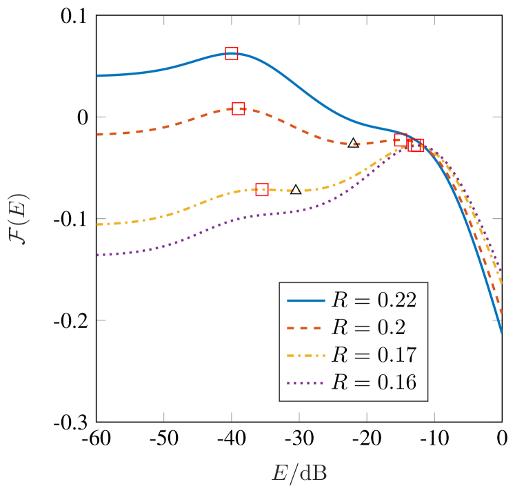
Figure 1: Free energy function at different rates $R$ for $B=1$, $\sigma_{\mathsf{w}}^{2}=-35\operatorname{\mathrm{dB}}$, and sparsity $\epsilon=0.1$. Red squares and black triangles indicate local maxima and minima, respectively.

IV Replica Analysis

In [26], the replica method was used to determine the mse performance of Vbamp for the measurement (1) and the bg prior (3), assuming $\bm{\Sigma}_{\vec{\bm{\mathsf{x}}}}=\mathbf{I}$ and isotropic uncorrelated noise, i.e., $\bm{\Sigma}_{\vec{\bm{\mathsf{w}}}}=\sigma_{\mathsf{w}}^{2}\mathbf{I}$. In this special case mmv and dcs (referred to as MMV-2 and MMV-1, respectively, in [26]) are equivalent. The analysis is quite sophisticated and the generalization to arbitrary signal and noise correlations seems infeasible. However, due to the joint diagonalization approach from Section III, it suffices to extend the replica analysis to the case with $\bm{\Sigma}_{\vec{\bm{\mathsf{x}}}}=\mathbf{I}$ and $\bm{\Sigma}_{\vec{\bm{\mathsf{w}}}}=\operatorname{diag}(\sigma_{\mathsf{w}}^{2}(1),\ldots,\sigma_{\mathsf{w}}^{2}(B))$. In particular, the replica method is capable of predicting the fixed points of Vbamp in the asymptotic regime ($N,M\rightarrow\infty$, $R=M/N=\mathrm{const.}$), as a function of the set of $B$ mse[34, 35]. We note that rigorous equivalence between the replica method and se is not always guaranteed and requires additional technicalities [36]. Assuming $\bm{\Sigma}_{\vec{\bm{\mathsf{x}}}}=\mathbf{I}$ and $\bm{\Sigma}_{\vec{\bm{\mathsf{w}}}}=\operatorname{diag}\big{(}\sigma_{\mathsf{w}}^{2}(1),\ldots,\sigma_{\mathsf{w}}^{2}(B)\big{)}$, we compute in Appendix -C, following the derivation in [26], the free energy $\mathcal{F}(\vec{\mathbf{E}})$ as a function of the mse vector $\vec{\mathbf{E}}=(E(1),\ldots,E(B))^{T}$ with $E(b)=\mathrm{MSE}(b)$, resulting in

$$\begin{split}&\mathcal{F}(\vec{\mathbf{E}})=(1-\epsilon)\,\zeta(\gamma)+\epsilon\,\zeta\Big{(}\frac{\gamma}{1+\gamma}\Big{)}\\ &{}-\frac{R}{2}\sum_{b=1}^{B}\left(\log\frac{2\pi R}{\gamma(b)}+\gamma(b)\sigma_{\mathsf{w}}^{2}(b)-\frac{1-\epsilon}{R}\frac{\gamma(b)}{1+\gamma(b)}\right)\!.\end{split}$$ (17)

In this expression we used

$$\zeta(\eta) =\int\log\left(\epsilon\prod_{b=1}^{B}(1+\gamma(b))^{-\frac{1}{2}}\right.$$

$$\qquad+\left.(1-\epsilon)\exp\!\bigg{(}\!-\frac{1}{2}\sum_{b=1}^{B}\eta(b)\,h^{2}(b)\bigg{)}\right)\mathcal{D}\mathbf{h}$$

with

$$\gamma(b)=\frac{R}{E(b)+R\sigma_{\mathsf{w}}^{2}(b)};$$

furthermore, $\mathcal{D}\mathbf{h}=\mathcal{N}(\mathbf{h};\mathbf{0},\mathbf{I})\,dh_{1}\dots dh_{B}$ denotes the multivariate standard Gaussian measure.

The stationary points of $\mathcal{F}(\vec{\mathbf{E}})$ correspond to fixed points of belief propagation [37], and hence to those of Vbamp in the asymptotic regime [26]. Thus, we can determine the component-wise mses of Vbamp by evaluating (17) and finding the largest components of $\vec{\mathbf{E}}$ that correspond to a local maximum of $\mathcal{F}(\vec{\mathbf{E}})$ [38, 39]. Note that for isotropic noise ($\sigma_{\mathsf{w}}^{2}(b)=\sigma_{\mathsf{w}}^{2}$ $\forall b$), the free energy in (17) simplifies to the result obtained in [26] with one-dimensional argument $E=E(1)=\ldots=E(B)$. Replica curves for the isotropic case with $B=1$ and $B=10$ are shown in Figure 1 and 2 respectively. It is important to point out here that all the plots are the result of numerical integrations (and not Monte Carlo simulations). In the free energy function, local maxima correspond to stable fixed points and local minima to unstable fixed points, whereas the global maximum of $\mathcal{F}(E)$ corresponds to the mmse. Vbamp typically achieves the largest mse associated with a local maximum.

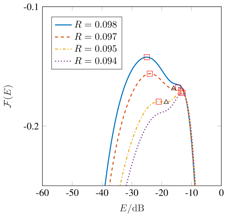
Figure 2: One-dimensional free energy function for the isotropic case with $B=10$ jointly sparse bg vectors at rates around the phase transition rate ($\bm{\Sigma}_{\vec{\bm{\mathsf{w}}}}=-35\operatorname{\mathrm{dB}}\mathbf{I}_{B}$).

IV-A MMSE Gap

In the cs regime of small $\epsilon$ and nonzero noise variance, the mmse estimate $\hat{\mathbf{x}}$ for a single measurement features a first order phase transition (PT) characterized by an abrupt change of the mse at a certain rate $R_{\operatorname{\mathrm{PT}}}$: for rates less than $R_{\operatorname{\mathrm{PT}}}$, the mse tends to be large, whereas for rates larger than $R_{\operatorname{\mathrm{PT}}}$ the mse tends to be small and plateaus to fixed nonzero value. This phenomenon can be seen in Figure 1: for rates below $R\approx 0.16$, where the free energy has a single maximum at an mse of about $-12\operatorname{\mathrm{dB}}$ whereas for rates larger than $R\approx 0.17$ a second local maximum at mse less then about $-37\operatorname{\mathrm{dB}}$ appears.

A similarly abrupt phase transition does not appear to occur when the number of measurements $B$ is sufficiently large. Figure 3 shows the se curves for various $B$ with $\epsilon=0.1$ and $\bm{\Sigma}_{\vec{\bm{\mathsf{x}}}}=\mathbf{I}_{B}$. Observe that the “bump” in the se curve for small $B$ and large mse, which corresponds to the first fixed point, flattens out with increasing $B$. For large enough $B$ we observe that the se curve ceases to exhibit a first order PT, so that the mse changes smoothly with increasing rate $R$.

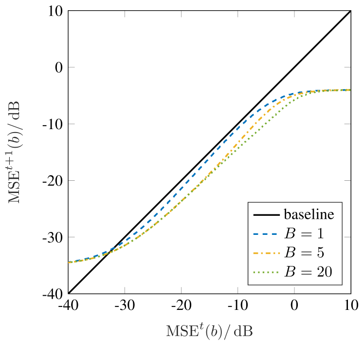
Figure 3: Noisy se curves for different number of jointly sparse bg signals ($\epsilon=0.1$, $\bm{\Sigma}_{\vec{\bm{\mathsf{x}}}}=\mathbf{I}_{B}$, $\bm{\Sigma}_{\vec{\bm{\mathsf{w}}}}=-35\operatorname{\mathrm{dB}}\mathbf{I}_{B}$, $R=0.25$).

The same conclusion can be obtained by investigating the behavior of the free energy functions. Vbamp typically achieves the largest mse which corresponds to a local maximum in the free energy, whereas the mse at the global maximum of the free energy is the mmse. As pointed out in [26], whenever the free energy function has a second local maximum at a larger mse than the global maximum, Vbamp is not Bayesian-optimal (i.e., does not reach the mmse). For $B=1$, in Figure 1, a second local (non-global) maximum appears and thus BAMP is not MMSE optimal in the rate region $0.19<R<0.21$, while for $B=10$ with isotropic noise and sparsity $\epsilon=0.1$ it occurs at $R=0.097$ as shown in Figure 2. We speculate that the vanishing of the first order PT for sufficiently large $B$ may be a typical behaviour and something worthy of further investigation.

While the possibility of no phase transition might appear surprising this relies on the presence of finite measurement noise. In such a setting there is no exact recovery PT. It would be interesting to understand what happens when the noise tends to zero, and see if comparisons could be drawn with PT results for the related problem of block sparse recovery [40], [41]. However, under this scenario it is not clear what would be the role of any anisotropy in the covariance matrices.

Finally, we emphasize that while our analysis here is asymptotic in the large system limit ($N,M,\epsilon N\rightarrow\infty$), it is non-asymptotic in the number of jointly sparse vectors $B$ which are assumed to be $\mathcal{O}(1)$. This is in contrast to existing work [42, 43], where results on the PT like phenomena were derived for the asymptotic case where $B\rightarrow\infty$ as $N\rightarrow\infty$.

V Anisotropic Vbamp Dynamics

We now consider the anisotropic scenaro.

V-A Correlated CS

The matrix $\mathbf{T}$ from Algorithm 2 simultaneously decorrelates the signal and the noise. While $\mathbf{T}\bm{\Sigma}_{\vec{\bm{\mathsf{x}}}}\mathbf{T}^{T}=\mathbf{I}$, the transformed noise covariance $\bm{\Sigma}_{\tilde{\vec{\bm{\mathsf{w}}}}}=\mathbf{T}\bm{\Sigma}_{\vec{\bm{\mathsf{w}}}}\mathbf{T}^{T}$ depends on $\bm{\Sigma}_{\vec{\bm{\mathsf{x}}}}$ and $\bm{\Sigma}_{\vec{\bm{\mathsf{w}}}}$ in a nontrivial way unless $\bm{\Sigma}_{\vec{\bm{\mathsf{x}}}}$ and $\bm{\Sigma}_{\vec{\bm{\mathsf{w}}}}$ commute. In this case, they have identical eigenvectors, i.e., $\bm{\Sigma}_{\vec{\bm{\mathsf{x}}}}=\mathbf{Q}\bm{\Lambda}_{\vec{\mathbf{x}}}\mathbf{Q}^{T}$ and $\bm{\Sigma}_{\vec{\bm{\mathsf{w}}}}=\mathbf{Q}\bm{\Lambda}_{\vec{\mathbf{w}}}\mathbf{Q}^{T}$, and we can show

$$\bm{\Sigma}_{\tilde{\vec{\bm{\mathsf{w}}}}}=\bm{\Lambda}_{\vec{\mathbf{w}}}\bm{\Lambda}_{\vec{\mathbf{x}}}^{-1}=\operatorname{diag}\bigg{(}\frac{\lambda_{\vec{\mathbf{w}}}(1)}{\lambda_{\vec{\mathbf{x}}}(1)},\dots,\frac{\lambda_{\vec{\mathbf{w}}}(B)}{\lambda_{\vec{\mathbf{x}}}(B)}\!\!\bigg{)}.$$

Special cases of this situation occur when (i) either $\bm{\Sigma}_{\vec{\bm{\mathsf{x}}}}$ or $\bm{\Sigma}_{\vec{\bm{\mathsf{w}}}}$ is a scaled identity matrix and (ii) when both $\bm{\Sigma}_{\vec{\bm{\mathsf{x}}}}$ and $\bm{\Sigma}_{\vec{\bm{\mathsf{w}}}}$ are diagonal. The per-channel snr are then obtained from $\bm{\Sigma}_{\tilde{\vec{\bm{\mathsf{w}}}}}$ as $\operatorname{\mathrm{SNR}}(b)=\epsilon\lambda_{\vec{\mathbf{x}}}(b)/\lambda_{\vec{\mathbf{w}}}(b)$. While this result does not hold when $\bm{\Sigma}_{\vec{\bm{\mathsf{x}}}}$ and $\bm{\Sigma}_{\vec{\bm{\mathsf{w}}}}$ do not commute, it is possible to derive the bounds

$$\epsilon\,\frac{\min_{k}\{\lambda_{\vec{\bm{\mathsf{x}}}}(k)\}}{\max_{k}\{\lambda_{\vec{\bm{\mathsf{w}}}}(k)\}}\leq\operatorname{\mathrm{SNR}}(b)\leq\epsilon\,\frac{\max_{k}\{\lambda_{\vec{\bm{\mathsf{x}}}}(k)\}}{\min_{k}\{\lambda_{\vec{\bm{\mathsf{w}}}}(k)\}}.$$

If a subset $\mathbf{x}(b_{1}),\ldots,\mathbf{x}(b_{K})$ of the $B$ signal vectors is fully correlated, then $K-1$ of the snr equal $0$. Thus, the model is equivalent to one with $B-K+1$ (instead of $B$) measurements, but with different snr. The free energy function leads to the same conclusion: when taking the limits $\sigma_{\mathsf{w}}^{2}(b_{1})=\ldots=\sigma_{\mathsf{w}}^{2}(b_{K-1})\rightarrow\infty$ in the $B$-dimensional free energy function (17), it can be seen that $\mathcal{F}(\vec{\mathbf{E}})$ is independent of $E(b_{1}),\ldots,E(b_{K-1})$. Therefore, the curvature of $\mathcal{F}(\vec{\mathbf{E}})$ and hence the location of its stationary points do not depend on those arguments, such that the $B$-dimensional free energy function effectively collapses into a $B-K+1$-dimensional function.

Figure 4 illustates an anisotropic scenario with $B=2$ and the channel noise independent but with different variances: $\sigma_{\mathsf{w}}^{2}(1)=-45\operatorname{\mathrm{dB}}$, and $\sigma_{\mathsf{w}}^{2}(2)=-25\operatorname{\mathrm{dB}}$. In the top row the arrows in the MSE plane depict the se prediction

$$(\operatorname{MSE}^{t}(1),\operatorname{MSE}^{t}(2))\rightarrow(\operatorname{MSE}^{t+1}(1),\operatorname{MSE}^{t+1}(2)).$$

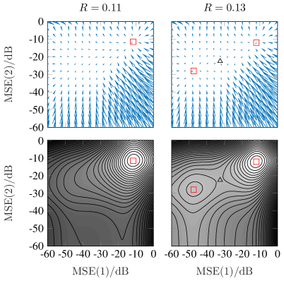
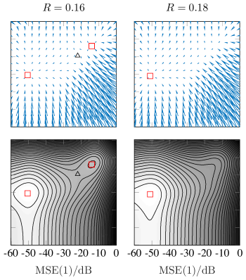
Figure 4: se (top) and free energy (bottom) for $B=2$, $\epsilon=0.1$, $\bm{\Sigma}_{\vec{\bm{\mathsf{x}}}}=\mathbf{I}_{2}$, $\sigma_{\mathsf{w}}^{2}(1)=-45\operatorname{\mathrm{dB}}$, and $\sigma_{\mathsf{w}}^{2}(2)=-25\operatorname{\mathrm{dB}}$. Red squares indicate stable fixed points and local maxima whereas black triangles indicate unstable fixed points and saddle points.

The bottom row shows the free energy function (via gray shading and contour lines). Note that the free energy function is no longer symmetric between channels and both the free energy function and the se dynamics are nontrivially 2-D. However, it is interesting to note that the stationary points still appear to lie on a globally attracting 1-D submanifold. This raises the question of whether the $B$-dimensional se dynamics can be compressed back into a one-dimensional evolution in some way.

There is also a close match between the fixed points of the se and the stationary points of the free energy function, as well as between the se arrows and the gradient of the free energy. This match was confirmed in several other numerical experiments. This opens up the possibility for more detailed investigations with different sets of parameters $\sigma_{\mathsf{w}}^{2}(1),\ldots,\sigma_{\mathsf{w}}^{2}(B)$ to shed light on the performance regions and dynamics of Vbamp. The question arises whether for a given sparsity $\epsilon$ and measurement rate $R$ there is a diversity function $\theta_{\epsilon,R}(\sigma_{\mathsf{w}}^{2}(1),\ldots,\sigma_{\mathsf{w}}^{2}(B))$ that describes the effective number of jointly sparse measurements based on the individual SNR. More specifically, we expect such a diversity function to combine the snr such that, for a certain threshold $B_{0}$, the global maximum of the free energy equals the Vbamp fixed point for $\theta_{\epsilon,R}\geq B_{0}$ while for $\theta_{\epsilon,R}<B_{0}$ the free energy has local maxima to the right of the global maximum, which then is no longer the Vbamp fixed point.

VI Single-Pixel Color Imaging

We applied MMV-BAMP (cf. Algorithm 1) to color imaging using the single-pixel approach from [9]. Here, white light illuminates an object and $M$ random 0/1-masks of dimension $\sqrt{N}\times\sqrt{N}$ with exactly $N/2$ ones are applied before the intensities of the red ($b=1$), green ($b=2$), and blue ($b=3$) components are measured by noisy single-pixel sensors (hence, $B=3$). The $B=3$ discrete cosine transform (DCT) coefficient vectors of the acquired image are assumed to be jointly sparse and drawn from a multivariate bg pdf (with the exception of the DC term as explained below). The measurement matrix is given by $\mathbf{A}=\mathbf{\Phi}\mathbf{D}^{T}$, where the $M\times N$ matrix $\mathbf{\Phi}$ contains the $M$ vectorized binary masks and $\mathbf{D}$ is the DCT matrix. Since $\mathbf{A}$ is the same for all $B=3$ color channels we have an MMV problem. The measurement matrix $\mathbf{A}$ does not satisfy the conditions (zero mean and normalized columns) required for BAMP. Appendix -E explains how to convert this problem into an equivalent form that meets the BAMP requirements.

VI-A Real-world Data

In order to benchmark the recovery algorithms in a real-world setting, we randomly selected a training set of $40$ natural images (see [44, 45]) and a distinct test image (shown in Figure 5). All images had a resolution of $100\times 100$ pixels ($N=10\,000$). The parameters of the BG prior (sparsity $\epsilon$ and covariance matrix $\bm{\Sigma}_{\vec{\bm{\mathsf{x}}}}$) and the parameters of the three scalar bg priors (one for each color channel) were estimated from the training set using the em algorithm [46]. The measurement noise was i.i.d. zero-mean Gaussian with a standard deviation of $\sigma_{\mathsf{w}}(1)=\sigma_{\mathsf{w}}(3)=1.5$ for the red and the blue channels and $\sigma_{\mathsf{w}}(2)=6$ for the green channel. The number of measurements was $M=3330$ ($R=0.333$).

Figure 5 shows the recovery results for (i) AMP with soft thresholding [20], applied independently in each color channel (using the optimal threshold parameter), (ii) scalar bamp, independently applied in each color channel, and (iii) MMV-BAMP (using the estimated bg prior). Figure 5 shows that MMV-BAMP indeed outperforms the scalar schemes. Since the color channels are affected by different noise variance, per-channel AMP and BAMP suffer from a color mismatch. In contrast, MMV-BAMP does not suffer from this problem and yields less blurry edges and clearer image details.

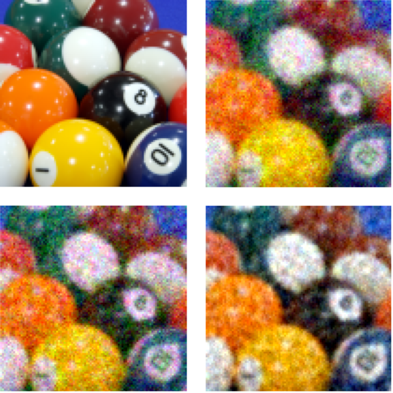
Figure 5: Performance comparison for single-pixel color imaging at $R=0.333$: original image (top left), per-channel AMP with soft-thresholding (top right), per-channe BAMP (bottom left), and MMV-BAMP (bottom right).

Table I: Mean recovery NMSE for AMP, BAMP, MMV-BAMP, and group lasso (the 95%-confidence levels are approximately $\pm 1\operatorname{\mathrm{dB}}$).

	NMSE [dB]
	red	green	blue
AMP	$-16.5$	$-12.7$	$-14.5$
BAMP	$-16.6$	$-12.2$	$-14.7$
MMV-BAMP	$-16.8$	$-14.1$	$-14.9$
group lasso	$-16.4$	$-13.3$	$-14.5$

Table I shows the normalized mean square recovery error (NMSE) achieved by the various methods on the three color channels (the NMSE was estimated by averaging over 40 test images). The table also shows the results obtained with the group lasso [47] based on ADMM [47, 48, 49] with hand-optimized regularization parameter.

MMV-BAMP is seen to outperform all competing schemes. Its performance advantage is most pronounced for the green channel, which has the poorest SNR of $51.9$ dB. For the red and blue channels (SNR $64.8$ and $62.6$ dB, respectively), the performance differences tend to be smaller. We emphasize that MMV-BAMP achieves these performance gains in spite of a mismatched prior, i.e., the distribution of the (jointly sparse) DCT coefficients of natural images is not actually bg.

VI-B Synthetic Data

To eliminate effects resulting from mismatched priors, we next consider artificial images whose red, green, and blue channel DCT coefficients are jointly sparse and have bg distribution. More specifically, we created images having a resolution of $100\times 100$ pixels ($N=10\,000$) by randomly drawing $20\times 20=400$ low-frequency DCT coefficients (on each color channel) from a Gaussian distribution with covariance matrix $(\bm{\Sigma}_{\vec{\bm{\mathsf{x}}}})_{ij}=4-|i\!-\!j|$, $i,j\in\{1,2,3\}$ (except the DC coefficients that had a fixed value of $20$). The remaining $9\,600$ high-frequency DCT coefficients per channel were set to zero. The resulting sparsity equals $\epsilon=400/10\,000=4\%$.

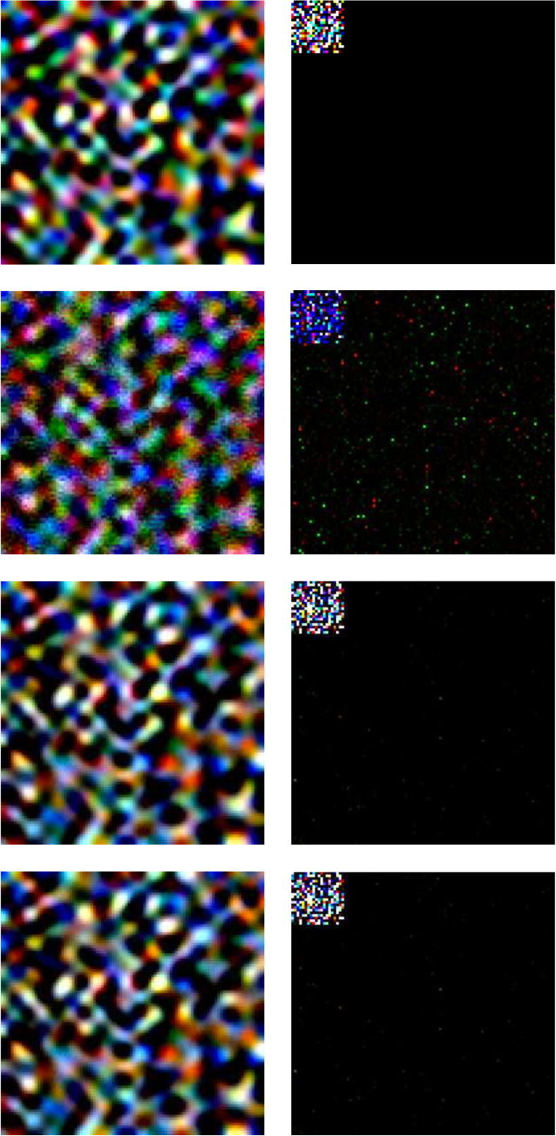
Figure 6: Single-pixel recovery of an artificial image (left column) at $R=0.333$ and corresponding DCT coefficients (right column): original image (top row), BAMP (second row), MMV-BAMP (third row), and MMV-BAMP-EM (bottom row).

We then applied compressive single-pixel imaging as described above to these artificial images. The sampling rate was $R=0.333$ and the standard deviation of the measurement noise in the red and the green channels was eight times larger than that in the blue channel leading to measurement SNRs of $32.4$ dB, $32.4$ dB, and $50.5$ dB, respectively. Recovery was done using BAMP, MMV-BAMP with perfect prior knowledge, and a practical variant labeled MMV-BAMP-EM. The latter augments MMV-BAMP with an on-the-fly (i.e., during the recovery iterations) EM-based estimation of the model parameters (sparsity, mean, and covariance in the bg prior). As shown in [33], this is possible whenever the structure of the prior distribution is known. More specifically, the EM algorithm is applied in Algorithm 1 after line 6 to estimate the parameters of a mixture of two multivariate Gaussians from the decoupled measurements $\mathbf{u}^{t-1}(b)$. The covariance of the stronger of the two mixture components is discounted for the noise and retained for the non-zero part of the bg model.

Figure 6 shows the results for an exemplary artificial image and its DCT. MMV-BAMP is seen to perform much better than BAMP. Furthermore, MMV-BAMP-EM yields recovery results virtually identical to MMV-BAMP. Thus, estimating the prior parameters during recovery induces a negligible performance loss (indeed, we verified that the EM estimates of sparsity and covariance were close to the true values even though based on only $3\times 400$ nonzero DCT coefficients). The DCT domain results also show that the majority of errors occurs in the red and the green channels that suffer from poor SNR.

Table II: Mean recovery NMSE for AMP, BAMP, MMV-BAMP, MMV-BAMP EM, and group lasso (the 95%-confidence levels are less than $\pm 0.1\operatorname{\mathrm{dB}}$).

	NMSE [dB]
	red	green	blue
AMP	$-2.76$	$-2.81$	$-17.53$
BAMP	$-3.92$	$-3.96$	$-23.32$
MMV-BAMP	$-8.36$	$-9.52$	$-23.91$
MMV-BAMP-EM	$-8.34$	$-9.49$	$-23.90$
group lasso (small $\lambda$)	$-0.21$	$-0.30$	$-11.10$
group lasso (moderate $\lambda$)	$-5.00$	$-5.30$	$\;\,-6.80$

A systematic performance comparison in terms of NMSE (obtained by averaging over 100 artificial images) is provided in Table II, which also shows the results achieved by the group lasso. It is seen that MMV-BAMP and MMV-BAMP-EM achieve almost identical NMSE and outperform (B)AMP by exploiting the correlation between the color channels. The performance gain is specifically noticeable in the low-SNR red and green channels, with the gain in the green channel being slightly larger since its correlation with the high-SNR blue channel is stronger ($(\bm{\Sigma}_{\vec{\bm{\mathsf{x}}}})_{23}=3$) than that of the red channel ($(\bm{\Sigma}_{\vec{\bm{\mathsf{x}}}})_{13}=2$).

The group lasso is seen to perform much worse than MMV-BAMP(-EM) since it is unaware of the different measurement SNRs on the three channels. With weak regularization (small $\lambda$), the group lasso relies more on the measurements and hence yields reasonable performance only for the high-SNR blue channel. With stronger regularization (moderate $\lambda$), the group lasso enforces stronger sparsity, which is beneficial for the low-SNR red and green channels but leads to increased distortions on the blue channel. This shows that MMV-BAMP has strong advantages over group lasso when the quality of the measurements of the correlated components is different and unknown.

VII Conclusions

We reviewed the multivariate Vbamp algorithm for mmv/dcs cs recovery and its associated multivariate se. We established that for arbitrary mmv measurement models there is an equivalent model in which signal and noise are both decorrelated. For the widely employed multivariate bg signal prior, we proved that uncorrelatedness is preserved during the Vbamp and se iterations; thus, the complexity of Vbamp for bg signals scales only linearly with the number of jointly sparse vectors. The free energy formula for the jointly sparse bg cs channel with $B$ degrees of freedom has been derived and juxtaposed with the multivariate se. Our results allowed us to assess the impact of signal correlation and of the number of jointly sparse vectors on the phase transition phenomenon and the optimality rate region of Vbamp. Numerical results for single-pixel color imaging demonstrated that MMV-BAMP achieves superior recovery quality by exploiting correlation between the vector components. MMV-BAMP can be augmented with em-based estimation of the parameters of the bg prior, leading to a practical and flexible scheme with excellent recovery performance and significantly smaller complexity than competing approaches such as group lasso.

-A Equivariance of MMV VBAMP and its SE

Consider Algorithm 1 with the transformed variables $\bm{\Sigma}_{\tilde{\vec{\bm{\mathsf{x}}}}}$, $\mathbf{T}\hat{\vec{\mathbf{x}}}_{n}^{t}$, $\mathbf{T}\vec{\mathbf{r}}_{m}^{t}$, $\mathbf{T}\vec{\mathbf{u}}_{n}^{t}$, $\bm{\Sigma}_{\tilde{\vec{\bm{\mathsf{v}}}}}^{t}$. Lines $5$ and $6$ are trivially equivariant. The equivariance of line 7 follows from the invariance property of mmse estimators to affine transformations [50, Ch. 11.4]. In the residual term (line 8), the equivariance of $\vec{\mathbf{y}}_{m}-\big{(}\mathbf{A}(1)\hat{\mathbf{x}}(1)^{t},\ldots,\mathbf{A}(B)\hat{\mathbf{x}}(B)^{t}\big{)}_{m}$ is trivial. It remains to show that the Onsager term is equivariant. Thus, we write the transformed Onsager term as

$$\frac{1}{M}\sum_{n=1}^{N}F^{\prime}(\mathbf{T}\vec{\mathbf{u}}_{n};\mathbf{T}\bm{\Sigma}_{\vec{\bm{\mathsf{v}}}}\mathbf{T}^{T})\mathbf{T}\vec{\mathbf{r}}_{m}$$

$$\stackrel{{\scriptstyle\{1\}}}{{=}}\frac{1}{M}\sum_{n=1}^{N}\operatorname{Cov}\{\tilde{\vec{\mathbf{x}}}\mid\mathbf{T}\vec{\mathbf{u}}_{n};\mathbf{T}\bm{\Sigma}_{\vec{\bm{\mathsf{v}}}}\mathbf{T}^{T}\}\big{(}\mathbf{T}\bm{\Sigma}_{\vec{\bm{\mathsf{v}}}}\mathbf{T}^{T}\big{)}^{-1}\mathbf{T}\vec{\mathbf{r}}_{m}$$

$$=\frac{1}{M}\sum_{n=1}^{N}\operatorname{E}\{\bm{\langle}\tilde{\vec{\mathbf{x}}}-\operatorname{E}\{\tilde{\vec{\mathbf{x}}}\}\bm{\rangle}\mid\mathbf{T}\vec{\mathbf{u}}_{n};\mathbf{T}\bm{\Sigma}_{\vec{\bm{\mathsf{v}}}}\mathbf{T}^{T}\}\mathbf{T}^{-T}\bm{\Sigma}_{\vec{\bm{\mathsf{v}}}}^{-1}\vec{\mathbf{r}}_{m}$$

$$=\frac{1}{M}\sum_{n=1}^{N}\mathbf{T}\operatorname{E}\{\bm{\langle}\vec{\mathbf{x}}-\operatorname{E}\{\vec{\mathbf{x}}\}\bm{\rangle}\mid\vec{\mathbf{u}}_{n};\bm{\Sigma}_{\vec{\bm{\mathsf{v}}}}\}\mathbf{T}^{T}\mathbf{T}^{-T}\bm{\Sigma}_{\vec{\bm{\mathsf{v}}}}^{-1}\vec{\mathbf{r}}_{m}$$

$$\stackrel{{\scriptstyle\{2\}}}{{=}}\mathbf{T}\frac{1}{M}\sum_{n=1}^{N}\operatorname{Cov}\{\vec{\mathbf{x}}\mid\vec{\mathbf{u}}_{n};\bm{\Sigma}_{\vec{\bm{\mathsf{v}}}}\}\bm{\Sigma}_{\vec{\bm{\mathsf{v}}}}^{-1}\vec{\mathbf{r}}_{m}$$

$$=\mathbf{T}\frac{1}{M}\sum_{n=1}^{N}F^{\prime}(\vec{\mathbf{u}}_{n};\bm{\Sigma}_{\vec{\bm{\mathsf{v}}}})\vec{\mathbf{r}}_{m}\,,$$

where $\{1\}$ and $\{2\}$ follow from Lemma 2 in Appendix D. The equivariance of se follows by similar arguments using elementary probability theory and the invariance property of mmse estimators to affine transformations [50, Ch. 11.4].

-B Diagonality of SE with BG Prior

We show that mmv se (11) preserves diagonality for the bg prior. In particular, we prove that if $\bm{\Sigma}_{\vec{\bm{\mathsf{v}}}}^{t}$, $\bm{\Sigma}_{\vec{\bm{\mathsf{w}}}}$ and $\bm{\Sigma}_{\vec{\bm{\mathsf{x}}}}$ are diagonal, then

$$\bm{\Sigma}_{\vec{\bm{\mathsf{v}}}}^{t+1}=\bm{\Sigma}_{\vec{\bm{\mathsf{w}}}}+\frac{1}{R}\underbrace{\operatorname{E}_{\vec{\bm{\mathsf{x}}},\vec{\bm{\mathsf{v}}}}\left\{\bm{\langle}F(\vec{\bm{\mathsf{x}}}+\vec{\bm{\mathsf{v}}}^{t};{\bm{\Sigma}_{\vec{\bm{\mathsf{v}}}}}^{t})-\vec{\bm{\mathsf{x}}}\bm{\rangle}\right\}}_{\mathbf{C}}$$

is also diagonal. It suffices to establish that $\mathbf{C}$ is diagonal. Inserting the bg prior (3) and its estimator (7) and writing out the integrals for $(\mathbf{C})_{i,j}$ ($i,j=1,\ldots,B$), it is seen that for $i\neq j$ the integrands have odd symmetry w.r.t. a separable set of their arguments and thus integrate to $0$. It follows that $(\mathbf{C})_{i,j}=0$ for $i\neq j$ and that $\bm{\Sigma}_{\vec{\bm{\mathsf{v}}}}^{t+1}$ is diagonal.

-C Replica Analysis

Following the analysis in [26], we derive an analytical performance prediction for the Vbamp algorithm for mmv and dcs problems. We consider the measurement model (1) and the signal prior (3) with $\bm{\Sigma}_{\vec{\bm{\mathsf{x}}}}=\mathbf{I}$ and $\vec{\bm{\mathsf{w}}}_{m}\sim\mathcal{N}(\mathbf{0},\bm{\Sigma}_{\vec{\bm{\mathsf{w}}}})$, where $\bm{\Sigma}_{\vec{\bm{\mathsf{w}}}}=\operatorname{diag}(\sigma_{\mathsf{w}}^{2}(1),\ldots\sigma_{\mathsf{w}}^{2}(B))$ is a diagonal matrix with the noise variances $\sigma_{\mathsf{w}}^{2}(b)$. The special case $\bm{\Sigma}_{\vec{\bm{\mathsf{w}}}}=\sigma_{\mathsf{w}}^{2}\mathbf{I}$ was analyzed in [26]. We follow [26] by assuming the rows of $\bm{\mathsf{A}}(b)$ to have variance $\frac{1}{N}$. The straightforward rescaling to normalized columns is discussed at the end. For the sake of notational simplicity, the following derivation applies to the mmv scenario, i.e., $\bm{\mathsf{A}}(1)=\ldots=\bm{\mathsf{A}}(B)=\bm{\mathsf{A}}$. The generalization to dcs is straightforward (cf. [26]). The posterior pdf of the estimate $\hat{\mathbf{X}}=(\hat{\mathbf{x}}(1),\ldots,\hat{\mathbf{x}}(B))=(\hat{\vec{\mathbf{x}}}_{1},\ldots,\hat{\vec{\mathbf{x}}}_{N})^{T}$ reads

$$f_{\hat{\mathbf{X}}\mid\bm{\mathsf{Y}}}(\hat{\mathbf{X}}\mid\mathbf{Y})=\frac{1}{Z}\prod_{n=1}^{N}f_{\hat{\vec{\bm{\mathsf{x}}}}}(\hat{\vec{\mathbf{x}}}_{n})\prod_{m=1}^{M}\mathcal{N}\big{(}(\mathbf{Y}\!-\!\mathbf{A}\hat{\mathbf{X}})_{m};\mathbf{0},\bm{\Sigma}_{\vec{\bm{\mathsf{w}}}}\big{)}$$

with $\mathbf{Y}=(\mathbf{y}(1),\ldots,\mathbf{y}(B))=(\vec{\mathbf{y}}_{1},\ldots,\vec{\mathbf{y}}_{M})^{T}$. Furthermore, $Z$ is the partition function

$$Z=\!\int\displaylimits_{\mathbb{R}^{NB}}\!\prod_{m=1}^{M}\!\mathcal{N}\big{(}(\mathbf{Y}\!-\!\mathbf{A}\hat{\mathbf{X}})_{m};\mathbf{0},\bm{\Sigma}_{\vec{\bm{\mathsf{w}}}}\big{)}\!\prod_{n=1}^{N}\!f_{\hat{\vec{\bm{\mathsf{x}}}}}(\hat{\vec{\mathbf{x}}}_{n})\,d\hat{\vec{\mathbf{x}}}_{n}.$$

Following the argumentation in [26] and the assumptions in [51, 52, 34, 35, 53, 54], we determine the stationary points of the free energy function, which provide the mse in the fixed points of Vbamp along with the mmse for the measurement model (1). The free energy is defined as

$$\mathcal{F}=\lim_{N\rightarrow\infty}\frac{1}{N}\operatorname{E}_{\bm{\mathsf{A}},\bm{\mathsf{X}},\bm{\mathsf{W}}}\left\{\log(Z)\right\},$$ (18)

but in general is difficult to evaluate. The replica method [51, 52, 34, 35, 53, 54] introduces $k$ replicas $\hat{\mathbf{X}}^{1},\ldots,\hat{\mathbf{X}}^{k}$ of the estimate $\hat{\mathbf{X}}$ and approximates the free energy (18) as

$$\mathcal{F}=\lim_{N\rightarrow\infty}\lim_{k\rightarrow 0}\frac{\operatorname{E}_{\bm{\mathsf{A}},\bm{\mathsf{x}},\bm{\mathsf{w}}}\left\{Z^{k}\right\}-1}{Nk}\,.$$ (19)

The self-averaging property that leads to (18) and the replica trick (19) as well as the replica symmetry assumptions are assumed to be valid, even though their theoretical justification is still an open problem [51, 52, 34, 35, 53, 54]. In order to evaluate (18), we write

$$\operatorname{E}_{\bm{\mathsf{A}},\bm{\mathsf{x}},\bm{\mathsf{w}}}\!\left\{Z^{k}\right\}\!=\!\lvert 2\pi\bm{\Sigma}_{\vec{\bm{\mathsf{w}}}}\rvert^{-\frac{k}{2}}\operatorname{E}_{\bm{\mathsf{X}}}\!\bigg{\{}\!\int\!\prod_{m=1}^{M}\!\mathbb{X}_{m}\!\prod_{n=1}^{N}\!\prod_{a=1}^{k}\!f_{\vec{\bm{\mathsf{x}}}}(\vec{\mathbf{x}}_{n}^{a})\,d\vec{\mathbf{x}}_{n}^{a}\!\bigg{\}},$$ (20)

where

$$\mathbb{X}_{m}=\operatorname{E}_{\bm{\mathsf{A}},\bm{\mathsf{W}}}\!\Big{\{}\!\exp\!\Big{(}\!-\frac{1}{2}\|\bar{\vec{\mathbf{v}}}_{m}\|^{2}\!\Big{)}\!\Big{\}}.$$ (21)

Here, we used the vector $\bar{\vec{\mathbf{v}}}_{m}=\bar{\bm{\Sigma}}_{\vec{\bm{\mathsf{w}}}}^{-\frac{1}{2}}\vec{\mathbf{v}}_{m}$ defined in terms of $\vec{\mathbf{v}}_{m}=(v^{1}_{m,1},\ldots,v^{k}_{m,1},v^{1}_{m,2},\ldots,\ldots,v^{k}_{m,B})^{T}$, and $\bar{\bm{\Sigma}}_{\vec{\bm{\mathsf{w}}}}=\bm{\Sigma}_{\vec{\bm{\mathsf{w}}}}\otimes\mathbf{I}_{k\times k}$, where the elements of $\vec{\mathbf{v}}_{m}$ are in terms of

$$\vec{\mathbf{v}}_{m}^{a}=(v_{m,1}^{a},\ldots,v_{m,B}^{a})=\big{(}\mathbf{A}(\mathbf{X}\!-\!\hat{\mathbf{X}}^{a})+\mathbf{W}\big{)}_{m}.$$

Using a Gaussian approximation for the pdf of $\bar{\vec{\mathbf{v}}}_{m}$,

$$f_{\bar{\vec{\bm{\mathsf{v}}}}_{m}}\left(\bar{\vec{\mathbf{v}}}_{m}\right)=\mathcal{N}\left(\bar{\vec{\mathbf{v}}}_{m};\mathbf{0},\mathbf{G}_{m}\right),$$ (22)

(21) can be evaluated as

$$\mathbb{X}_{m}=\lvert\mathbf{I}+\mathbf{G}_{m}\rvert^{-\frac{1}{2}}.$$ (23)

Here, we used the covariance matrix $\mathbf{G}_{m}=\operatorname{Cov}\{\bar{\vec{\mathbf{v}}}_{m}\}=\bar{\bm{\Sigma}}_{\vec{\bm{\mathsf{w}}}}^{-\frac{1}{2}}\bar{\mathbf{G}}_{m}\bar{\bm{\Sigma}}_{\vec{\bm{\mathsf{w}}}}^{-\frac{T}{2}}$ with $\mathbf{G}_{m}=\operatorname{Cov}\{{\vec{\mathbf{v}}}_{m}\}$. The matrix $\bar{\mathbf{G}}_{m}$ is composed of $B\times B$ blocks of size $k\times k$ as follows:

1. The main diagonal of $\bar{\mathbf{G}}_{m}$ consists of entries $g_{1}(b)=\operatorname{E}_{\bm{\mathsf{A}},\bm{\mathsf{w}}}\{(v_{m,b}^{a})^{2}\}$, which is different in each of the $B$ blocks but identical within a block.

2. The remaining entries in the blocks of the main diagonal are $g_{2}(b)=\operatorname{E}_{\bm{\mathsf{A}},\bm{\mathsf{w}}}\{v_{m,b}^{a}v_{m,b}^{a^{\prime}}\}$, which are different in each block but identical within a block.

3. The diagonal entries of the off-diagonal blocks are $g_{3}(b,b^{\prime})=\operatorname{E}_{\bm{\mathsf{A}},\bm{\mathsf{w}}}\{v_{m,b}^{a}v_{m,b^{\prime}}^{a}\}$.

4. The off-diagonal entries of the off-diagonal blocks are $g_{4}(b,b^{\prime})=\operatorname{E}_{\bm{\mathsf{A}},\bm{\mathsf{w}}}\{v_{m,b}^{a}v_{m,b^{\prime}}^{a^{\prime}}\}$.

Using the normalization of the measurement matrix $\mathbf{A}$, the fact that $\vec{\mathbf{x}}_{n}^{a}$ follows the same distribution as $\vec{\mathbf{x}}_{n}$, and the replica symmetry [34, 35], these values turn out to be

$$g_{1}(b) =\frac{1}{N}\sum_{n=1}^{N}(x_{n}(b)-\hat{x}_{n}^{a}(b))^{2}+1,$$

$$g_{2}(b) =\frac{1}{N}\sum_{n=1}^{N}(x_{n}(b)-\hat{x}_{n}^{a}(b))(x_{n}(b)-\hat{x}_{n}^{a^{\prime}}(b))+1,$$

$$g_{3}(b,b^{\prime}) =\frac{1}{N}\sum_{n=1}^{N}(x_{n}(b)-\hat{x}_{n}^{a}(b))(x_{n}(b^{\prime})-\hat{x}_{n}^{a^{\prime}}(b)),$$

$$g_{4}(b,b^{\prime}) =\frac{1}{N}\sum_{n=1}^{N}(x_{n}(b)-\hat{x}_{n}^{a}(b^{\prime}))(x_{n}(b)-\hat{x}_{n}^{a^{\prime}}(b^{\prime})).$$

By introducing the auxiliary quantities

$$m_{a}(b,b^{\prime}) =\frac{1}{N}\sum_{n=1}^{N}\hat{x}_{n}^{a}(b)x_{n}(b^{\prime}),$$

$$Q_{a}(b,b^{\prime}) =\frac{1}{N}\sum_{n=1}^{N}\hat{x}_{n}^{a}(b)\hat{x}^{a}_{n}(b^{\prime}),$$

$$q_{aa^{\prime}}(b,b^{\prime}) =\frac{1}{N}\sum_{n=1}^{N}\hat{x}_{n}^{a}(b)\hat{x}^{a^{\prime}}_{n}(b^{\prime}),$$

$$q_{0}(b,b^{\prime}) =\frac{1}{N}\sum_{n=1}^{N}x_{n}(b)x_{n}(b^{\prime}),$$

the covariance values can be written as

$$g_{1}(b) =\epsilon-2m_{a}(b,b)+Q_{a}(b,b)+1,$$

$$g_{2}(b) =\epsilon-m_{a}(b,b)-m_{a^{\prime}}(b,b)+q_{aa^{\prime}}(b,b)+1,$$

$$g_{3}(b,b^{\prime}) ={q_{0}(b,b^{\prime})-m_{a}(b^{\prime},b)-m_{a^{\prime}}(b,b)+q_{aa^{\prime}}(b,b),}$$

$$g_{4}(b,b^{\prime}) ={q_{0}(b,b)-m_{a}(b^{\prime},b)-m_{a^{\prime}}(b^{\prime},b)+q_{aa^{\prime}}(b^{\prime},b^{\prime})}.$$

In the Bayesian setting the distribution of $\vec{\mathbf{x}}_{n}$ matches the distribution of $\hat{\vec{\mathbf{x}}}_{n}$ and that of the replicas $\hat{\vec{\mathbf{x}}}^{a}_{n}$, thus $g_{3}(b,b^{\prime})=g_{4}(b,b^{\prime})=0$. Furthermore, due to the replica symmetry [34, 35] $m_{a}(b,b)=m_{a^{\prime}}(b,b)=m(b)$, $Q_{a}(b,b)=Q(b)$, and $q_{aa^{\prime}}(b,b)=q(b)$. It follows that the $\mathbf{G}_{m}$ is a structured matrix that, due to its block structure, can be expressed in terms of all-ones matrices, identity matrices, and Kronecker products. Its $kB$ eigenvalues can straightforwardly be determined as

$$\alpha^{b}_{1}=g_{1}(b)+(k\!-\!1)g_{2}(b),\qquad\alpha^{b}_{2}=g_{1}(b)-g_{2}(b),$$

where the $\alpha^{b}_{1}$ have multiplicity 1 and the $\alpha^{b}_{2}$ have multiplicity $k\!-\!1$. We can thus express (23) as

$$\lvert\mathbf{I}+\mathbf{G}_{m}\rvert^{-\frac{1}{2}} =\Bigg{[}\prod_{b=1}^{B}\Big{(}1+k\frac{\epsilon-2m(b)+q(b)+\sigma_{\mathsf{w}}^{2}(b)}{\sigma_{\mathsf{w}}^{2}(b)+Q(b)-q(b)}\Big{)}$$

$$\phantom{=}\prod_{b=1}^{B}\Big{(}1+\frac{1}{\sigma_{\mathsf{w}}^{2}(b)}(Q(b)-q(b))\Big{)}^{k-1}\Bigg{]}^{-\frac{1}{2}}\,.$$

Using the Taylor series approximation

$$\exp\left(-\frac{x}{2}\right)\approx(1+x)^{-\frac{1}{2}},$$

we obtain

$$\lim_{k\rightarrow 0}\mathbb{X}_{m} =\exp\Big{(}-\frac{k}{2}\sum_{b=1}^{B}\frac{\epsilon-2m(b)+q(b)+\sigma_{\mathsf{w}}^{2}(b)}{\sigma_{\mathsf{w}}^{2}(b)+Q(b)-q(b)}$$

$$\phantom{=}-\log(Q(b)-q(b)+\sigma_{\mathsf{w}}^{2}(b))-\log(\sigma_{\mathsf{w}}^{2}(b))\Big{)}\,.$$

Following the derivation in [26, App.], (20) can be written as

$$\operatorname{E}_{\bm{\mathsf{A}},\bm{\mathsf{X}},\bm{\mathsf{W}}}\left\{Z^{k}\right\}=\int\exp\left(kN\Phi(m_{0},\hat{m}_{0},q,\hat{q},Q,\hat{Q})\right)dm_{0}\,d\hat{m}_{0}\,dq\,d\hat{q}\,dQ\,d\hat{Q}\,.$$

Remember that we are only interested in the stationary points of the free energy expression (20). Thus, we set

$$\mathcal{F}=\Phi(\{m(b)^{*},\hat{m}(b)^{*},q(b)^{*},\hat{q}(b)^{*},Q(b)^{*},\hat{Q}(b)^{*}\}_{b=1,\ldots,B})$$

$$=\frac{1}{2}\sum_{b=1}^{B}\left(Q(b)\hat{Q}(b)-2m(b)\hat{m}(b)+q(b)\hat{q}(b)\right)-\frac{R}{2}\log\big{(}\lvert 2\pi\bm{\Sigma}_{\vec{\bm{\mathsf{w}}}}\rvert\big{)}$$

$$-\frac{R}{2}\sum_{b=1}^{B}\Bigg{(}\frac{\epsilon-2m(b)+q(b)+\sigma_{\mathsf{w}}^{2}(b)}{Q(b)-q(b)+\sigma_{\mathsf{w}}^{2}(b)}$$

$$\hskip 42.67912pt+\log\big{(}Q(b)-q(b)+\sigma_{\mathsf{w}}^{2}(b)\big{)}-\log\big{(}\sigma_{\mathsf{w}}^{2}(b)\big{)}\Bigg{)}$$

$$+\int_{\mathbb{R}^{B}}f_{\vec{\mathbf{x}}}(\vec{\mathbf{x}})\int_{\mathbb{R}^{B}}\log\int_{\mathbb{R}^{B}}f_{\hat{\vec{\mathbf{x}}}}(\hat{\vec{\mathbf{x}}})$$

$$\prod_{b=1}^{B}\exp\Big{(}-\frac{1}{2}\hat{q}(b)\,\hat{x}(b)^{2}+\hat{m}(b)\,\hat{x}(b)x(b)+\sqrt{\hat{m}(b)}\,\hat{x}(b)h(b)\Big{)}d\hat{\vec{\mathbf{x}}}\,\mathcal{D}\vec{\mathbf{h}}\,d\vec{\mathbf{x}},$$ (24)

where the superscript $\cdot^{*}$ denotes stationary points. The stationary points are obtained by differentiation as

$$\frac{d\Phi}{dm(b)} =0\,\Rightarrow\,\hat{m}(b)^{*}=\frac{R}{E(b)+\sigma_{\mathsf{w}}^{2}(b)}=\gamma(b),$$

$$\frac{d\Phi}{dq(b)} =0\,\Rightarrow\,\hat{q}(b)^{*}=\frac{R}{E(b)+\sigma_{\mathsf{w}}^{2}(b)}=\gamma(b),$$

$$\frac{d\Phi}{dQ(b)} =0\,\Rightarrow\,\hat{Q}(b)^{*}=0.$$

Here, we used the substitution $E(b)=Q(b)-q(b)$, and the fact that in the Bayesian setting $q(b)^{*}=m(b)^{*}$, and $Q(b)^{*}=\epsilon$. Substituting back into (24) and using $\vec{\mathbf{E}}=(E(1),\ldots,E(B))^{T}$, we obtain

$$\mathcal{F}(\vec{\mathbf{E}},\bm{\Sigma}_{\vec{\bm{\mathsf{w}}}})=$$

$$-\frac{R}{2}\sum_{b=1}^{B}\left(\log\big{(}2\pi(\sigma_{\mathsf{w}}^{2}(b)+E(b))\big{)}+\frac{\epsilon+\sigma_{\mathsf{w}}^{2}(b)}{E(b)+\sigma_{\mathsf{w}}^{2}(b)}\right)$$

$$\phantom{=}+\int_{\mathbb{R}^{B}}f_{\vec{\mathbf{x}}}(\vec{\mathbf{x}})\int_{\mathbb{R}^{B}}\log\Bigg{(}\int_{\mathbb{R}^{B}}f_{\hat{\vec{\mathbf{x}}}}(\hat{\vec{\mathbf{x}}})$$

$$\phantom{=}\prod_{b=1}^{B}\exp\Big{(}-\frac{1}{2}\gamma(b)\,\hat{x}(b)^{2}+\gamma(b)\hat{x}(b)x(b)+\sqrt{\gamma(b)}\hat{x}(b)h(b)\Big{)}d\hat{\vec{\mathbf{x}}}\Bigg{)}\,\mathcal{D}\vec{\mathbf{h}}\,d\vec{\mathbf{x}},$$

where the second integration is over a standard Gaussian measure, i.e., $\mathcal{D}\mathbf{h}=\prod_{b=1}^{B}\mathcal{N}(h_{b};0,1)dh_{b}=\mathcal{N}(\mathbf{h};\mathbf{0},\mathbf{I})\prod_{b=1}^{B}dh_{b}$. Inserting the signal prior (3) results in

$$\mathcal{F}(\vec{\mathbf{E}},\bm{\Sigma}_{\vec{\bm{\mathsf{w}}}})=-\frac{R}{2}\sum_{b=1}^{B}\left(\log\left(2\pi(\sigma_{\mathsf{w}}^{2}(b)+E(b))\right)+\frac{\epsilon+\sigma_{\mathsf{w}}^{2}(b)}{E(b)+\sigma_{\mathsf{w}}^{2}(b)}\right)$$

$$+(1-\epsilon)\int\log\Bigg{(}(1-\epsilon)+$$

$$\epsilon\int\exp\big{(}-\frac{1}{2}\gamma(b)\hat{x}^{2}+\sqrt{\gamma(b)}\hat{x}(b)h(b)\big{)}\mathcal{D}\mathbf{x}\Bigg{)}\mathcal{D}\vec{\mathbf{h}}$$

$$+\epsilon\int\int\log\Bigg{(}(1-\epsilon)+$$

$$\epsilon\int\exp\big{(}-\frac{1}{2}\gamma(b)\hat{x}(b)^{2}+\gamma(b)\hat{x}(b)x(b)+\sqrt{\gamma(b)}\hat{x}(b)h(b)\big{)}\mathcal{D}\hat{\vec{\mathbf{x}}}\Bigg{)}\mathcal{D}\vec{\mathbf{h}}\,\mathcal{D}\vec{\mathbf{x}}\,,$$

with the measures $\mathcal{D}\vec{\mathbf{x}}$ and $\mathcal{D}\hat{\vec{\mathbf{x}}}$ analogously as above. Further simplification leads to

$$\mathcal{F}(\vec{\mathbf{E}},\bm{\Sigma}_{\vec{\bm{\mathsf{w}}}})$$

$$=-\frac{R}{2}\sum_{b=1}^{B}\left(\log\left(2\pi(\sigma_{\mathsf{w}}^{2}(b)+E(b))\right)+\frac{\epsilon+\sigma_{\mathsf{w}}^{2}(b)}{E(b)+\sigma_{\mathsf{w}}^{2}(b)}-\frac{\gamma(b)(1+\epsilon\gamma(b))}{R(1+\gamma(b))}\right)$$

$$+(1-\epsilon)\!\int\!\log\left(\epsilon\prod_{b=1}^{B}(1+\gamma(b))^{-\frac{1}{2}}\!+\!(1-\epsilon)\exp\big{(}\!-\!\frac{1}{2}\sum_{b=1}^{B}\gamma(b)h^{2}(b)\big{)}\!\right)\!\mathcal{D}\vec{\mathbf{h}}$$

$$+\epsilon\!\int\!\log\left(\epsilon\prod_{b=1}^{B}(1+\gamma(b))^{-\frac{1}{2}}\!+\!(1-\epsilon)\exp\big{(}\!-\!\frac{1}{2}\sum_{b=1}^{B}\frac{\gamma(b)}{1+\gamma(b)}h^{2}(b)\big{)}\!\right)\!\mathcal{D}\vec{\mathbf{h}}.$$

In order to arrive at (17) that is valid for measurement matrices with normalized columns we use the equivalence between the measurement models with normalized rows and normalized columns and replace $\sigma_{\mathsf{w}}^{2}(b)$ with $R\sigma_{\mathsf{w}}^{2}(b)$:

$$\mathbf{y}=\mathbf{A}\mathbf{x}+\mathbf{w}\quad\Longrightarrow\quad\bar{\mathbf{y}}=\frac{1}{\sqrt{R}}\mathbf{y} =\bar{\mathbf{A}}\mathbf{x}+\bar{\mathbf{w}},$$

where $\bar{\mathbf{A}}$ has normalized columns and $\bar{\mathsf{w}}_{m}\sim\mathcal{N}(0,\frac{\sigma_{\mathsf{w}}^{2}}{R})$ if $\mathsf{w}_{m}\sim\mathcal{N}(0,\sigma_{\mathsf{w}}^{2})$.

-D Estimator Derivative and Conditional Correlation

Lemma 2

Given a realization $\mathbf{x}$ of a random vector $\bm{\mathsf{x}}\in\mathbb{R}^{N}$ with pdf $f_{\bm{\mathsf{x}}}(\mathbf{x})$ and its noisy observation

$$\mathbf{u}=\mathbf{x}+\mathbf{w}$$

with $\bm{\mathsf{w}}\sim\mathcal{N}(0,\bm{\Sigma}_{\vec{\bm{\mathsf{w}}}})$ being independent additive Gaussian noise, its mmse estimator is

$$\hat{\mathbf{x}}(\mathbf{u})=\operatorname{E}\left\{\bm{\mathsf{x}}\mid\bm{\mathsf{u}}=\mathbf{u}\right\}\,.$$

Then, the following relation holds:

$$\operatorname{Cov}\left\{\bm{\mathsf{x}}\mid\bm{\mathsf{u}}=\mathbf{u}\right\}=\frac{d}{d\mathbf{u}^{T}}\hat{\mathbf{x}}(\mathbf{u})\bm{\Sigma}_{\vec{\bm{\mathsf{w}}}}\,.$$

Proof 1

Given the definition of the conditional mean and covariance,

$$\operatorname{E}\left\{\bm{\mathsf{x}}\mid\mathbf{u},\bm{\Sigma}_{\vec{\bm{\mathsf{w}}}}\right\} =\frac{1}{f_{\bm{\mathsf{u}}}(\mathbf{u})}\int_{\mathbb{R}^{N}}\mathbf{x}f_{\bm{\mathsf{u}}\mid\bm{\mathsf{x}}}(\mathbf{u}\mid\mathbf{x})f_{\bm{\mathsf{x}}}(\mathbf{x})d\mathbf{x}$$

$$\operatorname{Cov}\left\{\bm{\mathsf{x}}\mid\mathbf{u},\bm{\Sigma}_{\vec{\bm{\mathsf{w}}}}\right\} =\frac{1}{f_{\bm{\mathsf{u}}}(\mathbf{u})}\int_{\mathbb{R}^{N}}\mathbf{x}\mathbf{x}^{T}f_{\bm{\mathsf{u}}\mid\bm{\mathsf{x}}}(\mathbf{u}\mid\mathbf{x})f_{\bm{\mathsf{x}}}(\mathbf{x})d\mathbf{x}$$

$$\phantom{=}-\operatorname{E}\left\{\bm{\mathsf{x}}\mid\mathbf{u}\right\}\operatorname{E}\left\{\bm{\mathsf{x}}\mid\mathbf{u}\right\}^{T}\,,$$

we have

$$\frac{d}{d\mathbf{u}}\hat{\mathbf{x}}(\mathbf{u})\bm{\Sigma}_{\vec{\bm{\mathsf{w}}}}= \frac{1}{f_{\bm{\mathsf{u}}}(\mathbf{u})}\int_{\mathbb{R}^{N}}\mathbf{x}f_{\bm{\mathsf{x}}}(\mathbf{x})\frac{d}{d\mathbf{u}^{T}}f_{\bm{\mathsf{u}}\mid\bm{\mathsf{x}}}(\mathbf{u}\mid\mathbf{x})d\mathbf{x}\,\bm{\Sigma}_{\vec{\bm{\mathsf{w}}}}$$

$$-\int_{\mathbb{R}^{N}}\frac{1}{f_{\bm{\mathsf{u}}}(\mathbf{u})}\mathbf{x}f_{\bm{\mathsf{u}}\mid\bm{\mathsf{x}}}(\mathbf{u}\mid\mathbf{x})f_{\bm{\mathsf{x}}}(\mathbf{x})d\mathbf{x}\,\,\frac{1}{f_{\bm{\mathsf{u}}}(\mathbf{u})}\frac{d}{d\mathbf{u}^{T}}f_{\bm{\mathsf{u}}}(\mathbf{u})\,\bm{\Sigma}_{\vec{\bm{\mathsf{w}}}}\,.$$ (25)

Since $f_{\bm{\mathsf{u}}\mid\bm{\mathsf{x}}}(\mathbf{u}\mid\mathbf{x})=\mathcal{N}(\mathbf{0},\bm{\Sigma}_{\vec{\bm{\mathsf{w}}}})$ [55],

$$\frac{d}{d\mathbf{u}^{T}}f_{\bm{\mathsf{u}}\mid\bm{\mathsf{x}}}(\mathbf{u}\mid\mathbf{x})=f_{\bm{\mathsf{u}}\mid\bm{\mathsf{x}}}(\mathbf{u}\mid\mathbf{x})(\mathbf{x}-\mathbf{u})^{T}\bm{\Sigma}_{\vec{\bm{\mathsf{w}}}}^{-1}\,.$$ (26)

Furthermore, the mmse estimator can be written as [56, 57]

$$\hat{\mathbf{x}}(\mathbf{u})=\mathbf{u}+\bm{\Sigma}_{\vec{\bm{\mathsf{w}}}}\frac{1}{f_{\bm{\mathsf{u}}}(\mathbf{u})}\frac{d}{d\mathbf{u}}f_{\bm{\mathsf{u}}}(\mathbf{u})\,.$$ (27)

Combining (25), (26), and (27) we have

$$\frac{d}{d\mathbf{u}}\hat{\mathbf{x}}(\mathbf{u})\bm{\Sigma}_{\vec{\bm{\mathsf{w}}}}=\frac{1}{f_{\bm{\mathsf{u}}}(\mathbf{u})}\int_{\mathbb{R}^{N}}\mathbf{x}f_{\bm{\mathsf{u}}\mid\bm{\mathsf{x}}}(\mathbf{x}\mid\mathbf{u})(\mathbf{x}-\mathbf{u})^{T}f_{\bm{\mathsf{x}}}(\mathbf{x})d\mathbf{x}$$

$$\phantom{=}-(\hat{\mathbf{x}}(\mathbf{u})-\mathbf{u})\frac{1}{f_{\bm{\mathsf{u}}}(\mathbf{u})}\int_{\mathbb{R}^{N}}\mathbf{x}f_{\bm{\mathsf{u}}\mid\bm{\mathsf{x}}}(\mathbf{u}\mid\mathbf{x})f_{\mathbf{x}}(\mathbf{x})d\mathbf{x}$$

$$=\frac{1}{f_{\bm{\mathsf{u}}}(\mathbf{u})}\int_{\mathbb{R}^{N}}\mathbf{x}\mathbf{x}^{T}f_{\bm{\mathsf{u}}\mid\bm{\mathsf{x}}}(\mathbf{u}\mid\mathbf{x})f_{\bm{\mathsf{x}}}(\mathbf{x})d\mathbf{x}-\hat{\mathbf{x}}(\mathbf{u})\hat{\mathbf{x}}(\mathbf{u})^{T}$$

$$=\operatorname{Cov}\left\{\bm{\mathsf{x}}\mid\mathbf{u}\right\}\,,$$

which completes the proof.

-E Measurement Conversion for Single-Pixel Imaging

We start from the measurement equation (1), where $\mathbf{A}(b)=\mathbf{A}=\mathbf{\Phi}\mathbf{D}^{T}$, $b=1,2,3$. Hence,

$$\mathbf{y}(b)=\mathbf{\Phi}\mathbf{D}^{T}\mathbf{x}(b)+\mathbf{w}(b)\>,$$

where $\mathbf{x}(b)$, $b=1,2,3$, are the vectorized DCT coefficients of the red, green, and blue channels, respectively. The $M\times N$ matrix $\mathbf{\Phi}$ consists of the $M$ vectorized $0/1$ masks $\bm{\phi}_{i}^{T}$ of dimension $1\times N$, each having exactly $N/2$ ones. Furthermore, $\mathbf{D}$ is an $N\times N$ (combined row-column) DCT matrix.

Since all rows of $\mathbf{\Phi}$ have exactly $N/2$ ones and all elements of the first column of $\mathbf{D}^{T}$ equal $1/\sqrt{N}$, it follows that all elements of the first column $\mathbf{a}_{1}$ of $\mathbf{A}$ are equal to ${\sqrt{N}}/{2}$ and hence $\mathbf{a}_{1}$ has mean $\sqrt{N}/2$ and Euclidean norm $\sqrt{MN}/2$. Since the remaining columns $\mathbf{a}_{2},...,\mathbf{a}_{N}$ of $\mathbf{A}$ equal the sum of randomly sampled cosine sequences, their mean is approximately zero and their norm approximately equals $\lVert\mathbf{a}_{i}\rVert_{2}\approx{\sqrt{M}}/{2}$. Since BAMP requires a measurement matrix with zero-mean and unit-norm columns, we compensate for the first column and renormalize the remaining columns, i.e.,

$$\underbrace{\frac{\mathbf{y}(b)-\mathbf{a}_{1}\sqrt{N}x_{1}(b)}{\sqrt{M}/2}}_{\displaystyle\mathbf{\tilde{y}}(b)}=\underbrace{\frac{\Big{(}\mathbf{a}_{2},\mathbf{a}_{3},...,\mathbf{a}_{N}\Big{)}}{\sqrt{M}/2}}_{\displaystyle\mathbf{\tilde{A}}}\begin{pmatrix}x_{2}(b)\\ x_{3}(b)\\ ...\\ x_{N}(b)\end{pmatrix}+\frac{\mathbf{w}(b)}{\sqrt{M}/2}.$$

The new measurement matrix $\mathbf{\tilde{A}}$ now satisfies the BAMP requirements. It remains to find the DC coefficients $x_{1}(b)$, $b=1,2,3$. Denoting the color component vectors by $\bar{\mathbf{x}}(b)=\mathbf{D}^{T}\mathbf{x}(b)$, we have $x_{1}(b)=\sum_{n=1}^{N}\bar{x}_{n}(b)/\sqrt{N}$. Furthermore, since half of the elements of the masks $\bm{\phi}_{i}^{T}$ equal 1 we have $\sum_{i=1}^{M}\bm{\phi}_{i}^{T}\approx\mathbf{1}M/2$ and hence

$$\frac{1}{M}\!\sum_{i=1}^{M}y_{i}(b)=\frac{1}{M}\!\sum_{i=1}^{M}\bm{\phi}_{i}^{T}\bar{\mathbf{x}}(b)+\!\underbrace{\frac{1}{M}\!\sum_{i=1}^{M}w_{i}(b)}_{\approx 0}\approx\frac{1}{2}\!\sum_{n=1}^{N}\bar{x}_{n}(b),$$

thus finally leading to the estimate

$$x_{1}(b)\approx\frac{2}{M\sqrt{N}}\sum_{i=1}^{M}y_{i}(b).$$

References

- [1] D. L. Donoho, “Compressed Sensing,” IEEE Transactions on Information Theory, vol. 52, no. 4, pp. 1289–1306, 2006.
- [2] E. J. Candés, J. K. Romberg, and T. Tao, “Stable signal recovery from incomplete and inaccurate measurements,” Communications on Pure and Applied Mathematics, vol. 59, no. 8, pp. 1207–1223, 2006.
- [3] S. Cotter, B. Rao, K. Engan, and K. Kreutz-Delgado, “Sparse solutions to linear inverse problems with multiple measurement vectors,” IEEE Transactions on Signal Processing, vol. 53, pp. 2477–2488, Jul. 2005.
- [4] M. F. Duarte, S. Sarvotham, M. B. Wakin, D. Baron, and R. G. Baraniuk, “Joint sparsity models for distributed compressed sensing,” in Proceedings of the Workshop on Signal Processing with Adaptative Sparse Structured Representations, IEEE, 2005.
- [5] M. Mayer, G. Hannak, and N. Goertz, “Exploiting joint sparsity in compressed sensing-based RFID,” EURASIP Journal on Embedded Systems, vol. 2016, no. 1, pp. 1–15, 2016.
- [6] D. Liang, L. Ying, and F. Liang, “Parallel MRI Acceleration Using M-FOCUSS,” in 3rd International Conference on Bioinformatics and Biomedical Engineering (ICBBE), pp. 1–4, IEEE, 2009.
- [7] T. Wimalajeewa and P. K. Varshney, “OMP based joint sparsity pattern recovery under communication constraints,” IEEE Transactions on Signal Processing, vol. 62, no. 19, pp. 5059–5072, 2014.
- [8] G. Tzagkarakis, D. Milioris, and P. Tsak, “Multiple-measurement Bayesian compressed sensing using GSM priors for DOA estimation,” in IEEE International Conference on Acoustics Speech and Signal Processing (ICASSP), pp. 2610–2613, 2010.
- [9] M. F. Duarte, M. A. Davenport, D. Takhar, J. N. Laska, T. Sun, K. F. Kelly, and R. G. Baraniuk, “Single-pixel imaging via compressive sampling,” IEEE Signal Processing Magazine, vol. 25, pp. 83–91, 2008.
- [10] J. A. Tropp, A. C. Gilbert, and M. J. Strauss, “Algorithms for simultaneous sparse approximation. Part I: Greedy pursuit,” Signal Processing, vol. 86, no. 3, pp. 572–588, 2006.
- [11] J. A. Tropp, “Algorithms for simultaneous sparse approximation. Part II: Convex relaxation,” Signal Processing, vol. 86, no. 3, pp. 589–602, 2006.
- [12] D. P. Wipf and B. D. Rao, “An empirical Bayesian strategy for solving the simultaneous sparse approximation problem,” IEEE Transactions on Signal Processing, vol. 55, no. 7, pp. 3704–3716, 2007.
- [13] M. E. Davies and Y. C. Eldar, “Rank awareness in joint sparse recovery,” IEEE Transactions on Information Theory, vol. 58, no. 2, pp. 1135–1146, 2012.
- [14] P. Schniter, “Turbo reconstruction of structured sparse signals,” in 2010 44th Annual Conference on Information Sciences and Systems (CISS), pp. 1–6, Mar. 2010.
- [15] J. Ziniel and P. Schniter, “Efficient high-dimensional inference in the multiple measurement vector problem,” IEEE Transactions on Signal Processing, vol. 61, pp. 340–354, Jan. 2013.
- [16] M. Mayer and N. Goertz, “Bayesian optimal approximate message passing to recover structured sparse signals,” ArXiv e-prints, Aug. 2015.
- [17] X. Zhao and W. Dai, “On joint recovery of sparse signals with common supports,” in International Symposium on Information Theory (ISIT), pp. 541–545, IEEE, 2015.
- [18] Y. Lu and W. Dai, “Independent versus repeated measurements: A performance quantification via state evolution,” in International Conference on Acoustics, Speech and Signal Processing (ICASSP), pp. 4653–4657, IEEE, 2016.
- [19] J. Kim, W. Chang, B. Jung, D. Baron, and J. C. Ye, “Belief propagation for joint sparse recovery,” arXiv preprint arXiv:1102.3289, 2011.
- [20] D. L. Donoho, A. Maleki, and A. Montanari, “Message-passing algorithms for compressed sensing,” Proceedings of the National Academy of Sciences, vol. 106, no. 45, pp. 18914–18919, 2009.
- [21] D. Donoho, A. Maleki, and A. Montanari, “Message passing algorithms for compressed sensing: I. Motivation and construction,” in 2010 IEEE Information Theory Workshop on Information Theory (ITW 2010, Cairo), pp. 1–5, Jan. 2010.
- [22] D. Donoho, A. Maleki, and A. Montanari, “Message passing algorithms for compressed sensing: II. Analysis and validation,” in 2010 IEEE Information Theory Workshop on Information Theory (ITW 2010, Cairo), pp. 1–5, Jan. 2010.
- [23] A. Maleki, “Approximate message passing algorithms for compressed sensing.” http://www.ece.rice.edu/mam15/thesis.pdf, PhD Thesis, Department of Electrical Engineering, Stanford University, 2011.
- [24] A. Montanari, “Graphical Models Concepts in Compressed Sensing,” Compressed Sensing: Theory and Applications, pp. 394–438, 2012.
- [25] S. Rangan, A. K. Fletcher, V. K. Goyal, E. Byrne, and P. Schniter, “Hybrid approximate message passing,” IEEE Transactions on Signal Processing, vol. 65, no. 17, pp. 4577–4592, 2017.
- [26] J. Zhu, D. Baron, and F. Krzakala, “Performance limits for noisy multi-measurement vector problems,” IEEE Transactions on Signal Processing, vol. 65, no. 9, pp. 2444–2454, 2017.
- [27] M. Bayati and A. Montanari, “The dynamics of message passing on dense graphs, with applications to compressed sensing,” IEEE Transactions on Information Theory, vol. 57, pp. 764–785, Feb 2011.
- [28] R. Berthier, A. Montanari, and P. M. Nguyen, “State evolution for approximate message passing with non-separable functions,” arXiv preprint arXiv:1708.03950, 2017.
- [29] Y. Ma, C. Rush, and D. Baron, “Analysis of approximate message passing with a class of non-separable denoisers,” in Information Theory (ISIT), 2017 IEEE International Symposium on, pp. 231–235, IEEE, 2017.
- [30] S. Rangan, P. Schniter, and A. K. Fletcher, “Vector approximate message passing,” in Information Theory (ISIT), 2017 IEEE International Symposium on, pp. 1588–1592, IEEE, 2017.
- [31] S. Foucart and H. Rauhut, A mathematical introduction to compressive sensing, vol. 1. Birkhäuser Basel, 2013.
- [32] R. A. Horn and C. R. Johnson, Matrix analysis. Cambridge university press, 2012.
- [33] J. Vila and P. Schniter, “Expectation-maximization Gaussian-mixture approximate message passing,” IEEE Transactions on Signal Processing, vol. 61, pp. 4658–4672, Oct. 2013.
- [34] F. Krzakala, M. Mézard, F. Sausset, Y. Sun, and L. Zdeborová, “Probabilistic reconstruction in compressed sensing: algorithms, phase diagrams, and threshold achieving matrices,” Journal of Statistical Mechanics: Theory and Experiment, vol. 2012, no. 08, p. P08009, 2012.
- [35] F. Krzakala, M. Mézard, F. Sausset, Y. Sun, and L. Zdeborová, “Statistical-physics-based reconstruction in compressed sensing,” Physical Review X, vol. 2, no. 2, p. 021005, 2012.
- [36] G. Reeves and H. D. Pfister, “The replica-symmetric prediction for compressed sensing with Gaussian matrices is exact,” in 2016 IEEE International Symposium on Information Theory (ISIT), pp. 665–669, IEEE, 2016.
- [37] T. Heskes, “Stable fixed points of loopy belief propagation are minima of the Bethe free energy,” Advances in neural information processing systems, vol. 15, pp. 359–366, 2003.
- [38] J. S. Yedidia, W. T. Freeman, and Y. Weiss, “Constructing free-energy approximations and generalized belief propagation algorithms,” IEEE Transactions on Information Theory, vol. 51, no. 7, pp. 2282–2312, 2005.
- [39] J. S. Yedidia, W. T. Freeman, and Y. Weiss, “Bethe free energy, Kikuchi approximations, and belief propagation algorithms,” Advances in neural information processing systems, vol. 13, 2001.
- [40] A. Taeb, A. Maleki, C. Studer, and R. Baraniuk, “Maximin analysis of message passing algorithms for recovering block sparse signals,” arXiv preprint arXiv:1303.2389, 2013.
- [41] D. L. Donoho, I. Johnstone, and A. Montanari, “Accurate prediction of phase transitions in compressed sensing via a connection to minimax denoising,” IEEE transactions on Information Theory, vol. 59, no. 6, pp. 3396–3433, 2013.
- [42] J. D. Blanchard and M. E. Davies, “Recovery guarantees for rank aware pursuits,” IEEE Signal Processing Letters, vol. 19, no. 7, pp. 427–430, 2012.
- [43] J. M. Kim, O. K. Lee, and J. C. Ye, “Compressive MUSIC: revisiting the link between compressive sensing and array signal processing,” IEEE Transactions on Information Theory, vol. 58, no. 1, pp. 278–301, 2012.
- [44] N. Asuni and A. Giachetti, “TESTIMAGES: a large-scale archive for testing visual devices and basic image processing algorithms,” in STAG – Smart Tools & Apps for Graphics Conference, 2014.
- [45] N. Asuni and A. Giachetti, “TESTIMAGES: a large data archive for display and algorithm testing,” Journal of Graphics Tools, vol. 17, no. 4, pp. 113–125, 2015.
- [46] C. M. Bishop, Pattern Recognition and Machine Learning. Springer New York, 2006.
- [47] S. Boyd, N. Parikh, E. Chu, B. Peleato, and J. Eckstein, “Distributed optimization and statistical learning via the alternating direction method of multipliers,” Found. Trends Mach. Learn., vol. 3, pp. 1–122, Jan. 2011.
- [48] S. Boyd, N. Parikh, E. Chu, B. Peleato, and J. Eckstein, “Sum-of-norms regularization (group lasso) with feature splitting / code..” https://web.stanford.edu/~boyd/papers/admm/group_lasso/group_lasso.html, 2011. [Online; accessed 2018-04-11].
- [49] S. Boyd, N. Parikh, E. Chu, B. Peleato, and J. Eckstein, “Sum-of-norms regularization (group lasso) with feature splitting / examples.” https://web.stanford.edu/~boyd/papers/admm/group_lasso/group_lasso_example.html, 2011. [Online; accessed 2018-04-11].
- [50] S. M. Kay, Fundamentals of Statistical Signal Processing, Volume I: Estimation Theory. Prentice Hall, 1993.
- [51] T. Tanaka, “A statistical-mechanics approach to large-system analysis of CDMA multiuser detectors,” IEEE Transactions on Information Theory, vol. 48, no. 11, pp. 2888–2910, 2002.
- [52] D. Guo and S. Verdú, “Randomly spread CDMA: asymptotics via statistical physics,” IEEE Transactions on Information Theory, vol. 51, no. 6, pp. 1983–2010, 2005.
- [53] M. Mezard and A. Montanari, Information, Physics, and Computation. Oxford University Press, 2009.
- [54] J. Barbier and F. Krzakala, “Approximate message-passing decoder and capacity achieving sparse superposition codes,” IEEE Transactions on Information Theory, vol. 63, no. 8, pp. 4894–4927, 2017.
- [55] K. B. Petersen and M. S. Pedersen, “The matrix cookbook,” Technical University of Denmark, vol. 7, p. 15, 2008.
- [56] M. Raphan and E. P. Simoncelli, “Empirical Bayes least squares estimation without an explicit prior,” NYU Courant Inst. Tech. Report, 2007.
- [57] M. Raphan and E. P. Simoncelli, “Least squares estimation without priors or supervision,” Neural computation, vol. 23, no. 2, pp. 374–420, 2011.