CLS 2+1 flavor simulations at physical light- and strange-quark masses

Abstract

We report recent efforts by CLS to generate an ensemble with physical light- and strange-quark masses in a lattice volume of $192\times 96^{3}$ at $\beta=3.55$ corresponding to a lattice spacing of $0.064$ fm. This ensemble is being generated as part of the CLS 2+1 flavor effort with improved Wilson fermions. Our simulations currently cover 5 lattice spacings ranging from $0.039$ fm to $0.086$ fm at various pion masses along chiral trajectories with either the sum of the quark masses kept fixed, or with the strange-quark mass at the physical value. The current status of simulations is briefly reviewed, including a short discussion of measured autocorrelation times and of the main features of the simulations. We then proceed to discuss the thermalization strategy employed for the generation of the physical quark-mass ensemble and present first results for some simple observables. Challenges encountered in the simulation are highlighted.

1 Introduction

The CLS (Coordinated Lattice Simulations) consortium with members in Denmark, Germany, Italy, Spain, and Switzerland has embarked on a program to generate 2+1 flavor gauge ensembles with $O(a)$ improved Wilson fermions and a Lüscher-Weisz gauge action with tree-level coefficients. A special feature is the use of open boundary conditions in the time direction (to avoid topological freezing at fine lattice spacings Luscher:2011kk ) for the bulk of ensembles generated to date. Another feature is the introduction of a small twisted-mass term for the light (up and down) quarks in the simulation together with subsequent reweighting to zero twisted mass (twisted mass reweighting) Luscher:2012av , to avoid accidental near-zero modes of the lattice Dirac operator. Most of the ensembles generated initially Bruno:2014jqa are along a trajectory keeping the trace of the bare quark-mass matrix fixed, $\operatorname{Tr}(M)=\mathrm{const}$. More recently, these ensembles have been supplemented by ensembles along a trajectory with fixed strange quark mass $m_{s}\approx m_{s,phys}$ Bali:2016umi and with $m_{s}=m_{l}$ at different values of $\operatorname{Tr}(M)$.

For the simulation, the highly flexible openQCD package OpenQCD is used. Among its main features are the use of nested hierarchical integrators (for the implementation see Luscher:2012av ), Hasenbusch-style frequency splitting Hasenbusch:2001ne with an arbitrary number of pseudofermion pairs, RHMC Kennedy:1998cu (plus reweighting) for the strange quark, deflation acceleration along the HMC trajectory Luscher:2007se ; Luscher:2007es and a chronological inverter Brower:1995vx . The package implements a number of solvers.

Figure 1: Landscape of CLS 2+1-flavor ensembles with $\operatorname{Tr}(M)=\mathrm{const}$ (left pane) and $m_{s}=\mathrm{const}$ (right pane). In both cases the lattice spacing squared is displayed on the x-axis, while the y axis shows the pion mass. Ensembles still in production are shown in yellow, while ensembles considered complete are shown in green. The physical light-quark mass ensemble E250 discussed in these proceedings is shown in both plots. Multiple ensemble names next to a single dot indicate ensembles with different volumes at the (otherwise) same set of simulation parameters.

Figure 2: Landscape of CLS 2+1-flavor ensembles with $\operatorname{Tr}(M)=\mathrm{const}$ (left pane) and $m_{s}=\mathrm{const}$ (right pane). The area of the circles in this plot is proportional to the number of MDU divided by the largest integrated autocorrelation time $\tau_{int}$

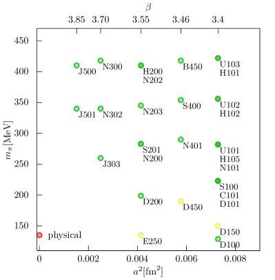
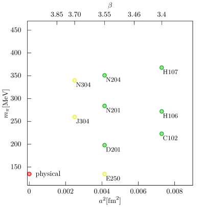
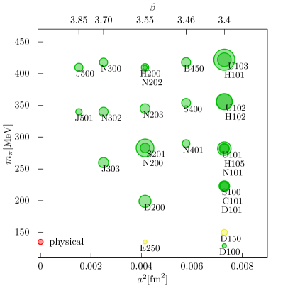
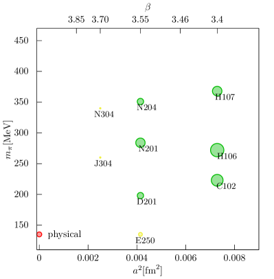
Figure 1 shows the current set of ensembles for both $\operatorname{Tr}(M)=\mathrm{const}$ (left pane) and $m_{s}=\mathrm{const}$ (right pane). The ensembles are labeled by a letter (denoting the aspect ratio $T/L$) and three numerical digits (the first digit encodes $\beta$ and therefore the lattice spacing). Our current library features ensembles at 5 lattice spacings (ranging from $0.039$ fm to $0.086$ fm) and with a range of pion masses $M_{\pi}\leq 420$ MeV. For some sets of parameters, multiple lattice volumes exist, enabling us to control finite volume effects. Figure 2 shows the same set of ensembles, now highlighting the current set of statistics. We typically generate chains of roughly 4000 molecular dynamics units (MDU), and save a gauge configuration every 4 MDU. The choice of target statistics is made considering the largest integrated autocorrelation time $\tau_{int}$ (often given by the Yang Mills action density at finite flow time).

Figure 3: Landscape of CLS 2+1-flavor ensembles with $\operatorname{Tr}(M)=\mathrm{const}$ (left pane) and $m_{s}=\mathrm{const}$ (right pane). The spatial extent $L$ of the ensemble is used as the x-axis value. The region of the plot with $m_{\pi}L\leq 4$ is colored red, the region with $4\leq m_{\pi}L\leq 5$ is colored yellow and the region with $5\leq m_{\pi}L$ is colored green.

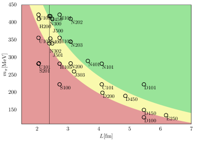
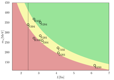
Finally, Figure 3 shows the spatial extent $L$ of the ensembles. Most production ensembles feature $m_{\pi}L\geq 4$, ensuring that exponentially suppressed volume effects are small. For some parameter sets, smaller volumes to check for and control finite size effects have also been generated.

2 Autocorrelation times towards the physical point

In this section we will provide a brief update on estimated autocorrelation times for the Yang-Mills action density at flow time $t_{0}$ determined by the condition $t^{2}\langle E\rangle=0.3$ Luscher:2010iy . While the open boundary conditions in time Luscher:2011kk avoid topological freezing at fine lattice spacing $a$, it is expected that the autocorrelation time in this observable increases significantly as the lattice spacing is decreased. In a previous global fit Bruno:2014jqa of data from the initial set of 2+1 flavor CLS ensembles, the autocorrelation time was determined to be well described by $\tau_{\mathrm{exp}}=14(3)\frac{t_{0}}{a^{2}}$.

(a) N203
$\tau_{\mathrm{int}}=60(32)$ MDU

(b) N302
$\tau_{\mathrm{int}}=49(22)$ MDU

(c) J501
$\tau_{\mathrm{int}}=150(98)$ MDU

Figure 4: History of the YM action density at flow time $t_{0}$ along the MD trajectory.The three panes show results for $a\approx 0.064$fm (a), $a\approx 0.050$fm (b), and $a\approx 0.039$fm (c).

(a) N203
$\tau_{\mathrm{int}}=60(32)$ MDU

(b) N200
$\tau_{\mathrm{int}}=45(21)$ MDU

(c) D200
$\tau_{\mathrm{int}}=101(55)$ MDU

Figure 5: History of the YM action density at flow time $t_{0}$ along the MD trajectory.The three panes show results at fixed lattice spacing $a\approx 0.064$fm for $m_{\pi}\approx 340$ MeV (a), $m_{\pi}\approx 280$ MeV (b), and $m_{\pi}\approx 200$ MeV (c).

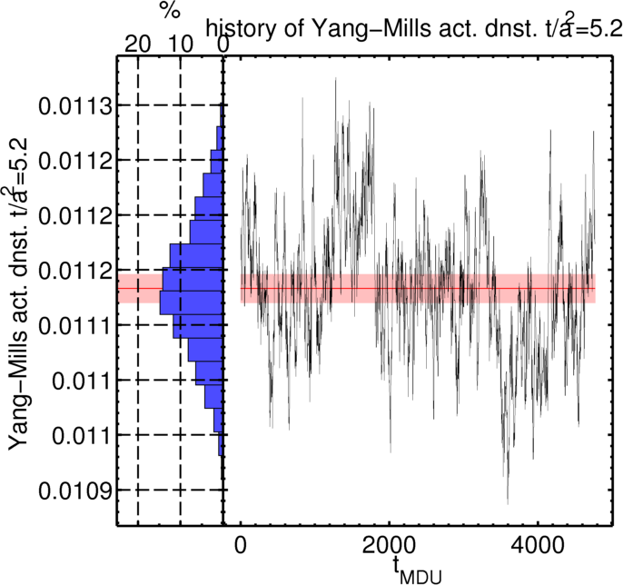
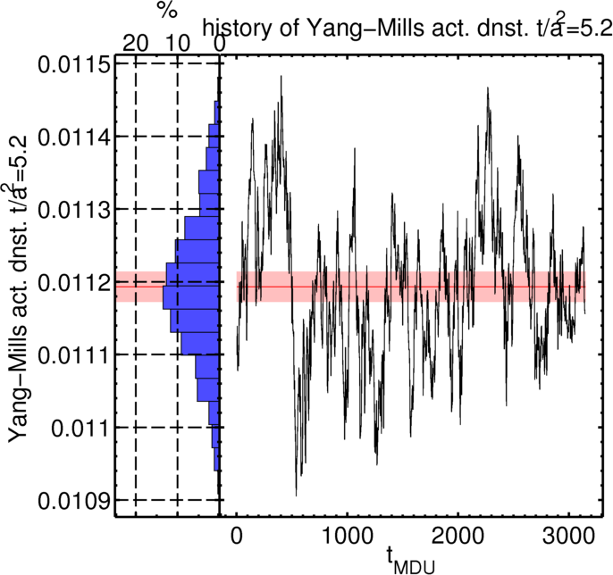
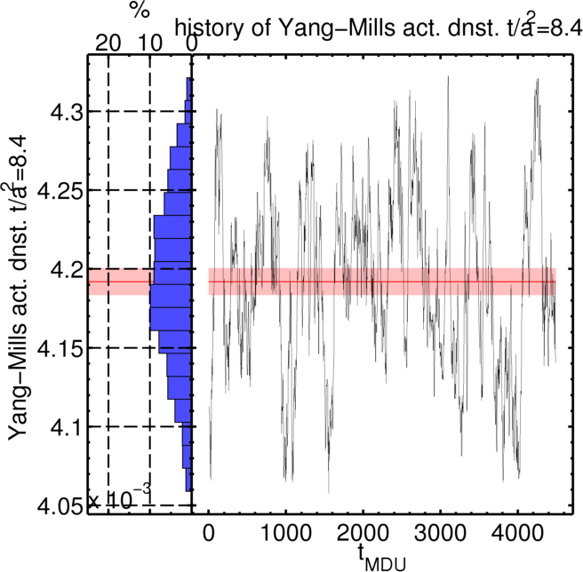
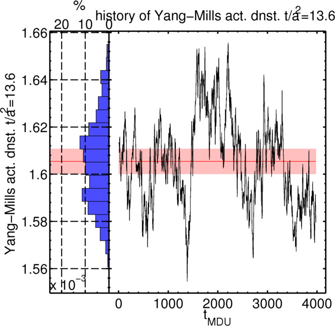
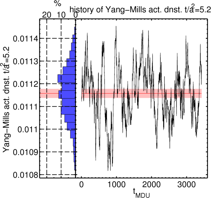
Figure 4 shows the MD history of the YM action density at flow time $t_{0}$ for fixed pion mass $m_{\pi}\approx 340$ MeV and for three lattice spacings. The corresponding integrated autocorrelation time $\tau_{\mathrm{int}}$ is given above each subfigure. Even with chains longer than 3000 MDU the statistical uncertainty on $\tau_{int}$ is large. The current results are consistent with the expected increase of the autocorrelation time Bruno:2014jqa . Figure 5 shows the MD history of the YM action density at flow time $t_{0}$ for three different pion masses along the trajectory with $\operatorname{Tr}(M)=\mathrm{const}$. Unlike in simulations by the MILC collaboration at fixed strange-quark mass Bernard:2017npd , no clear pattern is seen with our current statistics.

3 Thermalization of a physical light-quark mass ensemble

While the current CLS 2+1 flavor ensembles cover a wide range of parameters, the accurate determination of some quantities of phenomenological interest are currently limited by our control of systematic uncertainties associated with the chiral extrapolation. An important example is the calculations of the hadronic contributions to the anomalous magnetic moment of the muon (see DellaMorte:2017dyu for a CLS based determination). Beyond specific observables, our determination of the lattice scale Bruno:2016plf would also greatly benefit from simulations with physical light- and strange-quark masses.

In these proceedings we report on our efforts to thermalize an ensemble (E250) at physical light- (mass degenerate up and down) and strange-quark mass and with $\beta=3.55$ corresponding to a lattice spacing $a\approx 0.064$ fm. At this lattice spacing, the exponential autocorrelation time $\tau_{exp}$ is not yet completely dominated by topology, and therefore periodic boundary conditions are chosen. To keep $m_{\pi}L\geq 4$, we choose a lattice volume $T\times L^{3}=192\times 96^{3}a^{4}$. We work with the following thermalization strategy:

• Start from an $\operatorname{SU}(3)$ run with $T\times L^{3}=64\times 48^{3}a^{4}$, 3 mass-degenerate light quarks and periodic boundary conditions generated for non-perturbative renormalization. Perform a number of runs (updating the light- and strange-quark hopping parameters to their target values ) and thermalize this small volume.

• Triple the time extent and partially thermalize this intermediary ensemble of size $192\times 48^{3}a^{4}$.

• Double the spatial extent and thermalize the resulting ensemble of size $192\times 96^{3}a^{4}$.

3.1 Status of gauge field generation for E250

The thermalization runs on the small and intermediate volume have been successfully completed and we are currently producing a first production chain. At the time of Lattice2017, there was a chain of 436 MDU, corresponding to 109 saved configurations, some of which might not be fully thermalized. The measured acceptance is $0.872(27)$. Figure 6 shows plots for the history of the hamiltonian deficit $\Delta H$ seen in the Monte-Carlo accept/reject step, for the average plaquette, and for the topological charge at the center of the lattice. While a proper analysis will need a much longer Monte-Carlo chain, the right panel of of Figure 6 suggests that at this lattice spacing, the slowing down of topological tunneling is not yet a serious issue.

Figure 6: Left pane: MD history of $\Delta H$ for the physical mass run E250. Mid pane: MD history of the average plaquette. Right pane: History of the topological charge at the center of the lattice.

Figure 7: Reweighting factors for a subset of the configuration produced of E250. Fluctuations in the reweighting factor associated with the rational approximation are very mild (left pane; red). The reweighting factor for the twisted mass reweighting (right pane; black) shows larger fluctuations.

Figure 8: Left pane: Pion correlator from 70 configurations of E250. Right pane: Corresponding effective mass. For details of the correlator construction please refer to the text.

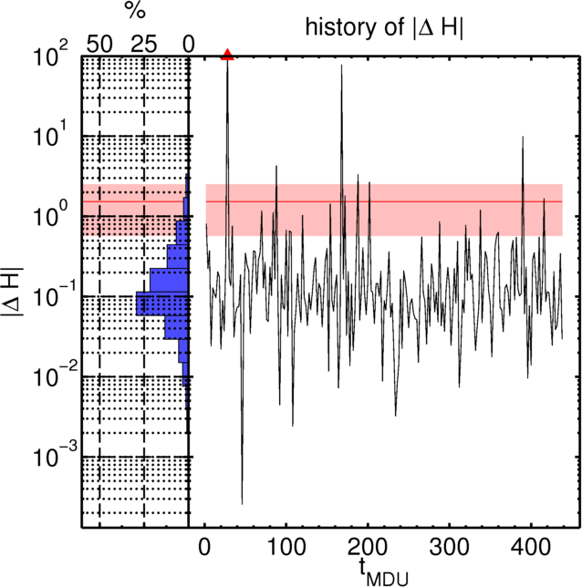
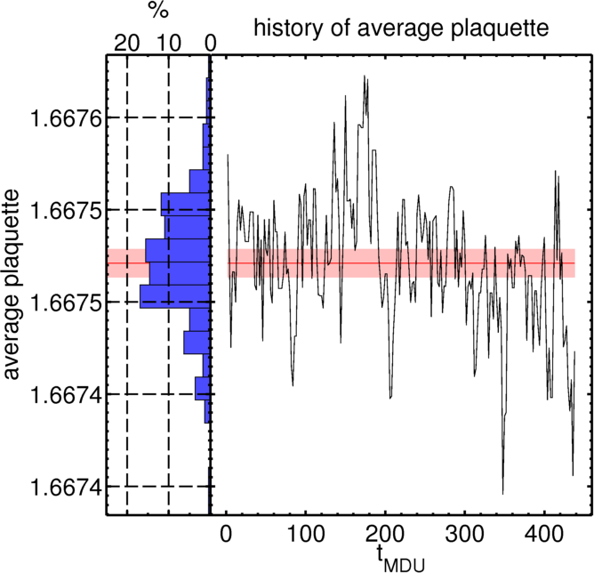
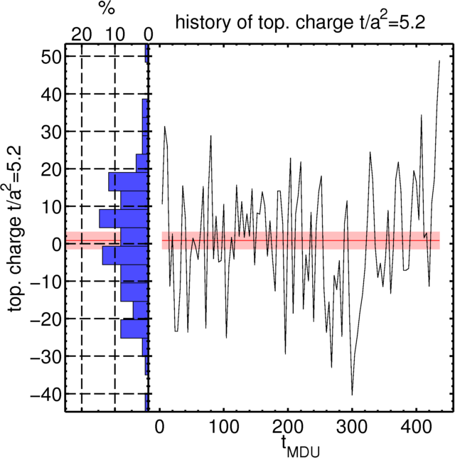
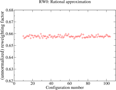
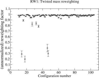
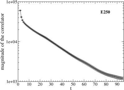
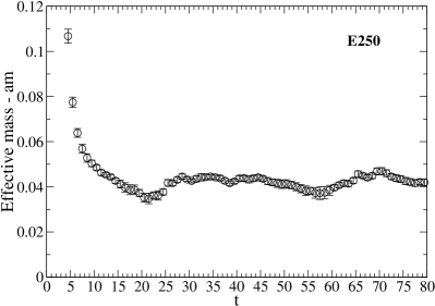
Figure 7 shows the reweighting factors associated with the rational approximation for the strange quark and for the reweighting to zero twisted mass. The reweighting factor for the twisted mass reweighting is estimated using 24 random sources and no intermediate value for the twisted mass parameter $\mu$. For the full ensemble, this estimate might have to be improved, as occasional small reweighting factors are not estimated very accurately.

Figure 8 shows results for the pion correlator and pion effective mass using random wall sources on the same time slice for 70 configurations. With this procedure, autocorrelations in the pion correlator are clearly visible. For future measurements we will make use of the large time extent of the lattice and the periodic boundary conditions by randomly shifting source locations. The current results indicate $m_{\pi}\approx 130(3)$ MeV, reasonably close to the physical pion in the isospin limit and without electromagnetic contributions Aoki:2013ldr , with a mass of $134.8(3)$ MeV.

3.2 Challenges encountered during the thermalization

The initial thermalization runs with $T\times L^{3}=64\times 48^{3}a^{4}$ proceeded smoothly. The same was the case for runs at intermediate volume, which needed various minor parameter adjustments, such as more frequent updates of the deflation subspace along the MD trajectory. Switching to the large volume with $T\times L^{3}=192\times 96^{3}a^{4}$, which was an unprecedented lattice size for CLS simulations using the openQCD Software, a change to a large deflation blocksize was needed in order to maintain a manageable size of the little Dirac operator. While the deflation subspace for CLS runs in smaller volumes is typically of order $4^{3}\times 8$ we had to use a much larger blocksize ($8\times 4\times 8^{2}$) to achieve a stable run. For this setup the resulting iteration counts are somewhat higher than desirable, as deflation is not as efficient. This indicates that a multigrid setup with 3 levels might be preferable for this lattice volume. Such a setup is currently not possible with openQCD. For even larger lattices further algorithmic improvements or a paradigm shift on how lattice QCD simulations are carried out Luscher:2017cjh would be needed.

4 Conclusions and Outlook

The CLS consortium continues its effort to produce a large library of high-quality 2+1 flavor gauge configurations Bruno:2014jqa ; Bali:2016umi . As part of this effort we started production of an ensemble with lattice spacing $a\approx 0.064$ fm and (close-to) physical light- and strange-quark masses. This ensemble will play a crucial role in reducing systematic uncertainties for ongoing projects within the CLS consortium. Examples of such projects (with a focus on activities by the Mainz group) include calculation of the hadronic contribution to $a_{\mu}$ Wittig:2017lat ; Gerardin:2017lat , ongoing baryon structure calculations Djukanovic:2016ocj , a program on lattice spectroscopy and scattering Hoerz:2017lat , and high precision scale setting Bruno:2016plf . While no significant issues were encountered during thermalization, simulations with a large lattice volume, such as E250, might profit from a 3 level multigrid setup not currently available within the openQCD package.

References

- (1) M. Lüscher, S. Schaefer, JHEP 07, 036 (2011), 1105.4749
- (2) M. Lüscher, S. Schaefer, Comput. Phys. Commun. 184, 519 (2013), 1206.2809
- (3) M. Bruno et al., JHEP 02, 043 (2015), 1411.3982
- (4) G.S. Bali, E.E. Scholz, J. Simeth, W. SÃldner (RQCD), Phys. Rev. D94, 074501 (2016), 1606.09039
- (5) http://luscher.web.cern.ch/luscher/openQCD/
- (6) M. Hasenbusch, Phys. Lett. B519, 177 (2001), hep-lat/0107019
- (7) A.D. Kennedy, I. Horvath, S. Sint, Nucl. Phys. Proc. Suppl. 73, 834 (1999), hep-lat/9809092
- (8) M. Lüscher, JHEP 07, 081 (2007), 0706.2298
- (9) M. Lüscher, JHEP 12, 011 (2007), 0710.5417
- (10) R.C. Brower, T. Ivanenko, A.R. Levi, K.N. Orginos, Nucl. Phys. B484, 353 (1997), hep-lat/9509012
- (11) M. LÃscher, JHEP 08, 071 (2010), [Erratum: JHEP03,092(2014)], 1006.4518
- (12) C. Bernard, D. Toussaint (MILC) (2017), 1707.05430
- (13) M. Della Morte, A. Francis, V. GÃlpers, G. HerdoÃza, G. von Hippel, H. Horch, B. JÃger, H.B. Meyer, A. Nyffeler, H. Wittig, JHEP 10, 020 (2017), 1705.01775
- (14) M. Bruno, T. Korzec, S. Schaefer, Phys. Rev. D95, 074504 (2017), 1608.08900
- (15) S. Aoki et al., Eur. Phys. J. C74, 2890 (2014), 1310.8555
- (16) M. LÃscher, Stochastic locality and master-field simulations of very large lattices, in 35th International Symposium on Lattice Field Theory (Lattice 2017) Granada, Spain, June 18-24, 2017 (2017), 1707.09758, http://inspirehep.net/record/1613675/files/arXiv:1707.09758.pdf
- (17) H. Wittig et al., A lattice calculation of the hadronic vacuum polarization contribution to , in Proceedings, 35th International Symposium on Lattice Field Theory (Lattice2017): Granada, Spain, indico ID 392, to appear in EPJ Web Conf.
- (18) A. Gérardin et al., Light-by-light forward scattering amplitudes in Lattice QCD, in Proceedings, 35th International Symposium on Lattice Field Theory (Lattice2017): Granada, Spain, indico ID 373, to appear in EPJ Web Conf.
- (19) D. Djukanovic, T. Harris, G. von Hippel, P. Junnarkar, H.B. Meyer, H. Wittig, PoS LATTICE2016, 167 (2017), 1611.07918
- (20) J. Bulava, B. Hörz, C. Morningstar, Multi-hadron spectroscopy in a large physical volume, in Proceedings, 35th International Symposium on Lattice Field Theory (Lattice2017): Granada, Spain, indico ID 308, to appear in EPJ Web Conf, arXiv:1710.04545.