A study of elliptic PDEs with jump diffusion coefficients ]A. Barth and A. Stein
A study of elliptic partial differential equations with jump diffusion coefficients
Abstract
As a simplified model for subsurface flows elliptic equations may be utilized. Insufficient measurements or uncertainty in those are commonly modeled by a random coefficient, which then accounts for the uncertain permeability of a given medium. As an extension of this methodology to flows in heterogeneous\fractured\porous media, we incorporate jumps in the diffusion coefficient. These discontinuities then represent transitions in the media. More precisely, we consider a second order elliptic problem where the random coefficient is given by the sum of a (continuous) Gaussian random field and a (discontinuous) jump part. To estimate moments of the solution to the resulting random partial differential equation, we use a pathwise numerical approximation combined with multilevel Monte Carlo sampling. In order to account for the discontinuities and improve the convergence of the pathwise approximation, the spatial domain is decomposed with respect to the jump positions in each sample, leading to path-dependent grids. Hence, it is not possible to create a sequence of grids which is suitable for each sample path a-priori. We address this issue by an adaptive multilevel algorithm, where the discretization on each level is sample-dependent and fulfills given refinement conditions.
keywords:
Adaptive multilevel Monte Carlo method, flow in heterogeneous media, fractured media, porous media, jump-diffusion coefficient, non-continuous random fields, elliptic equation60H25, 60H30, 60H35, 35R60, 65C05 , 58J65
1 Introduction
Uncertainty quantification plays an increasingly important role in a wide range of problems in the Engineering Sciences and Physics. Examples of sources of uncertainty are imprecise or insufficient measurements and noisy data. In the underlying dynamical system this is modeled via a stochastic operator, stochastic boundary conditions and/or stochastic data. As an example, to model subsurface flow more realistically the coefficient of an (essentially) elliptic equation is assumed to be stochastic. A common approach in the literature is to use (spatially) correlated random fields that are built from uniform distributions or colored log-normal fields. The resulting marginal distributions of the field are (shifted) normally, resp. log-normally distributed. Neither choice is universal enough to accommodate all possible types of permeability, especially not if fractures are incorporated (see [39]), the medium is very heterogeneous or porous.
The last decade has been an active research period on elliptic equations with random data. A non-exhaustive list of publications in this field includes [1, 8, 9, 12, 19, 20, 25, 31, 33, 37, 38]. One can find various ways to approximate the distribution or moments of the solution to the elliptic equation. Next to classical Monte Carlo methods, their multilevel variants and other variance reduction techniques have been applied. The concept of multilevel Monte Carlo simulation has been developed in [29] to calculate parametric integrals and has been rediscovered in [26] to estimate the expected value of functionals of stochastic differential equations. Ever since, multilevel Monte Carlo techniques have been successfully applied to various problems, for instance in the context of elliptic random PDEs in [1, 12, 19, 31, 38] to just name a few. These sampling algorithms are fundamentally different from approaches using Polynomial Chaos. The latter suffer from the fact that one is rather restricted when it comes to possibilities to model the stochastic coefficient. While in the case of fields built from uniform distributions or colored log-normal fields these algorithms can outperform sampling strategies, approaches – like stochastic Galerkin methods – are less promising in our discontinuous setting due to the rather involved structure of the coefficient. In fact, it is even an open problem to define them in the case that a Lévy-field is used.
Our main objective in this paper is to show existence and uniqueness of the solution to the elliptic equation when the coefficient is modeled as a jump-diffusion. By that we mean a field which consists of a deterministic, a Gaussian and non-continuous part. As we show in the numerical examples, this jump-diffusion coefficient can be used to model a wide array of scenarios. This generalizes the work in [31] and uses partly [30]. To approximate the expectation of the solution we develop and test, further, variants of the multilevel Monte Carlo method which are tailored to our problem: namely adaptive and bootstrapping multilevel Monte Carlo methods. Adaptivity is needed in the jump-diffusion setting, since the coefficient is not continuous. Our analysis shows that the non-adaptivity in a multilevel setting with non-continuous coefficients entails a larger error than when an adaptive algorithm is used. This result is not surprising, since the essence of the multilevel algorithm is that many samples are calculated on coarse grids, where the distributional error from misjudging jump-locations is high. Adaptivity, however, comes to the price that in certain scenarios solving the underlying system of equation becomes computationally expensive. In these settings the advantageous time-to-error performance of adaptive methods may be worse. Bootstrapping, as a simplified version of Multifidelity Monte Carlo sampling (see [34]), reuses samples across levels and is preferred when sampling from a certain distribution is computationally expensive. The bootstrapping algorithms outperform, in general, algorithms with a standard sampling strategy of multilevel Monte Carlo, as it actually reduces the mean square error.
In Section 2 we introduce the model problem, define pathwise weak solutions of random partial differential equations (PDEs) and show almost sure existence and uniqueness under relatively weak assumptions on the model parameters. The main contribution of this section is the existence and uniqueness result in Theorem 2.5, which is then readily transferred to the special case of a jump-diffusion problem in the subsequent sections of this article. In Section 3 we define the jump-diffusion coefficient and construct suitable approximations. Both stochastic parts of the jump-diffusion coefficient are approximated: The Gaussian one by a standard truncation of its basis representation, and the jump part (if direct sampling from the jump distribution is not possible) by a technique based on Fourier Inversion. We show -type convergence for all existing moments of the approximation. From this result convergence of the approximated solution follows immediately. The approximated solution has still to be discretized to actually estimate moments of it (Section 4). The Galerkin-type discretization is directly furthered into an adaptive scheme. Section 5 then introduces the sampling methods that are used, namely Monte Carlo, multilevel Monte Carlo and a bootstrapping variant of it. An extensive discussion of numerical examples in one and two dimensions, in Section 6, concludes the paper.
2 Elliptic boundary value problems and existence of solutions
We consider the following random elliptic equation in a general setting before we specify in Section 3 our precise choice of coefficient function. Let be a complete probability space and , for some , be a bounded and connected Lipschitz domain. In this paper we consider the linear, random elliptic problem
| (2.1) |
where is a stochastic jump-diffusion coefficient and is a random source function. The Lipschitz boundary consists of open -dimensional manifolds which are grouped into two disjoint subsets and such that and . We impose mixed Dirichlet-Neumann boundary conditions
| (2.2) | ||||
on Eq. (2.1), where is the outward unit normal vector to and , assuming that the exterior normal derivative on is well-defined for any . To obtain a pathwise variational formulation of this problem, we use the standard Sobolev space equipped with the norm
where denotes the Euclidean norm on . On the Lipschitz domain , the existence of a bounded, linear operator
with
and
| (2.3) |
for and some constant , dependent only on , is ensured by the trace theorem, see for example [22]. At this point, one might argue that the trace operator needs to be defined pathwise for any , since the Neumann part of the boundary conditions in Eq. (2.2) may contain a random function . This is true if one works with on , as the trace then has to match the boundary condition given by ) on for -almost all and . In our case, for simplicity, we may treat independently of , since we only consider the trace operator on the homogeneous boundary part to define as follows: The subspace of with zero trace on is then
with norm
Remark 2.1.
The condition implies that is a closed linear subspace of . We may as well work with non-homogeneous boundary conditions on the Dirichlet part, i.e. for . The corresponding trace operator is still well defined if, for -a.e. , can be extended to a function . Then, we consider for -a.e. the problem
But this is in fact a version of Problem (2.1) equipped with Eqs. (2.2) where the source term and Neumann-data have been changed (see also [24, p. 317]).
As the coefficient and the boundary conditions are given by random functions, the solution is also a random function. Besides pathwise properties, may also have certain integrability properties with respect to the underlying probability measure. To this end, we introduce the space of Bochner integrable random variables resp. random functions (see [21] for an overview).
Definition 2.2.
Let be a Banach space and define the norm for a -valued random variable as
The corresponding space of Bochner-integrable random variables is then given by
The following set of assumptions on and allows us to show existence and uniqueness of the solution to Eq. (2.1). Consequently, we denote by the topological dual of a vector space .
Assumption 2.3.
Let . For -almost all it holds that:
-
•
and .
-
•
, and for some such that .
Remark 2.4.
In Assumption 2.3, we did not establish a uniform elliptic bound on in (see for example [31]), neither did we assume a certain spatial regularity as in [17, 38]. The relatively weak assumptions are natural in our context, since in Section 3 we model as a jump-diffusion coefficient and uniform bounds or assumptions on Hölder-continuity are too restrictive. For the investigation of problem (2.1) with piecewise Hölder-continuous coefficients we refer to [38]. We may identify with its dual and work on the Gelfand triplet . Hence, Assumption 2.3 guarantees that , and, similarly, for -almost all .
For fixed , multiplying the random PDE (2.1) with a test function and integrating by parts yields the integral equation
| (2.4) |
Consider the bilinear form
and
where the integrals in are understood as the duality pairings
Equation (2.4) then leads to the pathwise variational formulation of Problem (2.1):
For -almost all , given and , find such that
| (2.5) |
for all . A function that fulfills the pathwise variational formulation is then called pathwise weak solution to Problem (2.1).
Theorem 2.5.
Proof.
Choose such that Assumption 2.3 is fulfilled. For all , we obtain by the Cauchy-Schwarz inequality
On the other hand,
where the constant stems from the constant in Poincaré’s inequality, , and only depends on . Hence the bilinear form is continuous and coercive. We use that and the trace theorem (Equation (2.3)) to bound by
This shows that is a bounded linear functional on (and therefore continuous) for almost all . The existence of a unique pathwise weak solution is then guaranteed by the Lax-Milgram lemma -almost surely. If is a solution of Eq. (2.5) for given and , then
Using Hölder’s and Minkowski’s inequality together with yields:
In the next section, we introduce the diffusion coefficient , which allows us to incorporate discontinuities at random points or areas in . We show the existence and uniqueness of a weak solution to the discontinuous diffusion problem by choosing such that Assumption 2.3 is fulfilled and Theorem 2.5 may be applied.
3 Discontinuous random elliptic problems
The stochastic coefficient in a jump-diffusion model should incorporate random discontinuities as well as a Gaussian component. We achieve this characteristic form of by defining the coefficient as a Gaussian random field with additive discontinuities on random areas of . Since this usually involves infinite series expansions in the Gaussian component or sampling errors in the jump measure, we also describe how to obtain tractable approximations of . Subsequently, existence and uniqueness results for weak solutions of the unapproximated resp. approximated jump-diffusion problem based on the results in Section 2 are proved. We conclude this section by showing pathwise and -convergence of the approximated solution to the solution to the (unapproximated) discontinuous diffusion problem.
3.1 Jump-diffusion coefficients and their approximations
Definition 3.1.
The jump-diffusion coefficient is defined as
| (3.1) |
where
-
•
is non-negative, continuous and bounded.
-
•
is a continuously differentiable, positive mapping.
-
•
is a (zero-mean) Gaussian random field associated to a non-negative, symmetric trace class operator .
-
•
is a finite measure on and is a random partition of with respect to . The number of elements in is a random variable on with .
-
•
is a sequence of non-negative random variables on and
The sequence is independent of (but not necessarily i.i.d.).
Remark 3.2.
The definition of the measure on in Def. 3.1 relates not only to the average number of partition elements , but may further be utilized to concentrate discontinuities of the jump-diffusion coefficient to certain areas of . Choosing, for instance, as the Lebesgue measure on corresponds to uniformly distributed jumps and on average equally sized partition elements . In contrast, if is a Gaussian measure on around some center point , the number of discontinuities (resp. size of partition elements) will decrease (resp. increase) as one moves away from . We refer to the numerical experiments in Section 6, where we give interpretations of to model certain characteristics of different jump-diffusion coefficients. On a further note, we do not require stochastic independence of and .
In general, the structure of as in Def. 3.1 does not allow us to draw samples from the exact distribution of this random function. For an approximation of the Gaussian field, one usually uses truncated Karhunen-Loève expansions: Let denote the sequence of eigenpairs of , where the eigenvalues are given in decaying order . Since is trace class the Gaussian random field admits the representation
where is a sequence of independent and standard normally distributed random variables. The series above converges in and -almost surely (see i.e. [3]). The truncated Karhunen-Loève expansion of is then given by
where we call the cut-off index of . In addition, it may be possible that the sequence of jumps cannot be sampled exactly but only with an intrinsic bias (see also Remark 3.4). The biased samples are denoted by and the error which is induced by this approximation is represented by the parameter as in Assumption 3.3. To approximate using the biased sequence instead of we define the jump part approximation
The approximated jump-diffusion coefficient is then given by
| (3.2) |
and the corresponding stochastic PDE with approximated jump-diffusion coefficient reads
| (3.3) | ||||
For and given samples and , we consider the pathwise weak solution to Problem (3.3) for fixed approximation parameters and . The variational formulation of Eq. (3.3) is then analogous to Eq. (2.5) given by: For almost all with given , , find such that
| (3.4) |
for all . The following assumptions guarantee that we can apply Theorem 2.5 also in the jump-diffusion setting and that therefore pathwise solutions and exist.
Assumption 3.3.
-
(i)
The eigenfunctions of are continuously differentiable on and there exist constants such that for any
-
(ii)
Furthermore, the mapping as in Definition 3.1 and its derivative are bounded by
where with and are arbitrary constants.
-
(iii)
Given and , there exists a such that and .
-
(iv)
Finally, for some , consists of -integrable random variables, i.e. for all and , further there exists a sequence of approximations so that the sampling error is bounded, for , by
Remark 3.4.
Assumption 3.3 (i) on the eigenpairs of is natural. For instance, the case that is a Brownian-motion-like random field or that is a Matérn covariance operator are included. The bounds on and the regularity assumptions on and (Assumption 3.3 (ii),(iii)) are necessary to ensure that the solution has at least finite expectation. The sampling error in Assumption 3.3 (iv) may be interpreted in several ways: For instance, it may account for uncertainties in the distribution of , like parameters for which only confidence intervals are available. Another possibility is, that realizations of may not be simulated directly or only at relatively high computational costs, for example by Acceptance Rejection algorithms, see [5, Chapter II]. In this case, it may be favorable to generate the approximation by a more efficient numerical algorithm (i.e. Fourier inversion techniques, see [13]) instead and to control for the error. The resulting sampling error can then be equilibrated with the truncation error from the Gaussian field to achieve a desired overall accuracy.
3.2 Existence of and
We first show the existence of a weak solution for both, the jump-diffusion problem (2.1) with as in Definition 3.1, and the approximated problem (3.3).
Lemma 3.5.
Proof.
By Theorem 2.5, it is sufficient to show that and fulfill Assumption 2.3. Clearly, for almost all , as and are non-negative and we have the lower bound on in Assumption 3.3 (ii) by definition. Consequently, it is sufficient to bound the expectation of , for , from below (see also [16, Section 2.3]).
The random variable follows a centered normal distribution for any . To see this, consider the finite sum
for and a sequence of i.i.d. -distributed random variables. Clearly, is normally distributed with zero mean and characteristic function
Using that is trace class with for all and , it follows
and hence
where the right hand side is the characteristic function of a normal distribution with zero mean and variance . By the Lévy continuity theorem this implies that
for all . Next we show that has -almost surely Hölder continuous paths (see also [16, Proposition 3.4]): Let (where are defined in Ass. 3.3 (i)) and . For and any we have
where and the constant stems from Ass. 3.3 (i). The second equality results from the fact that for all and the sum in the inequality is finite because . For any dimension , we may choose and obtain by the Kolmogorov-Chentsov theorem ([21, Theorem 3.5]) that has a Hölder continuous modification with Hölder exponent . Hence, is a centered Gaussian process and almost surely bounded on . By [2, Theorem 2.1.1] this implies and
| (3.5) |
for all and . With Assumption 3.3 (ii) and since we further obtain
By Fubini’s Theorem and integration by parts we may bound
where we have used , by the symmetry of , and Ineq. (3.5) in the last step. The last expectation is finite if and only if . For this to hold, is sufficient, since and thus .
Remark 3.6.
From Lemma 3.5 follows immediately that one cannot expect finite second moments of the solution for or . If we assume that we need to have finite second moments (in the case of, for instance, a log-normal Gaussian field). Note that, for all covariance kernels and functionals we use (e.g. log-Gaussian fields with Matérn class covariance or Brownian-motion like covariance kernels), and are much smaller than . If one assumes that , and are stochastically independent, then the regularity of the solution (in ) is at least the same as the lowest regularity of the data, i.e. , or .
Lemma 3.7.
Proof.
The proof is carried out identically to Lemma 3.5, where we replace by , by , by and by . Again, by Eq. (3.2), -almost surely. In the case that , the random field is degenerated and equal to zero. Hence, for all and the claim follows immediately. Otherwise, if , we obtain in the fashion of Lemma 3.5
which is again finite if . The proof is concluded by noting that the last estimate is independent of and .
3.3 Convergence of the approximated diffusion coefficient
The convergence of the approximated solution to depends on the convergence of the approximated jump-diffusion coefficient to . We investigate this convergence by deriving separately convergence rates of the truncated Karhunen-Loève series and the approximation of the jump part.
Theorem 3.8.
In order to prove the bound for the truncation error, we need the following Fernique-type result.
Theorem 3.9.
[32, Theorem 2.9] Let with be a centered Gaussian field. For let
Then for all
where is the inverse function of , is an absolute constant and .
Proof of Theorem 3.8.
With a similar continuity argument as in Lemma 3.5, we obtain that
where for all . Hence
and we see by the proof of Lemma 3.5 that for as in Theorem 3.9
for any and each . We use the estimate on to bound for by
Since and are monotone increasing this yields with Theorem 3.9 for any
Using again that and Fubini’s Theorem, we have for any
where is the Gamma function and we have used the substitution in the second equality. This proves the claim because the above estimate holds for any .
Remark 3.10.
In [16], the author proves a similar error bound for the truncation error in the Gaussian field, namely
In the jump-diffusion setting the error bound in Theorem 3.8 is advantageous for several reasons:
-
•
In our setting, will in general not have Hölder continuous paths, but involves discontinuities, hence only the error in is of interest.
-
•
In general it is rather easy to calculate the sum if the first eigenvalues are known (or can be approximated), whereas this is not necessarily the case for .
Theorem 3.11.
Proof.
For any , we have
By Fubini’s Theorem and integration by parts this yields
since . For fixed and , we define the sets
to obtain the identity
By the independence of and this yields
and thus by Fubini’s theorem
The claim then follows since by Definition 3.1.
Theorem 3.12.
Let Assumption 3.3 hold, then there exists a constant , depending only on the indicated parameters, such that for any and
Hence, converges to in as and .
Proof.
Let and be fixed. By the mean-value theorem
where . With Assumption 3.3 (ii) on and by the triangle inequality, we obtain the estimate
The random fields and are independent, so for any it holds that
| (3.6) |
where we have used Hölder’s inequality with such that . With Young’s inequality we obtain
Since with , we proceed as in Lemma 3.5 and conclude by Fernique’s theorem that and note that is independent of . Similarly,
for any and is independent of . Altogether, this yields
Corollary 3.13.
Let Assumption 3.3 hold, then there exists a sequence of approximation parameters in , depending only on and , such that the error converges to zero -almost surely as .
3.4 Convergence of the approximated solution.
We conclude this section by showing the convergence of towards , given that in .
Theorem 3.14.
Proof.
Existence and uniqueness of weak solutions resp. , for , is guaranteed by Lemma 3.5 resp. Lemma 3.7 -almost surely. For notational convenience, we omit the argument in the following pathwise estimates with respect to the norm . With Poincaré’s inequality and -a.s., we obtain the (pathwise) estimate
where denotes the Poincaré constant. Since and are weak solutions of Problem (2.1) with Eq. (2.2) resp. Eq. (3.3), we have
almost surely, and hence
By Hölder’s inequality, , Eq. (2.3) and Theorem 2.5 we have
Using , the -th moment of the pathwise error is bounded by
| (3.7) |
where is as in Theorem 2.5. The convergence now follows by Theorem 3.12, since is bounded uniformly in and by Lemma 3.7.
Corollary 3.15.
With the Assumptions of Theorem 3.14, there exists a sequence of approximation parameters in , depending only on and , such that converges to zero -almost surely as .
Proof.
Knowing that converges to pathwise and in , we aim to estimate moments of by drawing samples from the distribution of . In general, the distribution of is not known. Further, each pathwise solution is an element of the infinite-dimensional Hilbert space , which in turn means that we are only able to simulate pathwise approximations of the functions in a finite-dimensional subspace of . Next, we show how to construct these approximations in some appropriate subspaces of and how the discretization error may be controlled.
4 Adaptive pathwise discretization
The variational problem (3.4) to Eq. (3.3) is to find for almost all and given , , and a function such that
| (3.4) |
for all . To find suitable approximations of , we use a standard Galerkin approach with a sequence of finite-dimensional subspaces . The corresponding family of refinement sizes is given by a sequence , which decreases monotonically to zero as . For any , let and be a basis of . The discrete version of the variational formulation (3.4) is then: Find such that
| (4.1) |
The function may be expanded with respect to the basis as
where and is the respective coefficient (column-)vector. With this, the discrete variational problem in the finite-dimensional space is equivalent to solving the linear system of equations
with stochastic stiffness matrix and load vector for . Since the jump-diffusion coefficient is not continuous, in general one would not expect the full convergence rate of the Galerkin approximation.
Example 4.1.
For a polygonal domain , we define by a sequence of triangulations on . We denote the minimum interior angle of all triangles in by and assume that there exists some such that . The maximum diameter of each triangulation is defined by
and the finite-dimensional subspaces are given by
where is the space of all polynomials up to degree one. This yields a sequence of subspaces in with refinement parameters . For fixed , let be a basis of piecewise linear functions of . Given that for some , the pathwise discretization error is bounded by Céa’s lemma -almost surely by
where is the Poincaré constant and is deterministic and only depends on the indicated parameters (see e.g. [28, Chapter 8.3/8.5]). If is sample-independent (and thus is fixed for any ), and there exists a uniform bound in and , we readily obtain
by Hölder’s inequality. We note that a uniform a-priori bound may require higher moments of , and or even essential bounds on which are not ensured by Assumption 3.3.
Remark 4.2.
For jump-diffusion problems, we obtain, in general, a discretization error of order . We cannot expect the pathwise ”full” order of convergence of the finite-dimensional discretization error, since the diffusion coefficient is almost surely discontinuous. Most results that ensure -regularity of the pathwise weak solution need that is continuously differentiable or that , see for instance [24]. The latter would imply that is continuous by the Sobolev embedding theorem, which contradicts our setting. As we consider pathwise regularity, we can rely on results for deterministic elliptic problems with discontinuous coefficients. We refer to [35] and the references therein, where the author emphasizes that the regularity of the solution depends on the shape and magnitude of the discontinuities. For several examples -regularity with is shown. In [7] the author states that without special treatment of the interfaces with respect to the triangulation one, in general, cannot expect a better pathwise convergence rate than .
4.1 Adaptive triangulations
In view of the previous remark, we aim to increase the order of convergence with respect to . For this, we employ path-dependent triangulations to match the interfaces generated by the samples of the jump-diffusion coefficient. Hence, we need to reformulate the discrete problem with respect to , since the triangulation and matching basis functions may be sample-dependent. Given a fixed and , we consider a finite-dimensional subspace with sample-dependent basis and stochastic dimension . As before, we denote by the sequence of (random) refinement parameters corresponding to the sequence of subspaces . To be more precise, for a given random partition of , we choose a triangulation of with respect to such that
where is a positive sequence of deterministic refinement thresholds, decreasing monotonically to zero. This guarantees that almost surely, although the absolute speed of convergence may vary for each . Denoting by the minimal interior angle within , we assume similarly to Example 4.1 that there exists a such that for -almost all
| (4.2) |
The pathwise discrete variational problem in the sample-adaptive subspace now reads: Find such that
| (4.3) |
Since the triangulation is aligned with the discontinuities of , this approximation admits an increase of the (pathwise) order of convergence compared to the non-adaptive, deterministic Galerkin approximations. For piecewise linear basis functions , we can expect
| (4.4) |
-a.s. by results from domain decomposition methods for deterministic elliptic problems (e.g. [14, 15]). We emphasize that with the assumption of Eq. (4.2) the constant is independent of . This estimate holds provided the random partitions are polygonal and is almost surely piecewise in . In this case, the adaptive triangulations perfectly fit the random subdomains in and the order of convergence is the same as if . If the random partitions are not polygonal but form -interfaces within , we obtain log-linear rates:
| (4.5) |
Remark 4.3.
Based on Ass. 4.4 and the pathwise estimates in Eqs. (4.4), (4.5), the question arises whether it is possible to derive estimates in a mean-square sense
where the constant is independent of and . As the independence of is not an issue, a uniform estimate with respect to requires further summability conditions (i.e. ) on the eigenvalues in Ass. 3.3 and would result in a piecewise differentiable diffusion coefficient . To illustrate this, we consider the identity
on some partition element . Rearranging terms and taking expectations then yields by Hölder’s inequality
If and have sufficiently high moments and the eigenvalues decay fast enough, the right hand side may be bounded uniformly with respect to , then it is straightforward to derive the corresponding -estimates. These assumptions, however, exclude the important cases where the covariance operator of is of Brownian-motion-type or exponential. Practically, as we show in Section 6, the pathwise adaptive convergence rates may also be recovered for the -error if has only piecewise Hölder-continuous trajectories.
In view of the preceding remarks and Example 4.1, we make the following assumption on the mean-square discretization error:
Assumption 4.4.
There exist constants , such that for any and , the finite-dimensional approximation errors of in the subspaces resp. are bounded by
The constants may depend on and , but are independent of and .
Note that in general by the previous observations. We consider instead of as both quantities depend to a great extend on the geometry introduced by . The parameter has been merely introduced to ensure that .
5 Estimation of expectations by Monte Carlo methods
As we are able to generate samples from and control for the discretization error in each sample, we may estimate the expected value of the weak solution to Eq. (2.1). We focus on multilevel Monte Carlo estimators as they are easily implemented and do not require much regularity of . Monte Carlo estimators introduce an additional statistical bias besides the error contributions of and the pathwise discretization error from Section 4. However, this error can be controlled under natural assumptions and it may be equilibrated according to the other error terms. In this section, we first recall briefly standard Monte Carlo and multilevel Monte Carlo methods to estimate and then control for the mean-squared error in both algorithms. We also suggest a modification of the multilevel Monte Carlo estimation to increase computational efficiency before we verify our results on several numerical examples in Section 6.
5.1 Monte Carlo and multilevel Monte Carlo estimators
Consider a sequence of i.i.d. copies of the -valued random variable . For independent samples, the Monte Carlo estimator of is defined as
Since we are only able to draw samples of the approximated discrete solution as introduced in Section 4, we aim to control the root mean-squared error (RMSE) . For notational convenience, we focus only on the adaptive discretization with mean-square refinement and converge rate in this section. However, all results also hold in the non-adaptive case where we replace by and by . To derive a bound for the RMSE, we need the following standard result.
Lemma 5.1.
Let and . Then
Theorem 5.2.
Proof.
We apply the triangle inequality to obtain
By the first part of Lemma 5.1 and Theorem 2.5, we bound the first term by
The second part of Lemma 5.1 yields with the estimate of Theorem 3.14
where are independent of and , because is bounded uniformly with respect to these parameters by Lemma 3.7. Finally, Assumption 4.4 and Lemma 5.1 yield for the third term
where is also independent of and by assumption.
Remark 5.3.
The estimate in Theorem 5.2 suggests that all four error contributions should be equilibrated to obtain a RMSE of order . For this, we may choose and such that
While this is straightforward for and usually also for , the choice of the truncation index involves a few difficulties. In general, the eigenvalues of the covariance operator will not be available in closed form. The decay parameter may be unknown and only be bounded from below, which would result in an overestimation of the term . One possibility to find is applicable if is an integral operator of the form
with some nonnegative, symmetric and bounded kernel function and . In this case, the eigenvalues of fulfill the identity (see [23, 40]). Operators with this property are widely used in practice and include for instance Matérn class, -exponential and rational quadratic covariance functions (see [36]). The first eigenvalues of have to be, in any case, determined (numerically) to approximate the Gaussian field , so we select such that
In most cases, the sampling of and for given boundary data will be computationally expensive: If the eigenvalues of decay slowly, it is necessary to include a large number of terms in the Karhunen-Loève expansion to achieve . In addition, sampling of the sequence might also be time-consuming if a small error is desired. Given a sample of , one has then to rely on numerical integration schemes to calculate the entries of the stiffness matrix and the load vector , and solve a possibly large system of linear equations. This motivates the use of advanced Monte Carlo techniques, such as multilevel Monte Carlo, to achieve essentially the same accuracy with reduced computational effort. We briefly recall the idea of the multilevel Monte Carlo sampling in the following.
For we consider finite-dimensional subspaces of with refinement sizes and approximation parameters and . We define and expand the “finest level approximation” into a telescopic sum to obtain
Instead of estimating the left hand side by the ordinary Monte Carlo method, we estimate the expected corrections by generating independent realizations on each level and calculating the Monte Carlo estimator . The multilevel Monte Carlo estimator of is then defined as
| (5.1) |
To achieve a desired target RMSE of , this estimator requires less computational effort than the standard Monte Carlo approach under certain assumptions. This, by now, classical result was proven in [26, Theorem 3.1]. The proof is rather general and may readily be transferred to the problem of estimating moments of random PDEs (see [12]).
Theorem 5.4.
Let Assumptions 3.3 and 4.4 hold such that , where for as in Lemma 3.5. For , let , and be the level dependent approximation parameters for any such that are decreasing and is increasing with respect to . Then the multilevel Monte Carlo estimator admits the bound
where is a constant independent of and the level-dependent approximation parameters.
Proof.
Using the triangle inequality and Jensen’s inequality for expectations, we observe that
Theorem 3.14 and Assumption 4.4 give a bound for the first term by
where is an independent constant. For the second error term, the definition of in Eq. (5.1) together with Lemma 5.1 yield
Now, the terms may be treated analogously to :
The remaining term is bounded by Theorem 2.5 via
Finally, we arrive at the estimate
For the last inequality, we have used that and with
Regarding a single realization of , we want the pathwise error to decrease as increases, so naturally the parameters and should decrease in and increase in . For example, by using a sequence of refining grids, the refinement parameter may be divided roughly by a factor of two in each level, i.e. for any . Similar refining factors may be imposed for the sum of the remaining eigenvalues and the sampling errors . One advantage of the multilevel Monte Carlo estimator is that we are now able to even out the error contributions of the sampling bias and the statistical error (with respect to ) on each level. This is achieved by generating relatively few of the accurate, but expensive, samples for large and generating more of the cheap, but less accurate, samples on the lower levels.
Corollary 5.5.
Let the assumptions of Theorem 5.4 hold. For and given refinement parameters choose and such that
and such that for some arbitrary
The RMSE of the corresponding multilevel Monte Carlo estimator is then of order :
Proof.
With the above choice of the approximation parameters and Theorem 5.4, we obtain
where is the Riemann zeta function.
For the level-dependent choice of and we refer to Remark 5.3. In the remainder of this section, we introduce a modification of the multilevel Monte Carlo method to further reduce computational complexity.
5.2 Bootstrapping multilevel Monte Carlo
Recall the multilevel Monte Carlo estimator
of as in Eq. (5.1), where the terms in the second sum are independent copies of the corrections . In total, one has to generate samples of for each (where we have set ). This could be expensive even in low dimensions . We can reduce this effort if we “recycle” the already available samples and generate the differences
based on the same realization for . That is, we drop the second superscript in and arrive at the bootstrap multilevel Monte Carlo estimator
This entails generating realizations of the random variable instead of . The samples are then independent in , but not anymore across all levels for a fixed index . The bootstrap estimator is unbiased, i.e , and it holds
The introduced modification is a simplified version of the Multifidelity Monte Carlo estimator (see [34]). Under suitable assumptions on the variance of , it is shown in [34] that the Multifidelity Monte Carlo approach achieves the same rate of convergence as the standard multilevel Monte Carlo method with reduced computational effort. The bootstrap estimator corresponds to a Multifidelity Monte Carlo estimator where the weighting coefficients for all level corrections are set equal to one.
We emphasize that the error bounds derived in Thm. 5.4 and Cor. 5.5 do not require independence of the sampled differences across the levels . Thus, the asymptotic order of convergence also holds for the bootstrapping estimator. However, we have now introduced additional correlation across the levels, which may entail higher variance, and thus slower convergence of the bootstrapping method. The variance of the standard multilevel Monte Carlo estimator is easily calculated as
whereas
In case that the differences are positively correlated across the levels, we trade in simulation time for a possibly higher RMSE, where the ratio of this trade is problem-dependent and hard to access beforehand. Nevertheless, we will compare this modified estimator with the standard multilevel Monte Carlo estimator in different scenarios to show its advantages.
6 Numerical examples
Throughout this section, we plot the error rates against the smallest estimated root-mean-square refinement size . For the standard, non-adaptive algorithms this corresponds to the preset deterministic refinement size and all error contributions may be equilibrated a-priori as in Cor. 5.5. In the adaptive algorithm, to align the discretization error with the error contributions of , and the statistical error, we sample a few realizations of the diffusion coefficient before the start of the Monte Carlo loop. This allows us to estimate the values of for each and choose , and the number of samples on each level accordingly. All numerical examples are implemented with MATLAB and calculated on a workstation with 16 GB Memory and Intel quadcore processor with 3.4 GHz.
6.1 Numerical examples in 1D
For all test scenarios in this subsection, we consider the diffusion problem (2.1) in the one dimensional domain with homogeneous Dirichlet boundary conditions, i.e. , and source term . The deterministic part of the diffusion coefficient is and we consider a log-Gaussian component, i.e. , where the Gaussian field is characterized by either the Brownian motion covariance operator with
or the squared exponential covariance operator
with variance parameter and correlation length . The eigenbasis of is given by
see for example [4, p. 46 ff.], where the spectral basis of may be efficiently approximated by Nyström’s method, see [36]. The number of partition elements is given by , where is a Poisson-distributed random variable with intensity parameter . On average, this splits the domain in disjoint intervals and the diffusion coefficient has almost surely at least one discontinuity. The random positions of the jumps in the interior of are uniformly distributed over , generating the random partition for each realization of and the jump positions . This fits into our framework of the jump-diffusion coefficient by setting , where denotes the Lebesgue measure on : The uniform distribution of the discontinuities on corresponds to a distribution with respect to on and the multiplication with ensures that is as desired. In the subsequent examples we vary the distribution of the jump heights .
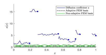
To obtain pathwise approximations of the samples , we use non-adaptive and adaptive piecewise linear elements and compare both approaches. In addition, we combine each discretization method with regular and bootstrapping multilevel Monte Carlo sampling, so in total we compare four different algorithms. The adaptive triangulation is based on each sampled partition as described in Section 4, see Fig. 1 and 3. In the graphs below, we plot the RMSE of the adaptive algorithms against the inverse estimated refinement size , for the non-adaptive algorithms this corresponds to the (deterministic) parameters . The entries of the stiffness matrix are approximated by the midpoint rule, which ensures a pathwise error of order on each simplex . To ensure that this is sufficiently precise, we repeated our experiments with a five-point Gauss-Legendre quadrature, which did not entail significant changes. In the multilevel Monte Carlo algorithm, the non-adaptive triangulations are generated with refinement , whereas we set the same threshold as maximum refinement size in the adaptive algorithm. As realized and maximal values of may differ significantly, we set for and choose the number of samples as with for . The same error equilibration is used for the non-adaptive method, only with replaced by . To subtract samples and in the MLMC estimator and add samples of the same refinement level (but on possibly different stochastic triangulations), we prolong the samples onto a reference grid with refinement size . We consider the test cases with and use with , as a reference estimate for . The RMSE is then estimated by averaging samples of the error for . To calculate the RMSE, we use a reference grid with equally spaced points in , thus the error stemming from the interpolation\prolongation may be neglected.
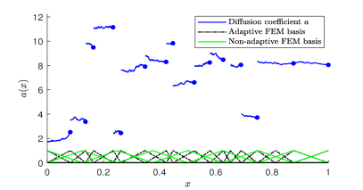
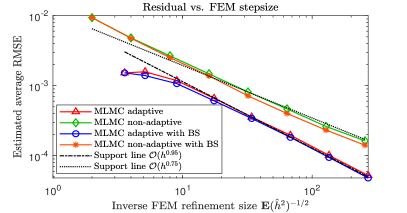
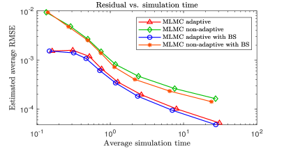
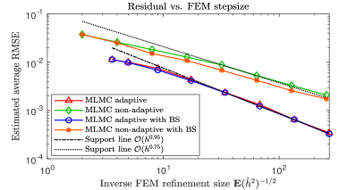
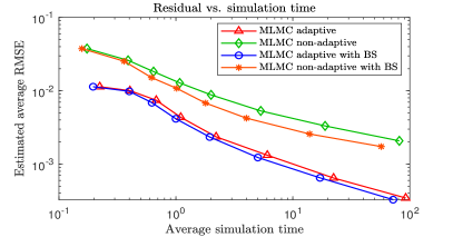
As our first numerical example, we use the Brownian motion covariance operator and i.i.d uniformly distributed jump heights , hence the sampling error is equal to zero on every level and may be omitted for this scenario. A sample of the corresponding diffusion coefficient with illustrated adaptive and non-adaptive FEM-basis is given in Fig. 1. Fig. 2 indicates that the adaptive algorithm converges considerably faster than the estimator with non-adaptive FEM basis. Asymptotically, we see that both adaptive RMSE curves decay with rate nearly one, whereas the non-adaptive methods only show a rate of . One sees that the adaptive multilevel Monte Carlo estimator also has a better time-to-error ratio, so it is possible to reduce the RMSE significantly using a little more computational effort to adjust the FEM basis in each sample. Surprisingly there is little difference in the convergence speed whether or not we use a bootstrapping algorithm combined with adaptive resp. non-adaptive FEM. Here one would expect at least a slightly higher RMSE of the bootstrapping algorithms, but in this example, the error of both bootstrapping estimators is even lower compared to their non-bootstrapping alternatives. Naturally, bootstrapping decreases computational time (see Fig. 2).
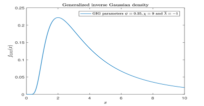
In the next example, we consider the squared exponential covariance operator and a more involved distribution of jump heights, where sampling is rather expensive and may not be realized in a straightforward manner. The jump heights now follow a continuous generalized inverse Gaussian (GIG) distribution with density
and parameters , , where is the modified Bessel function of the second kind with degrees of freedom, see [10, 11]. As shown in [6], sampling this distribution by Acceptance-Rejection is possible, but expensive when , since the vast majority of outcomes has to be rejected. We rather generate approximations of by a Fourier inversion technique such that for a given . For details on the Fourier inversion algorithm, the sampling of GIG distributions and the corresponding error bounds we refer to [13]. The GIG parameters are set as and , the resulting density and a sample of the diffusion coefficient are given in Fig. 3.
The error curves show a similar behavior compared to the first example, with asymptotic error rates of resp. for the adaptive resp. non-adaptive algorithms, see Fig. 4. Again, bootstrapping tends to produce a slightly lower RMSE. The expensive sampling from the GIG distribution causes increased computational times, which entails that the bootstrapping is even more favorable in a setting with a rather challenging jump height distributions.
The Gaussian random field with the Brownian motion covariance operator is almost surely not differentiable in a.e. , but only Hölder continuous. In addition, the covariance of the random variables and , where is given by the kernel function . For a fixed distance between and , this implies that the correlation in the random field increases as one moves to the right boundary of the domain. In some applications, however, one might instead want a random field with stationary correlation structure and/or more spatial regularity. This can be achieved with the introduced jump-diffusion coefficient by using, for instance, or another Matérn class covariance operator. These covariance operators generate random stationary correlated random fields and also increase the regularity of in . It is further possible to vary the position and magnitude of the discontinuities of to model certain desirable characteristics of the diffusion. For example, one could enforce only one jump per sample which is concentrated in some small neighborhood located around a single point in . The corresponding jump heights on each partition may then also be chosen concentrated around certain values to model, for instance, transitions in heterogeneous or fractured media.
6.2 Numerical results in 2D
In the two-dimensional setting, we work on the domain , with homogeneous Dirichlet or mixed Neumann-Dirichlet boundary conditions and we assume that the deterministic part of the drift coefficient is zero (). The Gaussian part of is given by the Karhunen-Loève expansion with spectral basis given by
with correlation length and total variance . This basis is related to the two-dimensional heat kernel
in the sense that it solves the associated integral equation for :
with the boundary condition on , see [27]. Compared with a Gaussian field generated by a squared exponential covariance operator, this field shows a very similar behavior, except that it is zero on the boundary. It, further, has the advantage, that all expressions are available in closed form and we forgo the numerical approximation of the eigenbasis. For all experiments in this section we use the parameters and . As before, we consider a log-Gaussian random field, meaning . To illustrate the flexibility of a jump-diffusion coefficient as in Def. 3.1, we vary the random partitioning of for each example and give a detailed description below. Again, we approximate the entries of the stiffness matrix by the midpoint rule on each simplex . To ensure that this is sufficient, we also tested a four-point Gauss-Legendre quadrature rule for triangular domains, which did not change the outcomes significantly. As in the previous subsection, we prolong linearly on a fixed grid to add and subtract the generated samples of the multilevel Monte Carlo estimator. The reference grid for the RMSE consists of equally spaced points in the domain , which yields a negligible interpolation error. The multilevel approximation parameters are identical to the 1D example, except that and we now calculate the reference solution on level to estimate the RMSE (by averaging independent multilevel Monte Carlo estimations) up to level or , depending on the example. All RMSE curves are plotted against the inverse estimated refinement on the abscissa.
In the first 2D example, the random partitions of are generated by random lines through the domain. More precisely, we sample independent Poisson random variables and a total of independent -distributed random variables . The first uniform random variables represent the jump positions on , the second set are the positions of the discontinuities on the opposing axis in . We connect opposing points in ascending order by straight lines to obtain a vertical random partition of . Analogously, the horizontal splitting is achieved by distributing and connecting the remaining uniform random variables on the sets and . As we obtain an average of partition elements of uniformly distributed size and location, may be set as in this example, where is the Lebesgue measure on .
To each of the random quadrangles we assign a jump height , where the sequence is i.i.d. -distributed. This specific structure of may be used, for example, to model stationary flows through heterogeneous media, where the hydraulic conductivity varies on sub-domains of the medium.
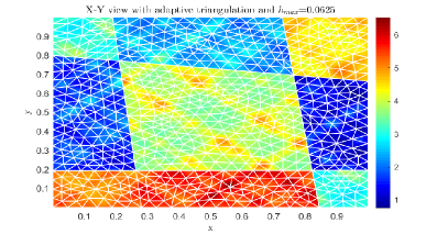
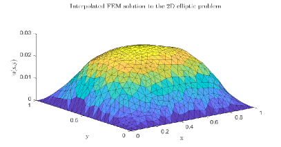
We assume homogeneous Dirichlet-boundary conditions on and as source term. A sample of the diffusion coefficient and the FEM approximation is given in Fig. 5. Compared to a solution with constant coefficient, the influence of the discontinuous diffusion is clearly visible in the contour of the approximated solution.
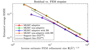
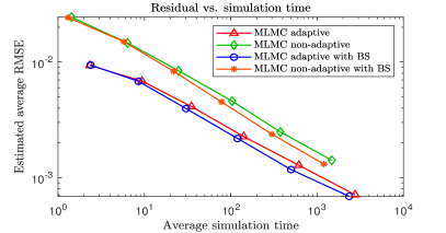
Fig. 6 shows that the adaptive multilevel Monte Carlo and non-adaptive multilevel Monte Carlo algorithm perform quite similar, where the asymptotic error rate of the nonadaptive methods is slightly lower with . Compared to that, we recover a convergence rate of and lower absolute errors for the adaptive method. In both cases, bootstrapping and normal multilevel Monte Carlo sampling produces almost identical errors which results in the best time-to-error ratio of the adaptive bootstrap multilevel Monte Carlo estimator, see Fig. 6.
In the second 2D example, we aim to mimic the structure of a fractured porous medium. To this end, we set and sample accordingly uniformly distributed random points on the domain . Then, for each point , a random length with distribution is generated. We sample, further, five random angles with uniform distribution on the set . We define as the center of a line with length rotated by , where three of the five lines are orientated horizontally and the remaining two lines are vertical. Finally, the line segments outside of are removed and each random line is assigned a positive preset width of , which results in a ”trench structure” of the diffusion coefficient as depicted in Fig. 7. On the trenches, we set the jump height to , while the jump heights on the remaining quadrangles of the partition is set to . Fixing the jump heights captures increasing permeability in the cracks of a certain medium, the Gaussian field still accounts for some uncertainty within each partition element of the domain. The source function is given as . We split by and and impose the (pathwise) mixed Dirichlet-Neumann boundary conditions
| (6.1) |
for each . A sample of the approximated solution is displayed in Fig. 7.
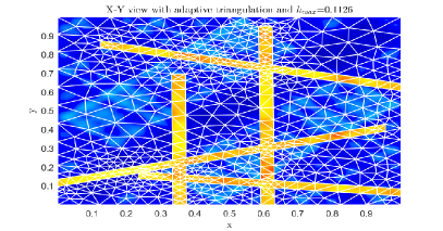
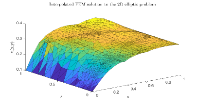
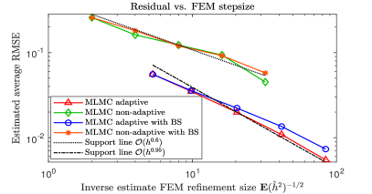
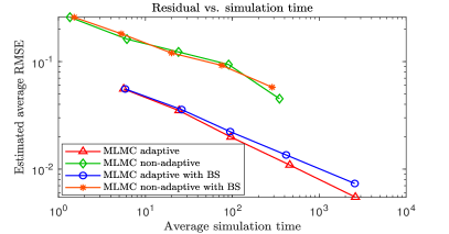
Compared to the first 2D example, there is now a larger gap between the RMSE curves of the adaptive and non-adaptive estimators, see Fig. 8. The asymptotic rate for the error is again close to order one for both adaptive methods, while we obtain for the non-adaptive algorithms. This is possibly due to the higher magnitude of the discontinuities in the diffusion coefficient compared to the first example. Bootstrapping now leads to a higher RMSE in each algorithm and this effect is more pronounced in the adaptive setting. Asymptotically, the rates of both bootstrapping estimators remain comparable to standard multilevel Monte Carlo. An adaptive triangulation for samples of this particular diffusion coefficient often entails very fine meshes, even if the desired maximum diameter of each triangle is comparably high, as Fig. 7 and Fig. 8 illustrate. Due to this increase in complexity when using adaptive FEM, the simulation times for the respective estimators are now considerably longer as in the previous scenario, see Fig. 8. Nevertheless, the adaptive methods still have significantly better time-to-error ratios, but now the standard adaptive method outperforms the corresponding bootstrapping estimator.
As a last 2D example, we discuss a medium with inclusions. To this end, we sample a discrete uniformly-distributed random variable where and define . Scaling and restricting the Lebesgue measure on means that we now draw -many uniformly distributed points within the the sub-domain . To each of this points we assign a circle of random radius. The radii are -distributed. On each circle we assign a jump height of 1, while this parameter is set to outside of the circles. We assume the same Neumann–Dirichlet boundary conditions as in our second 2D-example (see Eq. (6.1)) and as a source term we set . A sample of this jump-diffusion coefficient with corresponding FEM solution is shown in Fig. 9.
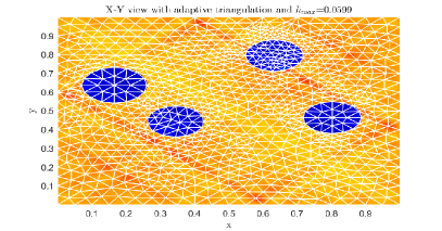
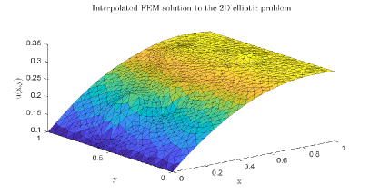
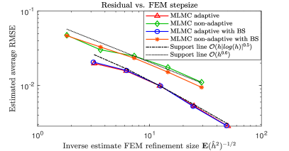
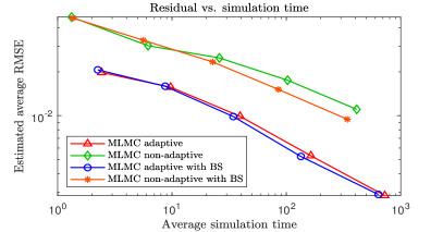
As Fig. 10 indicates, we obtain a similar behavior of convergence as in the previous example: The RMSE of the adaptive estimators is again significantly lower on all levels and the non-adaptive has again an asymptotic RMSE of order . For the adaptive methods, we obtain log-linear error decay of order . This corresponds to the expected pathwise rate for an adaptive FEM solution of this diffusion problem, as the discontinuities have -boundaries. Bootstrapping slightly reduces the RMSE of the non-adaptive method, but has little effect on the adaptive multilevel Monte Carlo estimator. The computational complexity of this scenario is comparable to the heterogeneous media example and thus significantly lower as in case of the fractured porous medium. Finally, the adaptive algorithms again attain better time-to-error with the bootstrapping estimator slightly outperforming the standard adaptive method, see Fig. 10.
Acknowledgments
The research leading to these results has received funding from the German Research Foundation (DFG) as part of the Cluster of Excellence in Simulation Technology (EXC 310/2) at the University of Stuttgart and by the Juniorprofessorship program of Baden–Württemberg, and it is gratefully acknowledged. The authors would like to thank two anonymous referees for their remarks which led to a significant improvement of the manuscript.
References
- [1] A. Abdulle, A. Barth, and C. Schwab, Multilevel Monte Carlo methods for stochastic elliptic multiscale PDEs, Multiscale Modeling & Simulation, 11 (2013), pp. 1033–1070.
- [2] R. J. Adler and J. E. Taylor, Random fields and geometry, Springer Science & Business Media, 2009.
- [3] A. Alexanderian, A brief note on the Karhunen-Loève expansion, arXiv preprint, arXiv:1509.07526, (2015).
- [4] D. Applebaum, Lévy Processes and Stochastic Calculus, Cambridge university press, 2009.
- [5] S. Asmussen and P. W. Glynn, Stochastic Simulation: Algorithms and Analysis, vol. 57, Springer Science & Business Media, 2007.
- [6] A. Atkinson, The simulation of generalized inverse Gaussian and hyperbolic random variables, SIAM Journal on Scientific and Statistical Computing, 3 (1982), pp. 502–515.
- [7] I. Babuška, The finite element method for elliptic equations with discontinuous coefficients, Computing, 5 (1970), pp. 207–213.
- [8] I. Babuška, F. Nobile, and R. Tempone, A stochastic collocation method for elliptic partial differential equations with random input data, SIAM J. Numer. Anal., 45 (2007), pp. 1005–1034 (electronic), https://doi.org/10.1137/050645142, http://dx.doi.org/10.1137/050645142.
- [9] I. Babuška, R. Tempone, and G. E. Zouraris, Galerkin finite element approximations of stochastic elliptic partial differential equations, SIAM J. Numer. Anal., 42 (2004), pp. 800–825 (electronic), https://doi.org/10.1137/S0036142902418680, http://dx.doi.org/10.1137/S0036142902418680.
- [10] O. E. Barndorff-Nielsen, Hyperbolic distributions and distributions on hyperbolae, Scandinavian Journal of Statistics, 5 (1978), pp. 151–157, http://www.jstor.org/stable/4615705.
- [11] O. E. Barndorff-Nielsen and C. Halgreen, Infinite divisibility of the hyperbolic and generalized inverse Gaussian distributions, Zeitschrift für Wahrscheinlichkeitstheorie und Verwandte Gebiete, 38, pp. 309–311, https://doi.org/10.1007/BF00533162, http://dx.doi.org/10.1007/BF00533162.
- [12] A. Barth, C. Schwab, and N. Zollinger, Multi-level Monte Carlo Finite Element method for elliptic PDEs with stochastic coefficients, Numerische Mathematik, 119 (2011), pp. 123–161.
- [13] A. Barth and A. Stein, Approximation and simulation of infinite-dimensional lévy processes, Stochastics and Partial Differential Equations: Analysis and Computations, (2016), pp. 1–49.
- [14] F. B. Belgacem, The mortar finite element method with Lagrange multipliers, Numerische Mathematik, 84 (1999), pp. 173–197.
- [15] C. Bernardi, Y. Maday, and F. Rapetti, Basics and some applications of the mortar element method, GAMM-Mitteilungen, 28 (2005), pp. 97–123.
- [16] J. Charrier, Strong and weak error estimates for elliptic partial differential equations with random coefficients, SIAM Journal on numerical analysis, 50 (2012), pp. 216–246.
- [17] J. Charrier, R. Scheichl, and A. L. Teckentrup, Finite element error analysis of elliptic PDEs with random coefficients and its application to multilevel Monte Carlo methods, SIAM Journal on Numerical Analysis, 51 (2013), pp. 322–352.
- [18] Z. Chen and J. Zou, Finite element methods and their convergence for elliptic and parabolic interface problems, Numerische Mathematik, 79 (1998), pp. 175–202.
- [19] K. A. Cliffe, M. B. Giles, R. Scheichl, and A. L. Teckentrup, Multilevel Monte Carlo methods and applications to elliptic PDEs with random coefficients, Comput. Vis. Sci., 14 (2011), pp. 3–15, https://doi.org/10.1007/s00791-011-0160-x, http://dx.doi.org/10.1007/s00791-011-0160-x.
- [20] A. Cohen, R. DeVore, and C. Schwab, Analytic regularity and polynomial approximation of parametric and stochastic elliptic PDEs, J. Analysis and Applications, 9 (2011), pp. 11–47, https://doi.org/10.1142/S0219530511001728.
- [21] G. Da Prato and J. Zabczyk, Stochastic Equations in Infinite Dimensions, Cambridge university press, second ed., 2014.
- [22] Z. Ding, A proof of the trace theorem of Sobolev spaces on Lipschitz domains, Proceedings of the American Mathematical Society, 124 (1996), pp. 591–600.
- [23] O. G. Ernst, C. E. Powell, D. J. Silvester, and E. Ullmann, Efficient solvers for a linear stochastic Galerkin mixed formulation of diffusion problems with random data, SIAM Journal on Scientific Computing, 31 (2009), pp. 1424–1447.
- [24] L. Evans, Partial Differential Equations, Graduate studies in mathematics, American Mathematical Society, 2010, https://books.google.de/books?id=Xnu0o_EJrCQC.
- [25] P. Frauenfelder, C. Schwab, and R. A. Todor, Finite elements for elliptic problems with stochastic coefficients, Computer methods in applied mechanics and engineering, 194 (2005), pp. 205–228.
- [26] M. B. Giles, Multilevel Monte Carlo path simulation, Operations Research, 56 (2008), pp. 607–617, http://www.jstor.org/stable/25147215.
- [27] D. S. Grebenkov and B.-T. Nguyen, Geometrical structure of Laplacian eigenfunctions, SIAM Review, 55 (2013), pp. 601–667, https://doi.org/10.1137/120880173, https://doi.org/10.1137/120880173, https://arxiv.org/abs/https://doi.org/10.1137/120880173.
- [28] W. Hackbusch, Elliptic Differential Equations: Theory and Numerical Treatment, Springer, Berlin; Heidelberg [u.a.], 2. softcover print. ed., 2017.
- [29] S. Heinrich, Multilevel Monte Carlo methods, Third International Conference on Large Scale Scientific Computing, 1 (2001), pp. 58–67.
- [30] H. Hoel, E. Von Schwerin, A. Szepessy, and R. Tempone, Adaptive multilevel Monte Carlo simulation, in Numerical Analysis of Multiscale Computations, Springer, 2012, pp. 217–234.
- [31] J. Li, X. Wang, and K. Zhang, Multi-level Monte Carlo weak Galerkin method for elliptic equations with stochastic jump coefficients, Applied Mathematics and Computation, 275 (2016), pp. 181–194.
- [32] W. V. Li and Q.-M. Shao, Gaussian processes: inequalities, small ball probabilities and applications, Handbook of Statistics, 19 (2001), pp. 533–597.
- [33] F. Nobile, R. Tempone, and C. G. Webster, A sparse grid stochastic collocation method for partial differential equations with random input data, SIAM J. Numer. Anal., 46 (2008), pp. 2309–2345, https://doi.org/10.1137/060663660, http://dx.doi.org/10.1137/060663660.
- [34] B. Peherstorfer, K. Willcox, and M. Gunzburger, Optimal model management for multifidelity Monte Carlo estimation, SIAM Journal on Scientific Computing, 38 (2016), pp. A3163–A3194, https://doi.org/10.1137/15M1046472, https://doi.org/10.1137/15M1046472, https://arxiv.org/abs/https://doi.org/10.1137/15M1046472.
- [35] M. Petzoldt, A posteriori error estimators for elliptic equations with discontinuous coefficients, Advances in Computational Mathematics, 16 (2002), pp. 47–75.
- [36] C. E. Rasmussen and C. K. I. Williams, Gaussian processes for machine learning, Adaptive Computation and Machine Learning, MIT Press, Cambridge, MA, 2006.
- [37] C. Schwab and C. J. Gittelson, Sparse tensor discretizations of high-dimensional parametric and stochastic PDEs, Acta Numerica, 20 (2011), pp. 291–467, https://doi.org/10.1017/S0962492911000055.
- [38] A. L. Teckentrup, R. Scheichl, M. B. Giles, and E. Ullmann, Further analysis of multilevel Monte Carlo methods for elliptic PDEs with random coefficients, Numerische Mathematik, 125 (2013), pp. 569–600, https://doi.org/10.1007/s00211-013-0546-4, http://dx.doi.org/10.1007/s00211-013-0546-4.
- [39] D. Zhang and Q. Kang, Pore scale simulation of solute transport in fractured porous media, Geophysical Research Letters, 31 (2004), https://doi.org/10.1029/2004GL019886, http://dx.doi.org/10.1029/2004GL019886. L12504.
- [40] D. Zhang and Z. Lu, An efficient, high-order perturbation approach for flow in random porous media via Karhunen–Loève and polynomial expansions, Journal of Computational Physics, 194 (2004), pp. 773–794, https://doi.org/http://dx.doi.org/10.1016/j.jcp.2003.09.015, http://www.sciencedirect.com/science/article/pii/S0021999103005072.