Stock market as temporal network

Abstract

Financial networks have become extremely useful in characterizing the structure of complex financial systems. Meanwhile, the time evolution property of the stock markets can be described by temporal networks. We utilize the temporal network framework to characterize the time-evolving correlation-based networks of stock markets. The market instability can be detected by the evolution of the topology structure of the financial networks. We employ the temporal centrality as a portfolio selection tool. Those portfolios, which are composed of peripheral stocks with low temporal centrality scores, have consistently better performance under different portfolio optimization schemes, suggesting that the temporal centrality measure can be used as new portfolio optimization and risk management tools. Our results reveal the importance of the temporal attributes of the stock markets, which should be taken serious consideration in real life applications.

1 Introduction

The correlation-based network has become an effective tool to investigate the correlation between complex financial systems[1, 2]. Different methods have been proposed to probe the complex correlation structure of financial system including the threshold method, the minimum spanning tree(MST)[3], the planar maximumly filtered graph(PMFG)[4] and a strand of other methods[5, 6, 7, 8, 9, 10, 11]. The common aim of all correlation-based networks is seeking for a sparse representation of the high dimensional correlation matrix of the complex financial system. Unlike other eigenvector-based methods(e.g., the principal component analysis) which decompose the variance of the system into a few dimensions, the correlation-based methods directly map the dense correlation matrix into sparse representation. The easy implementations and straightforward interpretations of those methods make them quite popular in complex system analysis, especially for complex financial systems. Recently, the correlation-based network has been used for portfolio selection in which some risk diversified portfolios are constructed based on a hybrid centrality measure of the MST and PMFG networks of the stock return time series[12]. It is well known that the financial system has its own temporal properties which makes it extremely hard or even impossible to forecast. Thus if we want to construct our portfolio in a proper way, we have to consider the temporal attribute of the financial system.

In this work, we analyze the correlation-based networks of stock markets by using the temporal network paradigm. Specifically we have analyzed the temporal evolution of three major stock markets of the world, namely, the US, the UK and China. Based on a centrality measure of temporal network, we also construct some portfolios that consistently perform the best under two portfolio optimization schemes. Our work is the first research that incorporates the temporal network methods into the study of complex financial system. The temporal evolution of the topological structures can be used to access the information of market instability. The effectiveness of the temporal centrality measure in portfolio selection depicts the importance of the temporal structure for the analysis of stock market. The remainder of the paper is organized as follows: Section 2 gives the data description and the methodology we use through the paper. Section 3 presents the main results of the paper including the topology analysis of the stock markets and the application to the portfolio optimization problems. Section 4 is the conclusion.

2 Data and methodology

2.1 Data

Our data sets include the daily returns of the constitute stocks of three major indexes in the world: S&P 500 (the US), FTSE 350 (the UK) and SSE 380 (China). After removing those stocks with very small sample size, we still have 401, 264, and 295 stocks for the three markets respectively. In the S&P 500 dataset, each stock includes 4025 daily returns from 4 January 1999 to 31 December 2014. The FTSE 350 stocks include 3000 daily returns in the period between 10 October 2005 and 26 April 2017. The SSE 380 stocks consist of 2700 daily returns from 21 May 2004 to 19 November 2014.

2.2 Cross-correlation between stocks

We adopt the logarithm return defined as

$$r_{i}(t)=\mathrm{ln}p_{i}(t+1)-\mathrm{ln}p_{i}(t),$$ (1)

where $p_{i}(t)$ is the adjusted closure price of stock $i$ at time $t$. We then compute the cross-correlation coefficients between any pair of return time series at time $t$ by using the past return records sampled from a moving window with length $\Delta$. We then calculate the similarity between stocks $i$ and $j$ at time $t$ with the traditional Pearson correlation coefficient,

$$\rho_{ij}^{t,\Delta}=\frac{\langle R_{i}^{t}R_{j}^{t}\rangle-\langle R_{i}^{t}\rangle\langle R_{j}^{t}\rangle}{\sqrt{\left[\langle R_{i}^{t^{2}}\rangle-\langle R_{i}^{t}\rangle^{2}\right]\left[\langle R_{j}^{t^{2}}\rangle-\langle R_{j}^{t}\rangle^{2}\right]}},$$ (2)

where $\Delta$ is the moving window length, and $\langle\ldots\rangle$ is the sample mean over co-trading days of stocks $i$ and $j$ in the logarithm return series vector $R_{i}^{t}=\{r_{i}(t)\}$ and $R_{j}^{t}=\{r_{j}(t)\}$. We obtain an $N\times N$ matrix $\mathrm{\textbf{C}}^{t,\Delta}$ at time $t$ with estimation windows $\Delta$ days, and $N$ is the number of stocks. The entries of $\mathrm{\textbf{C}}^{t,\Delta}$ are cross-correlation coefficients $\rho_{ij}^{t,\Delta}$ between all pairs of stocks. The moving window widths are $\Delta=500$ days for S&P 500 and $\Delta=300$ days for both FTSE 350 and SSE 380. The moving window widths are chosen to make the correlation matrix non-singular(with $\Delta\geq N$). With moving window width $\Delta$, we shift the moving window with 25 days step, thus we obtain a strand of correlation matrices for three markets. Finally we have 142 correlation matrices for S&P 500, 109 correlation matrices for FTSE 350 and 97 correlation matrices for SSE 380 respectively.

2.3 PMFG network of stock market

Since the dense representation given by the cross-correlation matrix will induce lots of redundant information, thus it is very hard to discriminate the important information from noise. Here we employ the the planar maximally filtered graph(PMFG) method [4] to construct sparse networks based on correlation matrices $\mathrm{\textbf{C}^{t,\Delta}}$. The algorithm is implemented as follows,
(i) Sort all of the $\rho_{ij}^{t,\Delta}$ in descending order in an ordered list $l_{sort}$.
(ii) Add an edge between nodes $i$ and $j$ according to the order in $l_{sort}$ if and only if the graph remains planar after the edge is added.
(iii) Repeat the second step until all elements in $l_{sort}$ are used up.

Finally a planar graph $G^{t,\Delta}$ is formed with $N_{e}=3(N-2)$ edges. It has been addressed in Ref.[4] that the PMFG not only keeps the hierarchical organization of the MST but also induces cliques. We calculate such basic topological quantities as the clustering coefficient $C$ and the shortest-path length $L$[13]. A heterogeneity index $\gamma$ [14] is also used to measure the heterogeneity of PMFGs which is defined by

$$\gamma=\frac{N-2\sum\limits_{ij\in{\{e\}}}(k_{i}k_{j})^{-1/2}}{N-2\sqrt{N-1}},$$ (3)

where $k_{i}$ and $k_{j}$ are the degrees of nodes $i$ and $j$ connected by edge $\{e_{ij}\}$. We also utilize the Jaccard index[15] $J$ to show the variability of the network structure form $t$ to $t+1$. The Jaccard index $J_{G_{1}G_{2}}$ between networks $G_{1}$ and $G_{2}$ is defined as

$$J_{G_{1},G_{2}}=\frac{E_{G_{1}}\cap E_{G_{2}}}{E_{G_{1}}\cup E_{G_{2}}},$$

where $E_{G_{1}}$ and $E_{G_{2}}$ are the edges of networks $G_{1}$ and $G_{2}$, respectively.

2.4 Supra-Evolution matrix for temporal stock network

We use the moving window technique to construct time-varying correlation matrices and PMFG networks. Considering the temporal properties of the stock market, it is impossible to fully describe the whole system with a single adjacency matrix. Previous studies try to resolve this problem by aggregating temporal networks into a static network[16]. However, the obvious drawback of this approach is that the information about the time evolution of the system is missing. Very recently, the research about temporal and multilayer network have become the new frontier of network science[17, 18, 19]. The mathematical formulation of the multilayer network provide us a possible way to describe the temporal network structure in a unified way. Since the only difference between temporal network and multilayer network is the direction of the coupling between each layer. Thus we treat the temporal stock network as a special case of multilayer network and analyze its properties based on the supra-adjacency matrix[19, 20] Actually the supra-adjacency matrix concept has already been used to describe the temporal networks in Ref.[19, 21].

Here a series of PMFG networks can be described as $G^{t}=(V,E)^{t},t\in(1\ldots T)$. The adjacency matrix of PMFG $G^{t}$ at time $t$ is denoted by $A^{t}$. For the temporal stock network, the network size $N$ of each time slice is fixed. The coupling matrix between different time layers is an $N\times N$ dimension matrix $W_{t_{a}t_{b}}$. Then the supra-adjacency matrix with dimension $NT\times NT$ can be written as,

$$\textbf{A}=\left(\begin{array}[]{cccc}A^{1}&W_{12}&\cdots&W_{1T}\\ W_{12}&A^{2}&\cdots&W_{2T}\\ \vdots&\vdots&\ddots&\vdots\\ W_{T1}&W_{T2}&\cdots&A^{T}\end{array}\right),$$

here A is the supra-adjacency matrix with bidirectional coupling. However, for temporal network the coupling is directional. So the upper triangle of the supra-adjacency matrix should be zero. As described in Ref.[21], the supra-adjacency is named as supra-evolution matrix with a time directional coupling. The adjacency matrix $A^{t}$ is easy to obtain. The big challenge here is how to determine the coupling matrix $W_{t_{a}t_{b}}$. The temporal stock network is different from the real multilayer network for which the coupling between each layer is well defined. Thus we employ the time series analysis method to model the evolution of the stock network. The coupling between two networks at successive time slices can be obtained from time series modeling. We use the autoregressive moving average model($\mathrm{ARMA}$) to fit the correlation strength time series of each stock. Considering the non-stationarity of the correlation strength time series, before the $\mathrm{ARMA}$ model is applied, we need to difference those time series to make them meet the stationary requirements meaning that the actual correlation strength time series can be fitted with the $\mathrm{ARIMA}(p,d,q)$ with differencing order $d$. The $\mathrm{ARMA}(p,q)$ model is described as[22]:

$$s_{i,t}=\phi_{i,1}s_{i,t-1}+\phi_{i,2}s_{i,t-2}+\ldots+\phi_{i,p}s_{i,t-p}$$

$$+e_{t}-\theta_{i,1}e_{t-1}-\theta_{i,2}e_{t-2}-\ldots-\theta_{i,q}e_{t,q},$$

where $s_{i,t}=\sum\limits_{j=1}^{N}\rho_{i,j}^{t}$ is the correlation strength of stock $i$ at time $t$. $e_{t}$ is Gaussian noise. Whist $\Phi_{i,p}=(\phi_{i,1},\phi_{i,2},\ldots,\phi_{i,p})$ and $\Theta_{i,q}=(\theta_{i,1},\theta_{i,2},\ldots,\theta_{i,q})$ are the model parameters(AR and MA parts) with model orders $p$ and $q$.

The autoregressive parameters $\Phi_{i,p}$ specify that the correlation strength $s_{i,t}$ of node $i$ depends linearly on its own previous $p\mathrm{th}$ values. Thus the coupling matrix $W_{t_{a},t_{b}}$ for $t_{a}>t_{b}$ can be written as

$$W_{2,1}=\ldots=W_{t,t-1}=(\phi_{i,1})_{N\times N}=\left(\begin{array}[]{cccc}\phi_{1,1}&0&\cdots&0\\ 0&\phi_{2,1}&\cdots&0\\ \vdots&\vdots&\ddots&\vdots\\ 0&0&\cdots&\phi_{N,1}\end{array}\right)$$

$$W_{t,t-2} =(\phi_{i,2})_{N\times N},i=1,2,\ldots,N,$$

$$\ldots$$

$$W_{t,t-l} =(\phi_{i,l})_{N\times N},i=1,2,\ldots,N.$$

While for $t_{a}<t_{b}$, we set $W_{t_{a},t_{b}}$ to zero matrix. So the supra-evolution matrix is a lower triangle block matrix

$$\textbf{A}=\left(\begin{array}[]{cccc}A^{1}&0&\cdots&0\\ W_{2,1}&A^{2}&\cdots&0\\ \vdots&\vdots&\ddots&\vdots\\ W_{T,1}&W_{T,2}&\cdots&A^{T}\end{array}\right).$$

With the supra-evolution matrix, we can define some centrality measure to quantify the importance of different stocks. Many centrality measures are based on the element of leading eigenvector corresponds to the largest eigenvalue of different matrices(e.g., adjacency matrix). The temporal centrality can be defined by the largest eigenvalue and corresponding eigenvector of the supra-evolution matrix, i.e.,

$$\mathrm{\textbf{A}}\boldsymbol{\nu_{1}}=\lambda_{1}\boldsymbol{\nu_{1}},$$ (4)

where $\boldsymbol{\nu_{1}}$ is the eigenvector corresponding to the largest eigenvalue $\lambda_{1}$ with dimension $NT\times 1$, $\boldsymbol{\nu_{1}}=(\nu_{i}^{t})_{NT\times 1},i=1,2,\ldots,N;t=1,2,\ldots,T$. The element $\nu_{i}^{t}$ represents the centrality value of node $i$ at time $t$. Thus for node $i$ in temporal stock network, the eigenvector centrality $c_{i}$ can be defined as the summation of the value of $\nu_{i}^{t}$ in different time slices, namely,

$$c_{i}=\sum\limits_{t=1}^{T}\nu_{i}^{t},i=1,2,\ldots,N.$$ (5)

3 Results and Application

3.1 Topology analysis of temporal stock networks

Figure 1: The time evolution of the topological quantities of the PMFG networks for three markets. The first column is the topological quantities of the PMFG networks for S&P 500 constituent stocks. The second column is the topological quantities of the PMFG networks for the FTSE 350 constituent stocks. The third column is the topological quantities of the PMFG networks for the SSE 380 constituent stocks. The first row is the clustering coefficient $C$ for three markets. The second row is the shortest path length $L$ for three markets. The third row is the heterogeneity index $\gamma$ for three markets. The last row is the Jaccard index $J$ for three markets.

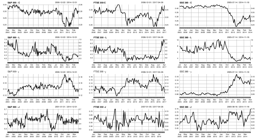
In Fig.1, we show the time evolution of the topological parameters of PMFG networks for the three markets. For the US stock market, the topology structures of the PMFG networks respond to the 2008 sub-prime crisis during which the Jaccard index decreased dramatically. It means the market suffered from extremely unstable period with drastic structure variation. For the UK market, during the European debt crisis, the clustering coefficient $C$ and shortest path length $L$ both decreased. The heterogeneity index $H$ of the PMFG network increase significantly during the crisis. The reaction of the correlation-based networks during financial crisis has been systematically investigated[23, 24, 25, 26, 27, 28, 29]. Here we find that the heterogeneity index of China stock market is apparently small before 2012 with higher clustering coefficient $C$ and longer shortest path length $L$. It is known that the heterogeneity value $H$ of the scale-free network is 0.11. The western markets are more heterogeneous than the scale-free network and they are considerably more heterogeneous than China market. The homogeneous structure of Chinese market before 2012 indicates that the Chinese market has totally different structure compare to the western markets. During the period between 2011 and 2014, the Chinese stock market suffered from a long term bear market. The market heterogeneity increased dramatically during that period. This means that the market try to get rid of the domination of the index or the market trend, which maybe resulted from the risk diversification of the investors or the market becoming mature. Although we can obtain some information from the variation of those topological parameters, those quantities suffer from the very unstable market states and strong noise. The evolution of those topology quantities indicate that the markets are always evolving over time. The temporal properties of the stock markets should be considered and incorporated into real life applications. In the next section, we try to utilize the temporal attributes to improve the performance of the portfolio optimization procedure.

3.2 Portfolio optimization

3.2.1 Mean-variance portfolio optimization

We first employ the PMFG networks to improve the performance of portfolio optimization under the Markowitz portfolio optimization framework[30]. There are lots of works trying to establish connections between the correlation-based networks and the portfolio optimization problems[31, 32, 33]. We now give an brief introduction about the Markowitz portfolio theory. Consider a portfolio of $m$ stocks with return $r_{i},i=1\ldots m$. The return $\Pi(t)$ of the portfolio is

$$\Pi(t)=\sum\limits_{i=1}^{m}\omega_{i}r_{i}(t),$$

where $\omega_{i}$ is the investment weight of stock $i$. $\omega_{i}$ is normalized such that $\sum\limits_{i=1}^{m}\omega_{i}=1$. The risk of the portfolio can be simply quantified by the variance of the return

$$\Omega^{2}=\sum\limits_{i=1}^{m}\sum\limits_{j=1}^{m}\omega_{i}\omega_{j}\rho_{ij}\sigma_{i}\sigma_{j},$$

here $\rho_{ij}$ is the Pearson cross-correlation between $r_{i}$ and $r_{j}$, and $\sigma_{i}$ and $\sigma_{j}$ are the standard deviations of the return time series $r_{i}$ and $r_{j}$. The optimal portfolio weights are determined via maximize the portfolio return $\Phi=\sum\limits_{t=1}^{T}\Pi(t)$ under the constraint that the risk of the portfolio equals to some fixed value $\Omega^{2}$. Maximizing $\Phi$ subject to those constraints above can be formulated as a quadratic optimization problem:

$$\omega^{T}\Sigma\omega-q*\mathrm{R}^{T}\omega,$$

where $\Sigma$ is the covariance matrix of the return time series. The parameter $q$ is the risk tolerance parameter with $q\in[0,\infty)$. Large $q$ indicates that the investors have strong tolerance to the risk which may give large expected return. Whilst, small $q$ represents that the investors are extremely risk aversion. The optimal portfolios at different risk and return levels can be presented as the efficient frontier which is a plot of the return $\Phi$ as a function of risk $\Omega^{2}$.

So far we have not illustrate how to determined the constitute stocks of a specific portfolio. As mentioned in the previous context, we use some centrality metric to choose portfolio from the PMFG networks. It has shown that the performance of the portfolio selected by using some compound centrality measures for the static PMFG networks is quite good[12, 34]. Here we try to select the portfolio guided by the temporal eigenvector centrality measure of the temporal PMFG networks for different stock markets. A portfolio constructed by using the central (peripheral) stocks is the one that consists of those higher (lower) centrality value stocks. For comparison, we also perform the portfolio optimization procedure based on aggregated networks[16]. For the aggregated network, we use the compound centrality measure from Ref.[12] to rank the stocks. In contrast, in the temporal stock networks, the stocks are ranked according to the temporal centrality given by Eq. 5. To verify the robustness of the portfolios’ performances, we performed both in sample and out of sample tests for those temporal portfolios.

Figure 2: The in sample efficient frontiers for three different stock markets. The left, center and right columns are the results for S&P 500, FTSE 350 and SSE 380 respectively. The red lines are the results for those portfolios constructed from stocks with high centrality scores(central) for both temporal(suffix -temp) and aggregated(suffix -agg) networks. The blue lines are the results for those portfolios constructed from stocks with low centrality scores(peripheral). Here the portfolio size $m=30$. We have tested the portfolio size from $m=5$ up to $m=60$, the results are consistent.

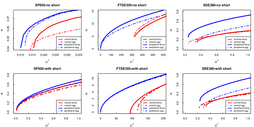
Fig. 2 shows the in sample efficient frontiers of a portfolio constructed by those stocks with 30 highest centrality and 30 lowest centrality stocks for both aggregated and temporal stock networks. Here during the in sample tests, the whole datasets(with 4205, 3000 and 2700 records for US, UK and China respectively) have been used to construct the temporal networks and the portfolio optimization is also performed with the whole datasets. The solid lines are those portfolios selected guided by the eigenvector centrality for temporal PMFG networks. The dashed lines are those portfolios for aggregated networks. The aggregated network is constructed by combining all the vertices and edges in all the time slices of temporal networks. The solid and dashed red (blue) lines are those portfolios of central(peripheral) stocks. It is very clear that the performance of the peripheral portfolios are much better than those central ones for three markets. That is exactly in line with the previous research. Meanwhile, the in sample performance of portfolios for temporal networks(solid lines) are also better than those constructed from aggregate networks(dashed lines). The overall best in sample performance comes from those portfolios constructed based on temporal networks and peripheral stocks(solid blue lines). Those portfolios have the highest return and the lowest risk compared with other portfolios.

Figure 3: The out of sample efficient frontiers of three different stock markets. The left, center and right columns are the results for SP500, FTSE350 and SSE380, respectively. The red lines are the results for those portfolios constructed from stocks with high centrality scores(central) for both temporal(suffix -temp) and aggregated(suffix -agg) networks. The blue lines are the results for those portfolios constructed from stocks with low centrality scores(peripheral). Here the portfolio size $m=30$. We have tested the portfolio size from $m=5$ up to $m=60$, the results are consistent.

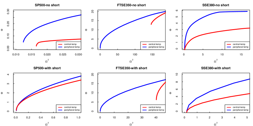
The out of sample tests are also performed to check the robustness of the temporal network portfolios. Here in Fig. 3, we perform the out of sample tests for temporal portfolios. First we use the first 3500, 1650 and 1500 data points for US, UK and China markets to construct the temporal networks. With the guidance of temporal centrality, we can construct the central and peripheral portfolios. Then the next 225 data points are used to perform the portfolio optimization procedure. The results are very similar to the in sample tests. The temporal peripheral portfolios have consistent good performance over the central portfolios. A very interesting phenomena is that the central portfolios of UK market always have very high risk for both in sample and out of sample tests. The central portfolios can not attain risks lower than some specific level even for very small risk tolerance parameter $q$. This implies that the central stocks of UK market are extremely risky which should definitely be avoided by investors. The above portfolio optimization results evidence the usefulness of temporal centrality metric. The temporal information of the correlation-based networks should be taken into consideration when dealing with time evolving systems.

3.2.2 Expected shortfall approach

Apart from the mean-variance framework, the expected shortfall($ES$) is a more modern tool of quantifying the performance of a portfolio, which is a coherent risk measure[35, 36, 37]. Let $X$ be the profit loss of a portfolio within a specified time horizon $(0,T)$ and let $\alpha=\eta\%\in(0,1)$ be some specified probability level. The expected $\eta\%$ shortfall of the portfolio can be defined as

$$ES^{\alpha}(X)=-\frac{1}{\alpha}(E[X\textbf{1}_{X\leq x^{\alpha}}]-x^{\alpha}(\mathrm{P}[X\leq x^{\alpha}]-\alpha)).$$ (6)

The $ES$ gives the expected loss incurred in the $\eta\%$ worst situations of the portfolio. It satisfies all the requirements of a risk measure. For a portfolio $\{\omega_{i},i=1,\ldots,m\}$ of $m$ stocks with return $\{r_{i},i=1,\ldots,m\}$, we want to minimize the $ES^{\alpha}$ of the portfolio under the constraint of $\sum\limits_{i=1}^{m}\omega_{i}=1$. Here we set the confidence level $\alpha=95\%$ for the expected shortfall $ES^{\alpha}$ of the portfolio and assume that the short selling is prohibited. After ranking the stocks according to the centrality scores described in the previous subsection, we choose the portfolio size $m=5,10,\ldots,55,60$, namely, $m$ central(peripheral) stocks with the largest(smallest) centrality scores.

Figure 4: The in sample expected shortfalls for three stock markets. The left, center and right columns are the results for S&P 500, FTSE 350 and SSE 380, respectively. The red(blue) lines are the expected shortfalls for the portfolios constructed by central(peripheral) stocks. The solid lines are the expected shortfalls for temporal networks. The dashed lines are those for aggregated(suffix -agg) networks and the solid liens are those for temporal(suffix -temp) networks.

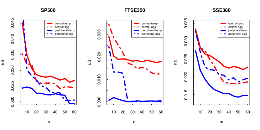
Fig .4 gives the in sample expected shortfalls for the three stock markets. The red(blue) lines represent the expected shortfalls for central(peripheral) portfolios. The solid(dashed) lines corresponds to the temporal(aggregated) networks. It is obvious that the expected shortfalls for peripheral portfolios are much smaller than the central ones. An argument has been given in Ref.[33] in which the correlation matrix can be recognized as an weighted fully connected network. There exists a negative correlation between the weights of the optimal portfolio and the network’s eigenvector centralities. The lower expected shortfalls of peripheral portfolios have verified this argument. Whilst, the temporal centrality as a portfolio selection tool performs even better than the static aggregated network centrality up to $m=60$ portfolio size.

Figure 5: The out of sample expected shortfalls for three stock markets. The left, center and right columns are the results for S&P 500, FTSE 350 and SSE 380, respectively. The red(blue) lines are the expected shortfalls for the portfolios constructed by central(peripheral) stocks.

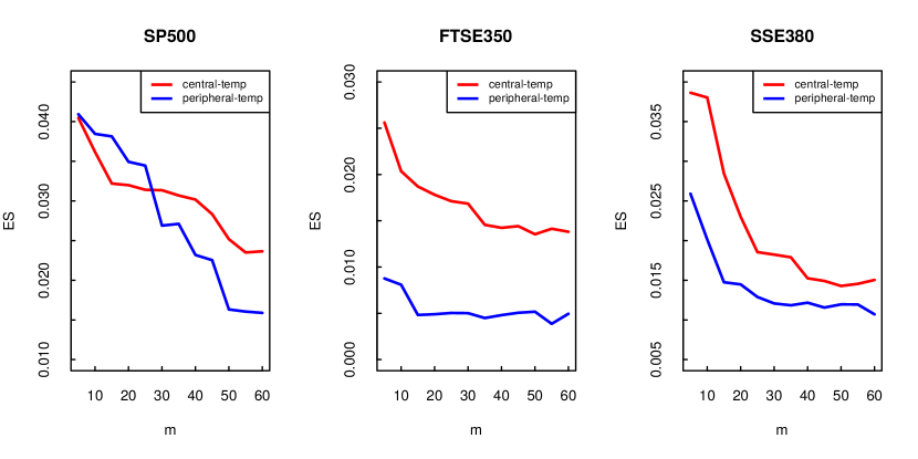
In Fig. 5, the out of sample tests are also performed for three markets. The datasets used for the out of sample tests are exactly the same as in previous subsection. Except for the temporal portfolio with size $m=5$ of the US market, the peripheral portfolios for the three markets with portfolio size up to $m=60$ all have better performances with lower expected shortfalls. We argue that the consistent good performance of the temporal portfolio rooted in the time average attribute of the temporal centrality. It can weaken the influence of large fluctuations of the market, thus it can be used to construct more robust and risk diversified portfolio[38, 39, 34].

4 Conclusion

In conclusion, we have used the temporal network scheme to analyze the temporal evolution of three major stock markets. The topology evolution of the correlation-based networks for three markets give some signals of corresponding financial turbulences in each market. With the help of temporal centrality measure, we can construct some risk diversified portfolios with high return and low risk. Under both the mean-variance and expected shortfall frameworks, the portfolios constructed with those peripheral stocks in both temporal and static centrality measures outperform those portfolios constructed with central stocks. Moreover, those peripheral portfolios selected with the guidance of temporal centrality measure performed way better than other portfolios(central portfolios and aggregated peripheral portfolios) under both mean-variance and expected shortfall evaluation scheme. The in sample and out of sample tests have verified the robustness of the temporal peripheral portfolios. This is the first study to analyze the time evolving correlation-based networks with temporal network theory. The application of temporal centrality measure on portfolio selection has revealed the importance of the temporal attributes of the correlation-based networks of stock markets. Thus it should be quite interesting to investigate the temporal structure of the correlation-based networks with other tools developed for temporal network[16]. This should be subject to future research.

5 Acknowledgment

This work is supported in part by the Programme of Introducing Talents of Discipline to Universities (Grant no. B08033), the NSFC (Grant no. 71501066), the Hunan Provincial Natural Science Foundation of China (Grant no. 2017JJ3024), and the program of China Scholarship Council (Grant no. 201606770023).

References

- [1] Gautier Marti, Frank Nielsen, Mikołaj Bińkowski, and Philippe Donnat. A review of two decades of correlations, hierarchies, networks and clustering in financial markets. arXiv, pages 1–25, 2017.
- [2] Jarosław Kwapień and Stanisław Drożdż. Physical approach to complex systems. Physics Reports, 515(3-4):115–226, jun 2012.
- [3] RN N R.N. Mantegna. Hierarchical structure in financial markets. European Physical Journal B, 197(1):193–197, 1999.
- [4] M. Tumminello, T. Aste, T. Di Matteo, and R. N. Mantegna. A tool for filtering information in complex systems. Proceedings of the National Academy of Sciences of the United States of America, 102(30):10421–10426, jul 2005.
- [5] Dror Y Kenett, Michele Tumminello, Asaf Madi, Gitit Gur-Gershgoren, Rosario N Mantegna, and Eshel Ben-Jacob. Dominating clasp of the financial sector revealed by partial correlation analysis of the stock market. PloS one, 5(12):e15032, jan 2010.
- [6] SHI-MIN CAI, YAN-BO ZHOU, TAO ZHOU, and PEI-LING ZHOU. Hierarchical Organization and Disassortative Mixing of Correlation-Based Weighted Financial Networks. International Journal of Modern Physics C, 21(03):433–441, 2010.
- [7] Ya-Chun Gao, Yong Zeng, and Shi-Min Cai. Influence network in Chinese stock market. Journal Of Statistical Mechanics-Theory And Experiment, 2015(3):1–14, 2015.
- [8] Siew Lee Gan and Maman Abdurachman Djauhari. New York Stock Exchange performance: evidence from the forest of multidimensional minimum spanning trees. Journal of Statistical Mechanics: Theory and Experiment, 12005:P12005, 2015.
- [9] Gang-Jin Wang, Chi Xie, Kaijian He, and H Eugene Stanley. Extreme risk spillover network: application to financial institutions. Quantitative Finance, 17(9):1417–1433, 2017.
- [10] Gang-Jin Wang, Chi Xie, and Shou Chen. Multiscale correlation networks analysis of the US stock market: a wavelet analysis. Journal of Economic Interaction and Coordination, 12(3):561–594, oct 2017.
- [11] Gang-Jin Wang and Chi Xie. Tail dependence structure of the foreign exchange market: A network view. Expert Systems with Applications, 46(Supplement C):164–179, 2016.
- [12] F. Pozzi, T. Di Matteo, and T. Aste. Spread of risk across financial markets: better to invest in the peripheries. Scientific Reports, 3(1):1665, 2013.
- [13] Réka Albert and Albert Laszlo Barabasi. Statistical mechanics of complex networks. Reviews of Modern Physics, 74(1):47–97, 2002.
- [14] Ernesto Estrada. Quantifying network heterogeneity. Physical Review E, 82(6):66102, 2010.
- [15] Paul Jaccard. THE DISTRIBUTION OF THE FLORA IN THE ALPINE ZONE.1. New Phytologist, 11(2):37–50, feb 1912.
- [16] Petter Holme and Jari Saramäki. Temporal networks. Physics Reports, 519(3):97–125, oct 2012.
- [17] Mikko Kivelä, Alex Arenas, Marc Barthelemy, James P. Gleeson, Yamir Moreno, and Mason A. Porter. Multilayer networks. Journal of Complex Networks, 2(3):203–271, 2014.
- [18] S. Boccaletti, G. Bianconi, R. Criado, C. I. del Genio, J. Gómez-Gardeñes, M. Romance, I. Sendiña-Nadal, Z. Wang, and M. Zanin. The structure and dynamics of multilayer networks. Physics Reports, jul 2014.
- [19] Dane Taylor, Sean A. Myers, Aaron Clauset, Mason A. Porter, and Peter J. Mucha. Eigenvector-Based Centrality Measures for Temporal Networks. MULTISCALE MODEL. SIMUL, 15(1):537–574, 2015.
- [20] Manlio De Domenico, Albert Solé-Ribalta, Emanuele Cozzo, Mikko Kivelä, Yamir Moreno, Mason A. Porter, Sergio Gómez, and Alex Arenas. Mathematical formulation of multilayer networks. Physical Review X, 3(4):1–15, 2014.
- [21] Qiangjuan Huang, Chengli Zhao, Xue Zhang, Xiaojie Wang, and Dongyun Yi. Centrality measures in temporal networks with time series analysis. EPL (Europhysics Letters), 118(3):36001, 2017.
- [22] George E P Box. Time series analysis : forecasting and control. Wiley, Hoboken, New Jersey, 5th ed. edition, 2015.
- [23] Michele Tumminello, Fabrizio Lillo, and Rosario N. Mantegna. Correlation, hierarchies, and networks in financial markets. Journal of Economic Behavior & Organization, 75(1):40–58, jul 2010.
- [24] Dong-Ming Song, Michele Tumminello, Wei-Xing Zhou, and Rosario N. Mantegna. Evolution of worldwide stock markets, correlation structure, and correlation-based graphs. Physical Review E, 84(2):026108, aug 2011.
- [25] Gang Jin Wang, Chi Xie, Yi Jun Chen, and Shou Chen. Statistical properties of the foreign exchange network at different time Scales: Evidence from detrended cross-correlation coefficient and minimum spanning tree. Entropy, 15(5):1643–1662, 2013.
- [26] Longfeng Zhao, Wei Li, and Xu Cai. Structure and dynamics of stock market in times of crisis. Physics Letters A, 380(5-6):654–666, 2016.
- [27] Ashadun Nobi, Sungmin Lee, Doo Hwan Kim, and Jae Woo Lee. Correlation and network topologies in global and local stock indices. Physics Letters A, 378(34):2482–2489, jul 2014.
- [28] Dror Y. Kenett and Shlomo Havlin. Network science: a useful tool in economics and finance. Mind and Society, 14(2):155–167, 2015.
- [29] Gang-Jin Wang and Chi Xie. Correlation structure and dynamics of international real estate securities markets: A network perspective. Physica A: Statistical Mechanics and its Applications, 424(March 2016):176–193, 2015.
- [30] Harry Markowitz. Portfolio Selection. The Journal of Finance, 7(1):77, mar 1952.
- [31] J.-P. Onnela, A. Chakraborti, K. Kaski, J. Kertesz, A. Kanto, and J. Kertész. Dynamics of market correlations: Taxonomy and portfolio analysis. Physical Review E, 68(5):056110, nov 2003.
- [32] Vincenzo Tola, Fabrizio Lillo, Mauro Gallegati, and Rosario N Mantegna. Cluster analysis for portfolio optimization. Journal of Economic Dynamics and Control, 32(1):235–258, 2008.
- [33] Gustavo Peralta and Abalfazl Zareei. A network approach to portfolio selection. Journal of Empirical Finance, 38:157–180, 2016.
- [34] Longfeng Zhao, Wei Li, Andrea Fenu, Boris Podobnik, Yougui Wang, and H. Eugene Stanley. The q-dependent detrended cross-correlation analysis of stock market. arXiv:1705.01406, apr 2017.
- [35] Carlo Acerbi and Dirk Tasche. Expected Shortfall: A Natural Coherent Alternative to Value at Risk. Economic Notes, 31(2):379–388, 2002.
- [36] Fabio Caccioli, Susanne Still, Matteo Marsili, and Imre Kondor. Optimal liquidation strategies regularize portfolio selection. European Journal of Finance, 19(6):554–571, 2013.
- [37] FABIO CACCIOLI, IMRE KONDOR, MATTEO MARSILI, and SUSANNE STILL. Liquidity Risk and Instabilities in Portfolio Optimization. International Journal of Theoretical and Applied Finance, 19(05):1650035, 2016.
- [38] Thomas Guhr and Bernd Kaelber. A New Method to Estimate the Noise in Financial Correlation Matrices. Journal of Physics A: Mathematical and General, 36(12):3009–3032, 2002.
- [39] Rudi Schäfer, Nils Fredrik Nilsson, and Thomas Guhr. Power mapping with dynamical adjustment for improved portfolio optimization. Quantitative Finance, 10(1):107–119, 2010.