GMM-Based Synthetic Samples for Classification of Hyperspectral Images With Limited Training Data

Abstract

The amount of training data that is required to train a classifier scales with the dimensionality of the feature data. In hyperspectral remote sensing, feature data can potentially become very high dimensional. However, the amount of training data is oftentimes limited. Thus, one of the core challenges in hyperspectral remote sensing is how to perform multi-class classification using only relatively few training data points.

In this work, we address this issue by enriching the feature matrix with synthetically generated sample points. This synthetic data is sampled from a GMM fitted to each class of the limited training data. Although, the true distribution of features may not be perfectly modeled by the fitted GMM, we demonstrate that a moderate augmentation by these synthetic samples can effectively replace a part of the missing training samples. We show the efficacy of the proposed approach on two hyperspectral datasets. The median gain in classification performance is $5\%$. It is also encouraging that this performance gain is remarkably stable for large variations in the number of added samples, which makes it much easier to apply this method to real-world applications.

I Introduction

Remote sensing is undoubtedly of paramount importance for several application fields, including environmental monitoring, urban planning, ecosystem-oriented natural resources management, urban change detection and agricultural region monitoring [1]. In particular, hyperspectral remote sensing (HSRS) makes use of data with a spectral resolution that is considerably higher than what off-the-shelf color cameras provide. The task of HSRS classification is the construction of a label map of remotely sensed images in which individual pixels are marked as members of specific classes like water, asphalt, or grass. The decision for the region type that is seen in a pixel is typically made by a classifier.

Labeling the remote-sensing data is typically a manual, expensive and time-consuming process, involving pixel-level details. Thus, it is very common that many publicly available datasets contain ground-truth labels for only a small subset of pixels for each of the (potentially many) classes.

Current work that addresses the limited training data HSRS image classification can be roughly divided into two categories. In the first category the aim is to develop classifiers that are more robust to limited training data, e.g., [2, 3, 4, 5, 6, 7]. In the second category, the aim is to reduce the feature dimensionality since the limited data problem is less severe in lower-dimensional spaces, e.g. [8, 9, 10, 11, 12, 13]. While dimensionality reduction methods have been proven to be useful in many different problems, current methods are highly challenged in extreme cases, i.e., when training data is severely limited. For example, when reducing the number of training samples per class from $40$ to $13$, the average accuracy for a standard pipeline that computes PCA, then extended multi-attribute profiles (EMAP) features, then PCA again drops on the Pavia Centre dataset from about $84\%$ to about $74\%$.

Probably any machine learning method can benefit from augmentation techniques. Speaking of which one could also try to model more of the imaging process for the augmentations, e.g. signal generation, noise, etc. However, this requires a very accurate model in order to work. If the model is not good enough, transfer learning techniques [14] yield significant improvements. If it is possible to carry out better simulation, it may be possible to get away without transfer learning and successive labeling [15]. We observed that it is possible to adapt the data to the classifier, by augmenting the data with synthetic samples. We noted this option earlier in a conference paper [16], but a thorough examination is still missing. This approach to limited data classification is discussed, and quantitatively and qualitatively analyzed. It is observed that adding synthetic data yields excellent results at a very low computational cost.

This paper is organized as follows. In Sec. II, we briefly review the related work on the remote-sensing limited-data classification. The explored approach is detailed in Sec. III. Next, Sec. IV presents the conducted experiments and their results, and puts them in perspective with other works. Finally, Sec. V concludes the paper.

II Related Work

We organize the related methods into two groups, namely robust classification schemes and dimensionality reduction methods. It is worth mentioning that in the context of synthetic data generation, there exist many works based on generative adversarial networks (GANs) [17] such as generating realistic synthetic training data [18]. These deep neural network-based methods are extremely data demanding and are very unusual to be applied on severely limited data, e.g. few pixels.

II-A Robust Classification

Early works used a Gaussian maximum likelihood estimator [2, 3]. However, limited training data leads to inaccuracies in the estimation of the Gaussian means and covariances. This was addressed by modifying the covariance matrix estimation.

Bruzzone et al. proposed to introduce transductive and inductive functions as controlling units on the SVM outputs to select semi-labeled training data [4]. Chi et al. modified a support vector machine (SVM), and performed gradient descent and a Newton-Raphson optimization on its primal representation [5].

Recently, Xia et al. proposed the rotation based SVM (RoSVM), which is a novel SVM-based ensemble approach [6]. They use random feature selection in order to diversify the classifier’s result. Their experiments show an enhanced performance on the limited training data, compared to normal SVM. However, their method is computationally expensive.

Li et al. proposed a framework for hyperspectral remote sensing image classification which is based on integrating multiple linear and non-linear features, including EMAP [7]. In contrast to kernel methods which is specified to either linear or non-linear features, their framework can take care of both linear and non-linear features and integrate them into a more effective classifier.

II-B Dimensionality Reduction

Dimensionality reduction (DR) algorithms are widely exploited in hyperspectral remote sensing image classification to reduce the number of spectral channels. They directly address the Hughes phenomenon by reducing the dimensionality of the feature vector. Principle component analysis (PCA) and independent component analysis (ICA) are two of the most commonly used DR algorithms in the literature.

Sofolahan et al. proposed an algorithm named summed component analysis that uses PCA and principle feature analysis (PFA) [8]. PFA selects a subset of the features, which in contrast to PCA and ICA allows to physically interpret the reduced features. Supervised DR has the added benefit of making use of the labeled data during DR. Some of the most popular approaches are non-parametric weighted feature extraction (NWFE) [9], discriminant analysis feature extraction (DAFE) [10], and decision boundary feature extraction (DBFE) [11]. These approaches were shown to perform equally well or better than unsupervised reduction techniques, and to boost classification performance when used in combination with the unsupervised techniques [12]. The common idea behind all these algorithms is to map the data to another space, calculate the scatter matrix and minimize the within-class and maximize the between-class overall distance in lower dimension.

Recently, Kianisarkaleh et al. proposed nonparametric feature extraction (NFE) as a new way of DR [13]. These features exhibit improved performance when dealing with limited training set population. Its idea is very similar to NWFE, however it uses $k$ neighboring samples in a class $i$ to compute the local class mean.

III Addition of Synthetic Data for Classification

A high-level overview of the proposed method is shown in Fig. 1. We use a standard dimensionality-reduction workflow where spectral bands are first reduced via PCA. Then, extended multi-attribute profiles (EMAP) [19] are computed as a feature vector. These features are again subject to dimensionality reduction. These low-dimensional descriptors are then fed into the classifier. The key contribution of the method is injected right before the classification: we propose to populate the feature space more densely with synthetic feature points. These feature points are drawn from a Gaussian Mixture Model (GMM) that is fitted to the actual (few) training samples. A GMM from such limited training data is necessarily only a coarse approximation of the underlying distribution. Nevertheless, we show that it is good enough to support the classifier in better determining the class boundaries.

Figure 1: Proposed workflow.

The parametrization of the standard pipeline follows dataset-dependent recommendations from the literature, and is reported in the experiments in Sec. IV. For the remainder of this section, we expand on our core contribution, which is the addition of synthetic data.

A GMM models the probability density function (PDF) as

$$p(\boldsymbol{x})=\sum\limits_{i=1}^{k}w_{i}\mathcal{N}(\boldsymbol{x}|\boldsymbol{\mu}_{i},\boldsymbol{\Sigma}_{i})\quad\mathrm{s.t.}\sum\limits_{i=1}^{k}w_{i}=1\enspace,$$ (1)

where $\boldsymbol{x}\in\mathbb{R}^{d}$ denotes a $d$-dimensional sample, $k$ is the number of mixture components, $w_{i}$, $0\leq w_{i}\leq 1$, is the weight of the $i$-th component, and $\mathcal{N}(\boldsymbol{x}|\boldsymbol{\mu}_{i},\boldsymbol{\Sigma}_{i})$ is the a posteriori probability of $\boldsymbol{x}$ given the multivariate Gaussian distribution with mean vector $\boldsymbol{\mu}_{i}$ and covariance $\boldsymbol{\Sigma}_{i}$.

The Gaussian mixture model is fully parameterized by the coefficients $w_{i}$, the mean vectors $\boldsymbol{\mu}_{i}$ and the covariance matrices $\boldsymbol{\Sigma}_{i}$. Thus, the total number of parameters is $k+kd+kd^{2}$ for $k$ components of dimension $d$. When facing severely limited data, there may not be enough samples available for accurately parameterizing the full model. As a consequence, we constrain the covariance matrices to diagonal matrices. Such a linear combination of diagonal matrices is sufficient to model correlation between dimensions [20]. Thus, the benefit of a full covariance matrix can be assumed to be minor compared to the fact that the number of estimated parameters greatly decreases to only $k+kd+kd=k(1+2d)$.

To allow for some variability in the number of components of each GMM model, we construct for each class four GMMs with $k=1$ to $k=4$ components. The best fitting model is determined using the Akaike information criterion [21, 22].

GMM parameter estimation is being carried out by iterative EM (MAP), which is quite sensitive to the initial values. Thus, we use the k-means clustering algorithm to provide reasonable initial values for the estimator, where $k$ is set to the selected number of components. Further, by adding a small value to the diagonal of the covariance matrices, it is ensured that EM will not get stuck in an ill condition and will converge.

IV Evaluation

We use the popular Pavia Centre and Salinas datasets for evaluation. The Pavia Centre dataset has been acquired by the ROSIS sensor in $115$ spectral bands over Pavia, northern Italy. $13$ of these bands are removed due to noise and therefore $102$ bands are used in this work. The scene image is $1096\times 715$ pixels with a geometrical resolution of $1.3\,\mathrm{m}$. Salinas dataset was acquired by AVIRIS sensor in 224 spectral bands over Salinas Valley, California. $20$ water absorption bands were discarded and the remaining $204$ bands are used in this work. The image is $512\times 217$ pixels with a geometrical resolution of $3.7\,\mathrm{m}$.

Fig. 1 shows our standard hyperspectral remote sensing classification pipeline that is based on dimensionality reduction. First, PCA is performed on the input data to preserve $99\%$ of the total spectral variance. On these PCA components, extended multi-attribute profile (EMAP) features are computed. We followed the literature by using four attributes and four thresholds $\lambda$ per attribute [19, 23]. More specifically, the thresholds for area of connected components are chosen as $\lambda_{a}=[100,500,1000,5000]$, and the thresholds for length of the diagonal of the bounding box fitted around the connected components $\lambda_{d}$ are chosen as $\lambda_{d}=[10,25,50,100]$. The thresholds for standard deviation of the gray values of the connected components $\lambda_{s}$ and the moment of inertia $\lambda_{i}$ are chosen differently per dataset [19, 23], i.e., $\lambda_{s}=[20,30,40,50]$ and $\lambda_{i}=[0.2,0.3,0.4,0.5]$ for Pavia Centre, and for Salinas $\lambda_{s}=[20,30,40,50]$ and $\lambda_{i}=[0.1,0.15,0.2,0.25]$. It is worth noting that our main focus in this paper is bringing the proposed method’s effectiveness under study and not achieving the highest classification performance. That, along with the popularity of PCA and the aforementioned threshold values in the literature, motivate us to use them in our evaluation. However, we acknowledge that neither are optimal.

For the second dimensionality reduction, we use in one variant the unsupervised PCA, and in another variant the supervised non-parametric weighted feature extraction (NWFE) [9, 12] to preserve $99\%$ of the feature variance. On Pavia Centre, PCA and NWFE result in 7 and 6 feature dimensions, respectively. On Salinas, PCA and NWFE result in 4 and 7 dimensions, respectively. In our experiments, we use abbreviations to specify the used pipeline configuration. We use either EMAP, EMAP-PCA, or EMAP-NWFE to distinguish the use of no secondary dimensionality reduction, PCA, or NWFE, respectively. Classification is performed with random forest. Each experiment is repeated $25$ times and the mean average accuracy (AA), overall accuracy (OA) and Kappa along with their standard deviations are reported.

A first result is shown in Fig. 2. Here, we performed classification on 13 (left) and 40 (right) training samples per class, respectively, on Pavia Centre dataset. We use the random forest default parameters as proposed by Breiman [24], i.e. $H=100$ trees with a tree depth of the square root of the feature dimension, $D=\sqrt{d}$, on EMAP-NWFE, and report Kappa for different numbers of up to $5000$ added synthetic samples. It turns out that adding only a few synthetic samples leads to a jump in classification performance, e.g. from about $0.88$ to about $0.94$ if 13 training samples per class are used. This performance gain is quite stable with respect to the exact number of added samples, i.e., it does not make much difference whether 500 or 5000 samples are added.

Figure 2: Classification performance (kappa) vs. the number of synthetic samples added to the original training set. Classification is performed on EMAP-NWFE computed over Pavia Centre dataset. Red line represents the performance of raw EMAP without any synthetic sample addition.

A full quantitative evaluation is performed on EMAP, EMAP-PCA, and EMAP-NWFE which are computed on Pavia Centre and Salinas dataset, using random forests classifier. Since we require a low dimensional data in order our GMM parameter estimation to converge with the limited available data, synthetic samples are added to the dimensionality-reduced EMAP-PCA and EMAP-NWFE, but not to the high-dimensional EMAP space. Representative example results are shown in Tab. I. The class-wise performances for Pavia Centre and Salinas datasets are given in Tab. II and Tab. III. In every case, the variants using synthetic samples improve the classification performance. We confirmed these findings also for 20 and 30 training samples per class, and we also repeated and confirmed all experiments with SVM classifier (see supplemental material). The average improvement of kappa jumps $5.84$ percentile points up after adding synthetic samples to the training set, with a standard deviation of $3.18$.

These results are also competitive with other methods reported in the literature. The results reported by Kianisarkaleh et al. [13], computed using limited training samples on the Salinas dataset are very comparable to ours. Li et al. [7] also recently proposed a framework to operate on very limited datasets. The overall accuracy (OA) of their results reported on Pavia Centre dataset for $20$, $30$, and $40$ training samples is slightly higher than our OA. However, their reported average accuracy is comparable to our performance, and the kappa values of our approach are in all considerably higher. Aptoula et al. [25] use deep learning for classification. Their kappa on Pavia Centre for the full spectral dataset is $0.952$, which is very close to the random forest performance EMAP-NWFE-Synth kappa of $0.9528$ for $40$ samples. Deep learning on area and moment attribute profiles yielded a best-case kappa of $0.983$, which is better than our results. However, in all cases, their methods operate on a training set that is, depending on the class, six to 14 times larger than ours. Tao et al. use a deep autoencoder to learn the features for hyperspectral image classification [26]. In a feature transfer task, they report on Pavia Centre a kappa of $0.9699$ using $50$ samples from the dataset, which is somewhat higher than our EMAP-NWFE-Synth on $40$ samples ($0.9528$). However, key to their strong performance is to first learn a sophisticated feature representation from the Pavia University dataset using a considerably higher number of samples. In future work, it would be interesting to investigate whether their feature representation can also benefit from additional synthetic samples. Furthermore, we run our pipeline on Pavia University dataset in order to quantitatively compare our work with a recent work on limited training data by Xia et al. [6]. Our $[OA,AA]=[79.52,84.78]$ on $13$ pixels per class training set size, computed on the EMAP-PCA is higher than their best result using $30$ pixels per class training set size, i.e. $[76.06,82.67]$ and almost equal to their result on $40$ pixels per class training set, i.e. $[77.12,85.12]$ (see supplemental material for the full results). All in all, it is encouraging that our proposed approach is able to achieve a performance that comes close to a deep learning architecture, which may be very useful in scenarios where there is not the significant amount of training data available that is required to train a deep network.

Two observations can be made from the results in Tab. I. First, the addition of synthetic samples not only outperforms the EMAP-PCA and EMAP-NWFE, but also it results in higher performance than the raw non-reduced EMAP. Second, adding synthetic samples reduces the standard deviation of the classification results. In other words, populating the training data with the synthetic samples helps the classifier in reducing the uncertainty when being fed by different limited and randomly selected training data. Both observations indicate that the added synthetic samples which are generated by our proposal are well simulating and representing the hyperspectral images under study.

Table I: Classification performance computed over Pavia Centre and Salinas. $|S|$ denotes the number of added synthetic samples per class, “-” indicates that no samples are added.

Algorithm	$|S|$	AA% ($\pm$SD)	OA% ($\pm$SD)	Kappa ($\pm$SD)
Pavia Centre
13 pix/class
EMAP	-	77.87 ($\pm$2.97)	90.01 ($\pm$3.78)	0.8600 ($\pm$0.0495)
EMAP-PCA	-	73.51 ($\pm$3.00)	86.38 ($\pm$3.61)	0.8089 ($\pm$0.0493)
EMAP-PCA	500	84.59 ($\pm$1.58)	93.67 ($\pm$0.75)	0.9107 ($\pm$0.0104)
EMAP-NWFE	-	80.06 ($\pm$3.56)	91.37 ($\pm$2.67)	0.8787 ($\pm$0.0365)
EMAP-NWFE	500	89.57 ($\pm$1.15)	95.91 ($\pm$0.49)	0.9423 ($\pm$0.0069)
40 pix/class
EMAP	-	86.80 ($\pm$1.47)	94.30 ($\pm$0.61)	0.9197 ($\pm$0.0086)
EMAP-PCA	-	83.98 ($\pm$1.18)	93.49 ($\pm$0.69)	0.9082 ($\pm$0.0096)
EMAP-PCA	500	88.74 ($\pm$0.96)	95.09 ($\pm$0.54)	0.9307 ($\pm$0.0076)
EMAP-NWFE	-	87.41 ($\pm$1.41)	95.18 ($\pm$0.61)	0.9318 ($\pm$0.0085)
EMAP-NWFE	500	92.39 ($\pm$0.75)	96.66 ($\pm$0.46)	0.9528 ($\pm$0.0063)
Salinas
13 pix/class
EMAP	-	83.84 ($\pm$2.06)	76.30 ($\pm$2.74)	0.7380 ($\pm$0.0292)
EMAP-PCA	-	82.50 ($\pm$2.06)	74.96 ($\pm$3.63)	0.7230 ($\pm$0.0378)
EMAP-PCA	500	90.96 ($\pm$0.88)	83.89 ($\pm$1.72)	0.8215 ($\pm$0.0188)
EMAP-NWFE	-	88.68 ($\pm$1.20)	80.42 ($\pm$2.34)	0.7838 ($\pm$0.0247)
EMAP-NWFE	500	93.17 ($\pm$0.68)	87.09 ($\pm$1.26)	0.8566 ($\pm$0.0138)
40 pix/class
EMAP	-	90.75 ($\pm$0.86)	84.52 ($\pm$1.76)	0.8285 ($\pm$0.0192)
EMAP-PCA	-	89.80 ($\pm$1.21)	81.73 ($\pm$2.51)	0.7981 ($\pm$0.0273)
EMAP-PCA	500	93.08 ($\pm$0.40)	86.59 ($\pm$0.85)	0.8512 ($\pm$0.0093)
EMAP-NWFE	-	93.29 ($\pm$0.41)	86.09 ($\pm$1.86)	0.8462 ($\pm$0.0200)
EMAP-NWFE	500	94.52 ($\pm$0.30)	89.18 ($\pm$0.81)	0.8798 ($\pm$0.0089)

Table II: Class-wise performance computed over Pavia Centre dataset, with 500 synthetic samples per class.

Class	Train/Test	EMAP-PCA	EMAP-NWFE
Water	13/65958	99.48 $\pm$ 0.37	99.71 $\pm$ 0.28
Trees	13/7585	72.09 $\pm$ 10.12	83.86 $\pm$ 7.19
Asphalt	13/3077	68.25 $\pm$ 9.92	82.25 $\pm$ 9.65
Self-Blocking Bricks	13/2672	72.08 $\pm$ 9.82	81.80 $\pm$ 6.29
Bitumen	13/6571	80.47 $\pm$ 7.48	80.84 $\pm$ 7.68
Tiles	13/9235	92.63 $\pm$ 4.17	96.39 $\pm$ 1.83
Shadows	13/7274	84.12 $\pm$ 5.49	86.01 $\pm$ 4.93
Meadows	13/42813	95.25 $\pm$ 2.04	98.19 $\pm$ 0.96
Bare Soil	13/2850	96.97 $\pm$ 2.06	97.08 $\pm$ 2.02
Average Accuracy		84.59 $\pm$ 1.58	89.57 $\pm$ 1.15
Overall Accuracy		93.67 $\pm$ 0.75	95.91 $\pm$ 0.49
Kappa		0.9107 $\pm$ 0.0104	0.9423 $\pm$ 0.0069

Table III: Class-wise performance computed over Salinas dataset, with 500 synthetic samples per class.

Class	Train/Test	EMAP-PCA	EMAP-NWFE
Brocoli green weeds 1	13/1996	95.90 $\pm$ 5.47	98.05 $\pm$ 3.65
Brocoli green weeds 2	13/3713	95.57 $\pm$ 2.77	96.81 $\pm$ 3.98
Fallow	13/1963	88.82 $\pm$ 6.68	97.28 $\pm$ 3.35
Fallow rough plow	13/1381	99.42 $\pm$ 0.55	98.81 $\pm$ 1.65
Fallow smooth	13/2665	96.61 $\pm$ 1.15	94.95 $\pm$ 1.84
Stubble	13/3946	96.15 $\pm$ 2.04	98.24 $\pm$ 1.38
Celery	13/3566	99.41 $\pm$ 0.22	99.75 $\pm$ 0.05
Grapes untrained	13/11258	58.97 $\pm$ 8.98	62.10 $\pm$ 9.88
Soil vinyard develop	13/6190	95.79 $\pm$ 1.35	98.61 $\pm$ 0.86
Corn	13/3265	84.72 $\pm$ 4.90	89.49 $\pm$ 6.25
Lettuce romaine 4wk	13/1055	92.36 $\pm$ 4.35	95.11 $\pm$ 1.65
Lettuce romaine 5wk	13/1914	94.89 $\pm$ 4.78	99.52 $\pm$ 0.57
Lettuce romaine 6wk	13/903	97.85 $\pm$ 0.95	98.66 $\pm$ 0.65
Lettuce romaine 7wk	13/1057	91.65 $\pm$ 4.18	94.62 $\pm$ 2.08
Vinyard untrained	13/7255	67.55 $\pm$ 6.64	68.76 $\pm$ 8.80
Vinyard vertical trellis	13/1794	99.74 $\pm$ 0.35	99.97 $\pm$ 0.11
Average Accuracy		90.96 $\pm$ 0.88	93.17 $\pm$ 0.68
Overall Accuracy		83.89 $\pm$ 1.72	87.09 $\pm$ 1.26
Kappa		0.8215 $\pm$ 0.0188	0.8566 $\pm$ 0.0138

Fig. 3 shows the selected random forest label maps on Salinas dataset variations with and without adding synthetic samples. The synthetic samples improve the classification accuracy and avoid some misclassification. This improvement can best be observed in the large homogeneous regions.

Our MATLAB implementation is executed on a desktop PC with a quad-core Intel Core i7-4910MQ CPU with 2.9 GHz and 32 GB RAM. We report the runtime for generating, adding and classifying $5000$ synthetic samples. It turns out that our method is computationally cheap. For example, for EMAP-PCA on Pavia Centre, it takes $0.68\text{\,}\mathrm{s}$ to generate, add and classify the synthetic samples. For EMAP-PCA on Salinas dataset, the process takes $1.1\text{\,}\mathrm{s}$.

(a)

(b)

(c)

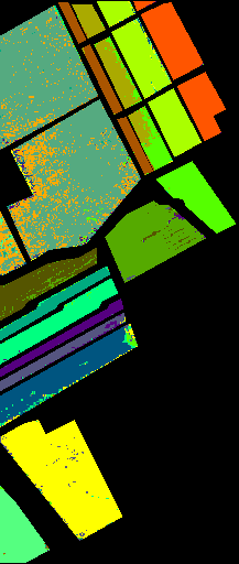
(d)

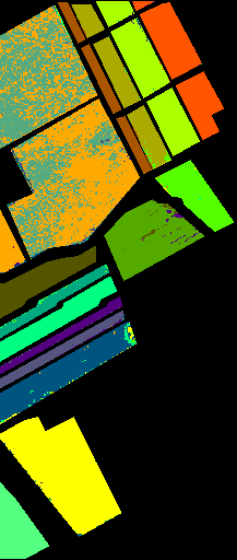
(e)

Figure 3: Label maps on Salinas using $13$ training samples per class. (a) ground truth (b) EMAP-PCA, (c) EMAP-PCA with 500 synthetic samples per class, (d) EMAP-NWFE, (e) EMAP-NWFE with 500 synthetic samples per class.

V Conclusion

A common issue in hyperspectral remote sensing image classification is the limited training data. This limitation severely challenges classifiers, particularly when using high dimensional feature vectors. In this work, we propose to compensate this limitation by adding synthetic samples drawn from a Gaussian mixture that is estimated on the feature space.

We show on the simulated data with non-Gaussian distributions that this idea indeed helps on severely limited training data, even if the true underlying distribution is only approximately matched (see supplemental material). In our results on real data, we show the performance gain for a standard dimensionality-reduction classification pipeline on the Pavia Centre, Pavia University and Salinas datasets. It turns out that synthetic samples consistently increase the OA, AA and kappa coefficient. After a performance jump when adding few features, the (improved) performance remains relatively stable when adding further synthetic features. Thus, the choice for the exact number of added features is not critical. Quantitatively, the exact performance improvement depends on the details of the processing chain and on the dataset. The mean improvement in our experiments is $4.5\%$, with variations between one percent and almost ten percent. These results are encouraging, as the approach itself is quite straightforward, and can be smoothly integrated into any classification pipeline.

GMM-Based Synthetic Samples for Classification of Hyperspectral Images With Limited Training Data
Supplementary Material

I Overview

This document contains the full experimental results to complement the results in the main text. We report results for all combinations of the two considered datasets (Pavia Centre and Salinas), two dimensionality-reduction methods (PCA and NWFE), two classifiers (random forests and SVM) with the purpose of either optimizing the classification parameters or adding synthetic samples. For training the classifiers, we used limited datasets of either 13, 20, 30, or 40 samples per class.

When considering an unoptimized random forest, default parameters from the literature are used, i.e., $H=100$ trees with a tree depth of the square root of the feature dimension, $D=\sqrt{d}$.

Furthermore, random forests are oftentimes used in the literature with a default set of variables rather than optimized parameters. We conducted each of the classification experiments using two versions of the classifiers: optimized and unoptimized. In our work, we denote a classifier as being “unoptimized” if its parameters are taken from reported values instead of being the results of a training protocol. In contrast, optimized classifiers result from a parameter search. In this document, we tabulate the full results to all of our experiments.

II Simulated Data

Since we are operating on limited training data, we consider a GMM as a reasonable trade-off between the model complexity and the expressiveness of the available samples. This is illustrated with a small simulation experiment. We generate three Gamma distributions with varying shape parameter $a$ and scale parameter $b$. These distributions are shown in Fig. 1(a). 1000, 2000 and 3000 samples are drawn from these distributions to simulate a gamma distributed dataset. From each dataset, 13 samples per class are randomly selected as the training set, and a GMM is fitted to each of these classes (with the same parametrization as for the real-world experiments stated further below). Then, we sample $0\leq n_{s}\leq 1000$ additional training samples from the estimated GMMs and add these samples to the original training set. A random forest classifier is trained on these $a+13$ samples. The parameters for random forest were chosen the same as what is popularly used in the hyperspectral remote sensing image analysis community, i.e. 100 trees ($H$) and square root of number of features as the maximum leaves depth ($D$), as in [19], [25], [27]. Fig. 1 shows the Cohen’s kappa of the classification result in dependency of the number of added samples $n_{s}$. It can be seen that the addition of very few synthetic samples already boosts classification performance. These performance gains remain roughly stable for up to $1000$ additional samples. The chosen GMM model is not able to accurately represent the Gamma distributions, which contributes to the fact that performance never reaches the optimum. However, it is sufficiently accurate to considerably improve the performance over the baseline with $500$ added samples.

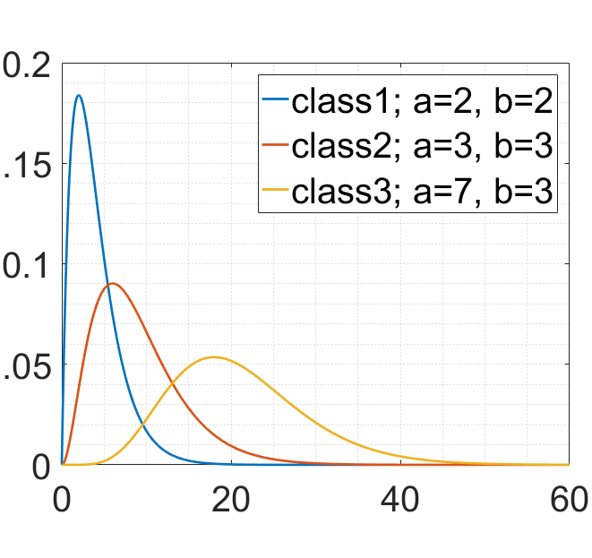
(a) Gamma distributions

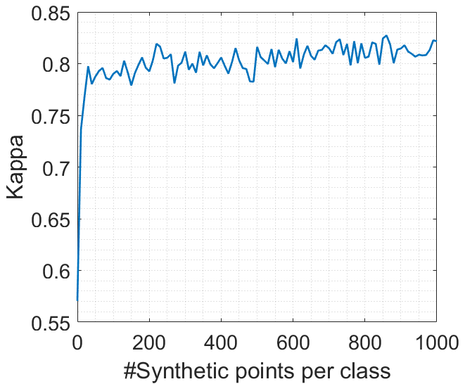
(b) Kappa

Figure 1: Simulation example on model accuracy versus classifier support: (a) three different gamma distributions serving as the simulated data’s class distributions, (b) classification performance (kappa value) vs. number of added synthetic samples drawn from the fitted GMM.

III Random Forest + Synthetic Samples

Tables 1 and 2 contain the classification results using the unoptimized random forest classifier. In Tab. 1, features are computed over Pavia Centre dataset and reduced via PCA and NWFE.

Table 1: Unoptimized random forest-based classification performance on Pavia Centre dataset with and without adding synthetic features.

Algorithm	$|S|$	AA% ($\pm$SD)	OA% ($\pm$SD)	Kappa ($\pm$SD)
Pavia Centre
13 pix/class
EMAP	-	77.87 ($\pm$2.97)	90.01 ($\pm$3.78)	0.8600 ($\pm$0.0495)
EMAP-PCA	-	73.51 ($\pm$3.00)	86.38 ($\pm$3.61)	0.8089 ($\pm$0.0493)
EMAP-PCA	500	84.59 ($\pm$1.58)	93.67 ($\pm$0.75)	0.9107 ($\pm$0.0104)
EMAP-NWFE	-	80.06 ($\pm$3.56)	91.37 ($\pm$2.67)	0.8787 ($\pm$0.0365)
EMAP-NWFE	500	89.57 ($\pm$1.15)	95.91 ($\pm$0.49)	0.9423 ($\pm$0.0069)
20 pix/class
EMAP	-	81.80 ($\pm$2.07)	92.73 ($\pm$1.23)	0.8974 ($\pm$0.0171)
EMAP-PCA	-	79.07 ($\pm$1.69)	90.89 ($\pm$1.22)	0.8717 ($\pm$0.0169)
EMAP-PCA	500	86.37 ($\pm$1.05)	94.16 ($\pm$0.47)	0.9178 ($\pm$0.0065)
EMAP-NWFE	-	83.32 ($\pm$2.24)	93.28 ($\pm$1.30)	0.9053 ($\pm$0.0181)
EMAP-NWFE	500	90.68 ($\pm$1.05)	96.17 ($\pm$0.50)	0.9460 ($\pm$0.0070)
30 pix/class
EMAP	-	85.57 ($\pm$1.29)	93.95 ($\pm$0.59)	0.9148 ($\pm$0.0082)
EMAP-PCA	-	82.19 ($\pm$1.29)	92.97 ($\pm$0.75)	0.9008 ($\pm$0.0105)
EMAP-PCA	500	87.91 ($\pm$1.09)	94.75 ($\pm$0.48)	0.9260 ($\pm$0.0067)
EMAP-NWFE	-	86.69 ($\pm$1.12)	94.89 ($\pm$0.74)	0.9279 ($\pm$0.0103)
EMAP-NWFE	500	91.70 ($\pm$0.90)	96.53 ($\pm$0.56)	0.9510 ($\pm$0.0078)
40 pix/class
EMAP	-	86.80 ($\pm$1.47)	94.30 ($\pm$0.61)	0.9197 ($\pm$0.0086)
EMAP-PCA	-	83.98 ($\pm$1.18)	93.49 ($\pm$0.69)	0.9082 ($\pm$0.0096)
EMAP-PCA	500	88.74 ($\pm$0.96)	95.09 ($\pm$0.54)	0.9307 ($\pm$0.0076)
EMAP-NWFE	-	87.41 ($\pm$1.41)	95.18 ($\pm$0.61)	0.9318 ($\pm$0.0085)
EMAP-NWFE	500	92.39 ($\pm$0.75)	96.66 ($\pm$0.46)	0.9528 ($\pm$0.0063)

Analogously, Tab. 2 presents unoptimized random forest performance for features from EMAP, EMAP-PCA and EMAP-NWFE, with and without synthetic samples, computed over Salinas dataset. $|S|$ represents the number of added synthetic samples.

Table 2: Unoptimized random forest performance on Salinas dataset with and without adding synthetic features.

Algorithm	$|S|$	AA% ($\pm$SD)	OA% ($\pm$SD)	Kappa ($\pm$SD)
Salinas
13 pix/class
EMAP	-	83.84 ($\pm$2.06)	76.30 ($\pm$2.74)	0.7380 ($\pm$0.0292)
EMAP-PCA	-	82.50 ($\pm$2.06)	74.96 ($\pm$3.63)	0.7230 ($\pm$0.0378)
EMAP-PCA	500	90.96 ($\pm$0.88)	83.89 ($\pm$1.72)	0.8215 ($\pm$0.0188)
EMAP-NWFE	-	88.68 ($\pm$1.20)	80.42 ($\pm$2.34)	0.7838 ($\pm$0.0247)
EMAP-NWFE	500	93.17 ($\pm$0.68)	87.09 ($\pm$1.26)	0.8566 ($\pm$0.0138)
20 pix/class
EMAP	-	86.81 ($\pm$1.63)	79.74 ($\pm$2.56)	0.7756 ($\pm$0.0269)
EMAP-PCA	-	86.59 ($\pm$1.06)	78.70 ($\pm$2.33)	0.7643 ($\pm$0.0249)
EMAP-PCA	500	91.76 ($\pm$0.97)	85.38 ($\pm$1.40)	0.8376 ($\pm$0.0154)
EMAP-NWFE	-	90.56 ($\pm$1.26)	82.26 ($\pm$2.62)	0.8038 ($\pm$0.0280)
EMAP-NWFE	500	94.00 ($\pm$0.39)	88.28 ($\pm$1.01)	0.8697 ($\pm$0.0111)
30 pix/class
EMAP	-	89.01 ($\pm$1.10)	81.80 ($\pm$2.30)	0.7985 ($\pm$0.0248)
EMAP-PCA	-	88.85 ($\pm$0.91)	80.96 ($\pm$2.15)	0.7895 ($\pm$0.0229)
EMAP-PCA	500	92.63 ($\pm$0.47)	86.27 ($\pm$0.94)	0.8476 ($\pm$0.0103)
EMAP-NWFE	-	92.25 ($\pm$0.82)	84.76 ($\pm$2.38)	0.8314 ($\pm$0.0256)
EMAP-NWFE	500	94.35 ($\pm$0.43)	88.74 ($\pm$1.24)	0.8748 ($\pm$0.0138)
40 pix/class
EMAP	-	90.75 ($\pm$0.86)	84.52 ($\pm$1.76)	0.8285 ($\pm$0.0192)
EMAP-PCA	-	89.80 ($\pm$1.21)	81.73 ($\pm$2.51)	0.7981 ($\pm$0.0273)
EMAP-PCA	500	93.08 ($\pm$0.40)	86.59 ($\pm$0.85)	0.8512 ($\pm$0.0093)
EMAP-NWFE	-	93.29 ($\pm$0.41)	86.09 ($\pm$1.86)	0.8462 ($\pm$0.0200)
EMAP-NWFE	500	94.52 ($\pm$0.30)	89.18 ($\pm$0.81)	0.8798 ($\pm$0.0089)

As it was mentioned in the main paper, to further evaluate our idea and compare with other works, we conducted our experiments on the commonly used Pavia University dataset. Tab. 3 presents unoptimized random forest performance for features from EMAP, EMAP-PCA and EMAP-NWFE, with and without synthetic samples, computed over Pavia University dataset. $|S|$ represents the number of added synthetic samples.

Table 3: Unoptimized random forest performance on Pavia University dataset with and without adding synthetic features.

Algorithm	$|S|$	AA% ($\pm$SD)	OA% ($\pm$SD)	Kappa ($\pm$SD)
Pavia University
13 pix/class
EMAP	-	70.50 ($\pm$2.88)	54.81 ($\pm$7.72)	0.4625 ($\pm$0.0734)
EMAP-PCA	-	73.77 ($\pm$3.56)	65.59 ($\pm$8.52)	0.5726 ($\pm$0.0879)
EMAP-PCA	500	84.78 ($\pm$1.49)	79.52 ($\pm$2.98)	0.7376 ($\pm$0.0344)
EMAP-NWFE	-	68.33 ($\pm$2.97)	62.90 ($\pm$6.89)	0.5369 ($\pm$0.0671)
EMAP-NWFE	500	82.87 ($\pm$1.09)	76.13 ($\pm$3.12)	0.6984 ($\pm$0.0340)
20 pix/class
EMAP	-	75.93 ($\pm$2.00)	65.12 ($\pm$4.74)	0.5691 ($\pm$0.0467)
EMAP-PCA	-	78.73 ($\pm$2.28)	74.87 ($\pm$5.94)	0.6768 ($\pm$0.0621)
EMAP-PCA	500	86.75 ($\pm$1.16)	82.24 ($\pm$3.13)	0.7717 ($\pm$0.0364)
EMAP-NWFE	-	76.87 ($\pm$2.13)	72.13 ($\pm$7.01)	0.6466 ($\pm$0.0715)
EMAP-NWFE	500	83.96 ($\pm$1.20)	77.84 ($\pm$2.57)	0.7183 ($\pm$0.0291)
30 pix/class
EMAP	-	79.63 ($\pm$1.56)	70.94 ($\pm$3.55)	0.6353 ($\pm$0.0375)
EMAP-PCA	-	83.04 ($\pm$1.46)	77.76 ($\pm$4.75)	0.7156 ($\pm$0.0495)
EMAP-PCA	500	87.55 ($\pm$0.87)	83.05 ($\pm$2.29)	0.7818 ($\pm$0.0266)
EMAP-NWFE	-	80.08 ($\pm$1.68)	75.16 ($\pm$4.95)	0.6819 ($\pm$0.0528)
EMAP-NWFE	500	85.61 ($\pm$0.83)	80.44 ($\pm$2.56)	0.7502 ($\pm$0.0296)
40 pix/class
EMAP	-	81.72 ($\pm$1.52)	71.16 ($\pm$3.61)	0.6422 ($\pm$0.0379)
EMAP-PCA	-	84.85 ($\pm$1.10)	79.71 ($\pm$3.42)	0.7392 ($\pm$0.0381)
EMAP-PCA	500	88.36 ($\pm$1.03)	83.72 ($\pm$2.27)	0.7907 ($\pm$0.0266)
EMAP-NWFE	-	81.71 ($\pm$1.35)	76.47 ($\pm$4.36)	0.6996 ($\pm$0.0473)
EMAP-NWFE	500	86.07 ($\pm$0.93)	80.86 ($\pm$2.85)	0.7557 ($\pm$0.0329)

IV SVM + Synthetic Samples

Tab. 4 shows the classification results of EMAP, EMAP-PCA, EMAP-NWFE and variants thereof with added synthetic samples, computed over Pavia Centre dataset, using an unoptimized SVM classifier. Similarly, Tab. 5 exhibits the unoptimized SVM results of the same features, but computed over Salinas datasets.

Table 4: Unoptimized SVM performance on Pavia Centre with and without adding synthetic features. Parameters of SVM are arbitrarily chosen to be $C=1$ and $\gamma=5$ for both EMAP-PCA and EMAP-NWFE datasets.

Algorithm	$|S|$	AA% ($\pm$SD)	OA% ($\pm$SD)	Kappa ($\pm$SD)
Pavia Centre
13 pix/class
EMAP	-	89.77 ($\pm$1.75)	95.37 ($\pm$0.89)	0.9348 ($\pm$0.0124)
EMAP-PCA	-	75.11 ($\pm$2.21)	90.41 ($\pm$1.28)	0.8627 ($\pm$0.0188)
EMAP-PCA	500	87.01 ($\pm$1.08)	94.68 ($\pm$0.48)	0.9249 ($\pm$0.0067)
EMAP-NWFE	-	77.27 ($\pm$1.69)	91.96 ($\pm$1.09)	0.8851 ($\pm$0.0157)
EMAP-NWFE	500	90.01 ($\pm$0.87)	95.32 ($\pm$0.35)	0.9341 ($\pm$0.0049)
20 pix/class
EMAP	-	90.92 ($\pm$1.23)	96.27 ($\pm$0.52)	0.9473 ($\pm$0.0073)
EMAP-PCA	-	78.45 ($\pm$1.42)	91.87 ($\pm$0.72)	0.8844 ($\pm$0.0105)
EMAP-PCA	500	87.51 ($\pm$1.42)	94.96 ($\pm$0.50)	0.9289 ($\pm$0.0071)
EMAP-NWFE	-	78.91 ($\pm$1.49)	92.37 ($\pm$0.71)	0.8915 ($\pm$0.0102)
EMAP-NWFE	500	91.14 ($\pm$0.64)	95.74 ($\pm$0.29)	0.9400 ($\pm$0.0040)
30 pix/class
EMAP	-	93.31 ($\pm$0.59)	97.01 ($\pm$0.37)	0.9578 ($\pm$0.0052)
EMAP-PCA	-	80.79 ($\pm$1.71)	92.80 ($\pm$0.83)	0.8977 ($\pm$0.0119)
EMAP-PCA	500	89.05 ($\pm$0.39)	95.63 ($\pm$0.36)	0.9382 ($\pm$0.0049)
EMAP-NWFE	-	82.63 ($\pm$1.23)	94.40 ($\pm$0.52)	0.9206 ($\pm$0.0073)
EMAP-NWFE	500	91.15 ($\pm$0.76)	96.41 ($\pm$0.09)	0.9493 ($\pm$0.0013)
40 pix/class
EMAP	-	93.74 ($\pm$0.61)	97.05 ($\pm$0.43)	0.9584 ($\pm$0.0060)
EMAP-PCA	-	83.52 ($\pm$1.38)	93.95 ($\pm$0.55)	0.9142 ($\pm$0.0078)
EMAP-PCA	500	88.83 ($\pm$0.83)	95.39 ($\pm$0.25)	0.9348 ($\pm$0.0035)
EMAP-NWFE	-	83.52 ($\pm$0.98)	93.99 ($\pm$0.42)	0.9150 ($\pm$0.0060)
EMAP-NWFE	500	92.13 ($\pm$0.31)	96.42 ($\pm$0.31)	0.9495 ($\pm$0.0043)

Table 5: Unoptimized SVM performance on Salinas with and without adding synthetic features. Parameters of SVM are arbitrarily chosen to be $C=1$ and $\gamma=1$ for EMAP-PCA dataset and $C=1$ and $\gamma=5$ for EMAP-NWFE dataset.

Algorithm	$|S|$	AA% ($\pm$SD)	OA% ($\pm$SD)	Kappa ($\pm$SD)
Salinas
13 pix/class
EMAP	-	89.47 ($\pm$1.13)	80.82 ($\pm$1.33)	0.7886 ($\pm$0.0146)
EMAP-PCA	-	88.45 ($\pm$0.50)	79.60 ($\pm$1.95)	0.7749 ($\pm$0.0204)
EMAP-PCA	500	92.69 ($\pm$0.74)	85.74 ($\pm$1.94)	0.8420 ($\pm$0.0212)
EMAP-NWFE	-	84.23 ($\pm$1.32)	75.21 ($\pm$3.23)	0.7266 ($\pm$0.0332)
EMAP-NWFE	500	93.21 ($\pm$0.69)	86.34 ($\pm$1.83)	0.8485 ($\pm$0.0202)
20 pix/class
EMAP	-	91.17 ($\pm$0.66)	83.47 ($\pm$1.12)	0.8174 ($\pm$0.0123)
EMAP-PCA	-	89.87 ($\pm$0.83)	83.00 ($\pm$1.74)	0.8119 ($\pm$0.0187)
EMAP-PCA	500	92.75 ($\pm$0.94)	85.90 ($\pm$1.63)	0.8438 ($\pm$0.0179)
EMAP-NWFE	-	84.15 ($\pm$0.64)	75.91 ($\pm$2.12)	0.7346 ($\pm$0.0223)
EMAP-NWFE	500	93.96 ($\pm$0.29)	87.69 ($\pm$1.28)	0.8635 ($\pm$0.0140)
30 pix/class
EMAP	-	92.31 ($\pm$0.54)	84.80 ($\pm$0.92)	0.8320 ($\pm$0.0100)
EMAP-PCA	-	90.64 ($\pm$0.91)	82.06 ($\pm$2.23)	0.8021 ($\pm$0.0239)
EMAP-PCA	500	93.76 ($\pm$0.44)	87.63 ($\pm$0.70)	0.8628 ($\pm$0.0078)
EMAP-NWFE	-	84.80 ($\pm$0.52)	75.20 ($\pm$2.31)	0.7270 ($\pm$0.0237)
EMAP-NWFE	500	93.94 ($\pm$0.32)	88.57 ($\pm$0.35)	0.8730 ($\pm$0.0039)
40 pix/class
EMAP	-	92.88 ($\pm$0.45)	85.79 ($\pm$1.23)	0.8429 ($\pm$0.0134)
EMAP-PCA	-	91.40 ($\pm$0.93)	83.60 ($\pm$2.47)	0.8190 ($\pm$0.0266)
EMAP-PCA	500	93.84 ($\pm$0.50)	87.67 ($\pm$1.25)	0.8632 ($\pm$0.0137)
EMAP-NWFE	-	87.08 ($\pm$2.29)	78.00 ($\pm$4.44)	0.7580 ($\pm$0.0476)
EMAP-NWFE	500	94.13 ($\pm$0.33)	88.70 ($\pm$0.83)	0.8745 ($\pm$0.0092)

V Classifier Parameter Selection

When using, e.g., the support vector machine classifier (SVM), it is widely known that parameter selection is a critical preparatory step towards obtaining competitive results. This is the reason why, for example, SVM parameter selection is hardwired into the popular SVM implementation libSVM. However, other classification frameworks do not necessarily include a parameter selection submodule. One notable example is classification with a random forest. Several works [28, 27, 29, 30, 31, 16] rely on the default settings of $100$ trees with a tree depth equal to the square root of the feature dimensionality, $\sqrt{d}$, as originally proposed by Breiman [24]. However, these parameters have been proposed based on training on a relatively large dataset. In the case of classification on severely limited training data, such default parameters yield suboptimal classification performance.

To illustrate how far off the default parameters can be from the optimum solution, we show two example results in Fig. 2. A similar study for large training sets has been done by Rodriguez-Galiano et al.[32]. We used limited training sets of size $13$ and $40$, respectively. The features are extracted from Pavia Centre dataset using PCA-reduced EMAP features, and from Salinas dataset using NWFE-reduced EMAP features, respectively. We color-code the kappa classification performance for different random forest configurations, i.e., different numbers of trees and tree depths. In both examples, considerably smaller number of trees perform significantly better.

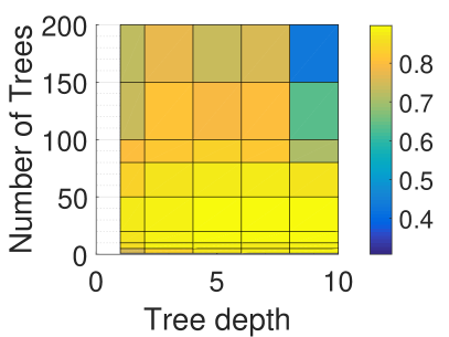
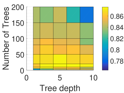
Figure 2: Random forest kappa performance using different number of trees $H$ and tree depths $D$. Left: Pavia-EMAP-PCA with training set size of $13$ pixels per class. Right: Salinas-EMAP-NWFE with training set size of $40$ pixels per class.

V-A Optimized Parameters for Random Forest

Classification performance of optimized random forest classifier on EMAP and EMAP-reduced features computed over Pavia Centre and Salinas dataset are shown in Tab. 6 and Tab. 7, respectively. The optimized parameters of random forest, $H$ and $D$, are also listed in the tables.

Table 6: Optimized random forest-based classification performance on Pavia Centre dataset without adding synthetic features. $H$ and $D$ represent the tuned parameters of random forest.

Algorithm	$H$	$D$	AA% ($\pm$SD)	OA% ($\pm$SD)	Kappa ($\pm$SD)
13 pix/class
EMAP	5	4	86.55 ($\pm$1.73)	93.99 ($\pm$1.11)	0.9154 ($\pm$0.0151)
EMAP-PCA	10	8	84.05 ($\pm$1.44)	92.67 ($\pm$0.82)	0.8970 ($\pm$0.0113)
EMAP-NWFE	10	4	87.38 ($\pm$1.04)	94.86 ($\pm$0.47)	0.9276 ($\pm$0.0066)
20 pix/class
EMAP	10	10	89.59 ($\pm$1.24)	94.94 ($\pm$0.76)	0.9289 ($\pm$0.0106)
EMAP-PCA	20	10	86.21 ($\pm$1.24)	93.80 ($\pm$0.53)	0.9128 ($\pm$0.0074)
EMAP-NWFE	20	2	88.01 ($\pm$0.97)	95.21 ($\pm$0.56)	0.9325 ($\pm$0.0079)
30 pix/class
EMAP	10	6	90.84 ($\pm$1.08)	95.60 ($\pm$0.62)	0.9381 ($\pm$0.0087)
EMAP-PCA	10	8	87.47 ($\pm$0.79)	94.22 ($\pm$0.38)	0.9187 ($\pm$0.0053)
EMAP-NWFE	20	4	90.16 ($\pm$0.92)	95.86 ($\pm$0.51)	0.9416 ($\pm$0.0072)
40 pix/class
EMAP	10	10	92.67 ($\pm$0.74)	96.03 ($\pm$0.73)	0.9441 ($\pm$0.0101)
EMAP-PCA	10	6	88.97 ($\pm$0.97)	94.84 ($\pm$0.67)	0.9274 ($\pm$0.0093)
EMAP-NWFE	20	2	90.90 ($\pm$0.96)	96.17 ($\pm$0.48)	0.9459 ($\pm$0.0068)

Table 7: Optimized random forest-based classification performance on Salinas dataset without adding synthetic features. $H$ and $D$ represent the tuned parameters of random forest.

Algorithm	$H$	$D$	AA% ($\pm$SD)	OA% ($\pm$SD)	Kappa ($\pm$SD)
13 pix/class
EMAP	5	10	91.54 ($\pm$1.06)	86.45 ($\pm$2.25)	0.8496 ($\pm$0.0250)
EMAP-PCA	10	6	89.29 ($\pm$1.10)	82.66 ($\pm$1.39)	0.8077 ($\pm$0.0153)
EMAP-NWFE	10	4	91.85 ($\pm$0.89)	85.21 ($\pm$1.18)	0.8357 ($\pm$0.0132)
20 pix/class
EMAP	5	10	93.10 ($\pm$0.93)	88.13 ($\pm$1.86)	0.8683 ($\pm$0.0206)
EMAP-PCA	10	10	90.68 ($\pm$0.73)	84.14 ($\pm$1.21)	0.8241 ($\pm$0.0133)
EMAP-NWFE	20	6	92.75 ($\pm$0.54)	86.58 ($\pm$0.94)	0.8511 ($\pm$0.0103)
30 pix/class
EMAP	5	10	94.33 ($\pm$0.93)	90.32 ($\pm$1.40)	0.8926 ($\pm$0.0155)
EMAP-PCA	10	10	91.67 ($\pm$0.73)	85.58 ($\pm$0.68)	0.8399 ($\pm$0.0076)
EMAP-NWFE	10	4	93.83 ($\pm$0.43)	88.11 ($\pm$0.92)	0.8679 ($\pm$0.0101)
40 pix/class
EMAP	5	10	95.13 ($\pm$0.71)	91.55 ($\pm$1.08)	0.9062 ($\pm$0.0119)
EMAP-PCA	10	4	92.43 ($\pm$0.33)	86.38 ($\pm$0.52)	0.8489 ($\pm$0.0058)
EMAP-NWFE	10	6	94.20 ($\pm$0.30)	88.83 ($\pm$0.88)	0.8760 ($\pm$0.0097)

V-B Optimized Parameters for SVM

Analogously to Sec. V-A, Tab. 8 and Tab. 9 show the classification results using an optimized SVM on Pavia Centre and Salinas datasets, respectively. As SVM classifier is by design a two class classifier, we use a one-versus-all approach to multi-class classification. For classifier tuning, the parameters for each classifier result from a grid-search. Thus, each classifier obtains a unique set of parameters $C$ and $\gamma$. Therefore, there is not a single best set of parameters for the overall classifier, which is why these parameters are not reported here.

Table 8: Tuned SVM-based classification performance of EMAP, EMAP-PCA and EMAP-NWFE computed over Pavia Centre dataset without adding synthetic features.

Algorithm	AA% ($\pm$SD)	OA% ($\pm$SD)	Kappa ($\pm$SD)
13 pix/class
EMAP	87.20 ($\pm$1.53)	94.24 ($\pm$1.07)	0.9189 ($\pm$0.0148)
EMAP-PCA	86.21 ($\pm$2.83)	93.85 ($\pm$1.10)	0.9134 ($\pm$0.0154)
EMAP-NWFE	88.42 ($\pm$1.48)	94.86 ($\pm$0.68)	0.9276 ($\pm$0.0095)
20 pix/class
EMAP	90.77 ($\pm$1.42)	95.64 ($\pm$0.67)	0.9385 ($\pm$0.0094)
EMAP-PCA	88.41 ($\pm$1.35)	94.82 ($\pm$0.64)	0.9269 ($\pm$0.0089)
EMAP-NWFE	90.72 ($\pm$1.51)	95.60 ($\pm$0.70)	0.9380 ($\pm$0.0099)
30 pix/class
EMAP	92.57 ($\pm$0.85)	96.16 ($\pm$0.39)	0.9459 ($\pm$0.0055)
EMAP-PCA	91.46 ($\pm$0.96)	95.90 ($\pm$0.57)	0.9422 ($\pm$0.0080)
EMAP-NWFE	92.27 ($\pm$0.89)	96.28 ($\pm$0.47)	0.9475 ($\pm$0.0065)
40 pix/class
EMAP	93.61 ($\pm$0.84)	96.97 ($\pm$0.52)	0.9573 ($\pm$0.0073)
EMAP-PCA	92.55 ($\pm$1.18)	96.45 ($\pm$0.46)	0.9500 ($\pm$0.0064)
EMAP-NWFE	93.46 ($\pm$0.80)	96.82 ($\pm$0.36)	0.9551 ($\pm$0.0051)

Table 9: Tuned SVM-based classification performance of EMAP, EMAP-PCA and EMAP-NWFE computed over Salinas dataset without adding synthetic features.

Algorithm	AA% ($\pm$SD)	OA% ($\pm$SD)	Kappa ($\pm$SD)
13 pix/class
EMAP	93.55 ($\pm$0.60)	87.41 ($\pm$1.35)	0.8604 ($\pm$0.0149)
EMAP-PCA	91.73 ($\pm$1.01)	84.57 ($\pm$1.96)	0.8292 ($\pm$0.0213)
EMAP-NWFE	93.78 ($\pm$0.90)	87.94 ($\pm$1.88)	0.8660 ($\pm$0.0208)
20 pix/class
EMAP	94.69 ($\pm$0.64)	89.92 ($\pm$1.44)	0.8880 ($\pm$0.0160)
EMAP-PCA	93.02 ($\pm$0.47)	86.45 ($\pm$1.15)	0.8497 ($\pm$0.0126)
EMAP-NWFE	94.86 ($\pm$0.47)	89.96 ($\pm$1.47)	0.8885 ($\pm$0.0163)
30 pix/class
EMAP	95.28 ($\pm$0.45)	91.22 ($\pm$1.40)	0.9025 ($\pm$0.0155)
EMAP-PCA	93.81 ($\pm$0.48)	87.57 ($\pm$1.18)	0.8621 ($\pm$0.0131)
EMAP-NWFE	95.54 ($\pm$0.49)	91.91 ($\pm$1.25)	0.9101 ($\pm$0.0138)
40 pix/class
EMAP	95.91 ($\pm$0.48)	92.20 ($\pm$1.15)	0.9134 ($\pm$0.0127)
EMAP-PCA	94.08 ($\pm$0.60)	87.96 ($\pm$1.58)	0.8664 ($\pm$0.0173)
EMAP-NWFE	95.79 ($\pm$0.43)	92.07 ($\pm$1.07)	0.9118 ($\pm$0.0120)

V-C Performances for Various Random Forest Parameters

Fig. 2 shows that the classical parameters which are used in the literature for random forest classifier, i.e., number of trees $H=100$, and depth, $D=\sqrt{d}$, are not the optimal parameter values, particularly for severely limited training data sizes. This conclusion was drawn based on the experiments conducted over EMAP-PCA and EMAP-NWFE computed over Pavia Centre and Salinas datasets. Fig. 2 illustrates instances of the numerical analysis which are presented in Tables 10, 11, 12, 13.

Table 10: Kappa-based parameter search results for random forest classifier over EMAP-PCA computed on Pavia Centre dataset.

	1	2	4	6	8	10
13 pix/class
1	0.7525	0.8343	0.8689	0.8766	0.8861	0.8851
5	0.8594	0.8795	0.8832	0.8784	0.8815	0.8916
10	0.8661	0.8853	0.8945	0.8926	0.8970	0.8967
20	0.8739	0.8820	0.8927	0.8942	0.8958	0.8922
50	0.8351	0.8680	0.8723	0.8755	0.8605	0.8546
80	0.8036	0.8228	0.8353	0.8150	0.7119	0.6854
100	0.7371	0.8121	0.7921	0.7958	0.6362	0.6398
150	0.7298	0.7739	0.7318	0.7503	0.4314	0.4827
200	0.7298	0.7105	0.6883	0.7079	0.3070	0.3065
20 pix/class
1	0.7484	0.8587	0.8818	0.8891	0.9002	0.9005
5	0.8683	0.8951	0.9043	0.8942	0.8971	0.8983
10	0.8912	0.9047	0.9068	0.9090	0.9040	0.9082
20	0.8899	0.8999	0.9083	0.9037	0.9026	0.9128
50	0.8854	0.8884	0.9029	0.8974	0.8941	0.8983
80	0.8543	0.8707	0.8832	0.8803	0.8676	0.8649
100	0.8475	0.8742	0.8745	0.8574	0.8404	0.8359
150	0.7959	0.8355	0.8348	0.8515	0.7029	0.6732
200	0.8049	0.8195	0.8236	0.7921	0.5885	0.5609
30 pix/class
1	0.7813	0.8547	0.8957	0.8946	0.9126	0.9142
5	0.8941	0.9070	0.9094	0.9095	0.9093	0.9095
10	0.8988	0.9184	0.9139	0.9182	0.9187	0.9174
20	0.9083	0.9130	0.9123	0.9153	0.9131	0.9177
50	0.8994	0.9067	0.9104	0.9132	0.9074	0.9061
80	0.8945	0.9043	0.9047	0.9083	0.9010	0.9075
100	0.8818	0.8941	0.8978	0.8989	0.8968	0.8959
150	0.8610	0.8884	0.8911	0.8856	0.8438	0.8619
200	0.8437	0.8572	0.8606	0.8697	0.7828	0.7769
40 pix/class
1	0.8319	0.8676	0.9027	0.9111	0.9186	0.9174
5	0.9004	0.9188	0.9183	0.9176	0.9178	0.9153
10	0.9101	0.9242	0.9262	0.9274	0.9208	0.9247
20	0.9127	0.9208	0.9215	0.9165	0.9216	0.9249
50	0.9066	0.9164	0.9157	0.9152	0.9139	0.9114
80	0.8974	0.9094	0.9132	0.9104	0.9084	0.9084
100	0.8898	0.9068	0.9099	0.9140	0.9085	0.9026
150	0.8904	0.9009	0.9060	0.9028	0.8908	0.8879
200	0.8813	0.8842	0.9018	0.8958	0.8664	0.8563

Table 11: Kappa-based parameter search results for random forest classifier over EMAP-NWFE computed on Pavia Centre dataset.

	1	2	4	6	8	10
13 pix/class
1	0.7776	0.8501	0.8576	0.8648	0.8700	0.8607
5	0.8749	0.8985	0.8779	0.8687	0.8701	0.8811
10	0.8963	0.9201	0.9276	0.9026	0.9147	0.9110
20	0.9042	0.9213	0.9276	0.9126	0.9183	0.9097
50	0.9103	0.9057	0.9116	0.8664	0.8702	0.8840
80	0.8894	0.8848	0.8962	0.7640	0.7882	0.7883
100	0.8620	0.8924	0.8896	0.7338	0.7662	0.7743
150	0.8561	0.8819	0.8672	0.6658	0.6528	0.6770
200	0.8145	0.8298	0.8356	0.5222	0.5605	0.5210
20 pix/class
1	0.8265	0.8721	0.8859	0.8800	0.8949	0.8951
5	0.9025	0.9143	0.8978	0.8912	0.9033	0.8964
10	0.9175	0.9312	0.9320	0.9199	0.9234	0.9262
20	0.9139	0.9325	0.9322	0.9254	0.9277	0.9221
50	0.9099	0.9177	0.9259	0.9135	0.9224	0.9129
80	0.9086	0.9162	0.9228	0.8762	0.8785	0.8826
100	0.9028	0.9119	0.9174	0.8474	0.8495	0.8471
150	0.8999	0.9025	0.9029	0.7952	0.7757	0.7639
200	0.8946	0.8884	0.8914	0.7389	0.7318	0.7202
30 pix/class
1	0.8463	0.8877	0.9088	0.9133	0.9076	0.9150
5	0.9118	0.9290	0.9168	0.9030	0.9107	0.9135
10	0.9299	0.9379	0.9388	0.9322	0.9334	0.9312
20	0.9330	0.9377	0.9416	0.9337	0.9345	0.9311
50	0.9276	0.9375	0.9380	0.9288	0.9301	0.9318
80	0.9205	0.9314	0.9317	0.9195	0.9190	0.9195
100	0.9205	0.9300	0.9320	0.9124	0.9069	0.9094
150	0.9203	0.9186	0.9197	0.8725	0.8689	0.8791
200	0.9154	0.9160	0.9097	0.8019	0.7994	0.8334
40 pix/class
1	0.8522	0.8997	0.9095	0.9153	0.9147	0.9181
5	0.9285	0.9359	0.9288	0.9141	0.9183	0.9243
10	0.9353	0.9458	0.9375	0.9361	0.9404	0.9356
20	0.9383	0.9459	0.9433	0.9404	0.9393	0.9404
50	0.9371	0.9413	0.9438	0.9351	0.9364	0.9358
80	0.9337	0.9356	0.9351	0.9272	0.9316	0.9276
100	0.9288	0.9379	0.9373	0.9267	0.9296	0.9257
150	0.9276	0.9319	0.9329	0.9012	0.9101	0.9028
200	0.9183	0.9268	0.9251	0.8697	0.8786	0.8728

Table 12: Kappa-based parameter search results for random forest classifier over EMAP-PCA computed on Salinas dataset.

	1	2	4	6	8	10
13 pix/class
1	0.7350	0.7730	0.7809	0.7840	0.7891	0.7811
5	0.7963	0.7988	0.7873	0.7851	0.7888	0.7793
10	0.7919	0.7963	0.8054	0.8077	0.8066	0.7956
20	0.7841	0.7834	0.7883	0.7910	0.7912	0.7935
50	0.7534	0.7609	0.7596	0.7618	0.7587	0.7512
80	0.7455	0.7357	0.7024	0.7012	0.7187	0.6991
100	0.7259	0.7134	0.6567	0.6726	0.6674	0.6526
150	0.6825	0.7026	0.6043	0.5972	0.6153	0.5930
200	0.6903	0.6741	0.5520	0.5545	0.5609	0.5497
20 pix/class
1	0.7545	0.7876	0.8051	0.8003	0.7994	0.7987
5	0.8010	0.8135	0.7930	0.7961	0.7993	0.8027
10	0.8104	0.8184	0.8235	0.8099	0.8164	0.8241
20	0.8013	0.8172	0.8117	0.8030	0.8118	0.8050
50	0.7849	0.7817	0.7898	0.7951	0.7826	0.7856
80	0.7699	0.7792	0.7571	0.7621	0.7642	0.7565
100	0.7508	0.7685	0.7437	0.7472	0.7544	0.7411
150	0.7352	0.7453	0.6962	0.6921	0.6850	0.6897
200	0.7251	0.7293	0.6581	0.6392	0.6389	0.6290
30 pix/class
1	0.7764	0.7998	0.8174	0.8184	0.8197	0.8155
5	0.8287	0.8326	0.8179	0.8153	0.8140	0.8137
10	0.8317	0.8380	0.8380	0.8340	0.8376	0.8399
20	0.8153	0.8287	0.8294	0.8269	0.8323	0.8320
50	0.8040	0.8055	0.8088	0.8058	0.8123	0.8083
80	0.7924	0.7881	0.7907	0.7934	0.7900	0.7877
100	0.7927	0.7861	0.7783	0.7799	0.7791	0.7936
150	0.7621	0.7704	0.7588	0.7482	0.7570	0.7596
200	0.7557	0.7523	0.7220	0.7226	0.7123	0.7248
40 pix/class
1	0.7904	0.8157	0.8272	0.8216	0.8327	0.8250
5	0.8350	0.8402	0.8210	0.8282	0.8271	0.8252
10	0.8396	0.8489	0.8489	0.8452	0.8477	0.8437
20	0.8334	0.8434	0.8425	0.8421	0.8342	0.8422
50	0.8114	0.8253	0.8103	0.8207	0.8283	0.8262
80	0.8081	0.8146	0.8059	0.8083	0.8129	0.8114
100	0.8083	0.8008	0.7962	0.8017	0.7960	0.8022
150	0.7804	0.7780	0.7876	0.7830	0.7769	0.7899
200	0.7732	0.7805	0.7639	0.7628	0.7657	0.7703

Table 13: Kappa-based parameter search results for random forest classifier over EMAP-NWFE computed on Salinas dataset.

	1	2	4	6	8	10
13 pix/class
1	0.7471	0.7813	0.8001	0.7941	0.7941	0.7956
5	0.8083	0.8223	0.8221	0.8110	0.7917	0.7933
10	0.8232	0.8312	0.8357	0.8296	0.8258	0.8247
20	0.8171	0.8171	0.8315	0.8208	0.8220	0.8106
50	0.8031	0.7893	0.7967	0.7979	0.7547	0.7587
80	0.7854	0.7755	0.7969	0.7834	0.6499	0.6589
100	0.7820	0.7817	0.7820	0.7714	0.5493	0.5664
150	0.7698	0.7677	0.7756	0.7628	0.4025	0.4156
200	0.7518	0.7458	0.7407	0.7596	0.3003	0.3041
20 pix/class
1	0.7434	0.8012	0.8135	0.8203	0.8267	0.8220
5	0.8337	0.8447	0.8401	0.8294	0.8243	0.8242
10	0.8349	0.8473	0.8493	0.8497	0.8456	0.8490
20	0.8370	0.8443	0.8457	0.8511	0.8382	0.8345
50	0.8239	0.8233	0.8238	0.8313	0.8153	0.8165
80	0.8035	0.8133	0.8060	0.8248	0.7714	0.7744
100	0.7989	0.8067	0.7946	0.7928	0.7250	0.7318
150	0.7930	0.7933	0.7995	0.8001	0.6332	0.6135
200	0.7885	0.7832	0.7755	0.7842	0.4812	0.4911
30 pix/class
1	0.7860	0.8146	0.8347	0.8457	0.8380	0.8327
5	0.8542	0.8523	0.8571	0.8422	0.8410	0.8377
10	0.8550	0.8656	0.8679	0.8652	0.8642	0.8675
20	0.8555	0.8565	0.8590	0.8575	0.8586	0.8560
50	0.8357	0.8439	0.8410	0.8487	0.8444	0.8422
80	0.8371	0.8346	0.8392	0.8323	0.8197	0.8283
100	0.8345	0.8340	0.8240	0.8288	0.7964	0.8053
150	0.8134	0.8237	0.8158	0.8215	0.7589	0.7316
200	0.8222	0.8289	0.8058	0.8128	0.6626	0.6791
40 pix/class
1	0.8019	0.8289	0.8436	0.8488	0.8471	0.8431
5	0.8610	0.8712	0.8612	0.8589	0.8420	0.8483
10	0.8602	0.8728	0.8745	0.8760	0.8741	0.8744
20	0.8676	0.8675	0.8729	0.8665	0.8650	0.8698
50	0.8536	0.8624	0.8551	0.8600	0.8512	0.8537
80	0.8510	0.8568	0.8526	0.8510	0.8336	0.8382
100	0.8434	0.8472	0.8425	0.8449	0.8344	0.8422
150	0.8393	0.8320	0.8445	0.8172	0.7857	0.7957
200	0.8309	0.8264	0.8016	0.8217	0.7631	0.7681

VI performance

Fig. 3 shows selected random forest label maps on Pavia Centre when adding synthetic samples. Analogously, Fig. 4 shows selected random forest label maps on Pavia University when adding synthetic samples. Synthetic data augmentation improves the classification accuracy and avoids some misclassification.

(a)

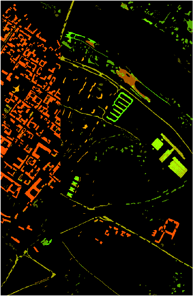
(b)

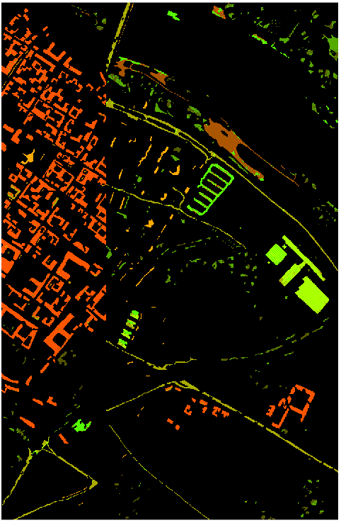
(c)

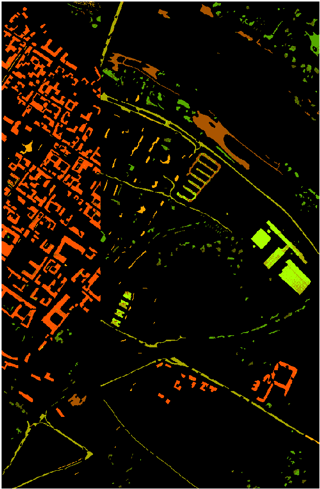
(d)

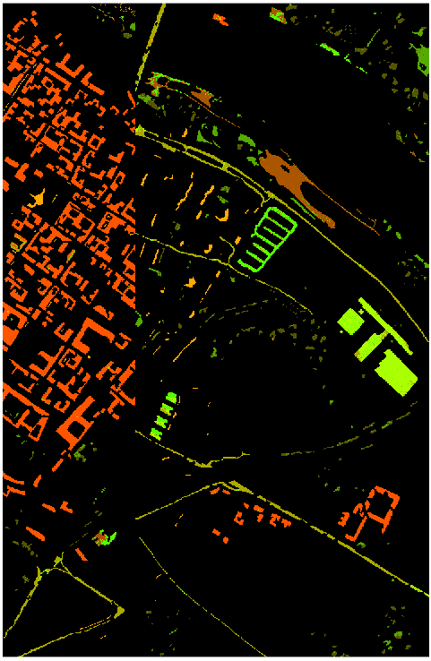
(e)

Figure 3: Label maps on Pavia Centre using 13 training samples per class. (a) ground truth, (b) EMAP-PCA, (c) EMAP-PCA with $500$ synthetic samples per class, (d) EMAP-NWFE, (e) EMAP-NWFE with $500$ synthetic samples per class.

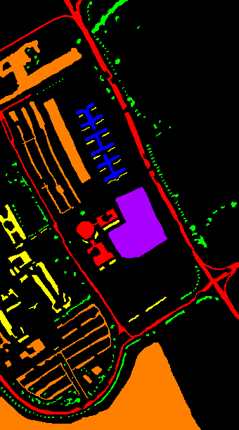
(a)

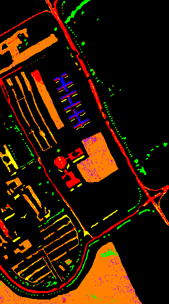
(b)

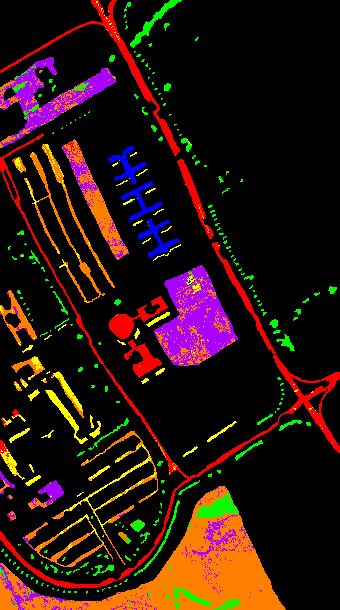
(c)

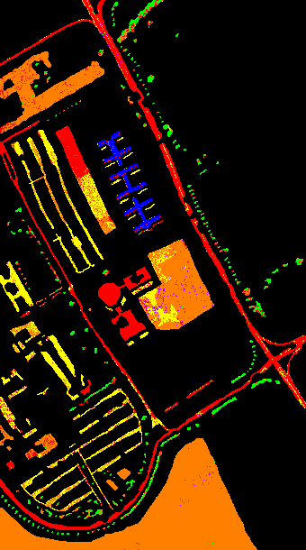
(d)

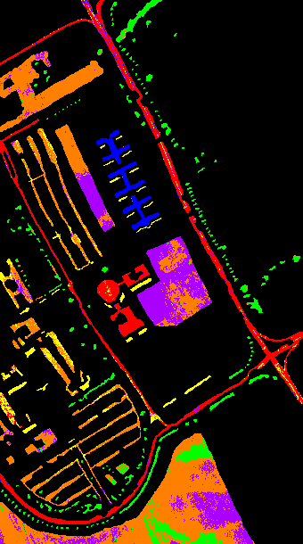
(e)

Figure 4: Label maps on Pavia University using 13 training samples per class. (a) ground truth, (b) EMAP-PCA, (c) EMAP-PCA with $500$ synthetic samples per class, (d) EMAP-NWFE, (e) EMAP-NWFE with $500$ synthetic samples per class.

References

- [1] S. Valero, P. Salembier, and J. Chanussot, “Hyperspectral image representation and processing with binary partition trees,” Image Processing, IEEE Transactions on, vol. 22, no. 4, pp. 1430–1443, 2013.
- [2] J. P. Hoffbeck and D. A. Landgrebe, “Covariance matrix estimation and classification with limited training data,” IEEE Transactions on Pattern Analysis and Machine Intelligence, vol. 18, no. 7, pp. 763–767, 1996.
- [3] S. Tadjudin and D. A. Landgrebe, “Covariance estimation for limited training samples,” in IEEE International Geoscience and Remote Sensing Symposium, vol. 5, pp. 2688–2690, 1998.
- [4] L. Bruzzone, M. Chi, and M. Marconcini, “A novel transductive svm for semisupervised classification of remote-sensing images,” IEEE Transactions on Geoscience and Remote Sensing, vol. 44, no. 11, pp. 3363–3373, 2006.
- [5] M. Chi, R. Feng, and L. Bruzzone, “Classification of hyperspectral remote-sensing data with primal svm for small-sized training dataset problem,” Advances in Space Research, vol. 41, no. 11, pp. 1793–1799, 2008.
- [6] J. Xia, J. Chanussot, P. Du, and X. He, “Rotation-based support vector machine ensemble in classification of hyperspectral data with limited training samples,” IEEE Transactions on Geoscience and Remote Sensing, vol. 54, no. 3, pp. 1519–1531, 2016.
- [7] J. Li, X. Huang, P. Gamba, J. M. Bioucas-Dias, L. Zhang, J. A. Benediktsson, and A. Plaza, “Multiple feature learning for hyperspectral image classification,” IEEE Transactions on Geoscience and Remote Sensing, vol. 53, no. 3, pp. 1592–1606, 2015.
- [8] M. Sofolahan and O. Ersoy, “Summed component analysis for dimensionality reduction and classification,” Tech. Rep. 445, Purdue University, 2013.
- [9] B.-C. Kuo and D. A. Landgrebe, “Nonparametric weighted feature extraction for classification,” IEEE Transactions on Geoscience and Remote Sensing, vol. 42, no. 5, pp. 1096–1105, 2004.
- [10] K. Fukunaga, Introduction to statistical pattern recognition. Academic press, 2013.
- [11] C. Lee and D. A. Landgrebe, “Feature extraction based on decision boundaries,” IEEE Transactions on Pattern Analysis and Machine Intelligence, vol. 15, no. 4, pp. 388–400, 1993.
- [12] T. Castaings, B. Waske, J. Atli Benediktsson, and J. Chanussot, “On the influence of feature reduction for the classification of hyperspectral images based on the extended morphological profile,” International Journal of Remote Sensing, vol. 31, no. 22, pp. 5921–5939, 2010.
- [13] A. Kianisarkaleh and H. Ghassemian, “Nonparametric feature extraction for classification of hyperspectral images with limited training samples,” ISPRS Journal of Photogrammetry and Remote Sensing, vol. 119, pp. 64–78, 2016.
- [14] T. Heimann, P. Mountney, M. John, and R. Ionasec, “Real-time ultrasound transducer localization in fluoroscopy images by transfer learning from synthetic training data,” Medical image analysis, vol. 18, no. 8, pp. 1320–1328, 2014.
- [15] M. Unberath, O. Taubmann, B. Bier, T. Geimer, M. Hell, S. Achenbach, and A. Maier, “Respiratory motion compensation in rotational angiography: Graphical model-based optimization of auto-focus measures,” in Biomedical Imaging (ISBI 2017), 2017 IEEE 14th International Symposium on, pp. 227–230, IEEE, 2017.
- [16] A. A. Davari, E. Aptoula, and B. Yanikoglu, “On the effect of synthetic morphological feature vectors on hyperspectral image classification performance,” in 2015 23nd Signal Processing and Communications Applications Conference (SIU), pp. 653–656, IEEE, 2015.
- [17] I. Goodfellow, J. Pouget-Abadie, M. Mirza, B. Xu, D. Warde-Farley, S. Ozair, A. Courville, and Y. Bengio, “Generative adversarial nets,” in Advances in neural information processing systems, pp. 2672–2680, 2014.
- [18] A. Shrivastava, T. Pfister, O. Tuzel, J. Susskind, W. Wang, and R. Webb, “Learning from simulated and unsupervised images through adversarial training,” arXiv preprint arXiv:1612.07828, 2016.
- [19] M. Dalla Mura, J. Atli Benediktsson, B. Waske, and L. Bruzzone, “Extended profiles with morphological attribute filters for the analysis of hyperspectral data,” International Journal of Remote Sensing, vol. 31, no. 22, pp. 5975–5991, 2010.
- [20] D. Reynolds, “Gaussian mixture models,” in Encyclopedia of Biometrics, pp. 659–663, Springer, 2009.
- [21] G. McLachlan and D. Peel, Finite mixture models. John Wiley & Sons, 2004.
- [22] A. Oliveira-Brochado and F. V. Martins, “Assessing the number of components in mixture models: a review,” tech. rep., Universidade do Porto, Faculdade de Economia do Porto, 2005.
- [23] T. Liu, Y. Gu, X. Jia, J. A. Benediktsson, and J. Chanussot, “Class-specific sparse multiple kernel learning for spectral–spatial hyperspectral image classification,” IEEE Transactions on Geoscience and Remote Sensing, vol. 54, no. 12, p. 7351, 2016.
- [24] L. Breiman, “Random forests,” Machine Learning, vol. 45, pp. 5–32, 2001.
- [25] E. Aptoula, M. C. Ozdemir, and B. Yanikoglu, “Deep learning with attribute profiles for hyperspectral image classification,” IEEE Geoscience and Remote Sensing Letters, 2016.
- [26] C. Tao, H. Pan, Y. Li, and Z. Zou, “Unsupervised spectral-spatial feature learning with stacked sparse autoencoder for hyperspectral imagery classification,” IEEE Geoscience and Remote Sensing Letters, vol. 12, no. 12, pp. 2438–2442, 2015.
- [27] L. Guo, N. Chehata, C. Mallet, and S. Boukir, “Relevance of airborne lidar and multispectral image data for urban scene classification using random forests,” ISPRS Journal of Photogrammetry and Remote Sensing, vol. 66, no. 1, pp. 56–66, 2011.
- [28] M. Dalla Mura, J. A. Benediktsson, B. Waske, and L. Bruzzone, “Morphological attribute profiles for the analysis of very high resolution images,” Geoscience and Remote Sensing, IEEE Transactions on, vol. 48, no. 10, pp. 3747–3762, 2010.
- [29] E. Aptoula, “Hyperspectral image classification with multidimensional attribute profiles,” IEEE Geoscience and Remote Sensing Letters, vol. 12, no. 10, pp. 2031–2035, 2015.
- [30] E. Aptoula, “The impact of multivariate quasi-flat zones on the morphological description of hyperspectral images,” International Journal of Remote Sensing, vol. 35, no. 10, pp. 3482–3498, 2014.
- [31] E. Aptoula, M. Dalla Mura, and S. Lefèvre, “Vector attribute profiles for hyperspectral image classification,” IEEE Transactions on Geoscience and Remote Sensing, vol. 54, no. 6, pp. 3208–3220, 2016.
- [32] V. F. Rodriguez-Galiano, B. Ghimire, J. Rogan, M. Chica-Olmo, and J. P. Rigol-Sanchez, “An assessment of the effectiveness of a random forest classifier for land-cover classification,” ISPRS Journal of Photogrammetry and Remote Sensing, vol. 67, pp. 93–104, 2012.

References

- [1] S. Valero, P. Salembier, and J. Chanussot, “Hyperspectral image representation and processing with binary partition trees,” Image Processing, IEEE Transactions on, vol. 22, no. 4, pp. 1430–1443, 2013.
- [2] J. P. Hoffbeck and D. A. Landgrebe, “Covariance matrix estimation and classification with limited training data,” IEEE Transactions on Pattern Analysis and Machine Intelligence, vol. 18, no. 7, pp. 763–767, 1996.
- [3] S. Tadjudin and D. A. Landgrebe, “Covariance estimation for limited training samples,” in IEEE International Geoscience and Remote Sensing Symposium, vol. 5, pp. 2688–2690, 1998.
- [4] L. Bruzzone, M. Chi, and M. Marconcini, “A novel transductive svm for semisupervised classification of remote-sensing images,” IEEE Transactions on Geoscience and Remote Sensing, vol. 44, no. 11, pp. 3363–3373, 2006.
- [5] M. Chi, R. Feng, and L. Bruzzone, “Classification of hyperspectral remote-sensing data with primal svm for small-sized training dataset problem,” Advances in Space Research, vol. 41, no. 11, pp. 1793–1799, 2008.
- [6] J. Xia, J. Chanussot, P. Du, and X. He, “Rotation-based support vector machine ensemble in classification of hyperspectral data with limited training samples,” IEEE Transactions on Geoscience and Remote Sensing, vol. 54, no. 3, pp. 1519–1531, 2016.
- [7] J. Li, X. Huang, P. Gamba, J. M. Bioucas-Dias, L. Zhang, J. A. Benediktsson, and A. Plaza, “Multiple feature learning for hyperspectral image classification,” IEEE Transactions on Geoscience and Remote Sensing, vol. 53, no. 3, pp. 1592–1606, 2015.
- [8] M. Sofolahan and O. Ersoy, “Summed component analysis for dimensionality reduction and classification,” Tech. Rep. 445, Purdue University, 2013.
- [9] B.-C. Kuo and D. A. Landgrebe, “Nonparametric weighted feature extraction for classification,” IEEE Transactions on Geoscience and Remote Sensing, vol. 42, no. 5, pp. 1096–1105, 2004.
- [10] K. Fukunaga, Introduction to statistical pattern recognition. Academic press, 2013.
- [11] C. Lee and D. A. Landgrebe, “Feature extraction based on decision boundaries,” IEEE Transactions on Pattern Analysis and Machine Intelligence, vol. 15, no. 4, pp. 388–400, 1993.
- [12] T. Castaings, B. Waske, J. Atli Benediktsson, and J. Chanussot, “On the influence of feature reduction for the classification of hyperspectral images based on the extended morphological profile,” International Journal of Remote Sensing, vol. 31, no. 22, pp. 5921–5939, 2010.
- [13] A. Kianisarkaleh and H. Ghassemian, “Nonparametric feature extraction for classification of hyperspectral images with limited training samples,” ISPRS Journal of Photogrammetry and Remote Sensing, vol. 119, pp. 64–78, 2016.
- [14] T. Heimann, P. Mountney, M. John, and R. Ionasec, “Real-time ultrasound transducer localization in fluoroscopy images by transfer learning from synthetic training data,” Medical image analysis, vol. 18, no. 8, pp. 1320–1328, 2014.
- [15] M. Unberath, O. Taubmann, B. Bier, T. Geimer, M. Hell, S. Achenbach, and A. Maier, “Respiratory motion compensation in rotational angiography: Graphical model-based optimization of auto-focus measures,” in Biomedical Imaging (ISBI 2017), 2017 IEEE 14th International Symposium on, pp. 227–230, IEEE, 2017.
- [16] A. A. Davari, E. Aptoula, and B. Yanikoglu, “On the effect of synthetic morphological feature vectors on hyperspectral image classification performance,” in 2015 23nd Signal Processing and Communications Applications Conference (SIU), pp. 653–656, IEEE, 2015.
- [17] I. Goodfellow, J. Pouget-Abadie, M. Mirza, B. Xu, D. Warde-Farley, S. Ozair, A. Courville, and Y. Bengio, “Generative adversarial nets,” in Advances in neural information processing systems, pp. 2672–2680, 2014.
- [18] A. Shrivastava, T. Pfister, O. Tuzel, J. Susskind, W. Wang, and R. Webb, “Learning from simulated and unsupervised images through adversarial training,” arXiv preprint arXiv:1612.07828, 2016.
- [19] M. Dalla Mura, J. Atli Benediktsson, B. Waske, and L. Bruzzone, “Extended profiles with morphological attribute filters for the analysis of hyperspectral data,” International Journal of Remote Sensing, vol. 31, no. 22, pp. 5975–5991, 2010.
- [20] D. Reynolds, “Gaussian mixture models,” in Encyclopedia of Biometrics, pp. 659–663, Springer, 2009.
- [21] G. McLachlan and D. Peel, Finite mixture models. John Wiley & Sons, 2004.
- [22] A. Oliveira-Brochado and F. V. Martins, “Assessing the number of components in mixture models: a review,” tech. rep., Universidade do Porto, Faculdade de Economia do Porto, 2005.
- [23] T. Liu, Y. Gu, X. Jia, J. A. Benediktsson, and J. Chanussot, “Class-specific sparse multiple kernel learning for spectral–spatial hyperspectral image classification,” IEEE Transactions on Geoscience and Remote Sensing, vol. 54, no. 12, p. 7351, 2016.
- [24] L. Breiman, “Random forests,” Machine Learning, vol. 45, pp. 5–32, 2001.
- [25] E. Aptoula, M. C. Ozdemir, and B. Yanikoglu, “Deep learning with attribute profiles for hyperspectral image classification,” IEEE Geoscience and Remote Sensing Letters, 2016.
- [26] C. Tao, H. Pan, Y. Li, and Z. Zou, “Unsupervised spectral-spatial feature learning with stacked sparse autoencoder for hyperspectral imagery classification,” IEEE Geoscience and Remote Sensing Letters, vol. 12, no. 12, pp. 2438–2442, 2015.
- [27] L. Guo, N. Chehata, C. Mallet, and S. Boukir, “Relevance of airborne lidar and multispectral image data for urban scene classification using random forests,” ISPRS Journal of Photogrammetry and Remote Sensing, vol. 66, no. 1, pp. 56–66, 2011.
- [28] M. Dalla Mura, J. A. Benediktsson, B. Waske, and L. Bruzzone, “Morphological attribute profiles for the analysis of very high resolution images,” Geoscience and Remote Sensing, IEEE Transactions on, vol. 48, no. 10, pp. 3747–3762, 2010.
- [29] E. Aptoula, “Hyperspectral image classification with multidimensional attribute profiles,” IEEE Geoscience and Remote Sensing Letters, vol. 12, no. 10, pp. 2031–2035, 2015.
- [30] E. Aptoula, “The impact of multivariate quasi-flat zones on the morphological description of hyperspectral images,” International Journal of Remote Sensing, vol. 35, no. 10, pp. 3482–3498, 2014.
- [31] E. Aptoula, M. Dalla Mura, and S. Lefèvre, “Vector attribute profiles for hyperspectral image classification,” IEEE Transactions on Geoscience and Remote Sensing, vol. 54, no. 6, pp. 3208–3220, 2016.
- [32] V. F. Rodriguez-Galiano, B. Ghimire, J. Rogan, M. Chica-Olmo, and J. P. Rigol-Sanchez, “An assessment of the effectiveness of a random forest classifier for land-cover classification,” ISPRS Journal of Photogrammetry and Remote Sensing, vol. 67, pp. 93–104, 2012.