Approximation of Sojourn Times of Gaussian Processes

Abstract: We investigate the tail asymptotic behavior of the sojourn time for a large class of centered Gaussian processes $X$, in both continuous- and discrete-time framework. All results obtained here are new for the discrete-time case. In the continuous-time case, we complement the investigations of [1, 2] for non-stationary $X$. A by-product of our investigation is a new representation of Pickands constant which is important for Monte-Carlo simulations and yields a sharp lower bound for Pickands constant.

Key Words: sojourn time; occupation time; exact asymptotics; Gaussian process; locally stationary processes.

AMS Classification: Primary 60G15; secondary 60G70

1. Introduction

Let $X(t),t\in\mathbb{R}$ be a centered Gaussian process with variance function $\sigma^{2}$, correlation function $\rho$ and continuous trajectories. By

$$L_{u}[a,b]:=\int_{a}^{b}\mathbb{I}_{u}\left(X(t)\right)\text{\rm d}t$$

we define the sojourn time spent above a fixed level $u$ by the process $X$ on the interval $[a,b]$, where $\mathbb{I}_{u}\left(x\right):=\mathbb{I}\left(x>u\right)$.

In a series of papers culminating in [3], S. Berman derived results on the tail asymptotic behaviour of $L_{u}[a,b]$, as $u\to\infty$. The sojourn time approach to tackle this problem consists in finding explicitly an appropriate scaling function $v(u)$ such that for some function $C(x)>0,x\geq 0$

(1.1) $$\mathbb{P}\left\{L_{u}[a,b]>x/v(u)\right\} \sim C(x)\mathbb{P}\left\{L_{u}[a,b]>0\right\}=C(x)\mathbb{P}\left\{\sup_{t\in[a,b]}X(t)>u\right\},\quad u\to\infty$$

for any $x\geq 0$ a continuity point of $C(\cdot)$. In our notation $\sim$ stands for asymptotic equivalence of two functions as the argument tends to 0 or $\infty$. Additional inside of this approach is the explicit calculation of the exact asymptotics of $\mathbb{P}\left\{\sup_{t\in[a,b]}X(t)>u\right\}$ as $u\to\infty$. For example, as shown in several works of Berman and Pickands (see e.g., [4, 3, 5]) for $X$ a centered stationary Gaussian process the asymptotic tail behaviour of $v(u)L_{u}([a,b])$ and that of $\sup_{t\in[a,b]}X(t)$ can be studied under appropriate assumptions on the correlation function $\rho$. Pickands’ assumption for $X$ stationary with unit variance function reads

(1.2) $$1-\rho(t)\sim\left\lvert t\right\rvert^{\alpha},\ t\to 0\quad\textrm{and}\quad\rho(t)<1,\ \forall\,t\not=0,$$

where $\alpha\in(0,2]$. Under (1.2) in view of [5] (see also [6]) taking the scaling function $v(u)=u^{2/\alpha}$ we have (consider for simplicity $[a,b]=[0,T],T>0$)

(1.3) $$\mathbb{P}\left\{\sup_{t\in[0,T]}X(t)>u\right\}\sim T\mathcal{H}_{\alpha}v(u)\mathbb{P}\left\{X(0)>u\right\},\quad u\to\infty,$$

where $\mathcal{H}_{\alpha}$ is the Pickands constant given by

$$\mathcal{H}_{\alpha}=\lim_{S\to\infty}S^{-1}\mathcal{H}_{\alpha}([0,S])\in(0,\infty),$$

with

(1.4) $$\mathcal{H}_{\alpha}([0,S])=\mathbb{E}\left\{\sup_{t\in[0,S]}e^{W_{\alpha}(t)}\right\},\quad W_{\alpha}(t):=\sqrt{2}B_{\alpha}(t)-\left\lvert t\right\rvert^{\alpha}$$

and $B_{\alpha}$ is a standard fractional Brownian motion (fBm) with Hurst index $\alpha/2\in(0,1]$. A refinement of (1.3) is given in [3][Theorem 3.3.1]. Namely, (1.1) holds with

$$C(x)=\widetilde{\mathcal{B}}_{\alpha}(x)/\mathcal{H}_{\alpha}$$

for any $x>0$ a continuity point of $\widetilde{\mathcal{B}}_{\alpha}(\cdot)$. Here $\widetilde{\mathcal{B}}_{\alpha}(x)=\int_{x}^{\infty}\frac{1}{y}\,\text{\rm d}\mathcal{G}_{\alpha}(y)\in(0,\infty),$ with

(1.5) $$\mathcal{G}_{\alpha}(x)=\mathbb{P}\left\{\int_{\mathbb{R}}\mathbb{I}_{0}\left(W_{\alpha}(s)+\mathcal{E}\right)\text{\rm d}s\leq x\right\},$$

where $\mathcal{E}$ is a unit exponential random variable independent of $W_{\alpha}$. Furthermore, as shown in [3][Theorem 10.5.1]

(1.6) $$\widetilde{\mathcal{B}}_{\alpha}(0)=\lim_{x\downarrow 0}\int_{x}^{\infty}\frac{1}{y}\,\text{\rm d}G_{\alpha}(y)=\mathcal{H}_{\alpha}\,.$$

We note that the only known values of Pickands constants are $\mathcal{H}_{1}=1$ and $\mathcal{H}_{2}=\frac{1}{\sqrt{\pi}}$ and both (1.4) and (1.6) are not tractable for simulations. In Theorem 1.1 we present an interesting formula for $\mathcal{H}_{\alpha}$, which is a consequence of Berman’s theory on extremes of random processes. We believe that this new formula is of particular interest for simulations, since it is given as an expectation, see [7, 8, 9, 10, 11] for alternative formulas. Another advantage of this new formula is that it implies the uniformly (with respect to $\alpha$) sharpest lower bound for the Pickands constant available in the literature so far. Next, let $\Gamma(\cdot)$ stands for Euler Gamma function.

Theorem 1.1.

For $\alpha\in(0,2]$ we have

(1.7) $$\mathcal{H}_{\alpha}=\mathbb{E}\left\{\frac{1}{\int_{\mathbb{R}}\mathbb{I}_{0}\left(W_{\alpha}(s)+\mathcal{E}\right)ds}\right\}\geq\frac{\Gamma(1/\alpha)}{4\Gamma(2/\alpha)}.$$

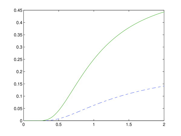
Figure 1. Solid line: lower bound (1.7), dashed line: lower bound (1.8)

Interestingly, the same lower bound for $\mathcal{H}_{\alpha}$ as derived in Theorem 1.1 was obtained heuristically in [12][J20a,J20b]. The above finding uniformly improves the result of [13] (see also [14]):

(1.8) $$\mathcal{H}_{\alpha}\geq\frac{4^{-\frac{1}{\alpha}-1}}{\Gamma(1/\alpha+1)};$$

see Fig. 1. We refer to [15] for the proof that $\mathcal{H}_{\alpha}\geq\frac{(1.1527)^{1/\alpha}}{\Gamma(1/\alpha)}$ for $\alpha$ sufficiently close to $0$, which subverted an opened for long time hypothesis that $\mathcal{H}_{\alpha}=\frac{1}{\Gamma(1/\alpha)}$. Other estimates for Pickands constants can be found in e.g., [16] and [7].

The main interest of this contribution is the investigation of the tail asymptotics of $L_{u}[a,b]$ and its discrete counterpart.
Our method here is completely different from that of Berman. Namely, in this paper we developed the uniform double-sum method for the sojourn time functional. Interestingly, this approach leads to a new representation of Berman’s constants $\widetilde{\mathcal{B}}_{\alpha}(x)$; see Section 2 where the asymptotics for the tail distribution of sojourns of locally-stationary Gaussian processes was derived and compared with the classical results of Berman.

Our main findings in this paper can be summarized as follows: for both locally-stationary Gaussian processes and general non-stationary Gaussian processes with variance maximal at some unique point, we show that (1.1) holds for almost all $x$ and moreover, we calculate explicitly $C(x)$ and give the appropriate scaling function $v$. Our results are new for non-stationary Gaussian processes, and agree with those of Berman for the locally stationary ones. In particular, all results are new for the discrete setup introduced in the next section.

Brief organisation of the rest of the paper: In Section 2 we derive the tail asymptotics of sojourn time for locally stationary Gaussian processes. Corresponding results for general non-stationary Gaussian processes are then presented in Section 3. All the proofs are displayed in Section 4 whereas few technical results are included in Section 5.

2. Sojourns of Locally Stationary Gaussian Processes

In this section we analyze sojourns for the class of locally stationary Gaussian processes, introduced by Berman in [3], see also [17, 18, 19, 20, 21, 22]. Specifically, let $X(t),t\in[0,T]$ be a centered Gaussian process with unit variance and correlation function $\rho$ satisfying

(2.1) $$\lim_{\epsilon\to 0}\sup_{t,t+s\in[0,T],|s|<\epsilon}\left\lvert\frac{1-\rho(t,t+s)}{K(\left\lvert s\right\rvert)}-H(t)\right\rvert=0,$$

where $H$ is a continuous positive function on $[0,T]$ and $K$ is a regularly varying function at 0 with index $\alpha\in(0,2]$. In the following let $v$ be the asymptotically unique function (which exists, see [3]) such that $\lim_{u\to\infty}v(u)=\infty$ and

(2.2) $$\lim_{u\to\infty}u^{2}K(1/v(u))=1.$$

We shall investigate the tail asymptotics of $L_{u}^{*}[0,T]:=v(u)L_{u}[0,T]$. Given some $\eta>0$ we define the discrete counterpart of $L_{u}^{*}[a,b]$ as

$$L_{\eta,u}^{*}[a,b]:=v(u)\int_{a}^{b}\mathbb{I}_{u}\left(X(t)\right)\mu_{\eta_{u}}(\text{\rm d}t)=\eta\sum_{t\in(\eta_{u}\mathbb{Z})\cap[a,b]}\mathbb{I}_{u}\left(X(t)\right),$$

where $\eta_{u}=\eta/v(u)$ and $\mu_{c}(dt)/c$ denotes the counting measure on $c\mathbb{Z}$. In the sequel we interpret $0\mathbb{Z}$ as $\mathbb{R}$ and $\mu_{0}$ as the Lebesgue measure on $\mathbb{R}$. Since $\mu_{c}$ converges to the Lebesgue measure $\mu_{0}$ on $\mathbb{R}$ as $c\to 0$, with this convention we set

$$L_{0,u}^{*}[a,b]:=L_{u}^{*}[a,b]=v(u)L_{u}[a,b].$$

In order to state our first result, define for any $\lambda>0,\eta\geq 0,x\in[0,\mu_{\eta}([0,S]))$

(2.3) $$\mathcal{B}_{\alpha,\lambda}^{\eta}(S,x):=\int_{\mathbb{R}}\mathbb{P}\left\{\int_{0}^{S}\mathbb{I}_{0}\left(W_{\alpha}(\lambda^{1/\alpha}s)+z\right)\mu_{\eta}(\text{\rm d}s)>x\right\}e^{-z}\text{\rm d}z,$$

where $W_{\alpha}$ is defined in (1.4). Further, for any $x\geq 0$ set

(2.4) $$\mathcal{B}_{\alpha}^{\eta,H}(x):=\lim_{S\to\infty}\frac{\int_{0}^{T}\mathcal{B}_{\alpha,H(t)}^{\eta}(S,x)\text{\rm d}t}{S},\quad\mathcal{B}_{\alpha}^{\eta}(x):=\lim_{S\to\infty}S^{-1}\mathcal{B}_{\alpha,1}^{\eta}(S,x).$$

Hereafter, when we mention that $x$ is a continuity point for some function $f$ we also assume that $f(x)>0$.

Next we state our first result. The case $\eta>0$ is new, whereas for the case $\eta=0$ we retrieve the result of Berman, however the asymptotic constant (pre-factor) is given in a different form than in the original Berman’s result, see e.g. [4], which is due to a different technique applied here.

Theorem 2.1.

Let $X(t),t\in[0,T]$ be a centered, sample path continuous Gaussian process with unit variance and correlation function satisfying assumption (2.1). If further $\rho(s,t)<1$ for all $s,t\in[0,T],s\neq t$, then for any $x>0$ a continuity point of $\mathcal{B}_{\alpha}^{\eta,H}(\cdot)$ and for $x=0$ we have

(2.5) $$\mathbb{P}\left\{L_{\eta,u}^{*}[0,T]>x\right\}\sim\mathcal{B}_{\alpha}^{\eta,H}(x)v(u)\mathbb{P}\left\{X(0)>u\right\},\quad u\to\infty,$$

where $v(u)$ is given in (2.2) and $\mathcal{B}_{\alpha}^{\eta,H}(\cdot)$ defined in (2.4) is positive and finite for any $x,\eta\geq 0$.

Remark 2.2.

i) If $X(t),t\in[0,T]$ is a centered, stationary, sample path continuous Gaussian process with unit variance function and its correlation function $\rho$ satisfies Pickands condition (1.2), then $X$ is locally stationary with function $H(t)\equiv 1,t\in[0,T]$. For such $H$ we have that $\mathcal{B}_{\alpha}^{\eta,H}(x)=T\mathcal{B}_{\alpha}^{\eta}(x)$.
ii) For $\eta=0$, by [3][Theorem 3.3.1] and (2.5) we have

$$\mathcal{B}_{\alpha}^{0}(x)=\widetilde{\mathcal{B}}_{\alpha}(x)$$

for all continuity points of $\widetilde{\mathcal{B}}_{\alpha}(\cdot)$ (since both $\mathcal{B}_{\alpha}^{0}(\cdot)$ and $\widetilde{\mathcal{B}}_{\alpha}(\cdot)$ are monotone non-increasing).

3. Sojourns of Non-Stationary Gaussian Processes

In this section we analyze sojourns of non-stationary centered Gaussian processes. Suppose that $X(t),t\in[-T,T]$ is a centered Gaussian process with continuous sample paths. Tractable assumptions on both variance $\sigma^{2}(t)=Var(X(t))$ and correlation function $\rho(s,t)$, adopted from a vast literature on the asymptotic analysis of supremum of non-stationary Gaussian processes, see e.g., [23, 24, 25, 2, 26, 1, 27, 6, 19, 28], are as follows:

• For some $T>0$

  $$t_{0}={\rm argmax}_{t\in[-T,T]}\sigma(t)$$

  is unique. For notational simplicity we assume further that $t_{0}=0$ and $\sigma(t_{0})=1.$

• For some $\alpha\in(0,2]$ we have

  $$1-\rho(s,t)\sim\left\lvert t-s\right\rvert^{\alpha},\qquad s,t\to t_{0}.$$

• For some positive constants $b,\beta$

  $$1-\sigma(t)\sim b\left\lvert t\right\rvert^{\beta},\qquad t\to t_{0}.$$

Under the assumptions A0-A1, if further

$$\lim_{s,t\to 0,s\neq t}\frac{\left\lvert\sigma(s)-\sigma(t)\right\rvert}{\mathbb{E}\left\{(X(s)-X(t))^{2}\right\}}=0$$

in view of [1][Theorem 6.1] we have

$$\lim_{u\to\infty}\frac{\int_{0}^{x}y\text{\rm d}\mathbb{P}\left\{L_{u}^{*}[-T,T]\leq y\right\}}{\mathbb{E}\left\{L_{u}^{*}[-T,T]\right\}}=\mathcal{G}_{\alpha}(x)$$

for any continuity point $x$ of $\mathcal{G}_{\alpha}$ defined in (1.5).
See also [2] for another result shown under A0, A2 assuming further that

$$\lim_{t\to 0}\frac{\mathbb{E}\left\{(X(t)-X(0))^{2}\right\}}{1-\sigma(t)}=0.$$

Under the assumptions A0-A2 we shall derive the tail asymptotics of $L_{\eta,u}^{*}[-T,T]$, where we chose the scaling function $v(u)$ as follows

(3.1) $$v(u)=u^{2/\min(\alpha,\beta)}.$$

As in the case of Piterbarg’s result for $\sup_{t\in[-T,T]}X(t)$ (see [6]), if $\alpha=\beta$ in the asymptotic results a new constant $\mathcal{P}_{\alpha}^{b,\eta}$ appears, which is defined for any $b>0$ by

(3.2) $$\mathcal{P}^{b,\eta}_{\alpha}(x):=\int_{\mathbb{R}}\mathbb{P}\left\{\int_{\mathbb{R}}\mathbb{I}_{0}\left(W_{\alpha}(s)-b\left\lvert s\right\rvert^{\alpha}+z\right)\mu_{\eta}(ds)>x\right\}e^{-z}\text{\rm d}z.$$

Additionally, for $\eta>0$ we set

(3.5) $$\mathcal{T}^{b,\eta}_{\beta}(x)=\left\{\begin{array}[]{ll}1&\mbox{if $x\in[0,\eta)$}\\[14.22636pt] e^{-b(k\eta)^{\beta}}&\mbox{if $x\in[(2k-1)\eta,(2k+1)\eta),k\in\mathbb{N}$}\end{array}\right.$$

and for $\eta=0$, $x\geq 0$ let $\mathcal{T}^{b,0}_{\beta}(x)=e^{-b(\frac{x}{2})^{\beta}}.$

We present next the main result of this section.

Theorem 3.1.

Let $X$ be a centered Gaussian process satisfying A0-A2, $\eta\geq 0$ and $v(u)=u^{2/\min(\alpha,\beta)}$.
i) If $\alpha<\beta$, then for any $x>0$ a continuity point of $\mathcal{B}_{\alpha}^{\eta}(\cdot)$ and $x=0$

(3.6) $$\mathbb{P}\left\{L_{\eta,u}^{*}[-T,T]>x\right\}\ \sim\ 2b^{-1/\beta}\Gamma(1/\beta+1)\mathcal{B}_{\alpha}^{\eta}(x)u^{2/\alpha-2/\beta}\mathbb{P}\left\{X(0)>u\right\},\quad u\to\infty.$$

ii) If $\alpha=\beta$, then for any $x>0$ a continuity point of $\mathcal{P}_{\alpha}^{b,\eta}(\cdot)$ and $x=0$

(3.7) $$\mathbb{P}\left\{L_{\eta,u}^{*}[-T,T]>x\right\}\ \sim\ \mathcal{P}^{b,\eta}_{\alpha}(x)\mathbb{P}\left\{X(0)>u\right\},\quad u\to\infty.$$

iii) If $\beta<\alpha$, then for any $x>0$ a continuity point of $\mathcal{T}^{b,\eta}_{\beta}(\cdot)$ and $x=0$

(3.8) $$\mathbb{P}\left\{L_{\eta,u}^{*}[-T,T]>x\right\}\ \sim\ \mathcal{T}^{b,\eta}_{\beta}(x)\mathbb{P}\left\{X(0)>u\right\},\quad u\to\infty.$$

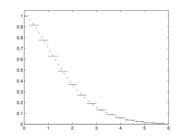
Figure 2. Graph of $\mathcal{T}_{1.5}^{1,\eta}(\cdot)$. Solid line: $\eta=0.2$, dashed line: $\eta=0$.

Remark 3.2.

i) If $\eta=x=0$, then $\mathcal{P}^{b,0}_{\alpha}(0)=\mathcal{P}_{\alpha}^{b}$. Indeed, for any $b>0$ we have

$$\mathcal{P}^{b,0}_{\alpha}(0) = \int_{\mathbb{R}}\mathbb{P}\left\{\int_{s\in\mathbb{R}}\mathbb{I}_{0}\left(W_{\alpha}(s)-b\left\lvert s\right\rvert^{\alpha}+z\right)\text{\rm d}s>0\right\}e^{-z}\text{\rm d}z$$

$$= \int_{\mathbb{R}}\mathbb{P}\left\{\sup_{s\in\mathbb{R}}\Bigl{(}W_{\alpha}(s)-b\left\lvert s\right\rvert^{\alpha}+z\Bigr{)}>0\right\}e^{-z}\text{\rm d}z$$

$$= \mathbb{E}\left\{\sup_{s\in\mathbb{R}}e^{W_{\alpha}(s)-b\left\lvert s\right\rvert^{\alpha}}\right\}=:\mathcal{P}_{\alpha}^{b}.$$

In the literature, $\mathcal{P}_{\alpha}^{b}$ is referred to as Piterbarg constant, see [24, 29, 30, 31] for related constants and basic properties.
ii) If $t_{0}\in\{-T,T\}$ in A0, then Theorem 3.1 still holds subject to appropriate change of the constants in the asymptotics. Specifically, if $\alpha<\beta$, (3.6) holds with the constant $2$ removed from the expression. If $\alpha=\beta$, then $\mathcal{P}^{b,\eta}_{\alpha}(x)$ in (3.7) has to be changed to

$$\int_{\mathbb{R}}\mathbb{P}\left\{\int_{0}^{\infty}\mathbb{I}_{0}\left(W_{\alpha}(s)-b\left\lvert s\right\rvert^{\alpha}+z\right)\mu_{\eta}(\text{\rm d}s)>x\right\}e^{-z}\text{\rm d}z.$$

If $\alpha>\beta$, then in (3.8) $\mathcal{T}^{b,\eta}_{\beta}(x)$ has to be substituted by $e^{-bx^{\beta}},x\geq 0$ for $\eta=0$, and $e^{-b(k\eta)^{\beta}}$ if $x\in[k\eta,(k+1)\eta),k\in\{0\}\cup\mathbb{N}$ for $\eta>0$.

4. Proofs

Below $\lfloor x\rfloor$ stands for the integer part of $x$ and $\lceil x\rceil$ is the smallest integer not less than $x$. Further $\Psi$ is the survival function of an $N(0,1)$ random variable.

Proof of Theorem 1.1 Since $W_{\alpha}$ has almost surely continuous trajectories with $W_{\alpha}(0)=0$ and $\mathcal{E}>0$ almost surely, then $I_{\alpha}=\int_{\mathbb{R}}\mathbb{I}_{0}\left(W_{\alpha}(s)+\mathcal{E}\right)ds>0$ almost surely. Consequently, by the definition of Pickands constant in (1.6) and the monotone convergence theorem we obtain

$$\mathcal{H}_{\alpha}=\lim_{x\downarrow 0}\int_{x}^{\infty}\frac{1}{y}\,\text{\rm d}\mathcal{G}_{\alpha}(y)=\mathbb{E}\left\{\frac{1}{{I}_{\alpha}}\right\}\in(0,\infty).$$

Hence by Jensen’s inequality we have

$$\mathbb{E}\left\{\frac{1}{{I}_{\alpha}}\right\} \geq \frac{1}{\mathbb{E}\left\{{I}_{\alpha}\right\}}.$$

Further, we have

$$\mathbb{E}\left\{I_{\alpha}\right\} = \int_{\mathbb{R}}\mathbb{P}\left\{W_{\alpha}(t)+\mathcal{E}>0\right\}\,\text{\rm d}t$$

$$= 2\int_{0}^{\infty}\mathbb{P}\left\{W_{\alpha}(t)+\mathcal{E}>0\right\}\,\text{\rm d}t$$

$$= 2\int_{0}^{\infty}\mathbb{P}\left\{\sqrt{2t^{\alpha}}B_{\alpha}(1)-t^{\alpha}+\mathcal{E}>0\right\}\,\text{\rm d}t$$

$$= 4\int_{0}^{\infty}\mathbb{P}\left\{B_{\alpha}(1)>\sqrt{\frac{t^{\alpha}}{2}}\right\}\,\text{\rm d}t$$

$$= 4\int_{0}^{\infty}\mathbb{P}\left\{\max(0,B_{\alpha}(1))>\sqrt{\frac{t^{\alpha}}{2}}\right\}\,\text{\rm d}t$$

$$= 4\mathbb{E}\left\{2^{1/\alpha}({\max(0,B_{\alpha}(1))})^{2/\alpha}\right\}$$

$$= \frac{4^{1/\alpha+1/2}}{\sqrt{\pi}}\Gamma(1/\alpha+1/2),$$

where in (4) we used Lemma 5.4 from Appendix. Thus the proof is complete. $\Box$

Proof of Theorem 2.1 Let $S>1$ be a positive constant. Define $S_{0}=S,S_{\eta}=\eta\lfloor S\rfloor$ for $\eta>0$ and set further

$$\Delta_{k}=[kS_{\eta,u},(k+1)S_{\eta,u}],\quad k=0,\ldots,N_{u},$$

where $S_{\eta,u}=S_{\eta}/v(u)$ and $N_{u}=\lfloor T/S_{\eta,u}\rfloor$. We have for all $u$ positive and $x\geq 0$

(4.2) $$I_{1}(u)\leq\mathbb{P}\left\{L_{\eta,u}^{*}[0,T]>x\right\}\leq I_{2}(u),$$

where

$$I_{1}(u)=\sum_{k=0}^{N_{u}-1}\mathbb{P}\left\{L_{\eta,u}^{*}\Delta_{k}>x\right\}-\sum_{0\leq i<k\leq N_{u}-1}q_{i,k}(u),$$

$$I_{2}(u)=\sum_{k=0}^{N_{u}}\mathbb{P}\left\{L_{\eta,u}^{*}\Delta_{k}>x\right\}+\sum_{0\leq i<k\leq N_{u}}q_{i,k}(u),$$

with

$$q_{i,k}(u)=\mathbb{P}\left\{\sup_{t\in\Delta_{i}}X(t)>u,\sup_{t\in\Delta_{k}}X(t)>u\right\}.$$

We first show that, as $u\to\infty$ and then $S\to\infty$, the first sum in $I_{1}$ is asymptotically equivalent to $v(u)\Psi(u)$ and the double sum is negligible with respect to the former one.
For any $x\geq 0$ and $t\in[0,T]$, put

$$F_{u}(t,x)=\Psi^{-1}(u)\mathbb{P}\left\{v(u)\int_{0}^{S_{\eta,u}}\mathbb{I}_{u}\left(X(t+s)\right)\mu_{\eta_{u}}(\text{\rm d}s)>x\right\}.$$

According to (2.1), we choose $\varepsilon$ small enough such that

(4.3) $$1-\rho(s,t)\leq 2\overline{h}K(\left\lvert t-s\right\rvert)\leq 1,\quad\forall s,t\in[0,T],\left\lvert t-s\right\rvert\leq\varepsilon$$

with $\overline{h}=\max_{t\in[0,T]}H(t)$. Let $Y$ be a centered stationary Gaussian process with continuous trajectories, unit variance function and covariance function satisfying

$$1-\mathrm{Cov}(Y(t),Y(t+s))\sim 4\overline{h}K(\left\lvert s\right\rvert),\quad s\to 0.$$

The existence of such a Gaussian process is guaranteed by the Assertion in [32][p.265] and follows from [33, 34]. Consequently, by Slepian lemma and [30][Lemma 5.1] for any $\eta\geq 0$ and sufficiently large $u$

(4.4) $$\sup_{t\in[0,T]}F_{u}(t,x) \leq \Psi^{-1}(u)\sup_{t\in[0,T]}\mathbb{P}\left\{\sup_{s\in[0,S_{\eta,u}]}X(t+s)>u\right\}$$

$$\leq \Psi^{-1}(u)\mathbb{P}\left\{\sup_{s\in[0,S_{\eta,u}]}Y(s)>u\right\}$$

$$\leq 2\lceil(4{\overline{h}})^{1/\alpha}S_{\eta}\rceil\mathcal{H}_{\alpha}([0,1]),$$

where $\mathcal{H}_{\alpha}(\cdot)$ is defined in (1.4). Therefore,

$$\left\lvert\frac{1}{S_{\eta}}\int_{0}^{T}\frac{1}{\Psi(u)}\mathbb{P}\left\{L_{\eta,u}^{*}[t,t+S_{\eta,u}]>x\right\}\mu_{S_{\eta,u}}(\text{\rm d}t)-\frac{1}{\Psi(u)v(u)}\sum_{k=0}^{N_{u}-1}\mathbb{P}\left\{L_{\eta,u}^{*}\Delta_{k}>x\right\}\right\rvert$$

$$\leq \frac{1}{v(u)}\sup_{t\in[0,T]}F_{u}(t,x)\rightarrow 0$$

as $u\to\infty$ implying

$$\frac{1}{\Psi(u)v(u)}\sum_{k=0}^{N_{u}-1}\mathbb{P}\left\{L_{\eta,u}^{*}\Delta_{k}>x\right\}\sim\frac{1}{S_{\eta}}\int_{0}^{T}F_{u}(t,x)\mu_{S_{\eta,u}}(\text{\rm d}t).$$

Let $x_{0}\in(0,\mu_{\eta}([0,S_{\eta}]))$ be a continuity point of $\int_{0}^{T}\mathcal{B}_{\alpha,H(t)}^{\eta}(S_{\eta},x)dt$, then

$$\lim_{\varepsilon_{0}\to 0}\int_{0}^{T}[\mathcal{B}_{\alpha,H(t)}^{\eta}(S_{\eta},x_{0}+\varepsilon_{0})-\mathcal{B}_{\alpha,H(t)}^{\eta}(S_{\eta},x_{0}-\varepsilon_{0})]\text{\rm d}t=0.$$

Application of the dominated convergence theorem with Lemma 5.2 in Appendix yields

$$\int_{0}^{T}[\mathcal{B}_{\alpha,H(t)}^{\eta}(S_{\eta},x_{0}+)-\mathcal{B}_{\alpha,H(t)}^{\eta}(S_{\eta},x_{0}-)]\text{\rm d}t=0.$$

Since $\mathcal{B}_{\alpha,H(t)}^{\eta}(S_{\eta},x)$ is monotone in $x$ for each $t\in[0,T]$, it follows that $x_{0}$ is a continuity point for any $t\in[0,T]\setminus B$, where $B$ is some subset of $[0,T]$ with Lebesgue measure $0$. Next, by Lemma 5.1-i), for any $t_{u}$ such that $\lim_{u\to\infty}t_{u}=t_{0}\in[0,T]\setminus B$

(4.5) $$\lim_{u\to\infty}F_{u}(t_{u},x_{0})=\mathcal{B}_{\alpha,H(t_{0})}^{\eta}(S_{\eta},x_{0}).$$

By (4.4) for sufficiently large $u_{0}$, $F_{u}(\cdot,x_{0}),u\geq u_{0}$ is uniformly bounded on $[0,T]$. Consequently, [35][Lemma 9.3] implies

(4.6) $$\lim_{u\to\infty}\frac{1}{\Psi(u)v(u)}\sum_{k=0}^{N_{u}-1}\mathbb{P}\left\{L_{\eta,u}^{*}\Delta_{k}>x_{0}\right\} = \lim_{u\to\infty}\frac{1}{S_{\eta}}\int_{0}^{T}F_{u}(t,x_{0})\mu_{S_{\eta,u}}(\text{\rm d}t)$$

$$= \frac{1}{S_{\eta}}\int_{0}^{T}\mathcal{B}_{\alpha,H(t)}^{\eta}(S_{\eta},x_{0})\text{\rm d}t.$$

Further, by Lemma 5.1-i), (4.5) is also valid for $x_{0}=0$. Therefore, (4.6) holds for $x_{0}=0$ and for any $x_{0}\in(0,\mu_{\eta}([0,S_{\eta}]))$ a continuity point of $\int_{0}^{T}\mathcal{B}_{\alpha,H(t)}^{\eta}(S_{\eta},x)dt$.

Define

$$A_{\varepsilon}=\{(i,k):1\leq i+1<k\leq N_{u}-1,k+1-i\leq\lfloor\varepsilon/S_{\eta,u}\rfloor\},$$

$$B_{\varepsilon}=\{(i,k):1\leq i+1<k\leq N_{u}-1,k+1-i>\lfloor\varepsilon/S_{\eta,u}\rfloor\}.$$

Then

(4.7) $$\sum_{0\leq i<k\leq N_{u}-1}q_{i,k}(u)\leq\sum_{0\leq i\leq N_{u}-1}q_{i,i+1}(u)+\sum_{(i,k)\in A_{\varepsilon}}q_{i,k}(u)+\sum_{(i,k)\in B_{\varepsilon}}q_{i,k}(u).$$

Since $\rho(s,t)<1$ for all $s,t\in[0,T],s\neq t$, with a similar argument as used in the proof of Theorem 4 in [13]

(4.8) $$\limsup_{u\to\infty}\frac{1}{v(u)\Psi(u)}\sum_{(i,k)\in B_{\varepsilon}}q_{i,k}(u)=0$$

holds. In view of Lemma 5.3, for large enough $u$

$$\sum_{(i,k)\in A_{\varepsilon}}q_{i,k}(u)\leq 2\lceil(16\overline{h})^{1/\alpha}\rceil^{2}\lceil S_{\eta}\rceil^{2}H_{\alpha}^{2}([0,1])\Psi(u)N_{u}\sum_{k=1}^{\infty}\exp(-\frac{1}{16}\underline{h}\left\lvert kS_{\eta}\right\rvert^{\alpha/2}).$$

Since $\lim_{S\to\infty}e^{S}\sum_{k=1}^{\infty}e^{-Sk^{\alpha/2}}<2$, then for sufficiently large $S$

(4.9) $$\limsup_{u\to\infty}\frac{1}{v(u)\Psi(u)}\sum_{(i,k)\in A_{\varepsilon}}q_{i,k}(u)\leq 4\lceil(16\overline{h})^{1/\alpha}\rceil^{2}H_{\alpha}^{2}([0,1])TS_{\eta}\exp(-\frac{1}{16}\underline{h}S_{\eta}^{\alpha/2}).$$

Further, choosing large $S$ such that $S_{\eta}>1$, for large $u$ and each $i<N_{u}$ we have

$$\frac{q_{i,i+1}(u)}{\Psi(u)}$$

$$\ \leq\frac{1}{\Psi(u)}\mathbb{P}\left\{\sup_{t\in[(i+1)S_{\eta},(i+1)S_{\eta}+\sqrt{S_{\eta}}]/v(u)}X(t)>u\right\}$$

$$\quad\quad+\ \frac{1}{\Psi(u)}\mathbb{P}\left\{\sup_{t\in\Delta_{i}}X(t)>u,\sup_{t\in[(i+1)S_{\eta}+\sqrt{S_{\eta}},(i+2)S_{\eta}]/v(u)}X(t)>u\right\}$$

$$\leq 2\lceil(4{\overline{h}})^{1/\alpha}\sqrt{S_{\eta}}\rceil H_{\alpha}([0,1])+2\lceil(16\overline{h})^{1/\alpha}\rceil^{2}\lceil S_{\eta}\rceil\lceil S_{\eta}-\sqrt{S_{\eta}}\rceil H_{\alpha}^{2}([0,1])\exp(-\frac{1}{16}\underline{h}\left\lvert S_{\eta}\right\rvert^{\alpha/4}),$$

where in the last inequality we have used (4.4) and Lemma 5.3. Therefore,

$$\limsup_{u\to\infty}\frac{1}{v(u)\Psi(u)}\sum_{i=0}^{N_{u}-1}q_{i,i+1}(u)$$

(4.10) $$\quad\leq\frac{2TH_{\alpha}([0,1])}{S_{\eta}}\Big{(}\lceil(4{\overline{h}})^{1/\alpha}\sqrt{S_{\eta}}\rceil+\lceil(16\overline{h})^{1/\alpha}\rceil^{2}\lceil S_{\eta}\rceil^{2}H_{\alpha}([0,1])\exp(-\frac{1}{16}\underline{h}\left\lvert S_{\eta}\right\rvert^{\alpha/4})\Big{)}.$$

Substituting (4.8)-(4.10) into (4.7) yields

(4.11) $$\lim_{S\to\infty}\limsup_{u\to\infty}\frac{1}{v(u)\Psi(u)}\sum_{0\leq i<k\leq N_{u}-1}q_{i,k}(u)=0.$$

Next, take $S=n$ for $n=2,3,\ldots$ and denote by $E_{n}$ the set of discontinuity points of $\int_{0}^{T}\mathcal{B}_{\alpha,H(t)}^{\eta}(n_{\eta},x)\text{\rm d}t$ on $(0,\mu_{\eta}([0,n_{\eta}]))$. For each $n\geq 2$, $E_{n}$ has measure $0$ since $\mathcal{B}_{\alpha,H(t)}^{\eta}(n_{\eta},\cdot)$ is monotone in $x$ and uniformly bounded for $t\in[0,T]$ by Lemma 5.2. Thus, in view of (4.2), combing (4.6) with (4.11) we get

$$\limsup_{n\to\infty}\frac{\int_{0}^{T}\mathcal{B}_{\alpha,H(t)}^{\eta}(n_{\eta},x)\text{\rm d}t}{n_{\eta}} \leq \liminf_{u\to\infty}\frac{\mathbb{P}\left\{L_{\eta,u}^{*}[0,T]>x\right\}}{v(u)\Psi(u)}$$

$$\leq \limsup_{u\to\infty}\frac{\mathbb{P}\left\{L_{\eta,u}^{*}[0,T]>x\right\}}{v(u)\Psi(u)}$$

$$\leq \liminf_{n\to\infty}\frac{\int_{0}^{T}\mathcal{B}_{\alpha,H(t)}^{\eta}(n_{\eta},x)\text{\rm d}t}{n_{\eta}}$$

for any $x\in\{0\}\cup E^{c}$, where

(4.12) $$E^{c}:=\mathbb{R}^{+}\setminus\bigcup_{n=2}^{\infty}E_{n}.$$

Further, for all $t\in[0,T],x\geq 0$ and any $S>1$

$$\frac{\mathcal{B}_{\alpha,H(t)}^{\eta}(\lfloor S\rfloor_{\eta},x)}{\lceil S\rceil_{\eta}}\leq\frac{\mathcal{B}_{\alpha,H(t)}^{\eta}(S_{\eta},x)}{S_{\eta}}\leq\frac{\mathcal{B}_{\alpha,H(t)}^{\eta}(\lceil S\rceil_{\eta},x)}{\lfloor S\rfloor_{\eta}},$$

which implies that for any $x\in\{0\}\cup E^{c}$

(4.13) $$\lim_{u\to\infty}\frac{\mathbb{P}\left\{L_{\eta,u}^{*}[0,T]>x\right\}}{v(u)\Psi(u)} = \lim_{n\to\infty}\frac{\int_{0}^{T}\mathcal{B}_{\alpha,H(t)}^{\eta}(n_{\eta},x)\text{\rm d}t}{n_{\eta}}$$

$$= \lim_{S\to\infty}\frac{\int_{0}^{T}\mathcal{B}_{\alpha,H(t)}^{\eta}(S_{\eta},x)\text{\rm d}t}{S_{\eta}}$$

$$= \lim_{S\to\infty}\frac{\int_{0}^{T}\mathcal{B}_{\alpha,H(t)}^{\eta}(S,x)\text{\rm d}t}{S}:=\mathcal{B}_{\alpha}^{\eta,H}(x).$$

We determine $\mathcal{B}_{\alpha}^{\eta,H}(x)$ by the right limit for each $x\in\bigcup_{n=2}^{\infty}E_{n}$. Hence, by monotonicity, $\mathcal{B}_{\alpha}^{\eta,H}(x)$ is well-defined for any $x\geq 0$. Let $x_{0}>0$ be any continuity point of $\mathcal{B}_{\alpha}^{\eta,H}(\cdot)$. Since $E^{c}$ is dense in $\mathbb{R}^{+}$ we can choose two sequences of points $\{y_{n},z_{n},n\in\mathbb{N}\}$ from $E^{c}$ such that $y_{n}\nearrow x_{0}$ and $z_{n}\searrow x_{0}$. By the monotonicity again

$$\mathcal{B}_{\alpha}^{\eta,H}(z_{n})=\liminf_{S\to\infty}\frac{\int_{0}^{T}\mathcal{B}_{\alpha,H(t)}^{\eta}(S,z_{n})\text{\rm d}t}{S} \leq \liminf_{S\to\infty}\frac{\int_{0}^{T}\mathcal{B}_{\alpha,H(t)}^{\eta}(S,x_{0})\text{\rm d}t}{S}$$

$$\leq \limsup_{S\to\infty}\frac{\int_{0}^{T}\mathcal{B}_{\alpha,H(t)}^{\eta}(S,x_{0})\text{\rm d}t}{S}$$

$$\leq \limsup_{S\to\infty}\frac{\int_{0}^{T}\mathcal{B}_{\alpha,H(t)}^{\eta}(S,y_{n})\text{\rm d}t}{S}=\mathcal{B}_{\alpha}^{\eta,H}(y_{n}),$$

and similarly

$$\mathcal{B}_{\alpha}^{\eta,H}(z_{n})=\liminf_{u\to\infty}\frac{\mathbb{P}\left\{L_{\eta,u}^{*}[0,T]>z_{n}\right\}}{v(u)\Psi(u)}\leq\liminf_{u\to\infty}\frac{\mathbb{P}\left\{L_{\eta,u}^{*}[0,T]>x_{0}\right\}}{v(u)\Psi(u)}$$

$$\qquad\quad\leq\limsup_{u\to\infty}\frac{\mathbb{P}\left\{L_{\eta,u}^{*}[0,T]>x_{0}\right\}}{v(u)\Psi(u)}\leq\limsup_{u\to\infty}\frac{\mathbb{P}\left\{L_{\eta,u}^{*}[0,T]>y_{n}\right\}}{v(u)\Psi(u)}=\mathcal{B}_{\alpha}^{\eta,H}(y_{n}).$$

Letting $n\to\infty$ in the above inequalities implies that (4.13) holds also for any $x>0$ continuity point of $\mathcal{B}_{\alpha}^{\eta,H}(\cdot)$.
Next we show that $\mathcal{B}_{\alpha}^{\eta,H}(\cdot)$ is finite and positive. The finiteness follows from Lemma 5.2 in Appendix. In order to prove positivity of $\mathcal{B}_{\alpha}^{\eta,H}(\cdot)$, we note that by Bonferroni inequality

$$\mathbb{P}\left\{L_{\eta,u}^{*}[0,T]>x\right\} \geq \mathbb{P}\left\{\bigcup_{k=0}^{\lfloor N_{u}/2\rfloor-1}\left\{L_{\eta,u}^{*}\Delta_{2k}>x\right\}\right\}$$

$$\geq \sum_{k=0}^{\lfloor N_{u}/2\rfloor-1}\mathbb{P}\left\{L_{\eta,u}^{*}\Delta_{2k}>x\right\}-\sum_{0\leq i<k\leq\lfloor N_{u}/2\rfloor-1}q_{2i,2k}(u).$$

Let $x\in(0,\mu_{\eta}([0,S_{\eta}]))$ be a continuity point of $\int_{0}^{T}\mathcal{B}_{\alpha,H(t)}^{\eta}(S_{\eta},x)\text{\rm d}t$, then by a similar argument as used in (4.6)

$$\lim_{u\to\infty}\frac{1}{v(u)\Psi(u)}\sum_{k=0}^{\lfloor N_{u}/2\rfloor-1}\mathbb{P}\left\{L_{\eta,u}^{*}\Delta_{2k}>x\right\} = \lim_{u\to\infty}\frac{1}{2S_{\eta}}\int_{0}^{T}F_{u}(t,x)\mu_{2S_{\eta,u}}(\text{\rm d}t)$$

$$= \frac{1}{2S_{\eta}}\int_{0}^{T}\mathcal{B}_{\alpha,H(t)}^{\eta}(S_{\eta},x)\text{\rm d}t.$$

Further, as shown in (4.7)-(4.9)

$$\limsup_{u\to\infty}\frac{1}{v(u)\Psi(u)}\sum_{0\leq i<k\leq\lfloor N_{u}/2\rfloor-1}q_{2i,2k}(u)\leq 2\lceil(16\overline{h})^{1/\alpha}\rceil^{2}H_{\alpha}^{2}([0,1])TS_{\eta}\exp(-\frac{1}{16}\underline{h}(S_{\eta})^{\alpha/2}).$$

Consequently,

$$\liminf_{u\to\infty}\frac{\mathbb{P}\left\{L_{\eta,u}^{*}[0,T]>x\right\}}{v(u)\Psi(u)}$$

$$\qquad\geq\frac{1}{2S_{\eta}}\left(\int_{0}^{T}\mathcal{B}_{\alpha,H(t)}^{\eta}(S_{\eta},x)\text{\rm d}t-4\lceil(16\overline{h})^{1/\alpha}\rceil^{2}H_{\alpha}^{2}([0,1])TS_{\eta}^{2}\exp(-\frac{1}{16}\underline{h}(S_{\eta})^{\alpha/2})\right),$$

hence the proof follows. $\Box$

Proof of Theorem 3.1 First note that for any $\eta,x\geq 0$

$$\mathbb{P}\left\{L_{\eta,u}^{*}\Lambda_{u}>x\right\}\leq\mathbb{P}\left\{L_{\eta,u}^{*}[-T,T]>x\right\}\leq\mathbb{P}\left\{L_{\eta,u}^{*}\Lambda_{u}>x\right\}+\mathbb{P}\left\{\sup_{t\in[-T,T]\setminus\Lambda_{u}}X(t)>u\right\},$$

where

$$\delta(u)=\bigl{(}\ln u/u\bigr{)}^{2/\beta}\quad\textrm{and}\quad\Lambda_{u}=[-\delta(u),\delta(u)].$$

By A0-A2, for arbitrary $\varepsilon_{1}>0$ there exist $\varepsilon\in(0,T)$ such that

(4.14) $$\mathbb{E}\left\{{{\color[rgb]{0.,0.,1.}(}}X(t)/\sigma(t)-X(s)/\sigma(s){{\color[rgb]{0.,0.,1.})}}^{2}\right\}\leq 3\left\lvert t-s\right\rvert^{\alpha},\quad\forall\,s,t\in[-\varepsilon,\varepsilon],$$

$$\sigma(t)\leq 1-(1-\varepsilon_{1})b\left\lvert t\right\rvert^{\beta},\quad\forall\,t\in[-\varepsilon,\varepsilon],$$

$$\sigma(t)\leq 1-(1-\varepsilon_{1})b\varepsilon^{\beta},\quad\forall\,t\in[-T,T]\setminus[-\varepsilon,\varepsilon].$$

Consequently, by Piterbarg inequality (see e.g., [24][Theorem 8.1]) for large enough $u$ and some positive $C$

(4.15) $$\mathbb{P}\left\{\sup_{t\in[-\varepsilon,\varepsilon]\setminus\Lambda_{u}}X(t)>u\right\}\leq 2C\varepsilon u^{2/\alpha-1}\exp\left(-\frac{u^{2}}{2(1-(1-\varepsilon_{1})b\delta^{\beta}(u))^{2}}\right).\$$

By Borell-TIS inequality (see Theorem 2.1.1 in [36]) for some positive $C_{1}$

(4.16) $$\mathbb{P}\left\{\sup_{t\in[-T,T]\setminus[-\varepsilon,\varepsilon]}X(t)>u\right\}\leq\exp\left(-\frac{(u-C_{1})^{2}}{2(1-(1-\varepsilon_{1})b\varepsilon^{\beta})^{2}}\right).$$

Combing (4.15) with (4.16) we get

(4.17) $$\mathbb{P}\left\{\sup_{t\in[-T,T]\setminus\Lambda_{u}}X(t)>u\right\}=o\left(\Psi(u)\right)$$

as $u\to\infty$. Hence

$$\mathbb{P}\left\{L_{\eta,u}^{*}[-T,T]>x\right\}\sim\mathbb{P}\left\{L_{\eta,u}^{*}\Lambda_{u}>x\right\},\quad u\to\infty,$$

if the latter is asymptotically equivalent to $\Psi(u)$, and thus we need to investigate the asymptotics of $\mathbb{P}\left\{L_{\eta,u}^{*}\Lambda_{u}>x\right\}$.
Ad i) We use the same notation as introduced in the proof of Theorem 2.1. Let

$$\Delta_{k}=[kS_{\eta,u},(k+1)S_{\eta,u}],\quad k=0,\pm 1,\ldots,\pm N_{u}^{\prime},$$

where $N_{u}^{\prime}=\lfloor\delta(u)/S_{\eta,u}\rfloor$. By Bonferroni inequality

(4.18) $$I_{1}^{\prime}(u)\leq\mathbb{P}\left\{L_{\eta,u}^{*}\Lambda_{u}>x\right\}\leq I_{2}^{\prime}(u)$$

holds for any $x\geq 0$, where

$$I_{1}^{\prime}(u)=\sum_{k=-N_{u}^{\prime}}^{N_{u}^{\prime}-1}\mathbb{P}\left\{L_{\eta,u}^{*}\Delta_{k}>x\right\}\ -\sum_{-N_{u}^{\prime}\leq i<k\leq N_{u}^{\prime}-1}q_{i,k}(u),$$

$$I_{2}^{\prime}(u)=\sum_{k=-N_{u}^{\prime}-1}^{N_{u}^{\prime}}\mathbb{P}\left\{L_{\eta,u}^{*}\Delta_{k}>x\right\}\ +\sum_{-N_{u}^{\prime}-1\leq i<k\leq N_{u}^{\prime}}q_{i,k}(u).$$

Next, set

$$\xi_{u,k}(t)=\frac{X\left(kS_{\eta,u}+t/v(u)\right)}{\sigma\left(kS_{\eta,u}+t/v(u)\right)},\ t\in[0,S_{\eta}],$$

and

$$g_{k}(u)=\left\{\begin{array}[]{ll}u\big{(}1+(1-\varepsilon_{1})b\left\lvert kS_{\eta,u}\right\rvert^{\beta}\big{)},&k\in K_{u},k\geq 0,\\ u\big{(}1+(1-\varepsilon_{1})b\left\lvert(k+1)S_{\eta,u}\right\rvert^{\beta}\big{)},&k\in K_{u},k<0,\end{array}\right.$$

where $K_{u}=\{-N_{u}^{\prime}-1,\ldots,0,\ldots,N_{u}^{\prime}\}$. It follows that $g_{k}(u)$ converges as $u\to\infty$ to infinity uniformly for $k\in K_{u}$. Moreover, assumptions C1-C3 in Theorem 5.1 are fulfilled by the family of Gaussian processes $\{\xi_{u,k}(t),t\in[0,S_{\eta}],k\in K_{u}\}$ given above. Specifically, $h(t)=t^{\alpha}$ and $\zeta(t)=B_{\alpha}(t)$ for $t\in[0,S_{\eta}]$, and $\nu$ required in C3 as shown by (4.14) is equal to $\alpha$. Therefore, by the uniform convergence as stated in Theorem 5.1, we have

$$\sum_{k=-N_{u}^{\prime}-1}^{N_{u}^{\prime}}\mathbb{P}\left\{L_{\eta,u}^{*}\Delta_{k}>x\right\} \leq \sum_{k=-N_{u}^{\prime}-1}^{N_{u}^{\prime}}\mathbb{P}\left\{\int_{[0,S_{\eta}]}\mathbb{I}_{0}\left(g_{k}(u)(\xi_{u,k}(t)-g_{k}(u))\right)\mu_{\eta}(\text{\rm d}t)>x\right\}$$

$$\sim \mathcal{B}_{\alpha}^{\eta}(S_{\eta},x)\sum_{k=-N_{u}^{\prime}-1}^{N_{u}^{\prime}}\Psi(g_{k}(u)),\quad u\to\infty$$

at $x=0$ and $x\in(0,\mu_{\eta}([0,S_{\eta}]))$ a continuity point of $\mathcal{B}_{\alpha}^{\eta}(S_{\eta},x)$, where $\mathcal{B}_{\alpha}^{\eta}(S_{\eta},x)$=$\mathcal{B}_{\alpha,1}^{\eta}(S_{\eta},x)$ with the latter defined in (2.3). Further, as $u\to\infty$,

$$\sum_{k=-N_{u}^{\prime}-1}^{N_{u}^{\prime}}\Psi(g_{k}(u)) \sim \frac{2}{\sqrt{2\pi}u}\sum_{k=0}^{N_{u}^{\prime}}\exp\left(-\frac{u^{2}\left(1+(1-\varepsilon_{1})b\left\lvert kS_{\eta,u}\right\rvert^{\beta}\right)^{2}}{2}\right)$$

$$\sim \frac{2\Psi(u)}{S_{\eta,u}}\int_{0}^{\delta(u)}\exp\left(-b(1-\varepsilon_{1})u^{2}t^{\beta}\right)\text{\rm d}t$$

$$\sim \frac{2(b(1-\varepsilon_{1}))^{-1/\beta}}{S_{\eta}}\Gamma(1/\beta+1)u^{2/\alpha-2/\beta}\Psi(u)$$

and thus

(4.20) $$\limsup_{u\to\infty}\frac{\sum_{k=-N_{u}^{\prime}-1}^{N_{u}^{\prime}}\mathbb{P}\left\{L_{\eta,u}^{*}(\Delta_{k})>x\right\}}{2b^{-1/\beta}\Gamma(1/\beta+1)u^{2/\alpha-2/\beta}\Psi(u)}\leq(1-\varepsilon_{1})^{-1/\beta}\frac{\mathcal{B}_{\alpha}^{\eta}(S_{\eta},x)}{S_{\eta}}$$

at $x=0$ and all continuity points $x\in(0,\mu_{\eta}([0,S_{\eta}]))$. Moreover, as shown in [6] (see p. 22 therein)

(4.21) $$\lim_{S\to\infty}\limsup_{u\to\infty}\frac{1}{u^{2/\alpha-2/\beta}\Psi(u)}\sum_{-N_{u}^{\prime}-1\leq i<k\leq N_{u}^{\prime}}q_{i,k}(u)=0,$$

Consequently, substituting (4.20) and (4.21) into (4.18), then taking $S=n$ for $n=2,3,\ldots$ yields

$$\limsup_{u\to\infty}\frac{\mathbb{P}\left\{L_{\eta,u}^{*}\Lambda_{u}>x\right\}}{2b^{-1/\beta}\Gamma(1/\beta+1)u^{2/\alpha-2/\beta}\Psi(u)}\leq(1-\varepsilon_{1})^{-1/\beta}\liminf_{n\to\infty}\frac{\mathcal{B}_{\alpha}^{\eta}(n\eta,x)}{n\eta}$$

at any $x\in\{0\}\cup E^{c}$, with $E^{c}$ as defined in (4.12). Here $E_{n}$ denotes the set of discontinuity points of $\mathcal{B}_{\alpha}^{\eta}(n\eta,x)$ on $(0,\mu_{\eta}([0,n_{\eta}]))$.

Similarly, for any $x\in\{0\}\cup E^{c}$

$$\liminf_{u\to\infty}\frac{\mathbb{P}\left\{L_{\eta,u}^{*}\Lambda_{u}>x\right\}}{2b^{-1/\beta}\Gamma(1/\beta+1)u^{2/\alpha-2/\beta}\Psi(u)}\geq(1+\varepsilon_{1})^{-1/\beta}\limsup_{n\to\infty}\frac{\mathcal{B}_{\alpha}^{\eta}(n\eta,x)}{n\eta}.$$

Since $\varepsilon_{1}$ is arbitrary, then by the same argument as used in the proof of Theorem 2.1 we have

$$\lim_{u\to\infty}\frac{\mathbb{P}\left\{L_{\eta,u}^{*}\Lambda_{u}>x\right\}}{2b^{-1/\beta}\Gamma(1/\beta+1)u^{2/\alpha-2/\beta}\Psi(u)}=\lim_{n\to\infty}\frac{\mathcal{B}_{\alpha}^{\eta}(n\eta,x)}{n\eta}=\lim_{S\to\infty}\frac{\mathcal{B}_{\alpha}^{\eta}(S,x)}{S}:=\mathcal{B}_{\alpha}^{\eta}(x)$$

at $x=0$ and any $x>0$ a continuity point of $\mathcal{B}_{\alpha}^{\eta}(\cdot)$. This together with (4.17) validates the claim (3.6).

Ad ii) Set for large $S$

(4.22) $$\Delta_{S}=[-S/v(u),S/v(u)]$$

and then for arbitrary $x\geq 0$

$$\mathbb{P}\left\{L_{\eta,u}^{*}\Delta_{S}>x\right\}\leq\mathbb{P}\left\{L_{\eta,u}^{*}\Lambda_{u}>x\right\}\leq\mathbb{P}\left\{L_{\eta,u}^{*}\Delta_{S}>x\right\}+\mathbb{P}\left\{\sup_{t\in\Lambda_{u}\setminus\Delta_{S}}X(t)>u\right\}.$$

It follows from Lemma 5.1-ii) that

$$\lim_{u\to\infty}\frac{\mathbb{P}\left\{L_{\eta,u}^{*}\Delta_{S}>x\right\}}{\Psi(u)}=\mathcal{P}_{\alpha}^{b,\eta}(S,x)$$

at $x=0$ and all continuity points $x\in(0,\mu_{\eta}([-S,S]))$ of $\mathcal{P}_{\alpha}^{b,\eta}(S,x)$ defined in (5.9). Further, as shown in [6] (see p. 22 therein),

$$\mathbb{P}\left\{\sup_{t\in\Lambda_{u}\setminus\Delta_{S}}X(t)>u\right\}=O\left(e^{-cS^{\alpha}}\right)\Psi(u)(1+o(1)),\quad u\to\infty$$

holds for some $c>0$. Then, with similar arguments as in the proof of Theorem 2.1, we obtain

$$\lim_{u\to\infty}\frac{\mathbb{P}\left\{L_{\eta,u}^{*}\Lambda_{u}>x\right\}}{\Psi(u)}=\lim_{S\to\infty}\mathcal{P}_{\alpha}^{b,\eta}(S,x)=\mathcal{P}_{\alpha}^{b,\eta}(x)\in(0,\infty)$$

at $x=0$ and any $x>0$ a continuity point of $\mathcal{P}_{\alpha}^{b,\eta}(\cdot)$. The finiteness of $\mathcal{P}_{\alpha}^{b,\eta}(\cdot)$ follows from the fact that $\mathcal{P}^{b,\eta}_{\alpha}(x)\leq\mathcal{P}_{\alpha}^{b}.$ Using further (4.17) establishes (3.7).

Ad iii) For large $S$ define $\Delta_{S}$ as in (4.22). Note that $v(u)=u^{2/\beta}$ since $\alpha>\beta$. For any $\varepsilon>0$ and all large $u$, we have $\delta(u)<\varepsilon u^{-2/\alpha}$. Hence for any $x\geq 0$

$$\mathbb{P}\left\{L_{\eta,u}^{*}\Delta_{S}>x\right\}\leq\mathbb{P}\left\{L_{\eta,u}^{*}\Lambda_{u}>x\right\}\leq\mathbb{P}\left\{L_{\eta,u}^{*}\Delta_{S}>x\right\}+\mathbb{P}\left\{\sup_{t\in[-\varepsilon u^{-2/\alpha},\varepsilon u^{-2/\alpha}]\setminus\Delta_{S}}X(t)>u\right\}.$$

In view of Lemma 5.1-ii) we have

$$\lim_{u\to\infty}\frac{\mathbb{P}\left\{L_{\eta,u}^{*}\Delta_{S}>x\right\}}{\Psi(u)}=\mathcal{T}_{\beta}^{b,\eta}(S,x)$$

at $x=0$ and all continuity points $x\in(0,\mu_{\eta}([-S,S]))$ of $\mathcal{T}_{\beta}^{b,\eta}(S,x)$ defined in (5.10). Further, Lemma 5.1 in [37] implies

$$\mathbb{P}\left\{\sup_{t\in[-\varepsilon u^{-2/\alpha},\varepsilon u^{-2/\alpha}]\setminus\Delta_{S}}X(t)>u\right\} \leq \mathbb{P}\left\{\sup_{t\in[-\varepsilon u^{-2/\alpha},\varepsilon u^{-2/\alpha}]\setminus\Delta_{S}}\frac{X(t)}{\sigma(t)}>u\left(1+(1-\varepsilon)b\left\lvert\frac{S}{v(u)}\right\rvert^{\beta}\right)\right\}$$

$$\leq \mathbb{E}\left\{\sup_{s\in[-\varepsilon,\varepsilon]}e^{\sqrt{2}B_{\alpha}(s)-s^{\alpha}}\right\}e^{-b(1-\varepsilon)S^{\beta}}\Psi(u)(1+o(1)),\quad u\to\infty.$$

Following the same argument as in case ii), we obtain

$$\lim_{u\to\infty}\frac{\mathbb{P}\left\{L_{\eta,u}^{*}[-T,T]>x\right\}}{\Psi(u)}=\lim_{S\to\infty}\mathcal{T}_{\beta}^{b,\eta}(S,x):=\mathcal{T}_{\beta}^{b,\eta}(x)$$

at $x=0$ and all positive continuity points of $\mathcal{T}_{\beta}^{b,\eta}(\cdot)$, where for $\eta=0$, $\mathcal{T}^{b,0}_{\beta}(x)=e^{-b(\frac{x}{2})^{\beta}}$ if $x\geq 0$ and for $\eta>0$, $\mathcal{T}^{b,\eta}_{\beta}(x)=1$ if $x\in[0,\eta)$ and $\mathcal{T}^{b,\eta}_{\beta}(x)=e^{-b(k\eta)^{\beta}}$ if $x\in[(2k-1)\eta,(2k+1)\eta),k\in\mathbb{N}$.

This completes the proof. $\Box$

5. Appendix

Let $K_{u}$ be an index function of $u$, $\boldsymbol{D}$ be a compact set in $\mathbb{R}^{n}$ and suppose without loss of generality that $\boldsymbol{0}\in\boldsymbol{D}$. Further, let $\{\xi_{u,k}(\boldsymbol{t}),\boldsymbol{t}\in\boldsymbol{D},k\in K_{u}\}$ be a family of centered Gaussian random fields with a.s. continuous sample paths and variance function $\sigma^{2}_{\xi_{u,k}}$. For $\boldsymbol{t}$ such that $\sigma^{2}_{\xi_{u,k}}(\boldsymbol{t})>0$ define the standardised process

$$\tilde{\xi}_{u,k}(\boldsymbol{t}):=\frac{\xi_{u,k}(\boldsymbol{t})}{\sigma_{\xi_{u,k}}(\boldsymbol{t})},\quad\boldsymbol{t}\in\boldsymbol{D}.$$

Suppose that:

• $\{g_{k}(u),k\in K_{u}\}$ is a sequence of deterministic functions of $u$ satisfying

  $$\lim_{u\to\infty}\inf_{k\in K_{u}}g_{k}(u)=\infty.$$

• $\sigma_{\xi_{u,k}}(\boldsymbol{0})=1$ for all large $u$ and any $k\in K_{u}$, and there exists some bounded continuous function $h$ on $\boldsymbol{D}$ such that

  $$\lim_{u\to\infty}\sup_{\boldsymbol{t}\in\boldsymbol{D},k\in K_{u}}\left\lvert g_{k}^{2}(u)\left(1-\mathbb{E}\left\{\xi_{u,k}(\boldsymbol{t})\xi_{u,k}(\boldsymbol{0})\right\}\right)-h(\boldsymbol{t})\right\rvert=0.$$

• There exists a centered Gaussian random field $\zeta(\boldsymbol{t}),\boldsymbol{t}\in\mathbb{R}^{n}$ with a.s. continuous trajectories such that for any $\boldsymbol{s},\boldsymbol{t}\in\boldsymbol{D}$

  $$\lim_{u\to\infty}\sup_{k\in K_{u}}\left\lvert g_{k}^{2}(u)\big{(}Var(\tilde{\xi}_{u,k}(\boldsymbol{t})-\tilde{\xi}_{u,k}(\boldsymbol{s}))\big{)}-2Var(\zeta(\boldsymbol{t})-\zeta(\boldsymbol{s}))\right\rvert=0.$$

• There exist positive constants $C,\nu,u_{0}$ such that

  $$\sup_{k\in K_{u}}g_{k}^{2}(u)\mathbb{E}\left\{(\xi_{u,k}(\boldsymbol{t})-\xi_{u,k}(\boldsymbol{s}){{\color[rgb]{0.,0.,1.})}}^{2}\right\}\leq C\lVert\boldsymbol{s}-\boldsymbol{t}\rVert^{\nu}$$

  holds for all $\boldsymbol{s},\boldsymbol{t}\in\boldsymbol{D},u\geq u_{0}$, where $\lVert\boldsymbol{t}\rVert^{v}=\sum_{i=1}^{n}\left\lvert t_{i}\right\rvert^{v}$.

We present below an extension of Theorem 2.1 in [38]. Hereafter, $C_{i},i\in\mathbb{N}$ are positive constants which might be different from line to line. We recall that $\mu_{\eta}(\text{\rm d}\boldsymbol{t})/\eta^{n}$ denotes the counting measure on $\eta\mathbb{Z}^{n},\eta>0$ and $\mu_{0}$ is the Lebesgue measure on $\mathbb{R}^{n}$.

Theorem 5.1.

Let $h,g_{k}(u),\xi_{u,k}(\boldsymbol{t}),\boldsymbol{t}\in\boldsymbol{D},k\in K_{u}$ and $\zeta$ be such that C0-C3 hold. Then, for $\eta\geq 0$

(5.1) $$\lim_{u\to\infty}\sup_{k\in K_{u}}\left\lvert\frac{\mathbb{P}\left\{\int_{\boldsymbol{D}}\mathbb{I}_{0}\left(g_{k}(u)(\xi_{u,k}(\boldsymbol{t})-g_{k}(u))\right)\mu_{\eta}(\text{\rm d}\boldsymbol{t})>x\right\}}{\Psi(g_{k}(u))}-\mathcal{B}^{h,\eta}_{\zeta}(\boldsymbol{D},x)\right\rvert=0$$

at $x=0$ and all $x\in(0,\mu_{\eta}(\boldsymbol{D}))$ continuity points of $\mathcal{B}^{h,\eta}_{\zeta}(\boldsymbol{D},x)$, where

$$\mathcal{B}^{h,\eta}_{\zeta}(\boldsymbol{D},x)=\int_{\mathbb{R}}\mathbb{P}\left\{\int_{\boldsymbol{D}}\mathbb{I}_{0}\big{(}\sqrt{2}\zeta(\boldsymbol{t})-h(\boldsymbol{t})+z\big{)}\mu_{\eta}(\text{\rm d}\boldsymbol{t})>x\right\}e^{-z}\text{\rm d}z.$$

Proof of Theorem 5.1 Suppose that C0-C3 are satisfied. We begin from the observation that

(5.2) $$\limsup_{u\to\infty}\sup_{k\in K_{u}}g_{k}^{2}(u)\mathbb{E}\left\{(\tilde{\xi}_{u,k}(\boldsymbol{t})-\tilde{\xi}_{u,k}(\boldsymbol{s}))^{2}\right\}\leq C_{1}\lVert\boldsymbol{s}-\boldsymbol{t}\rVert^{\nu},\quad\forall\,\boldsymbol{s},\boldsymbol{t}\in\boldsymbol{D},$$

where $C_{1},\nu$ are positive constants. Indeed, note that

$$1-\sigma^{2}_{\xi{u,k}}(\boldsymbol{t})=2\left(1-\mathbb{E}\left\{\xi_{u,k}(\boldsymbol{t})\xi_{u,k}(\boldsymbol{0})\right\}\right)-\mathbb{E}\left\{(\xi_{u,k}(\boldsymbol{t})-\xi_{u,k}(\boldsymbol{0}))^{2}\right\},$$

which together with C1 and C3 implies

(5.3) $$\lim_{u\to\infty}\sup_{\boldsymbol{t}\in\boldsymbol{D},k\in K_{u}}\left\lvert\sigma^{2}_{\xi_{u,k}}(\boldsymbol{t})-1\right\rvert=0.$$

Consequently, for sufficiently large $u$

$$g_{k}^{2}(u)\mathbb{E}\left\{(\tilde{\xi}_{u,k}(\boldsymbol{t})-\tilde{\xi}_{u,k}(\boldsymbol{s}))^{2}\right\} = g_{k}^{2}(u)\frac{2\sigma_{\xi_{u,k}}(\boldsymbol{t})\sigma_{\xi_{u,k}}(\boldsymbol{s})-2\mathbb{E}\left\{\xi_{u,k}(\boldsymbol{t})\xi_{u,k}(\boldsymbol{s})\right\}}{\sigma_{\xi_{u,k}}(\boldsymbol{t})\sigma_{\xi_{u,k}}(\boldsymbol{s})}$$

$$\leq g_{k}^{2}(u)\frac{\mathbb{E}\left\{(\xi_{u,k}(\boldsymbol{t})-\xi_{u,k}(\boldsymbol{s}))^{2}\right\}}{\inf_{\boldsymbol{t}\in\boldsymbol{D}}\sigma^{2}_{u,k}(\boldsymbol{t})}\leq 2C\lVert\boldsymbol{s}-\boldsymbol{t}\rVert^{\nu},\quad\forall\,k\in K_{u},\boldsymbol{s},\boldsymbol{t}\in\boldsymbol{D}.$$

Next, for notational simplicity denote by $R_{u,k}$ and $\rho_{u,k}$ the covariance and the correlation function of $\xi_{u,k}$. Further set

$$\chi_{u,k}(\boldsymbol{t}):=g_{k}(u)(\tilde{\xi}_{u,k}(\boldsymbol{t})-\rho_{u,k}(\boldsymbol{t},\boldsymbol{0})\tilde{\xi}_{u,k}(\boldsymbol{0})),\quad\boldsymbol{t}\in\boldsymbol{D}$$

and

$$f_{u,k}(\boldsymbol{t},z):=zR_{u,k}(\boldsymbol{t},\boldsymbol{0})-g_{k}^{2}(u)\left(1-R_{u,k}(\boldsymbol{t},\boldsymbol{0})\right),\ \boldsymbol{t}\in\boldsymbol{D},z\in\mathbb{R}.$$

Conditioning on $\xi_{u,k}(\boldsymbol{0})$ and using that $\xi_{u,k}(\boldsymbol{0})$ and $\xi_{u,k}(\boldsymbol{t})-R_{u,k}(\boldsymbol{t},\boldsymbol{0})\xi_{u,k}(\boldsymbol{0})$ are mutually independent for large $u$, we obtain

$$\mathbb{P}\left\{\int_{\boldsymbol{D}}\mathbb{I}_{0}\left(g_{k}(u)(\xi_{u,k}(\boldsymbol{t})-g_{k}(u))\right)\mu_{\eta}(\text{\rm d}\boldsymbol{t})>x\right\}$$

$$= \frac{e^{-g_{k}^{2}(u)/2}}{\sqrt{2\pi}g_{k}(u)}\int_{\mathbb{R}}\exp\left(-z-\frac{z^{2}}{2g_{k}^{2}(u)}\right)$$

$$\times\mathbb{P}\left\{\int_{\boldsymbol{D}}\mathbb{I}_{0}\left(g_{k}(u)(\xi_{u,k}(\boldsymbol{t})-g_{k}(u))\right)\mu_{\eta}(\text{\rm d}\boldsymbol{t})>x|\xi_{u,k}(\boldsymbol{0})=g_{k}(u)+zg_{k}^{-1}(u)\right\}\text{\rm d}z$$

$$= \frac{e^{-g_{k}^{2}(u)/2}}{\sqrt{2\pi}g_{k}(u)}\int_{\mathbb{R}}\exp\left(-z-\frac{z^{2}}{2g_{k}^{2}(u)}\right)\mathbb{P}\left\{\int_{\boldsymbol{D}}\mathbb{I}_{0}\left(\sigma_{\xi_{u,k}}(\boldsymbol{t})\chi_{u,k}(\boldsymbol{t})+f_{u,k}(\boldsymbol{t},z)\right)\mu_{\eta}(\text{\rm d}\boldsymbol{t})>x\right\}\text{\rm d}z.$$

Let

$$\mathcal{I}_{u,k}(x;z):=\mathbb{P}\left\{\int_{\boldsymbol{D}}\mathbb{I}_{0}\left(\sigma_{\xi_{u,k}}(\boldsymbol{t})\chi_{u,k}(\boldsymbol{t})+f_{u,k}(\boldsymbol{t},z)\right)\mu_{\eta}(\text{\rm d}\boldsymbol{t})>x\right\}.$$

Consequently, in order to show the claim it suffices to prove that

(5.4) $$\lim_{u\to\infty}\sup_{k\in K_{u}}\left\lvert\int_{\mathbb{R}}\exp\left(-z-\frac{z^{2}}{2g_{k}^{2}(u)}\right)\mathcal{I}_{u,k}(x;z)\text{\rm d}z-\mathcal{B}^{h,\eta}_{\zeta}(\boldsymbol{D},x)\right\rvert=0$$

at $x=0$ and all $x\in(0,\mu_{\eta}(\boldsymbol{D}))$ positive continuity points of $\mathcal{B}^{h,\eta}_{\zeta}(\boldsymbol{D},x)$. Since for all $x\geq 0$ and any large $M$

$$\sup_{k\in K_{u}}e^{-z}\mathcal{I}_{u,k}(x;z)\leq e^{-z},\quad z\geq-M$$

and by Piterbarg inequality for all large $u$ and $M$

(5.5) $$\sup_{k\in K_{u}}e^{-z}\mathcal{I}_{u,k}(x;z) \leq \sup_{k\in K_{u}}\mathbb{P}\left\{\sup_{\boldsymbol{t}\in\boldsymbol{D}}\{\sigma_{\xi_{u,k}}(\boldsymbol{t})\chi_{u,k}(\boldsymbol{t})+f_{u,k}(\boldsymbol{t},z)\}>0\right\}e^{-z}$$

$$\leq \sup_{k\in K_{u}}\mathbb{P}\left\{\sup_{\boldsymbol{t}\in\boldsymbol{D}}\chi_{u,k}(\boldsymbol{t})>C_{2}\left\lvert z\right\rvert-C_{3}\right\}e^{-z}$$

$$\leq C_{4}\left\lvert z\right\rvert^{2n/\nu-1}e^{-C_{5}z^{2}-C_{6}z},\quad z<-M,$$

then by the dominated convergence theorem and assumption C0

$$\sup_{k\in K_{u}}\left\lvert\int_{\mathbb{R}}\exp\left(-z-\frac{z^{2}}{2g_{k}^{2}(u)}\right)\mathcal{I}_{u,k}(x;z)\text{\rm d}z-\int_{\mathbb{R}}e^{-z}\mathcal{I}_{u,k}(x;z)\text{\rm d}z\right\rvert$$

$$\leq\int_{\mathbb{R}}\sup_{k\in K_{u}}\left(e^{-z}\mathcal{I}_{u,k}(x;z)\right)\left\lvert 1-e^{-z^{2}/(2g_{k}^{2}(u))}\right\rvert\text{\rm d}z\rightarrow 0,\quad u\to\infty.$$

Therefore, in order to prove the convergence in (5.4) it suffices to show that

(5.6) $$\lim_{u\to\infty}\sup_{k\in K_{u}}\left\lvert\int_{\mathbb{R}}e^{-z}\mathcal{I}_{u,k}(x;z)\text{\rm d}z-\mathcal{B}^{h,\eta}_{\zeta}(\boldsymbol{D},x)\right\rvert=0$$

at $x=0$ and all continuity points $x\in(0,\mu_{\eta}(\boldsymbol{D}))$.

Let $C(\boldsymbol{D})$ denote the Banach space of all continuous functions on $\boldsymbol{D}$ equipped with sup-norm. For any $\boldsymbol{s},\boldsymbol{t}\in\boldsymbol{D}$, from C2 and (5.2) we have

$$Var(\chi_{u,k}(\boldsymbol{t})-\chi_{u,k}(\boldsymbol{s})) = g_{k}^{2}(u)\left(\mathbb{E}\left\{(\tilde{\xi}_{u,k}(\boldsymbol{t})-\tilde{\xi}_{u,k}(\boldsymbol{s}){{\color[rgb]{0.,0.,1.})^{2}}}\right\}-\left(\rho_{\xi_{u,k}}(\boldsymbol{t},\boldsymbol{0})-\rho_{\xi_{u,k}}(\boldsymbol{s},\boldsymbol{0})\right)^{2}\right)$$

$$\to 2Var(\zeta(\boldsymbol{t})-\zeta(\boldsymbol{s}))$$

uniformly with respect to $k\in K_{u}$ as $u\to\infty$. Hence, the finite-dimensional distributions of $\chi_{u,k}$ converge to that of $\sqrt{2}\zeta(\boldsymbol{t}),\boldsymbol{t}\in\boldsymbol{D}$ uniformly with respect to $k\in K_{u}$. In view of (5.2), we know that the measures on $C(\boldsymbol{D})$ induced by $\{\chi_{u,k}(\boldsymbol{t}),\boldsymbol{t}\in\boldsymbol{D},k\in K_{u}\}$ are uniformly tight for large $u$, and by (5.3) $\sigma_{\xi_{u,k}}(\boldsymbol{t})$ converges to $1$ uniformly for $\boldsymbol{t}\in\boldsymbol{D}$ and $k\in K_{u}$ as $u\to\infty$. Therefore, $\{\sigma_{\xi_{u,k}}(\boldsymbol{t})\chi_{u,k}(\boldsymbol{t}),\boldsymbol{t}\in\boldsymbol{D}\}$ converge weakly to $\{\sqrt{2}\zeta(\boldsymbol{t}),\boldsymbol{t}\in\boldsymbol{D}\}$ as $u\to\infty$ uniformly with respect to $k\in K_{u}$. Further, by C0-C1 for each $z\in\mathbb{Z}$

$$\lim_{u\to\infty}\sup_{k\in K_{u},\boldsymbol{t}\in\boldsymbol{D}}\left\lvert f_{u,k}(\boldsymbol{t},z)-z+h(\boldsymbol{t})\right\rvert=0$$

implying that for each $z\in\mathbb{Z}$, the probability measures on $C(\boldsymbol{D})$ induced by $\{\chi_{u,k}^{f}(\boldsymbol{t},z),\boldsymbol{t}\in\boldsymbol{D}\}$, where

$$\chi_{u,k}^{f}(\boldsymbol{t},z):=\sigma_{\xi_{u,k}}(\boldsymbol{t})\chi_{u,k}(\boldsymbol{t})+f_{u,k}(\boldsymbol{t},z)\quad\textrm{and}\quad\zeta_{h}(\boldsymbol{t}):=\sqrt{2}\zeta(\boldsymbol{t})-h(\boldsymbol{t}),$$

converge weakly, as $u\to\infty$, to that induced by $\{\zeta_{h}(\boldsymbol{t})+z,\boldsymbol{t}\in\boldsymbol{D}\}$ uniformly with respect to $k\in K_{u}$,

Consequently, for any $\eta>0,z\in\mathbb{Z}$

(5.7) $$\lim_{u\to\infty}\sup_{k\in K_{u}}\left\lvert\mathcal{I}_{u,k}(x,z)-\mathcal{I}(x;z)\right\rvert=0$$

holds at all continuity points $x\in(0,\mu_{\eta}(\boldsymbol{D}))$ (depending on $z$) of $\mathcal{I}(x;z)$ defined by

$$\mathcal{I}(x;z):=\mathbb{P}\left\{\int_{\boldsymbol{D}}\mathbb{I}_{0}\left(\zeta_{h}(\boldsymbol{t})+z\right)\mu_{\eta}(\text{\rm d}\boldsymbol{t})>x\right\}.$$

For $\eta=0$, by [39][Lemma 4.2] the set of discontinuity points of

$$\int_{\boldsymbol{D}}\mathbb{I}_{0}(f(\boldsymbol{t}))d\boldsymbol{t},\quad f\in C(\boldsymbol{D})$$

is of measure $0$ under the probability measure induced by $\{\zeta_{h}(\boldsymbol{t})+z,\boldsymbol{t}\in\boldsymbol{D}\}$. Consequently, by the continuous mapping theorem we also have (5.7). Next, we borrow an argument from [3][Theorem 1.3.1] to verify (5.6) for all positive continuity points. Let $x\in(0,\mu_{\eta}(\boldsymbol{D}))$ be such a continuity point, i.e.,

$$\lim_{\varepsilon\to 0}\int_{\mathbb{R}}\left(\mathcal{I}(x_{0}+\varepsilon;z)-\mathcal{I}(x_{0}-\varepsilon;z)\right)e^{-z}\text{\rm d}z=0.$$

Since for large $M$ and all $x\geq 0$ by Borell-TIS inequality

(5.8) $$e^{-z}\mathcal{I}(x;z)\leq C_{7}e^{-C_{8}z^{2}-C_{9}z},\quad z<-M$$

it follows from the dominated convergence theorem that

$$\int_{\mathbb{R}}\left(\mathcal{I}(x_{0}+;z)-\mathcal{I}(x_{0}-;z)\right)e^{-z}\text{\rm d}z=0,$$

and thus by the monotonicity of $\mathcal{I}(x;z)$ in $x$ for each fixed $z$, $x_{0}$ is a continuity point of $\mathcal{I}(x;z)$ for almost all $z\in\mathbb{R}$. Hence by (5.7) for almost all $z\in\mathbb{R}$

$$\lim_{u\to\infty}\sup_{k\in K_{u}}\left\lvert\mathcal{I}_{u,k}(x_{0},z)-\mathcal{I}(x_{0};z)\right\rvert=0.$$

As shown in (5.5) and (5.8) it follows from the dominated convergence that

$$\sup_{k\in K_{u}}\left\lvert\int_{\mathbb{R}}e^{-z}\mathcal{I}_{u,k}(x_{0};z)\text{\rm d}z-\int_{\mathbb{R}}e^{-z}\mathcal{I}(x_{0};z)\text{\rm d}z\right\rvert\leq\int_{\mathbb{R}}\sup_{k\in K_{u}}\left\lvert\mathcal{I}_{u,k}(x_{0};z)-\mathcal{I}(x_{0};z)\right\rvert e^{-z}\text{\rm d}z\rightarrow 0,$$

as $u\to\infty$, establishing the proof for all continuity points $x\in(0,\mu_{\eta}(\boldsymbol{D}))$.
The case $x=0,\eta=0$ is shown in [38]. Since the case $x=0,\eta>0$ can be established by arguments similar to the presented above, we omit the details. This completes the proof. $\Box$

Let for any $\eta\geq 0,\,S>0$, $x\in[0,\mu_{\eta}([-S,S]))$

(5.9) $$\mathcal{P}_{\alpha}^{b,\eta}(S,x):=\int_{\mathbb{R}}\mathbb{P}\left\{\int_{-S}^{S}\mathbb{I}_{0}\left(W_{\alpha}(s)-b\left\lvert s\right\rvert^{\alpha}+z\right)\mu_{\eta}(\text{\rm d}s)>x\right\}e^{-z}\text{\rm d}z$$

and

(5.10) $$\mathcal{T}_{\beta}^{b,\eta}(S,x)\coloneqq\int_{0}^{\infty}\mathbb{P}\left\{\int_{-S}^{S}\mathbb{I}_{0}\left(-b\left\lvert s\right\rvert^{\beta}+z\right)\mu_{\eta}(\text{\rm d}s)>x\right\}e^{-z}\text{\rm d}z.$$

Lemma 5.1.

i) Let $X$ be as in Theorem 2.1 and let $v(u)$ be as in (2.2). For any $\eta\geq 0,$ $S>\eta$ and $t_{u},u>0$ such that $\lim_{u\to\infty}t_{u}=t_{0}\in[0,T]$, we have

$$\lim_{u\to\infty}\Psi^{-1}(u)\mathbb{P}\left\{v(u)\int_{0}^{S/v(u)}\mathbb{I}_{u}\left(X(t_{u}+s)\right)\mu_{\eta_{u}}(\text{\rm d}s)>x\right\}=\mathcal{B}_{\alpha,H(t_{0})}^{\eta}(S,x)$$

at $x=0$ and any $x\in(0,\mu_{\eta}([0,S]))$ continuity point of $\mathcal{B}_{\alpha,H(t_{0})}^{\eta}(S,x)$.
ii) Let $X$ be as in Theorem 3.1 and $v(u)$ be defined in (3.1). Then for any $\eta\geq 0,\,S>0$

(5.13) $$\mathbb{P}\left\{L^{\ast}_{\eta,u}[-S/v(u),S/v(u)]>x\right\}\sim\Psi(u)\times\left\{\begin{array}[]{ll}\mathcal{P}_{\alpha}^{b,\eta}(S,x)&\mbox{if $\alpha=\beta$}\\[14.22636pt] \mathcal{T}_{\beta}^{b,\eta}(S,x)&\mbox{if $\alpha>\beta$},\end{array}\right.$$

as $u\to\infty$, for $x=0$ and $x\in(0,\mu_{\eta}([-S,S]))$ a continuity point of $\mathcal{P}_{\alpha}^{b,\eta}(S,x)$ or $\mathcal{T}_{\beta}^{b,\eta}(S,x)$ respectively.

Proof of Lemma 5.1 i) For any $x\geq 0$

$$\mathbb{P}\left\{v(u)\int_{0}^{S/v(u)}\mathbb{I}_{u}\left(X(t_{u}+s)\right)\mu_{\eta_{u}}(\text{\rm d}s)>x\right\}=\mathbb{P}\left\{\int_{0}^{S}\mathbb{I}_{0}\left(u(X(t_{u}+t/v(u))-u)\right)\mu_{\eta}(dt)>x\right\}.$$

Set $\boldsymbol{D}=[0,S{{\color[rgb]{0.,0.,1.}]}},g_{k}(u)=u,K_{u}=1$ and $\xi_{u,k}(t)=X(t_{u}+t/v(u))$. By the Uniform Convergence Theorem and Potter’s Theorem (see e.g., [40][Theorem 1.5.2 and Theorem 1.5.3 ]) it follows that $\xi_{u,k}$ satisfies the assumptions C1-C3 with

$$h(t)=H(t_{0})\left\lvert t\right\rvert^{\alpha},\ \zeta({t})=\sqrt{H(t_{0})}B_{\alpha}(t)\ \textrm{for}\ t\in[0,S],\ C=C_{\alpha}\ \textrm{and}\ \nu=\alpha/2.$$

Hence the claim follows by Theorem 5.1 with $\mathcal{B}^{h,\eta}_{\zeta}(\boldsymbol{D},x)=\mathcal{B}_{\alpha,H(t_{0})}^{\eta}(S,x)$ and the claim in ii) follows with similar arguments. $\Box$

Lemma 5.2.

If $h$ and $\zeta$ given in C1-C2 satisfy $h(\boldsymbol{t})=\text{Var}\zeta(\boldsymbol{t})$ and $\zeta(\boldsymbol{t})=\sum_{i=1}^{n}\sqrt{\lambda_{i}}B_{\alpha}^{(i)}(t_{i})$ for some positive constants $\lambda_{1},\ldots,\lambda_{n}$, where $B_{\alpha}^{(i)}$’s are independent fBm’s with Hurst index $\alpha/2$, then for any $x,\eta\geq 0$ and $\boldsymbol{D}=\prod_{i=1}^{n}[0,T_{i}]$ we have

$$\mathcal{B}_{\zeta}^{h,\eta}(\boldsymbol{D},x)\leq\prod_{i=1}^{n}\lceil\lambda_{i}^{1/\alpha}\rceil\lceil T_{i}\rceil H_{\alpha}^{n}([0,1]).$$

Proof of Lemma 5.2 Let $\xi$ be a mean zero homogeneous Gaussian field with covariance function $c(\boldsymbol{s}+\boldsymbol{t},\boldsymbol{s})=r(\boldsymbol{t})=\exp(-\sum_{i=1}^{n}\lambda_{i}\left\lvert t_{i}\right\rvert^{\alpha})$. Taking $K_{u}=1,g_{k}(u)=u$ and $\xi_{u,k}(\boldsymbol{t})=\xi(u^{-2/\alpha}\boldsymbol{t})$ Theorem 5.1 yields for $\eta\geq 0$, $x=0$ and $x\in(0,\mu_{\eta}(\boldsymbol{D}))$ a continuity point of the constant below

$$\lim_{u\to\infty}\Psi^{-1}(u)\mathbb{P}\left\{\int_{\boldsymbol{D}}\mathbb{I}_{0}\left(u(\xi(u^{-2/\alpha}\boldsymbol{t})-u)\right)\mu_{\eta}(\text{\rm d}\boldsymbol{t})>x\right\}=\mathcal{B}^{h,\eta}_{\zeta}(\boldsymbol{D},x).$$

By the homogeneity of $\xi$, we have further

$$\Psi^{-1}(u)\mathbb{P}\left\{\int_{\prod_{i=1}^{n}[0,T_{i}]}\mathbb{I}_{0}\left(u(\xi(u^{-2/\alpha}\boldsymbol{t})-u)\right)\mu_{\eta}(\text{\rm d}\boldsymbol{t})>x\right\}$$

$$\leq \Psi^{-1}(u)\mathbb{P}\left\{\sup_{\boldsymbol{t}\in\prod_{i=1}^{n}[0,T_{i}]}\xi(u^{-2/\alpha}\boldsymbol{t})>u\right\}$$

$$\leq \Psi^{-1}(u)\prod_{i=1}^{n}\lceil T_{i}\rceil\mathbb{P}\left\{\sup_{\boldsymbol{t}\in[0,1]^{n}}\xi(u^{-2/\alpha}\boldsymbol{t})>u\right\}$$

$$\to \prod_{i=1}^{n}\lceil T_{i}\rceil\mathbb{E}\left\{\sup_{\boldsymbol{t}\in[0,1]^{n}}e^{\sqrt{2}\zeta(\boldsymbol{t})-h(\boldsymbol{t})}\right\}$$

$$= \prod_{i=1}^{n}\lceil T_{i}\rceil\mathbb{E}\left\{\sup_{t_{i}\in[0,\lambda_{i}^{1/\alpha}]}e^{\sqrt{2}B_{\alpha}^{(i)}(t_{i})-\left\lvert t_{i}\right\rvert^{\alpha}}\right\}$$

$$\leq \prod_{i=1}^{n}\lceil\lambda_{i}^{1/\alpha}\rceil\lceil T_{i}\rceil H_{\alpha}^{n}([0,1])$$

as $u\to\infty$, where the last inequality follows from the fact $H_{\alpha}([0,T])\leq\lceil T\rceil H_{\alpha}([0,1])$. $\Box$

Lemma 5.3.

If $X$ is a centered Gaussian process fulfilling (2.1), $v(u)$ and $\varepsilon$ are defined in (2.2) and in (4.3), respectively, then for $0\leq S_{1}<S_{2}<T_{1}<T_{2}<\infty,T_{1}-S_{2}\geq 1$ and $u$ large enough such that

(5.14) $$(T_{2}-S_{1})/v(u)\leq\varepsilon,$$

we have

$$\mathbb{P}\left\{\sup_{t\in[S_{1},S_{2}]/v(u)}X(t)>u,\sup_{t\in[T_{1},T_{2}]/v(u)}X(t)>u\right\}\leq C(\alpha,S_{1},S_{2},T_{1},T_{2})\Psi(u),$$

where

$$C(\alpha,S_{1},S_{2},T_{1},T_{2})=2\lceil(16\overline{h})^{1/\alpha}\rceil^{2}\lceil S_{2}-S_{1}\rceil\lceil T_{2}-T_{1}\rceil H_{\alpha}^{2}([0,1])\exp(-\frac{1}{16}\underline{h}\left\lvert T_{1}-S_{2}\right\rvert^{\alpha/2}),$$

with $\underline{h}=\inf_{t\in[0,T]}H(t)>0$ and $\overline{h}=\sup_{t\in[0,T]}H(t)<\infty.$

Proof of Lemma 5.3 We borrow some arguments from the proof of [13][Lemma 5]. Define next

$$A_{u} =[S_{1},S_{2}]/v(u),\qquad\qquad\qquad\,B_{u}=[T_{1},T_{2}]/v(u),$$

$$Y(s,t) =X(s)+X(t),\qquad\qquad\sigma^{2}(s,t)=\text{Var}(Y(s,t)).$$

By (2.1), for sufficiently close $s,t\in[0,T]$

$$\frac{1}{2}\underline{h}K(\left\lvert s-t\right\rvert)\leq 1-\rho(s,t)\leq 2\overline{h}K(\left\lvert s-t\right\rvert).$$

Consequently, for sufficiently large $u$ such that (5.14) holds, by (4.3)

$$\inf_{(s,t)\in A_{u}\times B_{u}}\sigma^{2}(s,t)\geq 4-4\overline{h}\sup_{(s,t)\in A_{u}\times B_{u}}K(\left\lvert s-t\right\rvert)>2$$

and

$$\sup_{(s,t)\in A_{u}\times B_{u}}\sigma^{2}(s,t)\leq 4-\underline{h}\inf_{(s,t)\in A_{u}\times B_{u}}K(\left\lvert s-t\right\rvert),$$

implying that

(5.15) $$\mathbb{P}\left\{\sup_{t\in A_{u}}X(t)>u,\ \sup_{t\in B_{u}}X(t)>u\right\} \leq \mathbb{P}\left\{\sup_{(s,t)\in A_{u}\times B_{u})}Y(s,t)>2u\right\}$$

$$\leq \mathbb{P}\left\{\sup_{(s,t)\in A_{u}\times B_{u}}Y^{*}(s,t)>u^{*}\right\},$$

where $Y^{*}(s,t)=Y(s,t)/\sigma(s,t)$ and

$$u^{*}=\frac{2u}{\sqrt{4-\underline{h}\inf_{(s,t)\in A_{u}\times B_{u}}K(\left\lvert s-t\right\rvert)}}.$$

As in [13], we have $(s_{1},t_{1})\in A_{u}\times B_{u},(s_{2},t_{2})\in A_{u}\times B_{u}$ and $u$ sufficiently large

$$\mathrm{Cov}(Y^{*}(s_{1},t_{1}),Y^{*}(s_{2},t_{2})) \geq 1-8\overline{h}K(\left\lvert s_{2}-s_{1}\right\rvert)-8\overline{h}K(\left\lvert t_{2}-t_{1}\right\rvert).$$

Let $Z(s,t):=\frac{1}{\sqrt{2}}(\vartheta_{1}(s)+\vartheta_{2}(t)),$ where $\vartheta_{i},i=1,2$ are mutually independent copies of a mean zero stationary Gaussian process $\vartheta$ with unit variance and covariance function satisfying $1-\mathrm{Cov}(\vartheta(s),\vartheta(t))\sim 32\overline{h}K(\left\lvert s-t\right\rvert),\left\lvert t-s\right\rvert\to 0.$ As mentioned in the proof of Theorem 2.1, the existence of such a Gaussian process is guaranteed by the Assertion in [32][p.265]. Hence by Slepian inequality, for sufficiently large $u$ we have

(5.16) $$\mathbb{P}\left\{\sup_{(s,t)\in A_{u}\times B_{u}}Y^{*}(s,t)>u^{*}\right\} \leq \mathbb{P}\left\{\sup_{(s,t)\in A_{u}\times B_{u}}Z(s,t)>u^{*}\right\}$$

$$\leq \mathbb{P}\left\{\sup_{(s,t)\in(A^{\prime}_{u}\times B^{\prime}_{u})}Z(s,t)>u^{*}\right\},$$

where the last inequality follows from stationarity with $A^{\prime}_{u}=[0,(S_{2}-S_{1})]/v(u)$ and $B^{\prime}_{u}=[0,(T_{2}-T_{1})]/v(u)$.
Next, set $\boldsymbol{D}=[0,S_{2}-S_{1}]\times[0,T_{2}-T_{1}],g_{k}(u)=u^{*}$ and $\xi_{u,k}(s,t)=Z(s/v(u),t/v(u))$. It is straightforward to check that assumptions C0-C2 are fulfilled with

$$h(s,t)=16\overline{h}(\left\lvert s\right\rvert^{\alpha}+\left\lvert t\right\rvert^{\alpha})),\quad\zeta(s,t)=4\sqrt{\overline{h}}(B_{\alpha}^{1}(s)+B_{\alpha}^{2}(t)),$$

where $B_{\alpha}^{(i)},i=1,2$ are two independent fBm’s with Hurst index $\alpha/2$. Further, by Potter’s Theorem, assumption C3 holds for $v=\alpha/2$ and some constant $C$ depending on the sides length of $\boldsymbol{D}$. Thus, by Theorem 5.1 and Lemma 5.2, for u sufficiently large

(5.17) $$\mathbb{P}\left\{\sup_{(s,t)\in A^{\prime}_{u}\times B^{\prime}_{u}}Z(s,t)>u^{*}\right\}\leq 2\lceil(16\overline{h})^{1/\alpha}\rceil^{2}\lceil S_{2}-S_{1}\rceil\lceil T_{2}-T_{1}\rceil H_{\alpha}^{2}([0,1])\Psi(u^{*}).$$

Moreover, since $T_{1}-S_{2}\geq 1$, then by Potter’s Theorem again, we have for sufficiently large $u$, that

$$u^{2}\inf_{(s,t)\in A_{u}\times B_{u}}K(\left\lvert s-t\right\rvert))\geq\frac{1}{2}\left\lvert T_{1}-S_{2}\right\rvert^{\alpha/2},$$

which implies that

$$(u^{*})^{2}=\frac{4u^{2}}{4-\underline{h}\inf_{(s,t)\in A_{u}\times B_{u}}K(\left\lvert s-t\right\rvert)}\geq u^{2}(1+\frac{1}{4}\underline{h}\inf_{(s,t)\in A_{u}\times B_{u}}K(\left\lvert s-t\right\rvert))\geq u^{2}+\frac{1}{8}\underline{h}\left\lvert T_{1}-S_{2}\right\rvert^{\alpha/2}.$$

Consequently, the claim follows by (5.15)-(5.17) and the fact that $\sqrt{2\pi}\Psi(u)\leq u^{-1}e^{-\frac{1}{2}u^{2}}$ for $u>0$. $\Box$

Lemma 5.4.

Let $W$ be an $N(0,1)$ random variable independent of $\mathcal{Z}$ which is exponentially distributed with parameter 1. For any $c>0$ we have

$$\mathbb{P}\left\{cW-c^{2}/2+Z>0\right\}=2\mathbb{P}\left\{W>c/2\right\}.$$

Proof of Lemma 5.4 Since $Z>0$ almost surely, then

$$\mathbb{P}\left\{cW-c^{2}/2+Z>0,cW-c^{2}/2\geq 0\right\}=\mathbb{P}\left\{W>c/2\right\}.$$

Let the random variable $V$ be such that

$$\mathbb{P}\left\{V\leq x\right\}=\mathbb{E}\left\{e^{cW-c^{2}/2}\mathbb{I}(cW-c^{2}/2\leq x)\right\},\quad x\in\mathbb{R}.$$

It is well-known, see e.g., [35][Lemma 7.1] that $V$ has an $N(c^{2}/2,c^{2})$ distribution. Hence by the independence of $Z$ and $W$

$$\mathbb{P}\left\{cW-c^{2}/2+Z>0,cW-c^{2}/2\leq 0\right\} = \mathbb{E}\left\{e^{cW-c^{2}/2}\mathbb{I}(cW-c^{2}/2\leq 0)\right\}$$

$$= \mathbb{P}\left\{V\leq 0\right\}=\mathbb{P}\left\{W\leq-c/2\right\}$$

establishing the proof. $\Box$

Acknowledgement: K.D. was partially supported by NCN Grant No 2015/17/B/ST1/01102 (2016-2019). X.P. thanks the Fundamental Research Funds for the Central Universities (ZYGX2015J102) and National Natural Science Foundation of China (71501025,11701070) for partial financial support. Financial support from the Swiss National Science Foundation Grant 200021-175752/1 is also kindly acknowledged.

References

[1]
S. M. Berman, “Extreme sojourns of a Gaussian process with a point of
maximum variance,” Probability theory and related fields, vol. 74,
no. 1, pp. 113–124, 1987.
[2]
S. M. Berman, “Sojourns above a high level for a Gaussian process with a
point of maximum variance,” Comm. Pure Appl. Math., vol. 38, no. 5,
pp. 519–528, 1985.
[3]
S. M. Berman, Sojourns and Extremes of Stochastic Processes.
The Wadsworth & Brooks/Cole Statistics/Probability Series, Pacific
Grove, CA: Wadsworth & Brooks/Cole Advanced Books & Software, 1992.
[4]
S. M. Berman, “Sojourns and extremes of stationary processes,” Ann.
Probab., vol. 10, no. 1, pp. 1–46, 1982.
[5]
J. Pickands, III, “Asymptotic properties of the maximum in a stationary
Gaussian process,” Trans. Amer. Math. Soc., vol. 145, pp. 75–86,
1969.
[6]
V. I. Piterbarg, Twenty Lectures About Gaussian Processes.
London, New York: Atlantic Financial Press, 2015.
[7]
K. Dȩbicki and P. Kisowski, “A note on upper estimates for Pickands
constants,” Statist. Probab. Lett., vol. 78, no. 14, pp. 2046–2051,
2008.
[8]
A. B. Dieker and B. Yakir, “On asymptotic constants in the theory of extremes
for Gaussian processes,” Bernoulli, vol. 20, no. 3, pp. 1600–1619,
2014.
[9]
A. B. Dieker and T. Mikosch, “Exact simulation of Brown-Resnick random
fields at a finite number of locations,” Extremes, vol. 18,
pp. 301–314, 2015.
[10]
K. Dȩbicki, S. Engelke, and E. Hashorva, “Generalized Pickands constants
and stationary max-stable processes,” Extremes, vol. 20, no. 3,
pp. 493–517, 2017.
[11]
K. Dȩbicki and E. Hashorva, “On extremal index of max-stable stationary
processes,” Probability and Mathematical Statistics, in press, 2017.
[12]
D. Aldous, Probability approximations via the Poisson clumping
heuristic, vol. 77 of Applied Mathematical Sciences.
Springer-Verlag, New York, 1989.
[13]
Z. Michna, “Remarks on Pickands constant,” to appear in Probability
and Mathematical Statistics, arXiv preprint arXiv:0904.3832, 2009, 2017.
[14]
K. D
’
e
bicki, Z. Michna, and T. Rolski, “Simulation of the asymptotic
constant in some fluid models,” Stoch. Models, vol. 19, no. 3,
pp. 407–423, 2003.
[15]
A. J. Harper, “Pickands’ constant does not equal
, for small ,” Bernoulli, vol. 23,
no. 1, pp. 582–602, 2017.
[16]
Q. Shao, “Bounds and estimators of a basic constant in extreme value theory of
gaussian processes,” Statistica Sinica, vol. 6, pp. 245–257, 1996.
[17]
J. Hüsler, “A note on extreme values of locally stationary Gaussian
processes,” J. Statist. Plann. Inference, vol. 45, no. 1-2,
pp. 203–213, 1995.
Extreme value theory and applications (Villeneuve d’Ascq, 1992).
[18]
J. Hüsler, “Extreme values and high boundary crossings of locally stationary
Gaussian processes,” Ann. Probab., vol. 18, no. 3, pp. 1141–1158,
1990.
[19]
J. Hüsler and V. I. Piterbarg, “On shape of high massive excursions of
trajectories of Gaussian homogeneous fields,” Extremes, vol. 20,
no. 3, pp. 691–711, 2017.
[20]
H. P. Chan and T. L. Lai, “Maxima of asymptotically Gaussian random fields
and moderate deviation approximations to boundary crossing probabilities of
sums of random variables with multidimensional indices,” Ann. Probab.,
vol. 34, no. 1, pp. 80–121, 2006.
[21]
M. Arendarczyk, “On the asymptotics of supremum distribution for some iterated
processes,” Extremes, vol. 20, no. 2, pp. 451–474, 2017.
[22]
D. Cheng, “Excursion probabilities of isotropic and locally isotropic
Gaussian random fields on manifolds,” Extremes, vol. 20, no. 2,
pp. 475–487, 2017.
[23]
V. I. Piterbarg, “On the paper by J. Pickands ”upcrosssing probabilities for
stationary Gaussian processes”,” Vestnik Moscow Univ Ser. I Mat.
Mekh. 27, 25-30. English transl. in Moscow Univ. Math. Bull. 1972, 27,
vol. 27, pp. 25–30, 1972.
[24]
V. I. Piterbarg, Asymptotic methods in the theory of Gaussian processes
and fields, vol. 148 of Translations of Mathematical Monographs.
Providence, RI: American Mathematical Society, 1996.
[25]
S. M. Berman, “The maximum of a Gaussian process with nonconstant
variance,” Ann. Inst. H. Poincaré Probab. Statist., vol. 21, no. 4,
pp. 383–391, 1985.
[26]
S. M. Berman and N. Kôno, “The maximum of a Gaussian process with
nonconstant variance: a sharp bound for the distribution tail,” Ann.
Probab., vol. 17, no. 2, pp. 632–650, 1989.
[27]
K. D
‘
e
bicki, E. Hashorva, and L. Ji, “Gaussian risk models with
financial constraints,” Scandinavian Actuarial Journal, vol. 2015,
no. 6, pp. 469–481, 2015.
[28]
V. I. Piterbarg, “High extrema of Gaussian chaos processes,” Extremes, vol. 19, no. 2, pp. 253–272, 2016.
[29]
E. Hashorva and J. Hüsler, “Extremes of Gaussian processes with maximal
variance near the boundary points,” Methodol. Comput. Appl. Probab.,
vol. 2, no. 3, pp. 255–269, 2000.
[30]
K. Dȩbicki, E. Hashorva, and P. Liu, “Extremes of Gaussian random fields
with regularly varying dependence structure,” Extremes, vol. 20,
no. 2, pp. 333–392, 2017.
[31]
L. Bai, K. Dȩbicki, E. Hashorva, and L. Li, “On generalised Piterbarg
constants,” Methodology and Computing in Applied Probability, 2017,
doi: 10.1007/s11009-016-9537-0.
[32]
J. Hüsler and V. I. Piterbarg, “Extremes of a certain class of Gaussian
processes,” Stochastic Process. Appl., vol. 83, no. 2, pp. 257–271,
1999.
[33]
J. L. Geluk and L. de Haan, Regular variation, extensions and Tauberian
theorems, vol. 40 of CWI Tract.
Stichting Mathematisch Centrum, Centrum voor Wiskunde en Informatica,
Amsterdam, 1987.
[34]
B. V. Gnedenko and V. S. Korolyuk, “Some remarks on the theory of domains of
attraction of stable distributions,” Dopovidi Akad. Nauk Ukrain. RSR.,
vol. 1950, pp. 275–278, 1950.
[35]
E. Hashorva, “Representations of max-stable processes via exponential
tilting,” Stoch. Proc. Appl., in press,
https://arxiv.org/abs/1605.03208, 2018.
[36]
R. J. Adler and J. E. Taylor, Random fields and geometry.
Springer Monographs in Mathematics, New York: Springer, 2007.
[37]
K. D
‘
e
bicki, E. Hashorva, and L. Ji, “Parisian ruin over a
finite-time horizon,” Science China Mathematics, vol. 59, no. 3,
pp. 557–572, 2016.
[38]
K. Dȩbicki, E. Hashorva, and P. Liu, “Uniform tail approximation of
homogenous functionals of Gaussian fields,” arXiv:1607.01430, Adv.
App. Prob. in press, 2017.
[39]
S. M. Berman, “Excursions of stationary gaussian processes above high moving
barriers,” The Annals of Probability, pp. 365–387, 1973.
[40]
N. H. Bingham, C. M. Goldie, and J. L. Teugels, Regular variation,
vol. 27 of Encycolpedia of Mathematics and its Applications.
Cambridge: Cambridge University Press, 1989.