Studying the transfer of magnetic helicity in solar active regions
with the connectivity-based helicity flux density method

Abstract

In the solar corona, magnetic helicity slowly and continuously accumulates in response to plasma flows tangential to the photosphere and magnetic flux emergence through it. Analyzing this transfer of magnetic helicity is key for identifying its role in the dynamics of active regions (ARs). The connectivity-based helicity flux density method was recently developed for studying the 2D and 3D transfer of magnetic helicity in ARs. The method takes into account the 3D nature of magnetic helicity by explicitly using knowledge of the magnetic field connectivity, which allows it to faithfully track the photospheric flux of magnetic helicity. Because the magnetic field is not measured in the solar corona, modeled 3D solutions obtained from force-free magnetic field extrapolations must be used to derive the magnetic connectivity. Different extrapolation methods can lead to markedly different 3D magnetic field connectivities, thus questioning the reliability of the connectivity-based approach in observational applications. We address these concerns by applying this method to the isolated and internally complex AR 11158 with different magnetic field extrapolation models. We show that the connectivity-based calculations are robust to different extrapolation methods, in particular with regards to identifying regions of opposite magnetic helicity flux. We conclude that the connectivity-based approach can be reliably used in observational analyses and is a promising tool for studying the transfer of magnetic helicity in ARs and relate it to their flaring activity.

1. Introduction

Magnetic helicity is a signed scalar quantity that measures the three-dimensional complexity of a magnetic field in a volume (e.g., Finn & Antonsen, 1985). Moffatt (1969) and Berger & Field (1984) showed that magnetic helicity has a well-defined geometrical interpretation in terms of the entanglement, or braiding, of magnetic field lines. Magnetic helicity thus generalizes more local properties such as magnetic twist and shear.

The emergence of twisted/sheared magnetic fields from the convection zone into the solar corona (e.g., Leka et al., 1996; Moreno-Insertis, 1997; Longcope & Welsch, 2000; Démoulin et al., 2002b; Green et al., 2002; Georgoulis et al., 2009; Pevtsov, 2012; Poisson et al., 2015), and the stressing of the coronal magnetic field by plasma flows along the photosphere (e.g., van Ballegooijen & Martens, 1989; Klimchuk & Sturrock, 1992; Chae et al., 2001; Moon et al., 2002; Liu & Schuck, 2012; Zhang et al., 2012; Vemareddy, 2015), slowly and continuously build up magnetic helicity in the solar atmosphere. Because of its conservation property in highly conducting plasmas (e.g., Woltjer, 1958; Taylor, 1974, 1986; Berger, 1984; Pariat et al., 2015), magnetic helicity is thus believed to be a fundamental component for understanding the dynamics of the coronal magnetic field (e.g., Zhang et al., 2006, 2008; Kazachenko et al., 2012; Tziotziou et al., 2012; Romano et al., 2014).

Magnetic helicity is hence at the heart of several MHD theories of coronal processes including, but not limited to, coronal heating through the relaxation of braided magnetic fields (e.g., Heyvaerts & Priest, 1984; Russell et al., 2015; Yeates et al., 2015), the formation of filament channels through the inverse cascade of magnetic helicity (e.g., Antiochos, 2013; Knizhnik et al., 2015), the existence of CMEs as the mean for the Sun to expel its magnetic helicity excess (e.g., Rust, 1994; Low, 1996), and the production of very high-energy flares via magnetic helicity annihilation (Linton et al., 2001; Kusano et al., 2004). Recently, Pariat et al. (2017) even showed that specific quantities derived from magnetic helicity have a strong potential for greatly improving the prediction of solar eruptions.

Methods to estimate magnetic helicity in the solar context are reviewed by Valori et al. (2016). Among these methods, analyzing the temporal evolution of the helicity flux through the photosphere provides valuable information about the helicity content of ARs and is one of the means for better understanding the role of magnetic helicity in their dynamics (see review by e.g., Démoulin & Pariat, 2009, and references therein). When an AR is followed from the beginning of its emergence, the temporal integration of the photospheric helicity flux gives an estimate of its coronal helicity (e.g., Chae, 2001; Kusano et al., 2003; Mandrini et al., 2004; Jeong & Chae, 2007; LaBonte et al., 2007; Yang et al., 2009; Guo et al., 2013). On the other hand, the photospheric distribution of helicity flux during the early stages of AR formation reflects the sub-photospheric distribution of magnetic helicity in the associated emerging magnetic field (e.g., Kusano et al., 2003; Chae et al., 2004; Yamamoto et al., 2005; Pariat et al., 2006; Jing et al., 2012; Park et al., 2013; Vemareddy & Démoulin, 2017). This, in turn, gives constraints on the processes generating the magnetic field in the solar interior (e.g., Kusano et al., 2002; Pariat et al., 2007). Later on during the lifetime of an AR, the distribution of the helicity flux allows to track where magnetic helicity is being locally accumulated in response to additional magnetic flux emergence and photospheric flows (e.g., Chandra et al., 2010; Vemareddy et al., 2012b).

Studying the distribution of the helicity flux in ARs is not straightforward because it requires the use of a surface density of a quantity which is inherently 3D and not local. While magnetic helicity density per unit volume is an unphysical quantity, Russell et al. (2015) recently showed that it is possible to construct and study a magnetic helicity density per unit surface from the recent developments of Yeates & Hornig (2011, 2013, 2014). Previously, Pariat et al. (2005) had shown that it was possible to define a useful proxy of surface density of helicity flux by explicitly expressing magnetic helicity in terms of magnetic field lines linkage. Such an approach is achieved by including the connectivity of magnetic field lines in the definition of the total helicity flux, leading to the construction of a so-called connectivity-based surface density of helicity flux (further details are provided in Section 2.1).

Dalmasse et al. (2014) recently developed a method for the practical computation of the connectivity-based helicity flux density to be used in observational studies. Using analytical case-studies and numerical simulations, they showed that the connectivity-based calculations provide a reliable and faithful mapping of the helicity flux. In particular, the method is successful in revealing real mixed signals of helicity flux in magnetic configurations, as well as in relating the local transfer of magnetic helicity with the location of regions favorable to magnetic reconnection. The former makes the method particularly interesting for testing the very high-energy flare model of Kusano et al. (2004) in observational surveys of solar ARs, while the latter provides a new way for analyzing the role of magnetic helicity accumulation in flaring activity.

For analytical models and numerical MHD simulations, the 3D magnetic field is known in the entire volume of the modeled solar atmosphere and can be readily used to integrate magnetic field lines. In observational studies, however, polarimetric measurements in the corona are not as numerous and routinely made as the photospheric and chromospheric ones. And as the latters, coronal polarimetric measurements are also 2D and, thus, cannot lead to magnetic field data in the full coronal volume without the use of some 3D modeling. On top of this, their inversion into magnetic field data is a very challenging task (e.g., Rachmeler et al., 2012; Kramar et al., 2014; Plowman, 2014; Dalmasse et al., 2016; Gibson et al., 2016, and references therein). Hence, one must rely on the approximate 3D solution of, e.g., nonlinear force-free field (NLFFF) models (e.g., Wheatland et al., 2000; Wiegelmann, 2004; Amari et al., 2006; Valori et al., 2007; Inoue et al., 2012; Malanushenko et al., 2012) to extrapolate the coronal magnetic field from the photospheric maps of the magnetic field (vector magnetograms). Unfortunately, different methods and assumptions can lead to markedly different 3D magnetic field solutions. These strong differences between reconstructed magnetic fields affect all subsequently derived quantities. For instance, DeRosa et al. (2009, 2015) reported variations between extrapolation methods that can reach up to $30\%$ in free magnetic energy and $200\%$ in magnetic helicity.

The analyses of DeRosa et al. (2009, 2015) raise concerns about the reliability and relevance of the connectivity-based helicity flux density approach in observational applications. In this paper, we address these concerns by applying the connectivity-based method to observations of an AR with different magnetic field extrapolation models and implementations. The selected AR is internally complex but externally simple (i.e., no neighboring large-flux systems). The connectivity-based helicity flux density method is reviewed in Section 2. Section 3 describes the dataset and the approach taken to estimate uncertainties in the helicity flux intensity. The magnetic field extrapolations are discussed in Section 4. Section 5 presents the results of our analysis. A discussion and interpretation of our results is provided in Section 6. Our conclusions are summarized in Section 7.

2. Method

2.1. Magnetic Helicity Flux Densities

Under ideal conditions, the transfer of magnetic helicity through the photosphere, ${\mathcal{S}}$, and into the solar atmosphere is (e.g., Démoulin et al., 2002a; Pariat et al., 2005)

$$\frac{{\mathrm{d}}H}{{\mathrm{d}}t}=\int_{{\mathcal{S}}}G_{\theta}({\mathbf{x}})\ \mathrm{d}{\mathcal{S}}\,.$$ (1)

$G_{\theta}({\mathbf{x}})$ is a surface-density of magnetic helicity flux defined as

$$G_{\theta}({\mathbf{x}})=-\frac{B_{n}({\mathbf{x}})}{2\pi}\int_{{\mathcal{S}}^{\prime}}\frac{{\mathrm{d}}\theta({\mathbf{x}}-{\mathbf{x}}^{\prime})}{{\mathrm{d}}t}B_{n}({\mathbf{x}}^{\prime})\ \mathrm{d}{\mathcal{S}}^{\prime}\,.$$ (2)

where

$$\frac{{\mathrm{d}}\theta({\mathbf{x}}-{\mathbf{x}}^{\prime})}{{\mathrm{d}}t}=\frac{\left(\left({\mathbf{x}}-{\mathbf{x}}^{\prime}\right)\times\left({\mathbf{u}}-{\mathbf{u}}^{\prime}\right)\right)|_{n}}{|{\mathbf{x}}-{\mathbf{x}}^{\prime}|^{2}}\,,$$ (3)

is the relative rotation rate (or relative angular velocity) between pairs of photospheric magnetic polarities located at ${\mathbf{x}}$ and ${\mathbf{x}}^{\prime}$ and moving on the photospheric plane ${\mathcal{S}}$ with flux-transport velocity ${\mathbf{u}}={\mathbf{u}}({\mathbf{x}})$ and ${\mathbf{u}}^{\prime}={\mathbf{u}}({\mathbf{x}}^{\prime})$. The flux-transport velocity ${\mathbf{u}}$ is (Démoulin & Berger, 2003)

$${\mathbf{u}}={\mathbf{v}}_{t}-\frac{v_{n}}{B_{n}}{\mathbf{B}}_{t}\,.$$ (4)

where subscript “$t$” and “$n$” respectively denote the tangential and normal components of photospheric vector fields, ${\mathbf{v}}$ and ${\mathbf{B}}$ are the photospheric plasma velocity and magnetic fields.

Equations (1) – (4) show that the total flux of magnetic helicity through the photosphere, ${\mathcal{S}}$, can be expressed as the summation of the net rotation of all pairs of photospheric elementary magnetic polarities around each other, weighted by their magnetic flux. It further shows that, at any given time, $t$, the total flux of magnetic helicity can be solely derived from photospheric quantities, i.e., from a timeseries of vector magnetograms from which the flux-transport velocity can also be derived (Schuck, 2008).

The surface-density of helicity flux, $G_{\theta}$, measures the variation of magnetic helicity in an AR only from the relative motions of its photospheric magnetic polarities. However, we recall that magnetic helicity describes the global linkage of magnetic field lines in the volume. Therefore, what effectively modifies the magnetic helicity of an AR is the relative re-orientation of magnetic field lines, i.e., the variation of their mutual helicity, in response to the motions of their photospheric footpoints. Such a global, 3D nature of magnetic helicity and its variation is not taken into account in the definition of $G_{\theta}$. As a consequence, $G_{\theta}$ has a tendency to misrepresent the local variation of magnetic helicity in ARs by hiding the subtle effects of the mutual helicity variation between magnetic field lines, and by overestimating the local helicity flux when an AR is associated with opposite helicity fluxes (e.g., Dalmasse et al., 2014).

Pariat et al. (2005) showed that it is possible to remedy this issue by explicitly re-arranging those terms in Equation (1) that are related to the connectivity of elementary magnetic flux tubes. That allows to express the total flux of magnetic helicity in terms of the sum of the magnetic helicity variation of each individual elementary flux tube of the magnetic field, such that

$$\frac{{\mathrm{d}}H}{{\mathrm{d}}t}=\int_{\Phi}\frac{{\mathrm{d}}h_{\Phi}}{{\mathrm{d}}t}\bigg{|}_{c}\ \mathrm{d}\Phi_{c}\,,$$ (5)

where $h_{\Phi}$ is the magnetic helicity of the elementary magnetic flux tube, $c$, and $\mathrm{d}\Phi_{c}$ its elementary magnetic flux. $h_{\Phi}$ is the magnetic helicity density and describes how any elementary flux tube is linked/winded around all other elementary flux tubes (e.g., Berger, 1988; Aly, 2014; Yeates & Hornig, 2014). It can be shown that

$$\frac{{\mathrm{d}}h_{\Phi}}{{\mathrm{d}}t}\bigg{|}_{c} = \frac{G_{\theta}({\mathbf{x}}_{c_{+}})}{|B_{n}({\mathbf{x}}_{c_{+}})|}+\frac{G_{\theta}({\mathbf{x}}_{c_{-}})}{|B_{n}({\mathbf{x}}_{c_{-}})|}$$ (6)

$$= \dot{\Theta}_{B}({\mathbf{x}}_{c_{+}})-\dot{\Theta}_{B}({\mathbf{x}}_{c_{-}})\,,$$ (7)

where ${\mathbf{x}}_{c_{+}}$ (resp. ${\mathbf{x}}_{c_{-}}$) is the positive (resp. negative), photospheric, magnetic polarity of the elementary magnetic flux tube $c$ (see Figure 1 of Dalmasse et al., 2014, for a generic sketch of elementary flux tubes and their photospheric connectivity), and

$$\dot{\Theta}_{B}({\mathbf{x}})=-\frac{1}{2\pi}\int_{{\mathcal{S}}^{\prime}}\frac{{\mathrm{d}}\theta({\mathbf{x}}-{\mathbf{x}}^{\prime})}{{\mathrm{d}}t}B_{n}({\mathbf{x}}^{\prime})\ \mathrm{d}{\mathcal{S}}^{\prime}\,.$$ (8)

Note that the advantage of using Equation (7) over Equation (6) is to avoid artificial numerical singularities when $B_{n}({\mathbf{x}})$ is very small.

Then, Pariat et al. (2005) defined a new surface density of helicity flux by redistributing $\mathrm{d}h_{\Phi}/\mathrm{d}t$ at each photospheric footpoint of the elementary magnetic flux tube, $c$, to map the photospheric flux of magnetic helicity

$$G_{\Phi}({\mathbf{x}}_{c_{\pm}})=\frac{1}{2}\frac{{\mathrm{d}}h_{\Phi}}{{\mathrm{d}}t}\bigg{|}_{c}\left|B_{n}({\mathbf{x}}_{c_{\pm}})\right|\,.$$ (9)

Note that the factor 1/2 in Equation (9) assumes that both photospheric footpoints of an elementary flux tube contribute equally to the variation of its magnetic helicity (a more general case is described in Pariat et al., 2005). Note also that the calculations of $\mathrm{d}h_{\Phi}/\mathrm{d}t$ and $G_{\Phi}$ require one significant additional information as compared with $G_{\theta}$, i.e., the connectivity of the magnetic field.

Finally, we stress here that both $G_{\theta}$ and $G_{\Phi}$ are instantaneous estimations of injected helicity at particular location on the photosphere, and not the total helicity content in the associated field line.

2.2. Numerical Method

Dalmasse et al. (2014) introduced a method to compute the connectivity-based helicity flux density proxy, $G_{\Phi}$. Using various analytical case studies and numerical MHD simulations, they showed that $G_{\Phi}$ properly tracks the site(s) of magnetic helicity variations.

Their method is based on field line integration to derive the magnetic connectivity required to compute $G_{\Phi}$. For observational studies, routine magnetic field measurements are mostly realized at the photospheric level (cf. Section 1). We thus perform force-free field extrapolations to obtain the coronal magnetic field of the studied AR (see Section 4) and compute the photospheric distribution of magnetic helicity flux from Equations (7) and (9).

Each pixel of the photospheric vector magnetogram is identified as the cross-section of an elementary magnetic flux tube with the photosphere. Each of these elementary flux tubes is associated with one magnetic field line that is integrated to obtain the connectivity. For any closed magnetic field line, we thus obtain a pair (${\mathbf{x}}_{c_{+}};{\mathbf{x}}_{c_{-}}$) of photospheric footpoints, where ${\mathbf{x}}_{c_{+}}$ is the positive magnetic polarity of the elementary flux tube and ${\mathbf{x}}_{c_{-}}$ is its negative magnetic polarity at the photosphere ($z=0$). We then introduce a slight modification to the method proposed in Dalmasse et al. (2014). Instead of computing $G_{\Phi}$ from Equation (6), which can lead to artificial numerical singularities when $B_{n}({\mathbf{x}})$ is very small, we compute $\mathrm{d}h_{\Phi}/\mathrm{d}t$ and $G_{\Phi}$ from Equations (7) and (9). Hence, once the conjugate footpoint of a field line is found, we compute $\left(\dot{\Theta}_{B}({\mathbf{x}}_{c_{+}})\right.$ ; $\left.\dot{\Theta}_{B}({\mathbf{x}}_{c_{-}})\right)$ using bilinear interpolation. Finally, field lines for which the conjugate footpoint reaches the top or lateral boundaries are treated as open field lines and both $\mathrm{d}h_{\Phi}/\mathrm{d}t$ and $G_{\Phi}$ are simply set to zero. This is a second modification to the method of Dalmasse et al. (2014) justified by the fact that, in this paper, we focus on comparing $\mathrm{d}h_{\Phi}/\mathrm{d}t$ and $G_{\Phi}$ computed using different magnetic field extrapolations, i.e., two quantities that are only defined for closed field lines.

2.3. Metrics for Validation and Quantification of $G_{\Phi}$ Maps

In the connectivity-based helicity flux density approach, half the total helicity flux computed from $G_{\theta}$ over the ensemble of positive magnetic polarities is redistributed over the ensemble of negative magnetic polarities, and vice-versa. For this redistribution to be perfect, the total magnetic flux summed over the magnetic polarities where $G_{\Phi}$ is computed must vanish. If, for instance, the magnetic flux from the negative magnetic polarities is smaller than that of the positive ones, then a fraction of the total helicity flux computed from $G_{\theta}$ over the positive magnetic polarities is not redistributed in the negative ones. This means that part of the total helicity flux computed with $G_{\theta}$ for the entire magnetic configuration is missing from that computed with $G_{\Phi}$. We thus introduce a first metric to validate $G_{\Phi}$ maps, i.e., the percentage of magnetic flux imbalance, $\tau_{\Phi_{\mathrm{imb.}}}$, for the closed magnetic flux where $G_{\Phi}$ is computed

$$\tau_{\Phi_{\mathrm{imb.}}}=\frac{\int_{{\mathcal{S}}_{\mathrm{cl.}}}B_{n}({\mathbf{x}})\ \mathrm{d}{\mathcal{S}}}{\min\left(\int_{{\mathcal{S}}_{\mathrm{cl.}}\left(B_{n}>0\right)}B_{n}({\mathbf{x}})\ \mathrm{d}{\mathcal{S}}\ ;\ \left|\int_{{\mathcal{S}}_{\mathrm{cl.}}\left(B_{n}<0\right)}B_{n}({\mathbf{x}})\ \mathrm{d}{\mathcal{S}}\right|\right)}\,.$$ (10)

where ${\mathcal{S}}_{\Phi_{\mathrm{cl.}}}$ is the part of the photosphere associated with the closed magnetic flux, $\Phi_{\mathrm{cl.}}$.

By definition, the fluxes measured by $G_{\Phi}$ are simply a redistribution of the fluxes measured by $G_{\theta}$ at both footpoints of each elementary magnetic flux tube in the closed magnetic field. Thus, the intensity of the magnetic helicity flux in one pixel can be different for $G_{\Phi}$ and $G_{\theta}$. However, the total flux of magnetic helicity integrated over the closed magnetic flux from $G_{\Phi}$ must be the same as that integrated from $G_{\theta}$ because Equation (5) is equal to Equation (1) for the closed magnetic field. The second metric we defined for the validation of $G_{\Phi}$ maps is thus

$$C_{{\mathcal{S}}_{\Phi_{\mathrm{cl.}}}}=\frac{\int_{{\mathcal{S}}_{\Phi_{\mathrm{cl.}}}}\left(G_{\Phi}({\mathbf{x}})-G_{\theta}({\mathbf{x}})\right)\ \mathrm{d}{\mathcal{S}}}{\int_{{\mathcal{S}}_{\Phi_{\mathrm{cl.}}}}G_{\theta}({\mathbf{x}})\ \mathrm{d}{\mathcal{S}}}\,.$$ (11)

In theory, $C_{{\mathcal{S}}_{\Phi_{\mathrm{cl.}}}}$ should be strictly equal to 0. In practice, however, its value depends on departures of $\tau_{\Phi_{\mathrm{imb.}}}$ from 0. Accuracy and validation of the $G_{\Phi}$ map requires both that $\tau_{\Phi_{\mathrm{imb.}}}$ and $C_{{\mathcal{S}}_{\Phi_{\mathrm{cl.}}}}$ be close to 0.

Finally, we define two quantification indices to compare the signal intensity between $G_{\Phi}$ and $G_{\theta}$ within the closed magnetic field

$$C_{+} = \frac{\int_{{\mathcal{S}}_{\mathrm{cl.}}\left(G_{\theta}>0\right)}G_{\theta}({\mathbf{x}})\ \mathrm{d}{\mathcal{S}}}{\int_{{\mathcal{S}}_{\mathrm{cl.}}\left(G_{\Phi}>0\right)}G_{\Phi}({\mathbf{x}})\ \mathrm{d}{\mathcal{S}}}\,,$$ (12)

$$C_{-} = \frac{\int_{{\mathcal{S}}_{\mathrm{cl.}}\left(G_{\theta}<0\right)}G_{\theta}({\mathbf{x}})\ \mathrm{d}{\mathcal{S}}}{\int_{{\mathcal{S}}_{\mathrm{cl.}}\left(G_{\Phi}<0\right)}G_{\Phi}({\mathbf{x}})\ \mathrm{d}{\mathcal{S}}}\,.$$ (13)

$C_{+}$ and $C_{-}$ respectively compare the total positive and total negative magnetic helicity fluxes derived from $G_{\theta}$ with those derived from $G_{\Phi}$ in the closed magnetic flux. Pariat et al. (2005) and Dalmasse et al. (2014) showed that the helicity flux density proxy $G_{\theta}$ hides the true local helicity flux and tends to exhibit larger and spurious helicity flux intensities as compared with the $G_{\Phi}$ proxy when opposite helicity fluxes are present in an AR. $C_{+}$ and $C_{-}$ allow to quantify the intensity of the spurious signals in $G_{\theta}$, thus providing an idea of the global improvement of the $G_{\Phi}$ maps relatively to the $G_{\theta}$ ones. In particular, large departures of $C_{\pm}$ from 1 are indicative of strong spurious signals in $G_{\theta}$.

3. Observations and error analysis

3.1. Data

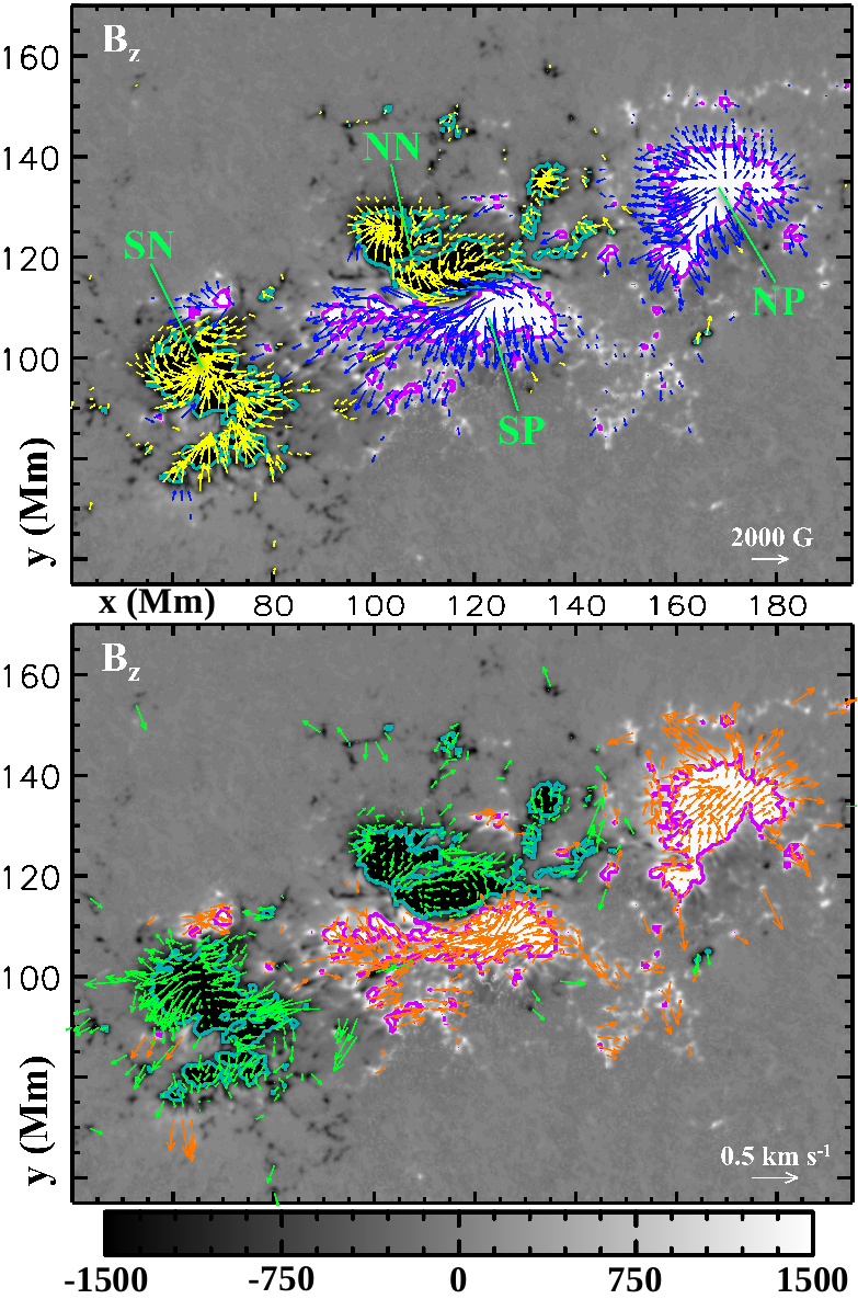
Figure 1.— Top: SDO/HMI photospheric vector-magnetogram at $\sim$ 06:28 UT. The gray scale displays the vertical component, $B_{z}$ (in Gauss), while the yellow/blue arrows show the transverse component of the magnetic field. Bottom: vertical magnetic field overplotted with the flux transport velocity field (green/orange arrows). Pink and cyan solid lines show $B_{z}=\pm 500\ \mathrm{Gauss}$ isocontours.

We test the robustness of the connectivity-based helicity flux density method against different magnetic field extrapolation models of the internally complex AR 11158. This AR appeared on the solar disk at the heliographic coordinates S19 E42 on 2011 February 10. The AR was the result of fast and strong magnetic flux emergence that produced two large-scale bipoles, a northern and a southern one, in close proximity (see LABEL:Fig-BFTV; e.g., Schrijver et al., 2011). The complex, quadrupolar magnetic field of this AR produced several C-/M-/X-class flares and CMEs during its on-disk passage (e.g., Toriumi et al., 2014). A large fraction of this flaring activity was associated with the collision between the negative magnetic polarity of the northern bipole, NN, and the positive magnetic polarity of the southern bipole, SP, which led to a strong and continuous shearing of their polarity inversion line. More details on the configuration, evolution, and flaring activity of the AR can be found in e.g., Sun et al. (2012), Jiang et al. (2012), Vemareddy et al. (2012a) and Inoue et al. (2013).

The coronal models of AR 11158 are computed using vector magnetograms taken by the Helioseismic and Magnetic Imager (HMI, e.g., Schou et al., 2012) onboard the Solar Dynamics Observatory (SDO, e.g., Pesnell et al., 2012). SDO/HMI provides full-disk vector magnetograms of the Sun with a pixel size of 0.5^′′. For the purpose of this paper, we re-use part of the data from Dalmasse et al. (2013) who had applied the connectivity-based approach to AR 11158 with an NLFFF extrapolation without addressing the possible dependency of the results on the choice of extrapolation method. In particular, vector magnetograms at 06:22 UT and 06:34 UT on 2011 February 14 from the HMI-SHARP data series, HARP number 377 (Hoeksema et al., 2014) are re-used.

These two vector magnetograms are used to derive the photospheric flux transport velocity field with the differential affine velocity estimator for vector magnetograms (DAVE4VM; Schuck, 2008), using a window size of 19 pixels as suggested by Liu et al. (2013). The computed flux transport velocity field effectively represents an instantaneous flux transport velocity field at $\sim$ 06:28 UT. The two vector magnetograms taken at 06:22 UT and 06:34 UT are averaged to construct an instantaneous vector magnetogram associated with the flux transport velocity field at $\sim$ 06:28 UT. The constructed vector magnetic field is then used both to compute $G_{\theta}$ and as the photospheric boundary condition for the different FFF extrapolations presented Section 4. The vector magnetic field and flux transport velocity field at $\sim$ 06:28 UT are shown in LABEL:Fig-BFTV.

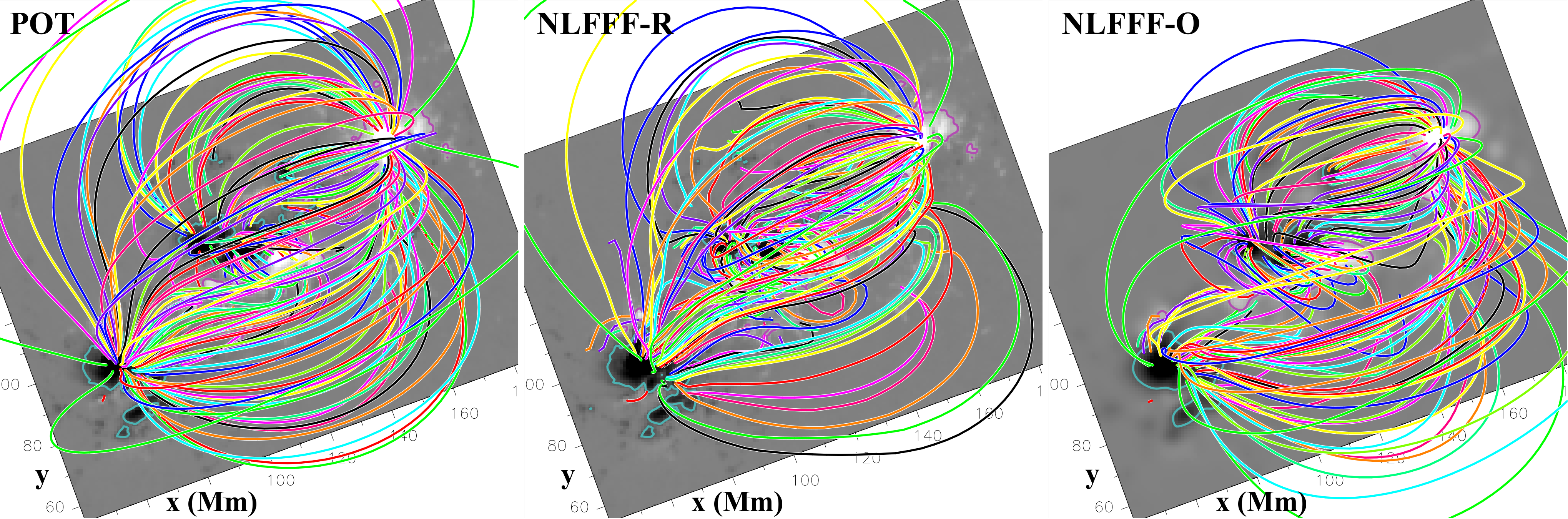
Figure 2.— Selected closed field lines of the 3D extrapolated magnetic field for the potential field (labelled POT; left), the NLFFF from the magneto-frictional relaxation method (labelled NLFFF-R; middle), and the NLFFF from the optimization method (labelled NLFFF-O; right). The magnetic field lines were integrated from the same -randomly selected- photospheric footpoints for all three extrapolations (the same colour is used for the same footpoint). The gray scale displays the photospheric vertical magnetic field, $B_{z}$, with $\pm 500$ Gauss isocontours (purple and cyan solid lines).

3.2. Estimation of Helicity-Flux Uncertainties

As part of testing the reliability of the connectivity-based helicity flux density method, we also wish to evaluate uncertainties in $G_{\theta}$ and $G_{\Phi}$ maps caused by those in the photospheric magnetic field. In particular, our error analysis includes both the effect of photon noise ($\approx 10$ Gauss) and several sources of systematic errors. Hoeksema et al. (2014) recently performed an extensive analysis of the uncertainties in the measurements of the magnetic field strength by SDO/HMI. In particular, they focused on the uncertainty analysis for NOAA 11158. Among several sources of systematic errors, including those related with the inversion code, they found that the dominant contribution of uncertainty in SDO/HMI magnetic field measurements is coming from the daily variation of the radial velocity of the spacecraft along its geosynchronous orbit. Their analysis concludes that the typical uncertainty in SDO/HMI measurements of the magnetic field strength is about 100 Gauss. The latter can be easily checked from the estimated field-strength error map of NOAA 11158 provided by the SDO/HMI pipeline and which can be downloaded from JSOC. We also want to compare these errors with those related with the choice of magnetic field extrapolation used to compute $G_{\Phi}$.

For that purpose, we conduct a Monte Carlo experiment as proposed by Liu & Schuck (2012) for error estimation of the total helicity flux. Random noise with a Gaussian distribution having a width ($\sigma$) of 100 Gauss is added to all three components of the magnetic field for both vector magnetograms taken at 06:22 UT and 06:34 UT. 100 Gauss is the $\approx 1\sigma$ uncertainty in the total magnetic field strength from HMI data estimated by Hoeksema et al. (2014) and further reported in Bobra et al. (2014). The uncertainty is then propagated through the chain of helicity flux density calculations to the flux transport velocity field at the photosphere derived from DAVE4VM, the corresponding vector magnetogram at $\sim$ 06:28 UT, and finally to the $G_{\theta}$ and $G_{\Phi}$ maps.

Although they did not perform a full parametric analysis, Wiegelmann et al. (2006) showed that extrapolations with the optimization method were not significantly affected by modest noise in the photospheric vector magnetogram. They found that the preprocessing of the photospheric data towards a more force-free state (see e.g., Section 4.2) strongly helps in that matter. This may be expected considering that the random noise on the photospheric vector magnetic field acts as a source of non-force-free signals on high spatial frequencies while the preprocessing filters such signals out. Even if FFF reconstructions would likely be differently affected by noise in the photospheric data, its global effect on the extrapolations should be limited by the preprocessing stage. On the other hand, FFF extrapolations are more likely to be affected by more global effects including, but not limited to, large-scale non-force-free regions not suppressed by the preprocessing, magnetic flux imbalance, and lateral boundary conditions. Then, as far as $G_{\Phi}$ is concerned, the effect of random noise on the extrapolation results is to introduce uncertainties in the connectivity of the magnetic field. In this regard, we believe that the choice of extrapolation method and preprocessing level is more fundamental and has a stronger impact on the magnetic connectivity, and hence, on $G_{\Phi}$. For these reasons, we decided not to propagate the noise to the FFF extrapolations.

The noise propagation experiment is repeated 100 times, producing 100 noise-added $G_{\theta}$ and $G_{\Phi}$ maps for all three FFF extrapolations considered in this paper. For each scalar quantity, $\mathcal{F}$, the $1\sigma$ estimated error, $\sigma_{\mathcal{F}}$, is computed as the mean, over all the $n$ pixels of the map, of the root mean square of the $N=100$ noise-added $\mathcal{F}$-maps, $\mathcal{F}_{\mathrm{n.a.}}^{i}\left({\mathbf{x}}_{j}\right)$, compared with the no-noise $\mathcal{F}$-map, $\mathcal{F}_{\mathrm{n.n.}}\left({\mathbf{x}}_{j}\right)$

$$\sigma_{\mathcal{F}}=\frac{1}{n}\sum^{n}_{j=1}\left(\frac{1}{N}\sum^{N}_{i=1}\left(\mathcal{F}_{\mathrm{n.a.}}^{i}\left({\mathbf{x}}_{j}\right)-\mathcal{F}_{\mathrm{n.n.}}\left({\mathbf{x}}_{j}\right)\right)^{2}\right)^{\frac{1}{2}}\,.$$ (14)

4. Force-Free Magnetic Field Extrapolations

We perform three force-free field extrapolations using different assumptions and methods: (1) the potential magnetic field, (2) a nonlinear FFF (NLFFF) reconstruction using the magneto-frictional method of Valori et al. (2010), and (3) an NLFFF generated with the optimization method of Wiegelmann (2004). The extrapolations and setup used to produce them are described hereafter.

At this stage, we wish to emphasize that many more extrapolation assumptions, methods, and implementations, exist in the literature. These different methods are further distinguished in terms of the physical information that they extract from the photospheric vector magnetograms and use as boundary conditions. For instance, some NLFFF codes use vector magnetograms as boundary conditions, as is the case of the magneto-frictional relaxation implemented by, e.g., Valori et al. (2010), or the optimization method implemented by, e.g., Wiegelmann & Inhester (2010). Others built on the Grad-Rubin approach (Grad & Rubin, 1958) use the normal component of the photospheric magnetic field and the force-free parameter – derived from the vector magnetograms – as boundary conditions (e.g., Amari et al., 2006; Wheatland, 2007). Recently, Malanushenko et al. (2012) also proposed a Quasi-Grad-Rubin method that only uses the photospheric normal magnetic field, but combined with coronal loops fitting to constrain the coronal distribution of the force-free parameter. Finally, several codes haven been recently developed to perform a full MHD relaxation using photospheric vector magnetograms, thus distinguishing them from NLFFF models through the inclusion of plasma forces in the reconstruction of the 3D magnetic field of ARs (e.g., Inoue & Morikawa, 2011; Jiang & Feng, 2012; Zhu et al., 2013). All these different codes and methods can be used to model the coronal magnetic field of ARs from which we can derive the magnetic connectivity required to use the connectivity-based helicity flux density approach to map the helicity flux in ARs.

Several of these methods have been compared with each others in e.g., DeRosa et al. (2009, 2015), including the two NLFFF methods used in this paper. From these studies, it appears that the three extrapolation methods considered here generally produce differences in field-lines distribution that are representative of the differences that can be expected between the coronal magnetic fields reconstructed with other FFF methods. We thus expect the differences in the $\mathrm{d}h_{\Phi}/\mathrm{d}t$ and $G_{\Phi}$ calculations presented in this paper to be representative of the differences that would be obtained when computing the connectivity-based helicity flux density with other extrapolation methods. For this reason, we limit ourselves to the analysis of helicity flux density calculations with the three extrapolations described below.

The extrapolation presented hereafter are performed on a finite field of view with open side and top boundaries, but without assuming magnetic flux balance. Magnetic flux is thus free to leave the extrapolation domain as open-like magnetic field. Such open-like magnetic field may represent truly open magnetic field and/or connections with the very distant quiet Sun and surrounding ARs. Helicity flux density calculations are not performed for open-like field lines because $G_{\Phi}$ and $\mathrm{d}h_{\Phi}/\mathrm{d}t$ are not defined for open magnetic flux tubes (cf. Section 2.2). For that reason, open field lines are not plotted in any of the field-line plots presented throughout the paper.

Working with a finite field of view may be a strong limitation to reconstruct the magnetic field of ARs. Not only is the entire photosphere always populated with quiet Sun magnetic flux, but there are also often more than one AR on the Sun at a given time (e.g., Schrijver et al., 2013). The effect of using a limited field of view is to remove large-scale connections with the distant quiet Sun and surrounding ARs that are outside the field of view considered for the extrapolation. Such distant connections may influence the results of the helicity flux density calculations with the connectivity-based method. To test such an influence, one needs to compare the connectivity-based helicity flux density computed from a global, full-Sun magnetic field reconstruction in spherical geometry vs. from a local magnetic field extrapolation. However, current global reconstructions of the solar magnetic field are limited by the fact that there is no full-Sun vector magnetograms at any single time, and hence, no proper data for the boundary conditions of full-Sun extrapolation codes. A proper analysis of the effect of distant ARs on the helicity flux density calculations would therefore require numerical modeling. Such a study is not the goal of the present work. The vast majority of investigations relying on NLFFF extrapolations are focusing on single ARs with the same type of limited field of view and inherent hypotheses that are also used in the present manuscript. We are presently testing the reliability of connectivity-based helicity flux density calculations with regard to such NLFFF modeling, i.e., we aim to determine if and to which extent different choices of NLFFF computation schemes applied to a compact active region can impact the distribution of the helicity flux density.

4.1. Potential Field

The current-free magnetic field is the minimal-energy possible state for the given distribution of magnetic field at the boundaries of the considered volume. In addition, the potential field is often used as an initial state of numerical methods that build the more complex NLFFF models (see review by, e.g., Wiegelmann & Sakurai, 2012). It is therefore an important candidate to consider for testing the connectivity-based helicity flux density method, despite its limitation in reproducing nonlinear features of the coronal field.

The potential field can be directly computed using the potential theory and the reflection principle to solve the Laplace equation for the scalar potential in terms of the flux through the photospheric boundary (Schmidt, 1964). However, in order to speed up the calculation, such a method is actually used only to compute the scalar potential on all six boundaries of the considered volume. The magnetic scalar potential in the volume is then computed solving the Laplace equation, subjected to the obtained Dirichlet boundary conditions, using a fast Helmholtz solver from the Intel Mathematical Kernel Library. For the required vertical component of the field on the lower boundary, the same vertical component as for the NLFFF extrapolation described Section 4.2 is used. The potential field extrapolation is referred to as POT in the following and selected field lines for this extrapolation are shown in the leftmost panel of LABEL:Fig-B3D.

4.2. NLFFF from Magneto-Frictional Relaxation

NLFFF extrapolations are models of the coronal magnetic field that assume the corona to be static on the time scale of interest, and to be dominated by magnetic forces that are distributed in a way such that the resulting Lorentz force is everywhere vanishing. Such assumptions are supposed to be valid in the entire volume of interest, boundaries included. The magneto-frictional relaxation method implements numerical relaxation and multi-grid techniques to solve the corresponding equations (see Valori et al., 2007, 2010; DeRosa et al., 2015, for more details).

The remapped and disambiguated vector magnetograms from the HMI-SHARP data series were interpolated to 1^′′-resolution and averaged to construct the vector magnetogram at 06:28 UT (cf. Section 3.1) used for the NLFFF extrapolation. Vector magnetograms are inferred from spectropolarimetric measurements taken at photospheric heights, where the plasma is non-force-free. Therefore, in order to use the vector magnetogram as a boundary condition for the NLFFF extrapolation code, the forces acting on the magnetogram need to be reduced (preprocessing). To this purpose we use the method of Fuhrmann et al. (2007, 2011). In this application, only the horizontal components of the field are preprocessed, yielding a reduction of the forces from 0.035 to 0.002 in the non-dimensional units used in Metcalf et al. (2008). Since smoothing is not necessarily facilitating the extrapolation (Valori et al., 2013), no smoothing was applied. The resulting magnetogram was then extrapolated using the magneto-frictional code into a volume of about $208\times 202\times 145$ Mm³.

The resulting extrapolated field has solenoidal errors that can be quantified using the formula by Valori et al. (2013) into $9\%$ of the total magnetic energy. The fraction of the total current that is perpendicular to the field is $\sigma_{J}=0.48$ (Wheatland et al., 2000), a rather high value that is not uncommon for extrapolation of HMI vector magnetograms with the magneto-frictional method (see Valori et al., 2012, for an application to Hinode/SP magnetogram with a much lower $\sigma_{J}$). Selected field lines of the NLFFF obtained in this way, and referred to as NLFFF-R in the following, are shown in the central panel of LABEL:Fig-B3D.

Figure 3.— Surface densities of helicity flux for AR 11158 at $\sim$ 06:28 UT on 2011/02/14 (in units of $10^{7}$ Wb² m^-2 s^-1) computed from the purely photospheric proxy ($G_{\theta}$; top left) and the connectivity-based proxy ($G_{\Phi}$) derived using the three FFF extrapolations (top right, and bottom row). Purple and cyan solid lines show $B_{z}=\pm 500\ \mathrm{Gauss}$ isocontours from the original photospheric vector magnetogram of SDO/HMI. The presence of strong white (i.e., zero) signals in the left part of SN and north-right part of NP for all three $G_{\Phi}$ maps is due to open-like magnetic flux where $\mathrm{d}h_{\Phi}/\mathrm{d}t$ and $G_{\Phi}$ are not defined, and hence, not computed.

4.3. NLFFF from Optimization Method

For the second NLFFF model considered in this paper, we use the weighted optimization method (Wiegelmann, 2004), which is an implementation and modification of the original optimization algorithm of Wheatland et al. (2000). The optimization method minimizes an integrated joint measure, which comprises the normalized Lorentz force, the magnetic field divergence, and treatment of the measurement errors, over the computational domain (see Wiegelmann & Inhester, 2010; Wiegelmann et al., 2012, for more details).

To perform the extrapolation, the vector magnetogram (LABEL:Fig-BFTV) is first rebinned to 1^′′ per pixel and preprocessed towards the force-free condition using the method of Wiegelmann et al. (2006). The extrapolation is finally performed on a uniform grid of $256\times 256\times 200$ points covering $\sim 185\times 185\times 144$ Mm³. We find a solenoidal error of $1\%$ of the total magnetic energy and a fraction of total current perpendicular to the magnetic field $\sigma_{J}=0.20$. These values are lower than for the NLFFF-R model (Section 4.2), which is due both to different preprocessing and extrapolation methods and strategies.

In the following, the NLFFF model built with the optimization method is referred to as NLFFF-O. A set of selected magnetic field lines is shown in the rightmost panel of LABEL:Fig-B3D.

5. Results

In this section, we analyze the results from the connectivity-based helicity flux density calculations. The validation of the maps, error estimations, and qualitative comparisons are briefly presented in Section 5.1. The one-to-one quantitive comparisons are discussed in Section 5.2.

5.1. Helicity-Flux Density Distribution

Table 1Metrics for validation and quantification of $G_{\Phi}$ maps

FFF model	$\tau_{\Phi_{\mathrm{imb.}}}$	$C_{{\mathcal{S}}_{\Phi_{\mathrm{cl.}}}}$	$C_{+}$	$C_{-}$
POT	+$1.2\times 10^{-3}$	$4.2\times 10^{-4}$	1.32	1.71
NLFFF-R	$-7.6\times 10^{-3}$	$4.7\times 10^{-2}$	1.21	1.67
NLFFF-O	+$2.6\times 10^{-3}$	$3.2\times 10^{-2}$	1.23	1.57

Note. — The table presents the validation and quantification metrics for the maps displayed in LABEL:Fig-surface-densities. All metrics are dimensionless ratios defined by Equations (10) – (13).

Table 1 presents the validation metrics for the $G_{\Phi}$ maps computed from the three FFF extrapolation models described Section 4. For all three $G_{\Phi}$ maps, we obtain $\tau_{\Phi_{\mathrm{imb.}}}$ below $1\%$ and $C_{{\mathcal{S}}_{\Phi_{\mathrm{cl.}}}}$ below $5\%$. This allows us to verify that the magnetic flux over which the connectivity-based helicity flux density is computed is very well balanced and that the calculation of $\mathrm{d}h_{\Phi}/\mathrm{d}t$ and $G_{\Phi}$ well preserves the total helicity flux in that region in the closed magnetic flux. Together, these numbers enable us to confirm the accuracy of the $G_{\Phi}$ and $\mathrm{d}h_{\Phi}/\mathrm{d}t$ calculations discussed in the following.

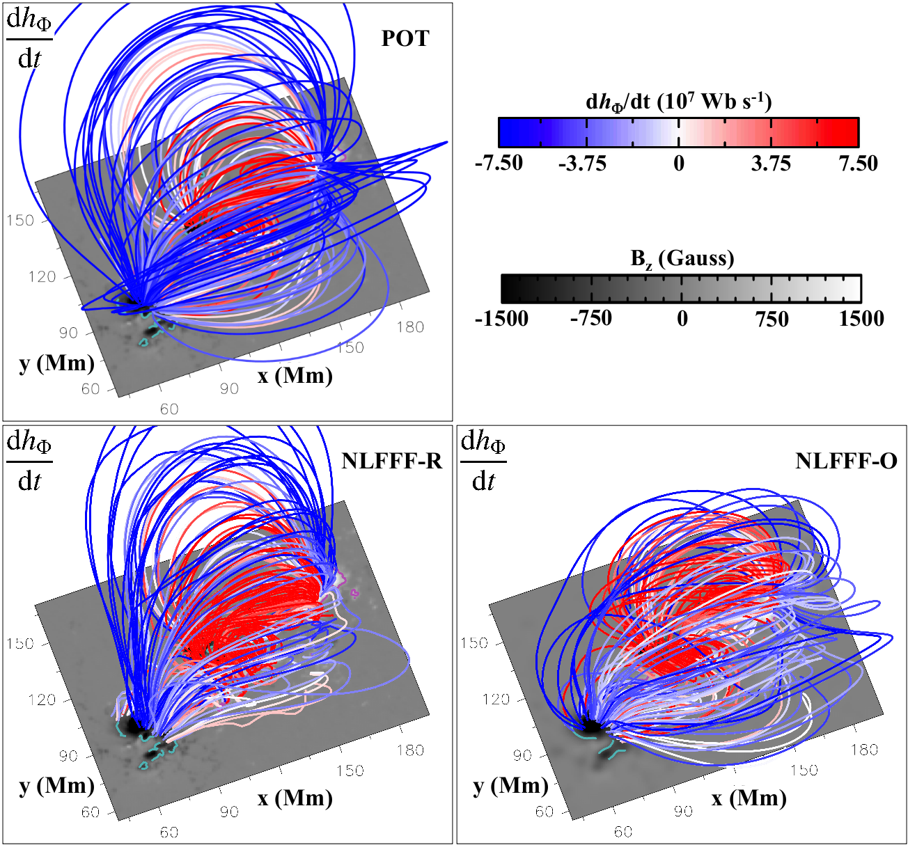
Figure 4.— 3D representation of the connectivity-based helicity flux density for each FFF extrapolation. The magnetic field lines were integrated from the same -randomly selected- photospheric footpoints for all three extrapolations. They are colored according to their $\mathrm{d}h_{\Phi}/\mathrm{d}t$ value. Purple and cyan solid lines show $B_{z}=\pm 500\ \mathrm{Gauss}$ isocontours from the FFF extrapolation.

LABEL:Fig-surface-densities presents the surface density of helicity flux from the purely photospheric proxy, $G_{\theta}$, and the connectivity-based proxy, $G_{\Phi}$, computed from all three FFF extrapolations. The mean of the absolute value of the helicity flux signal in most of the AR (i.e., $|B_{z}|\geq 100$ G) is $2.8\times 10^{6}$ Wb² m^-2 s^-1 for the $G_{\theta}$ map and $1.7\times 10^{6}$ Wb² m^-2 s^-1 for the $G_{\Phi}$ maps, while a large fraction of the maps is associated with local helicity fluxes of $10^{7}$ Wb² m^-2 s^-1. As shown in Table 2, the errors for $G_{\theta}$ and $G_{\Phi}$ estimated from our Monte Carlo experiment are $3.7\times 10^{5}$ Wb² m^-2 s^-1 for $G_{\theta}$ and lower than $3\times 10^{5}$ Wb² m^-2 s^-1 for $G_{\Phi}$. The signal intensity of the surface density maps in LABEL:Fig-surface-densities is thus well above the estimated noise level.

Table 2Error estimations from Monte Carlo experiment

	$G_{\theta}$	$G_{\Phi}($POT$)$	$G_{\Phi}($NLFFF-R$)$	$G_{\Phi}($NLFFF-O$)$
$\sigma$	3.7	2.6	2.2	3.0

Note. — The errors are in units of $10^{5}$ Wb² m^-2 s^-1, i.e., $\sim 10-100$ times smaller than the typical values displayed by the $G_{\theta}$ and $G_{\Phi}$ maps from LABEL:Fig-surface-densities. See Section 3.2 for a description of error calculations.

LABEL:Fig-surface-densities shows that the largest differences in helicity flux density maps are between $G_{\theta}$ and the three $G_{\Phi}$ maps. In particular, the strongest differences are associated with magnetic flux systems that connect footpoints of opposite $G_{\theta}$ signs, i.e., footpoints of NN connected to NP, footpoints of SN connected to SP, and footpoints of SN connected to NP. On the other hand, the $G_{\theta}$ map is relatively similar to the three $G_{\Phi}$ maps for the flux system connecting NN to SP, because magnetic field lines are connecting footpoints with similar values of $G_{\theta}({\mathbf{x}})/|B_{n}({\mathbf{x}})|$. This is consistent with the work of Pariat et al. (2005) and Dalmasse et al. (2014) who showed that $G_{\theta}$ hides the true helicity flux signal when simultaneous opposite helicity fluxes are present in a magnetic configuration. This effect is inherent to the definition of $G_{\theta}$ that does not acknowledge the fact that the variation of magnetic helicity in an elementary magnetic flux tube comes from the motions of its two photospheric footpoints with respect to the other elementary flux tubes of the entire magnetic configuration. As a result, the comparison of the total positive helicity flux and total negative helicity flux from $G_{\theta}$ in the closed magnetic flux with the same quantities computed for each one of the $G_{\Phi}$ maps leads values of $C_{+}>1.2$ and $C_{-}>1.5$ (see Table 1). Such values indicate that $G_{\theta}$ is affected by moderate spurious positive signals and rather high spurious negative helicity fluxes that are corrected for by the use of $G_{\Phi}$ (cf. Section 2.3). LABEL:Fig-surface-densities thus highlights the fact that the redistribution of helicity flux operated by $G_{\Phi}$ is crucial to the photospheric mapping of helicity flux in ARs, regardless of the coronal magnetic field modeling.

All three $G_{\Phi}$ maps in LABEL:Fig-surface-densities are in very good qualitative agreement, showing (i) a negative helicity flux in SN, (ii) a strong positive helicity flux in NN and SP, and (iii) strong positive and negative helicity fluxes with a strongly marked interface in NP. The $G_{\Phi}$ maps from the two NLFFF models are very similar. Setting aside the white signal in SN, which is due to open field-lines where $G_{\Phi}$ is not computed, and focusing on the common areas where all three extrapolations have closed magnetic flux, we find that the helicity flux density map derived from the potential field is also similar to the $G_{\Phi}$ maps derived from the two NLFFF models. The most noticeable difference is in the south-east part of NN that does not show any significant helicity flux for $G_{\Phi}($POT$)$, contrary to both $G_{\Phi}($NLFFF-R$)$ and $G_{\Phi}($NLFFF-O$)$.

Finally, the good qualitative agreement between the connectivity-based helicity flux density calculations from the three FFF extrapolations is further emphasized by the 3D representation of $\mathrm{d}h_{\Phi}/\mathrm{d}t$ in LABEL:Fig-dhphi. They all show that the inner part of the AR is dominated by strong positive helicity fluxes and is embedded within a magnetic field region dominated by strong negative helicity fluxes. The core results of Dalmasse et al. (2013) are thus confirmed with a weak dependance on the extrapolation method.

5.2. Quantitative Analysis

We now focus on the quantitative comparison of the helicity flux density calculations obtained from the three FFF models. We restrict our analysis to the pixels of the $G_{\Phi}$ maps that are above the noise level (different for each map) estimated from the Monte Carlo experiment. The error levels are given in Table 2.

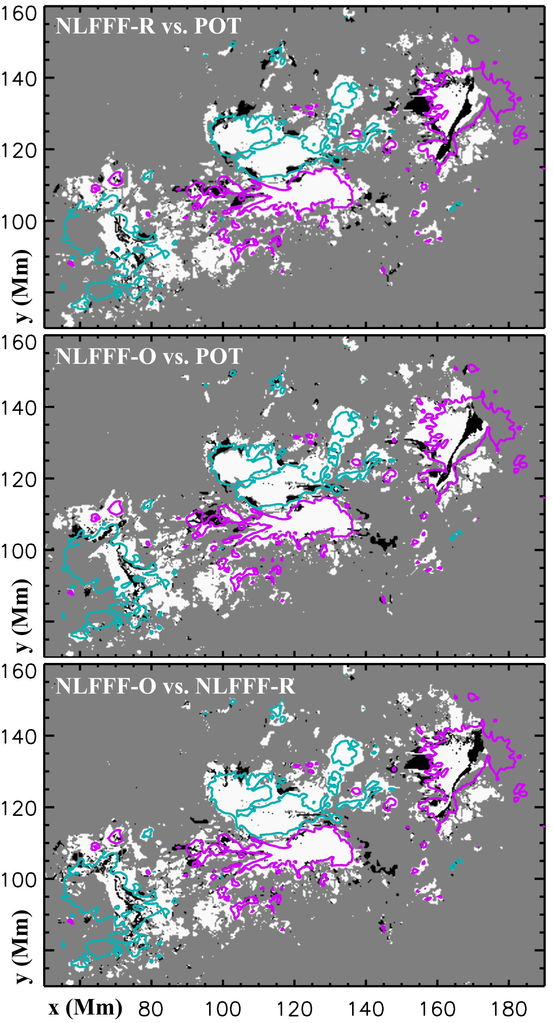
Figure 5.— Maps of $G_{\Phi}$-sign agreement between the surface-density maps obtained with the three FFF models. For each map, $[$white; black$]=[$agree; disagree$]$, while gray corresponds to pixels that are either associated with open-like field-lines (where $G_{\Phi}$ is not computed) or where $G_{\Phi}$ is below the noise level for at least one of the two models being compared. Purple and cyan solid lines show $B_{z}=\pm 500\ \mathrm{Gauss}$ isocontours from the original photospheric magnetogram of SDO/HMI.

LABEL:Fig-Sign-Agreement displays the three maps of sign agreement. The regions where our analysis can be carried out (white and black) is mostly associated with the strong magnetic field of AR 11158, i.e., where $|B_{z}|\gtrsim 500$ Gauss. These regions correspond to the area where most of the helicity flux (at least $88\%$ of the total unsigned helicity flux) computed with $G_{\Phi}$ is coming from. This is because the helicity flux intensity outside these regions is below the noise level of the respective $G_{\Phi}$ maps. Despite the presence of some relatively small areas of disagreement (black patches), we find that these regions are dominated by agreement (white signal) over the sign of helicity flux derived using different FFF extrapolations. In particular, the percentage of surface area for which pairs of $G_{\Phi}$ maps agree is always larger than $85\%$, which translates into more than $\approx 84\%$ in terms of magnetic flux. Therefore, the local sign of helicity flux computed from the connectivity-based helicity flux density method is very robust to the different FFF models and assumptions used for calculations.

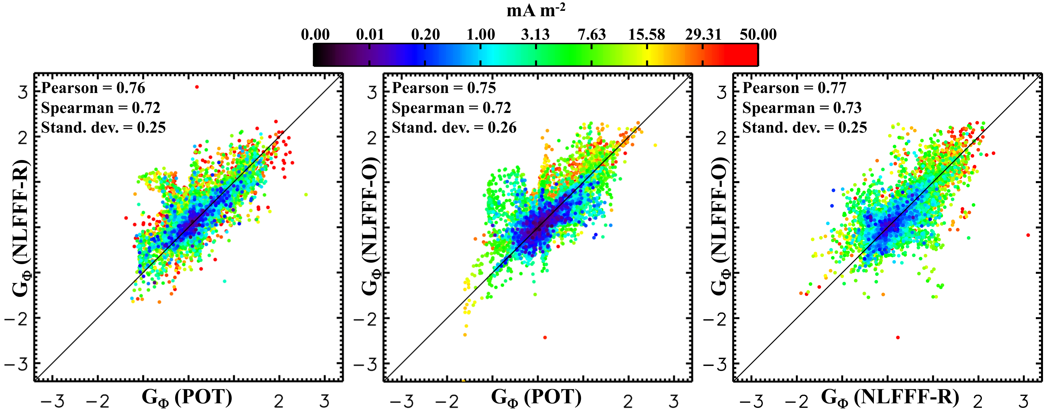
Figure 6.— Scatter plots of pixel-to-pixel comparison of the surface-density of helicity flux. The black solid line shows the $y=x$ line. “Pearson”, “Spearman”, and “Stand. dev.” respectively are the Pearson correlation coefficient, the Spearman correlation coefficient, and the standard deviation. The standard deviation is in units of $10^{7}$ Wb² m^-2 s^-1. From the left to the right panel, the color scale corresponds to $|j_{z}($NLFFF-R$)|$, $|j_{z}($NLFFF-O$)|$, and $\sqrt{|j_{z}(\textrm{NLFFF-R})|\cdot|j_{z}(\textrm{NLFFF-O})|}$. Notice the color scale for the current density is not linear, but was instead chosen as $\|\cdot\|^{1/4}$ with saturation at $50$ mA m^-2 for dynamic range optimization.

LABEL:Fig-Scatter displays the linear correlation plots of $G_{\Phi}$ values in each pixel, for different pairs of FFF extrapolations. For comparisons between $G_{\Phi}$ from the potential field model and one of the two NLFFFs, the points are colored according to the strength of the photospheric electric current density, $|j_{z}|$, from the different preprocessed boundary employed in the NLFFF model under consideration. For the plot comparing $G_{\Phi}$ from the two NLFFF extrapolations, the points are colored according to $(|j_{z}($NLFFF-R$)|\cdot|j_{z}($NLFFF-O$)|)^{1/2}$. Such a color coding was introduced in order to investigate the dependency of the scatter on the electric current density of magnetic field lines where $G_{\Phi}$ is computed.

In each scatter plot, we find that the spatial distribution of points exhibits a clear ellipsoidal shape aligned along the $y=x$ diagonal line. Each one of these distributions display a moderate dispersion. The three standard deviations computed from each scatter plot of LABEL:Fig-Scatter are $\leq 2.6\times 10^{6}$ Wb² m^-2 s^-1, which is 5 to 10 times smaller than most of the signal in the four main magnetic polarities. These standard deviations are $\approx 10$ times larger than the $G_{\Phi}$ errors estimated from the Monte Carlo experiment (Table 2). As anticipated, it means that, despite the substantial agreement on the sign of the injected helicity between different extrapolations, a significant uncertainty in the connectivity-based calculations is coming from the choice of extrapolation model used to derive the field line connectivity.

Table 3Scatter plots dispersion vs. electric current density

$j_{z}$	$]0,0.2]$	$]0.2,3.1]$	$]3.1,15.6]$	$]15.6,50.0]$
+$\sigma_{G_{\Phi}}$	$[1.5,1.8]$	$[1.8,2.0]$	$[2.6,3.6]$	$[3.0,4.1]$

Note. — The interval for the standard deviation, $\sigma_{G_{\Phi}}$, is derived from the values obtained for the three scatter plots of LABEL:Fig-Scatter. The electric current density is in units of mA m^-2 and the dispersion in units of $10^{6}$ Wb² m^-2 s^-1. From left to right, the five ranges of electric current density correspond to $]\mathrm{black};\ \mathrm{dark\ blue}]$, $]\mathrm{dark\ blue};\ \mathrm{green}]$, $]\mathrm{green};\ \mathrm{yellow}]$, and $]\mathrm{yellow};\ \mathrm{red}]$ of the color-scale in LABEL:Fig-Scatter.

LABEL:Fig-Scatter further shows that the ellipsoidal pattern of the distribution of points is present independently of the electric current density, i.e., of the color of the points. We also notice that the scattering of points away from the $y=x$ line presents some relatively weak dependance on the electric current density of the field lines used for the connectivity-based calculations. In particular, we find a dispersion in the range $\approx[1.5,2.0]\times 10^{6}$ Wb² m^-2 s^-1 for black to green points, and $\approx[2.6,4.1]\times 10^{6}$ Wb² m^-2 s^-1 for green to red points (finer details are provided in Table 3). In addition, the number of pixels with average-to-strong electric current density (i.e., green to red points) is sensibly the same as the number of pixels with very weak-to-average electric current density (i.e., black to green points). This implies that the correlation coefficients, displayed in LABEL:Fig-Scatter and discussed below, are not dominated by the differences in $G_{\Phi}$ values from nearly-potential magnetic field lines.

For all three scatter plots, we find that the Pearson, $c_{P}$, and Spearman, $c_{S}$, correlation coefficients are such that $c_{P}\geq 0.75$ and $c_{S}\geq 0.72$. We checked that these values are statistically significant by conducting a null hypothesis test (details and results of this test are provided in Appendix A). We therefore conclude that the calculations of the connectivity-based helicity flux density derived from different FFF extrapolations are highly correlated and consistent with each other.

For further comparison, we compute the vector correlation metric, $C_{\mathrm{vec}}$, comparing the three 3D magnetic field extrapolations as defined by Equation (28) of Schrijver et al. (2006). For that purpose, the POT and NLFFF-R 3D magnetic fields are interpolated on the same grid as the NLFFF-O (whose extrapolation domain is common to all three models) using trilinear interpolation. We find $C_{\mathrm{vec}}({\mathbf{B}}_{\mathrm{NLFFF-R}},{\mathbf{B}}_{\mathrm{POT}})=0.84$, $C_{\mathrm{vec}}({\mathbf{B}}_{\mathrm{NLFFF-O}},{\mathbf{B}}_{\mathrm{POT}})=0.90$, and $C_{\mathrm{vec}}({\mathbf{B}}_{\mathrm{NLFFF-O}},{\mathbf{B}}_{\mathrm{NLFFF-R}})=0.90$. Such values for the vector correlation metric of the magnetic fields are very high even though the 3D distributions of the magnetic field lines are relatively different when comparing the three extrapolations, as inferred from LABEL:Fig-B3D. We thus find that the vector correlation metric for the magnetic fields is higher than the Pearson and Spearman correlation coefficients found when comparing the helicity flux density calculations.

6. Discussion

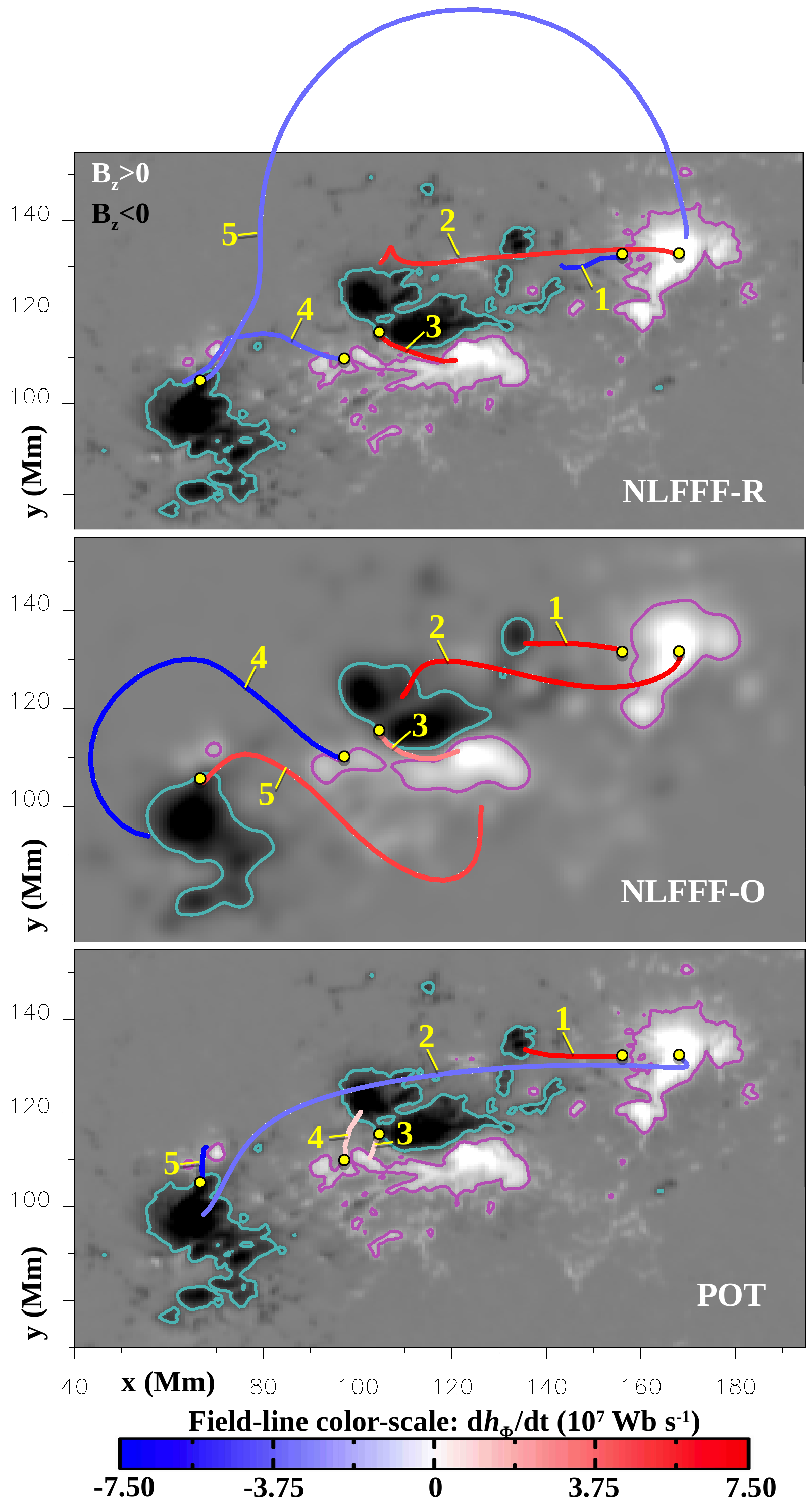
Figure 7.— 3D representation (top view) of the connectivity-based helicity flux density, as in LABEL:Fig-dhphi, illustrating local differences between $\mathrm{d}h_{\Phi}/\mathrm{d}t$ from the different FFF extrapolations. The magnetic field lines are labelled according to the common photospheric footpoint from which they were integrated and which is indicated by the yellow disk. The color scale for the vertical magnetic field (gray scale) and its isocontours are the same as in LABEL:Fig-dhphi.

At this point, we wish to emphasize that the robustness of the connectivity-based method against different magnetic field extrapolations does not mean that the extrapolations are very much alike. On the contrary, all three extrapolations considered here produce 3D magnetic fields that are different from each other as shown in LABEL:Fig-B3D. So, what does it mean that the connectivity-based helicity flux density calculations are robust against different extrapolation methods?

First of all, we remind the reader that the surface-density of helicity flux, $G_{\Phi}$, only explicitly depends on the connectivity of magnetic field lines and not on their 3D geometry; the latter only has an implicit effect on $G_{\Phi}$ by affecting the magnetic connectivity. Secondly, expanding Equation (9) using Equation (7) leads to

$$G_{\Phi}({\mathbf{x}}_{+})=\frac{|B_{n}({\mathbf{x}}_{+})|}{2}\left(\dot{\Theta}_{B}({\mathbf{x}}_{+})-\dot{\Theta}_{B}({\mathbf{x}}_{-})\right)\,.$$ (15)

Equation (15) shows that, for a given footpoint ${\mathbf{x}}_{+}$, the helicity flux density $G_{\Phi}$ from different extrapolation models will be exactly the same (1) if they have the exact same magnetic field connectivity, or (2) if they have a different connectivity, the first extrapolation links ${\mathbf{x}}_{+}$ to ${\mathbf{x}}_{1_{-}}$ and the second links ${\mathbf{x}}_{+}$ to ${\mathbf{x}}_{2_{-}}\neq{\mathbf{x}}_{1_{-}}$, but $\dot{\Theta}_{B}({\mathbf{x}}_{2_{-}})=\dot{\Theta}_{B}({\mathbf{x}}_{1_{-}})$. The same type of conclusion can be drawn for $G_{\Phi}({\mathbf{x}}_{-})$ by simply exchanging ${\mathbf{x}}_{+}$ and ${\mathbf{x}}_{-}$. Note that condition (2) relates to the spatial smoothness of $\dot{\Theta}_{B}({\mathbf{x}})$ and, by extension, $G_{\theta}({\mathbf{x}})$.

In general, $G_{\Phi}$ can distinguish two magnetic fields that have different photospheric magnetic connectivities. This is evident from the connectivity-based flux density maps shown LABEL:Fig-surface-densities and the clear dispersion shown in the scatter plots of LABEL:Fig-Scatter. However, we argue that as long as two different 3D magnetic fields have, on average, a similar magnetic connectivity, then the $G_{\Phi}$ maps computed from these magnetic fields should display a good overall agreement. Note that, although not discussed, this was already observed by Dalmasse et al. (2014) for the models analyzed in their Figures 8, 10, 11, and 12. The strongest differences would then be expected in localized regions where the magnetic connectivity from the extrapolations is markedly different, typically in the close surroundings of quasi-separatrix layers (QSLs) which are regions of strong gradients of the magnetic connectivity that are favorable to magnetic reconnection (e.g., Démoulin et al., 1996; Titov et al., 2002; Aulanier et al., 2006; Janvier et al., 2013). This is indeed what we find in our analysis of AR 11158, e.g., at the interface of positive and negative helicity fluxes in NP (see LABEL:Fig-surface-densities) that coincides with a large-scale QSL that separates field-lines connecting NP to NN and NP to SN.

Then, we recall that $G_{\Phi}$ is only a 2D representation of the physical, 3D, definition of local magnetic helicity variation, $\mathrm{d}h_{\Phi}/\mathrm{d}t$. $\mathrm{d}h_{\Phi}/\mathrm{d}t$ is only defined for elementary magnetic flux tubes. Its 3D representation thus requires to plot individual field lines. Since different magnetic field extrapolation methods and assumptions generally produce 3D magnetic fields that can differ significantly in the details of individual field lines (e.g., DeRosa et al., 2009), then, differently from $G_{\Phi}$, $\mathrm{d}h_{\Phi}/\mathrm{d}t$ can always differentiate two magnetic fields. This is indeed what we see in LABEL:Fig-dhphi where the three plots of $\mathrm{d}h_{\Phi}/\mathrm{d}t$ are easily distinguishable because of the different 3D geometry of magnetic field lines. Thus, the robustness of $\mathrm{d}h_{\Phi}/\mathrm{d}t$ against different extrapolation models should be understood in terms of average or global distribution of helicity flux density over the different magnetic flux systems of an AR, and not in terms of a one-to-one field-line and $\mathrm{d}h_{\Phi}/\mathrm{d}t$ correspondence. For AR 11158, this means looking at the AR in terms of the four flux systems NN-NP, NN-SP, SN-SP, and SN-NP. While the actual distribution of the magnetic field-lines and $\mathrm{d}h_{\Phi}/\mathrm{d}t$ in these four flux systems vary from one extrapolation to the other (see LABEL:Fig-dhphi), the sign and average helicity flux intensities agree very well, hence the robustness of the calculations.

On the other hand, local differences exist in the connectivity-based helicity flux density calculations performed with different extrapolations. Such local differences can be significant and are extremely important for physically interpretating the local helicity flux, i.e., at the scale of a particular field line. This is illustrated in LABEL:Fig-dhphi-diffs that shows $\mathrm{d}h_{\Phi}/\mathrm{d}t$ for five field-lines that have been integrated from the same photospheric starting footpoints for all three extrapolations of AR 11158. The connectivity and 3D geometry of these field lines strongly differ from one extrapolation to the other, which results in different helicity flux intensities and signs. For instance, field-line 5 links SN to a small-scale positive magnetic polarity on the north of SN with a strong negative helicity flux for POT, while it links SN to NP with a medium negative helicity flux for NLFFF-R, and links SN to SP with a medium positive helicity flux for NLFFF-O. When comparing the three extrapolations, the five field-lines displayed in LABEL:Fig-dhphi-diffs are so different in geometry and orientation with respect to each other that the physical interpretation of their helicity flux density – based on field-lines reorientation in response to the motions of their photospheric footpoints (cf. Section 5 and Figure 9 of Dalmasse et al., 2014), is entirely extrapolation dependent.

Considering the current limitations of magnetic field extrapolations, we conclude that the physical interpretation of the connectivity-based helicity flux density calculations in observational analyses will be robust at the scale of the different flux systems forming an AR, but not necessarily at the extremely local scale of individual magnetic field lines for which interpretation of the signal should be taken with a lot of caution.

Finally, we recall that the analysis presented in this paper was conducted using NLFFF extrapolations performed with a finite field of view. As mentioned Section 4.1, this is a limitation since it disregards the effect of the distant quiet Sun and surrounding ARs that are outside the field of view considered for the extrapolation. Such effects would need another study with large-scale magnetic field extrapolations, or even with full-Sun numerical simulations.

7. Conclusion

Thanks to the conservation properties of magnetic helicity in the solar atmosphere, studying the photospheric flux of magnetic helicity appears to be a key element for improving our understanding of how this fundamental quantity affects the dynamics of solar active regions (ARs). For that purpose, a connectivity-based helicity flux density method, built upon the work of Pariat et al. (2005), was recently developed and tested on various analytical case-studies and numerical magnetohydrodynamics (MHD) simulations (Dalmasse et al., 2014). The ability of this method to correctly capture the local transfer of magnetic helicity relies on its exploitation of the connectivity of magnetic field lines, which enables it to embrace the 3D and global nature of magnetic helicity.

For the solar atmosphere, the application of the connectivity-based helicity flux density method relies on approximate 3D solutions obtained from force-free field (FFF) extrapolations of the photospheric magnetic field to derive the connectivity of magnetic field lines. In general, such FFF models provide reconstructed magnetic fields whose 3D distribution strongly depends on the extrapolation method used (e.g., DeRosa et al., 2009, 2015). As a consequence, the values of subsequently derived quantities, such as free magnetic energy and magnetic helicity, exhibit large variations from one FFF model to another. Since the magnetic connectivity also depends on the 3D distribution of the extrapolated magnetic field, the connectivity-based helicity flux density calculations may be strongly affected by the choice of FFF reconstruction method. In this paper, we addressed this concern by applying the connectivity-based approach to solar observations with different magnetic field extrapolation models and implementations.

To assess the reliability and relevance of the connectivity-based helicity flux density method to solar observations, we considered the internally complex (several bipoles) and externally simple (i.e., no neighboring large-flux system) AR 11158 using the vector magnetogram data from SDO/HMI. Three FFF extrapolations, i.e., a potential field, a nonlinear FFF (NLFFF) extrapolation using the magneto-frictional method of Valori et al. (2010), and a second NLFFF from the optimization method of Wiegelmann (2004), were performed to reconstruct the coronal magnetic field of AR 11158 and apply the connectivity-based approach. Our analysis indicates that the helicity flux density calculations derived from different FFF extrapolations are highly correlated (with Pearson and Spearman correlation coefficients larger than $\approx 0.72$) and consistent with each other, showing a very good agreement over identifying the local sign of helicity flux (i.e., for more than $\approx 85\%$ of the surface where they were compared). We thus conclude that the connectivity-based helicity flux density method can be reliably used in observational analyses of ARs.

The results presented in this paper also enable us to propose a procedure for estimating uncertainties in the connectivity-based helicity flux density calculations applied to solar observations, as follows:

1. Perform a Monte Carlo experiment, as described in Section 3.2 and proposed by Liu & Schuck (2012), by adding random noise with a Gaussian distribution to the photospheric vector magnetic fields used for computation and propagate it through the chain of helicity flux density calculations. This allows to estimate uncertainties related with magnetic field measurement errors for the flux transport velocity, $G_{\theta}$, and $\mathrm{d}h_{\Phi}/\mathrm{d}t$ and $G_{\Phi}$ from the NLFFF method chosen for the analysis.

2. Apply the connectivity-based calculations with the NLFFF and the potential field to derive the standard error from the comparison of $G_{\Phi}$ computed with each magnetic field model. This allows to derive the error contribution related with the uncertainty in the magnetic field connectivity due to the choice of magnetic field extrapolation method.

3. Sum the squared errors of $G_{\Phi}$ to estimate the overall uncertainty in helicity flux density calculations.

This procedure, and in particular step 2, is motivated by the fact that our analysis indicates that comparing the calculations with the potential field and one of the two NLFFF models gives a standard error that is extremely close to the standard error obtained from comparing the helicity flux density calculations from the two NLFFF models. Computing the potential field is relatively inexpensive as compared with computing an NLFFF model and, in fact, is already part of most NLFFF algorithms (see e.g., review by Wiegelmann & Sakurai, 2012) that use it as an initial state.

The reliability of the connectivity-based helicity flux density calculations against different FFF models offers several interesting perspectives for analyzing the 2D and 3D transfer of magnetic helicity in solar ARs. During the early stages of AR formation, the connectivity-based method provides information on the distribution of magnetic helicity in the emerging magnetic field, which is an important constraint for models of generation and transport of magnetic flux in the solar convection zone (e.g., Berger & Ruzmaikin, 2000; Pariat et al., 2007; Vemareddy & Démoulin, 2017).

On the other hand, the study of the helicity flux distribution at later stages of ARs evolution allows to track the sites where magnetic helicity is transferred to the corona, probing in this way the relationships between magnetic helicity accumulation and the energetics of solar flares and coronal mass ejections (CMEs). The connectivity-based approach may further be used to test the very high-energy flare model of Kusano et al. (2004) based on magnetic helicity annihilation. Such a flare model requires the prior transfer and accumulation of magnetic helicity of opposite signs in different magnetic flux systems of an AR that would later reconnect together. Identifying AR candidates for hosting such a flare model requires reliable maps that are not polluted by false helicity flux signals of opposite signs. The present study shows that the connectivity-based helicity flux density method is very well suited for that purpose.

In summary, the connectivity-based helicity flux density method is a very promising tool for helping us unveil the role of magnetic helicity in the dynamics of the solar corona.

Appendix A Null hypothesis testing

To determine whether the values of correlation coefficients reported in Section 5.2 are statistically significant, we perform a null hypothesis test (e.g., Neyman & Pearson 1933; Moore & McCabe 2003; Cox 2006). The null hypothesis states that an observed result, or relationship between two variables, is due to random processes alone. The null hypothesis test is an argumentum ad absurdum approach. The goal is to show that an observed relationship or result is very unlikely to occur under the null hypothesis, in which case the null hypothesis can be rejected and the alternative accepted. In the context of this paper, they can be formulated as follows

1. Null hypothesis: the values of $G_{\Phi}$ computed from different FFF models are not correlated.

2. Alternative hypothesis: the values of $G_{\Phi}$ computed from different FFF models are correlated.

To test this null hypothesis, we perform a permutation test. Let $X=\{x_{1},x_{2},...,x_{n}\}$ and $Y=\{y_{1},y_{2},...,y_{n}\}$ be two datasets. $c^{(0)}_{S}=c_{S}(X,Y)$ is the Spearman correlation coefficient of the two original datasets $X$ and $Y$, and for which we want to determine the statistical significance. The permutation test consists in the following steps

1. Create a new dataset $Y^{(k)}$ by randomly permuting the elements of $Y$; for instance, $Y^{(k)}=\{y_{4},y_{n-10},...,y_{2}\}$.

2. Compute the Spearman correlation coefficient, $c^{(k)}_{S}=c_{S}(X,Y^{(k)})$.

3. Repeat steps (1) and (2) $N$ times, where $N$ is large (typically larger than 1000). This leads to $N$ sets of random permutations of $Y$, and hence, $N+1$ Spearman correlation coefficients, $\{c^{(0)}_{S},c^{(1)}_{S},c^{(2)}_{S},c^{(3)}_{S},...,c^{(N)}_{S}\}$.

We then determine the p-value of $c^{(0)}_{S}$, i.e., the probability of obtaining the Spearman correlation coefficient, $c^{(0)}_{S}$, between the two original datasets, $X$ and $Y$, if the null hypothesis were true. The p-value associated with $c^{(0)}_{S}$ and estimated from the permutation test is the fraction of $c^{(k=\{0,1,...,n\})}_{S}$ that are larger than the Spearman correlation coefficient from the two original datasets, $c^{(0)}_{S}$, i.e.,

$$p=\frac{m}{N+1}\,,$$ (A1)

where $m$ is the number of $c^{(k=\{0,1,...,n\})}_{S}$ that are $\geq c^{(0)}_{S}$. The same method is applied with the Pearson correlation coefficient. We reject the null hypothesis and accept the alternative if the estimated p-value for both the Pearson and Spearman correlation coefficients is strictly smaller than $0.001$, i.e., the level below which we consider the correlation coefficients from the two original dataset to be statistically significant.

Table 4Permutation tests for the Spearman correlation coefficient of $G_{\Phi}($POT$)$ vs. $G_{\Phi}($NLFFF-R$)$

$N$	$\mu_{S}$	$\sigma_{S}$	$c^{(0)}_{S}$	$p\left(c^{(0)}_{S}\right)$
$10^{4}$	+$8.8\times 10^{-5}$	$1.0\times 10^{-2}$	0.72	$1.0\times 10^{-4}$
$10^{5}$	$-6.3\times 10^{-6}$	$7.4\times 10^{-3}$	0.72	$1.0\times 10^{-5}$
$10^{6}$	$-5.4\times 10^{-6}$	$7.1\times 10^{-3}$	0.72	$1.0\times 10^{-6}$

Note. — $\mu_{S}$ and $\sigma_{S}$ are the mean and standard deviation of $c^{(k=\{0,1,...,n\})}_{S}$. $c^{(0)}_{S}$ is the Spearman correlation coefficient computed from the original pair of datasets and $p\left(c^{(0)}_{S}\right)$ its estimated p-value given the null hypothesis.

The results from the permutation tests are summarized in Table 4 for the Spearman correlation coefficient of $G_{\Phi}($POT$)$ vs. $G_{\Phi}($NLFFF-R$)$ only, because we obtained very similar results for both the Pearson and Spearman correlation coefficients of all three scatter plots from LABEL:Fig-Scatter. For all permutation tests reported in Table 4, the distribution of Spearman correlation coefficients (not shown here), $c^{(k=\{0,1,...,n\})}_{S}$, exhibits a Gaussian-like profile with a mean, $\mu\approx 0$ ($|\mu|<10^{-4}$), and a very small standard deviation, $\sigma\leq 10^{-2}$. We varied the number of random permutations and verified that the mean and standard deviation of the resulting distributions are not strongly dependent on the number of permutations as long as this number is large enough (typically $N\geq 10^{4}$). Table 4 shows that the p-value of $c^{(0)}_{S}$ is at most $10^{-6}$ (as taken from the test with $N=10^{6}$) for all permutation tests. This is only an upper bound for the p-value as suggested by their $N^{-1}$ dependency visible in Table 4 and the comparison between $c^{(0)}_{S}$ and the standard deviation which places $c^{(0)}_{S}$ at an $\approx 100\sigma$ distance from the mean in the tail of the distribution of $c^{(k=\{0,1,...,n\})}_{S}$. Note that the $N^{-1}$ dependency occurs because we obtain $c^{(k)}_{S}<c^{(0)}_{S}$ for all $k>0$ for all permutation tests, leading to $m=1$ in Equation (A1). The correlation coefficients reported in LABEL:Fig-Scatter are thus statistically significant. We thus reject the null hypothesis and accept the alternative hypothesis. We therefore conclude that the calculations of the connectivity-based helicity flux density derived from different FFF extrapolations are highly correlated and consistent with each other.

References

- Aly (2014) Aly, J.-J. 2014, in Journal of Physics Conference Series, Vol. 544, Journal of Physics Conference Series, 012003
- Amari et al. (2006) Amari, T., Boulmezaoud, T. Z., & Aly, J. J. 2006, A&A, 446, 691
- Antiochos (2013) Antiochos, S. K. 2013, ApJ, 772, 72
- Aulanier et al. (2006) Aulanier, G., Pariat, E., Démoulin, P., & DeVore, C. R. 2006, Sol. Phys., 238, 347
- Berger (1984) Berger, M. A. 1984, Geophysical and Astrophysical Fluid Dynamics, 30, 79
- Berger (1988) Berger, M. A. 1988, A&A, 201, 355
- Berger & Field (1984) Berger, M. A. & Field, G. B. 1984, Journal of Fluid Mechanics, 147, 133
- Berger & Ruzmaikin (2000) Berger, M. A. & Ruzmaikin, A. 2000, J. Geophys. Res., 105, 10481
- Bobra et al. (2014) Bobra, M. G., Sun, X., Hoeksema, J. T., et al. 2014, Sol. Phys., 289, 3549
- Chae (2001) Chae, J. 2001, ApJ, 560, L95
- Chae et al. (2004) Chae, J., Moon, Y.-J., & Park, Y.-D. 2004, Sol. Phys., 223, 39
- Chae et al. (2001) Chae, J., Wang, H., Qiu, J., et al. 2001, ApJ, 560, 476
- Chandra et al. (2010) Chandra, R., Pariat, E., Schmieder, B., Mandrini, C. H., & Uddin, W. 2010, Sol. Phys., 261, 127
- Cox (2006) Cox, D. R. 2006, Principles of Statistical Inference (Cambridge University Press), iSBN 9780521685672
- Dalmasse et al. (2016) Dalmasse, K., Nychka, D., Gibson, S., Flyer, N., & Fan, Y. 2016, Frontiers in Astronomy and Space Sciences, 3, 24
- Dalmasse et al. (2014) Dalmasse, K., Pariat, E., Démoulin, P., & Aulanier, G. 2014, Sol. Phys., 289, 107
- Dalmasse et al. (2013) Dalmasse, K., Pariat, E., Valori, G., Démoulin, P., & Green, L. M. 2013, A&A, 555, L6
- Démoulin & Berger (2003) Démoulin, P. & Berger, M. A. 2003, Sol. Phys., 215, 203
- Démoulin et al. (2002a) Démoulin, P., Mandrini, C. H., Van Driel-Gesztelyi, L., Lopez Fuentes, M. C., & Aulanier, G. 2002a, Sol. Phys., 207, 87
- Démoulin et al. (2002b) Démoulin, P., Mandrini, C. H., van Driel-Gesztelyi, L., et al. 2002b, A&A, 382, 650
- Démoulin & Pariat (2009) Démoulin, P. & Pariat, E. 2009, Advances in Space Research, 43, 1013
- Démoulin et al. (1996) Démoulin, P., Priest, E. R., & Lonie, D. P. 1996, J. Geophys. Res., 101, 7631
- DeRosa et al. (2009) DeRosa, M. L., Schrijver, C. J., Barnes, G., et al. 2009, ApJ, 696, 1780
- DeRosa et al. (2015) DeRosa, M. L., Wheatland, M. S., Leka, K. D., et al. 2015, ApJ, 811, 107
- Finn & Antonsen (1985) Finn, J. M. & Antonsen, T. M., J. 1985, Comments Plasma Phys. Controlled Fusion, 9, 111
- Fuhrmann et al. (2007) Fuhrmann, M., Seehafer, N., & Valori, G. 2007, A&A, 476, 349
- Fuhrmann et al. (2011) Fuhrmann, M., Seehafer, N., Valori, G., & Wiegelmann, T. 2011, A&A, 526, A70
- Georgoulis et al. (2009) Georgoulis, M. K., Rust, D. M., Pevtsov, A. A., Bernasconi, P. N., & Kuzanyan, K. M. 2009, ApJ, 705, L48
- Gibson et al. (2016) Gibson, S., Kucera, T., White, S., et al. 2016, Frontiers in Astronomy and Space Sciences, 3, 8
- Grad & Rubin (1958) Grad, H. & Rubin, H. 1958, in Proc. of the Second UN International Atomic Energy Conf. 31, Peaceful Uses of Atomic Energy
- Green et al. (2002) Green, L. M., López fuentes, M. C., Mandrini, C. H., et al. 2002, Sol. Phys., 208, 43
- Guo et al. (2013) Guo, Y., Ding, M. D., Cheng, X., Zhao, J., & Pariat, E. 2013, ApJ, 779, 157
- Heyvaerts & Priest (1984) Heyvaerts, J. & Priest, E. R. 1984, A&A, 137, 63
- Hoeksema et al. (2014) Hoeksema, J. T., Liu, Y., Hayashi, K., et al. 2014, Sol. Phys., 289, 3483
- Inoue et al. (2013) Inoue, S., Hayashi, K., Shiota, D., Magara, T., & Choe, G. S. 2013, ApJ, 770, 79
- Inoue et al. (2012) Inoue, S., Magara, T., Watari, S., & Choe, G. S. 2012, ApJ, 747, 65
- Inoue & Morikawa (2011) Inoue, S. & Morikawa, Y. 2011, Plasma and Fusion Research, 6, 2401067
- Janvier et al. (2013) Janvier, M., Aulanier, G., Pariat, E., & Démoulin, P. 2013, A&A, 555, A77
- Jeong & Chae (2007) Jeong, H. & Chae, J. 2007, ApJ, 671, 1022
- Jiang & Feng (2012) Jiang, C. & Feng, X. 2012, ApJ, 749, 135
- Jiang et al. (2012) Jiang, Y., Zheng, R., Yang, J., et al. 2012, ApJ, 744, 50
- Jing et al. (2012) Jing, J., Park, S.-H., Liu, C., et al. 2012, ApJ, 752, L9
- Kazachenko et al. (2012) Kazachenko, M. D., Canfield, R. C., Longcope, D. W., & Qiu, J. 2012, Sol. Phys., 277, 165
- Klimchuk & Sturrock (1992) Klimchuk, J. A. & Sturrock, P. A. 1992, ApJ, 385, 344
- Knizhnik et al. (2015) Knizhnik, K. J., Antiochos, S. K., & DeVore, C. R. 2015, ApJ, 809, 137
- Kramar et al. (2014) Kramar, M., Airapetian, V., Mikić, Z., & Davila, J. 2014, Sol. Phys., 289, 2927
- Kusano et al. (2002) Kusano, K., Maeshiro, T., Yokoyama, T., & Sakurai, T. 2002, ApJ, 577, 501
- Kusano et al. (2004) Kusano, K., Maeshiro, T., Yokoyama, T., & Sakurai, T. 2004, ApJ, 610, 537
- Kusano et al. (2003) Kusano, K., Yokoyama, T., Maeshiro, T., & Sakurai, T. 2003, Advances in Space Research, 32, 1931
- LaBonte et al. (2007) LaBonte, B. J., Georgoulis, M. K., & Rust, D. M. 2007, ApJ, 671, 955
- Leka et al. (1996) Leka, K. D., Canfield, R. C., McClymont, A. N., & van Driel-Gesztelyi, L. 1996, ApJ, 462, 547
- Linton et al. (2001) Linton, M. G., Dahlburg, R. B., & Antiochos, S. K. 2001, ApJ, 553, 905
- Liu & Schuck (2012) Liu, Y. & Schuck, P. W. 2012, ApJ, 761, 105
- Liu et al. (2013) Liu, Y., Zhao, J., & Schuck, P. W. 2013, Sol. Phys., 287, 279
- Longcope & Welsch (2000) Longcope, D. W. & Welsch, B. T. 2000, ApJ, 545, 1089
- Low (1996) Low, B. C. 1996, Sol. Phys., 167, 217
- Malanushenko et al. (2012) Malanushenko, A., Schrijver, C. J., DeRosa, M. L., Wheatland, M. S., & Gilchrist, S. A. 2012, ApJ, 756, 153
- Mandrini et al. (2004) Mandrini, C. H., Démoulin, P., van Driel-Gesztelyi, L., et al. 2004, Ap&SS, 290, 319
- Metcalf et al. (2008) Metcalf, T. R., De Rosa, M. L., Schrijver, C. J., et al. 2008, Sol. Phys., 247, 269
- Moffatt (1969) Moffatt, H. K. 1969, Journal of Fluid Mechanics, 35, 117
- Moon et al. (2002) Moon, Y.-J., Chae, J., Choe, G. S., et al. 2002, ApJ, 574, 1066
- Moore & McCabe (2003) Moore, D. S. & McCabe, G. P. 2003, Introduction to the Practice of Statistics (Freeman, W. H.), iSBN 9780716796572
- Moreno-Insertis (1997) Moreno-Insertis, F. 1997, Mem. Soc. Astron. Italiana, 68, 429
- Neyman & Pearson (1933) Neyman, J. & Pearson, E. S. 1933, Philosophical Transactions of the Royal Society of London A: Mathematical, Physical and Engineering Sciences, 231, 289
- Pariat et al. (2005) Pariat, E., Démoulin, P., & Berger, M. A. 2005, A&A, 439, 1191
- Pariat et al. (2007) Pariat, E., Démoulin, P., & Nindos, A. 2007, Advances in Space Research, 39, 1706
- Pariat et al. (2017) Pariat, E., Leake, J. E., Valori, G., et al. 2017, A&A, 601, A125
- Pariat et al. (2006) Pariat, E., Nindos, A., Démoulin, P., & Berger, M. A. 2006, A&A, 452, 623
- Pariat et al. (2015) Pariat, E., Valori, G., Démoulin, P., & Dalmasse, K. 2015, A&A, 580, A128
- Park et al. (2013) Park, S.-H., Kusano, K., Cho, K.-S., et al. 2013, ApJ, 778, 13
- Pesnell et al. (2012) Pesnell, W. D., Thompson, B. J., & Chamberlin, P. C. 2012, Sol. Phys., 275, 3
- Pevtsov (2012) Pevtsov, A. A. 2012, Astrophysics and Space Science Proceedings, 30, 83
- Plowman (2014) Plowman, J. 2014, ApJ, 792, 23
- Poisson et al. (2015) Poisson, M., Mandrini, C. H., Démoulin, P., & López Fuentes, M. 2015, Sol. Phys., 290, 727
- Rachmeler et al. (2012) Rachmeler, L. A., Casini, R., & Gibson, S. E. 2012, in Astronomical Society of the Pacific Conference Series, Vol. 463, Second ATST-EAST Meeting: Magnetic Fields from the Photosphere to the Corona., ed. T. R. Rimmele, A. Tritschler, F. Wöger, M. Collados Vera, H. Socas-Navarro, R. Schlichenmaier, M. Carlsson, T. Berger, A. Cadavid, P. R. Gilbert, P. R. Goode, & M. Knölker, 227
- Romano et al. (2014) Romano, P., Zuccarello, F. P., Guglielmino, S. L., & Zuccarello, F. 2014, ApJ, 794, 118
- Russell et al. (2015) Russell, A. J. B., Yeates, A. R., Hornig, G., & Wilmot-Smith, A. L. 2015, Physics of Plasmas, 22, 032106
- Rust (1994) Rust, D. M. 1994, Geophys. Res. Lett., 21, 241
- Schmidt (1964) Schmidt, H. U. 1964, NASA Special Publication, 50, 107
- Schou et al. (2012) Schou, J., Borrero, J. M., Norton, A. A., et al. 2012, Sol. Phys., 275, 327
- Schrijver et al. (2011) Schrijver, C. J., Aulanier, G., Title, A. M., Pariat, E., & Delannée, C. 2011, ApJ, 738, 167
- Schrijver et al. (2006) Schrijver, C. J., De Rosa, M. L., Metcalf, T. R., et al. 2006, Sol. Phys., 235, 161
- Schrijver et al. (2013) Schrijver, C. J., Title, A. M., Yeates, A. R., & DeRosa, M. L. 2013, ApJ, 773, 93
- Schuck (2008) Schuck, P. W. 2008, ApJ, 683, 1134
- Sun et al. (2012) Sun, X., Hoeksema, J. T., Liu, Y., et al. 2012, ApJ, 748, 77
- Taylor (1974) Taylor, J. B. 1974, Physical Review Letters, 33, 1139
- Taylor (1986) Taylor, J. B. 1986, Reviews of Modern Physics, 58, 741
- Titov et al. (2002) Titov, V. S., Hornig, G., & Démoulin, P. 2002, J. Geophys. Res., 107, 1164
- Toriumi et al. (2014) Toriumi, S., Iida, Y., Kusano, K., Bamba, Y., & Imada, S. 2014, Sol. Phys., 289, 3351
- Tziotziou et al. (2012) Tziotziou, K., Georgoulis, M. K., & Raouafi, N.-E. 2012, ApJ, 759, L4
- Valori et al. (2013) Valori, G., Démoulin, P., Pariat, E., & Masson, S. 2013, A&A, 553, A38
- Valori et al. (2012) Valori, G., Green, L. M., Démoulin, P., et al. 2012, Sol. Phys., 278, 73
- Valori et al. (2007) Valori, G., Kliem, B., & Fuhrmann, M. 2007, Sol. Phys., 245, 263
- Valori et al. (2010) Valori, G., Kliem, B., Török, T., & Titov, V. S. 2010, A&A, 519, A44
- Valori et al. (2016) Valori, G., Pariat, E., Anfinogentov, S., et al. 2016, Space Sci. Rev., 201, 147
- van Ballegooijen & Martens (1989) van Ballegooijen, A. A. & Martens, P. C. H. 1989, ApJ, 343, 971
- Vemareddy (2015) Vemareddy, P. 2015, ApJ, 806, 245
- Vemareddy et al. (2012a) Vemareddy, P., Ambastha, A., & Maurya, R. A. 2012a, ApJ, 761, 60
- Vemareddy et al. (2012b) Vemareddy, P., Ambastha, A., Maurya, R. A., & Chae, J. 2012b, ApJ, 761, 86
- Vemareddy & Démoulin (2017) Vemareddy, P. & Démoulin, P. 2017, A&A, 597, A104
- Wheatland (2007) Wheatland, M. S. 2007, Sol. Phys., 245, 251
- Wheatland et al. (2000) Wheatland, M. S., Sturrock, P. A., & Roumeliotis, G. 2000, ApJ, 540, 1150
- Wiegelmann (2004) Wiegelmann, T. 2004, Sol. Phys., 219, 87
- Wiegelmann & Inhester (2010) Wiegelmann, T. & Inhester, B. 2010, A&A, 516, A107
- Wiegelmann et al. (2006) Wiegelmann, T., Inhester, B., & Sakurai, T. 2006, Sol. Phys., 233, 215
- Wiegelmann & Sakurai (2012) Wiegelmann, T. & Sakurai, T. 2012, Living Reviews in Solar Physics, 9, 5
- Wiegelmann et al. (2012) Wiegelmann, T., Thalmann, J. K., Inhester, B., et al. 2012, Sol. Phys., 281, 37
- Woltjer (1958) Woltjer, L. 1958, Proceedings of the National Academy of Science, 44, 489
- Yamamoto et al. (2005) Yamamoto, T. T., Kusano, K., Maeshiro, T., Yokoyama, T., & Sakurai, T. 2005, ApJ, 624, 1072
- Yang et al. (2009) Yang, S., Zhang, H., & Büchner, J. 2009, A&A, 502, 333
- Yeates & Hornig (2011) Yeates, A. R. & Hornig, G. 2011, Physics of Plasmas, 18, 102118
- Yeates & Hornig (2013) Yeates, A. R. & Hornig, G. 2013, Physics of Plasmas, 20, 012102
- Yeates & Hornig (2014) Yeates, A. R. & Hornig, G. 2014, in Journal of Physics Conference Series, Vol. 544, Journal of Physics Conference Series, 012002
- Yeates et al. (2015) Yeates, A. R., Russell, A. J. B., & Hornig, G. 2015, Proceedings of the Royal Society of London Series A, 471
- Zhang et al. (2006) Zhang, M., Flyer, N., & Low, B. C. 2006, ApJ, 644, 575
- Zhang et al. (2012) Zhang, Y., Kitai, R., & Takizawa, K. 2012, ApJ, 751, 85
- Zhang et al. (2008) Zhang, Y., Tan, B., & Yan, Y. 2008, ApJ, 682, L133
- Zhu et al. (2013) Zhu, X. S., Wang, H. N., Du, Z. L., & Fan, Y. L. 2013, ApJ, 768, 119