Stability Selection for Structured Variable Selection

Abstract

In variable or graph selection problems, finding a right-sized model or controlling the number of false positives is notoriously difficult. Recently, a meta-algorithm called Stability Selection was proposed that can provide reliable finite-sample control of the number of false positives. Its benefits were demonstrated when used in conjunction with the lasso and orthogonal matching pursuit algorithms.

In this paper, we investigate the applicability of stability selection to structured selection algorithms: the group lasso and the structured input-output lasso. We find that using stability selection often increases the power of both algorithms, but that the presence of complex structure reduces the reliability of error control under stability selection. We give strategies for setting tuning parameters to obtain a good model size under stability selection, and highlight its strengths and weaknesses compared to competing methods screen and clean and cross-validation. We give guidelines about when to use which error control method.

1 Introduction

Selecting a discrete set of elements such as variables or edges in a graphical model is an important problem in modern statistics, arising in key areas such as genome-wide association studies. Oftentimes, there is no ground truth available for such problems and an interpretation of the result is difficult. Most selection algorithms allow the analyst to control the number of selected elements (model size) by varying tuning parameters which determine, for example, the amount of regularization used. No matter what values are chosen for these tuning parameters, it is often unclear whether too many, too few or just the right number of elements have been selected.

A number of solutions have been proposed to address this problem, the main ones being information criteria such as the Akaike Information Criterion (AIC) [1] and the Bayesian Information Criterion (BIC) [17], and cross-validation [3]. However, none of these perform consistently well in the especially challenging case where the number of elements to select from greatly exceeds the number of available data samples [12].

Recently, a meta-algorithm called Stability Selection [15, 12] was introduced to address this issue. Stability selection can be used in conjunction with any other selection algorithm (which we call the sub-algorithm), and can augment and improve this sub-algorithm in several respects. For sub-algorithms lasso and orthogonal matching pursuit (OMP), Meinshausen and Bühlmann [15] demonstrated: (1) Under (strong) assumptions, we have a theoretically derived bound on the expected number of false positives (NFP) when using stability selection. (2) This bound holds up in experiments even under much weaker conditions. (3) Stability selection increases statistical power. And, (4) theoretical asymptotic consistency of selection holds under more general conditions when stability selection is used.

It is clear that in scenarios where all of these benefits apply, stability selection is a powerful tool. Hence, it is important to better understand when they apply. If we can demonstrate that stability selection works well when used with more complex sub-algorithms, we would significantly broaden its scope of applicability and increase the attractiveness of those sub-algorithms. This is the aim of this paper. Specifically, we are interested in a family of recently introduced algorithms called sparse structured multivariate and multi-task regression, where various forms of structural information in the data is used to boost power. High performance and practical usability of structured regression algorithms have been demonstrated in various applications [5, 7, 9, 6, 4, 18, 2, 20, 22, 13, 14].

In this paper, we study the lasso[19], the group lasso [23] and the structured input-output lasso (SIOL) [8]. We begin by defining notation and the error control methods studied in this paper in section 2. In section 3, we discuss the applicability of the theoretically derived NFP bound from [15]. Then we perform an extensive empirical study on a variety of synthetic and partially synthetic data sets for which the ground truth selection is available. We describe the data sets used in section 4 and the results in section 5.

The main contributions from our analysis are:

• We demonstrate that stability selection increases the power of lasso, group lasso and SIOL in many settings.

• We show how the reliability of the theoretically derived NFP bound for stability selection depends on the complexity of the structural information used.

• We introduce a strategy for automatic calibration of tuning parameters to achieve a desirable trade-off between NFP and number of true positives (NTP).

• We highlight the strengths and weaknesses of stability selection compared to two competing error control methods, cross-validation and screen and clean[21], in the context of structured regression and give guidelines on when to use which method.

We conclude in section 6.

2 Definitions and Background

We frame a general selection problem as the task of choosing some subset of elements  $S$ of a discrete selection set $K$ on the basis of a data set $X$ with $N$ data points. Our goal is that the chosen $S$ is close to the “true subset” $S^{*}$ (which may not be well-defined in practice). We call its compliment $N^{*}$ ($=K\backslash S^{*}$), the number of false positives $V=|N^{*}\cap S|$ and the number of true positives $T=|S^{*}\cap S|$. A selection algorithm is a function $f$ that maps $X$ to $S$.

All selection algorithms we study in this paper (lasso, group lasso and SIOL) are for variable selection, a specific type of selection problem. In that setting, we wish to discover statistical associations between $d$ input variables and $t$ output variables (also called tasks). We denote input variables by integers $\{1,..,d\}$ and the output variables by integers $\{1,..,t\}$. Every data point has $d+t$ dimensions, each corresponding to the value of an input or output variable. The selection set $K$ has $d*t$ elements, each corresponding to a possible association between a single input variable and a single output variable (input-output pair). The three selection algorithms are defined in section A in the appendix.

2.1 Stability selection

Stability selection is a meta-algorithm that can be used in conjunction with any selection algorithm $f$ as defined above, and “$f$ with stability selection” can itself be viewed as a selection algorithm. Stability selection samples a random subset of fixed size $\lfloor pN\rfloor$ from the data set without replacement. Then it runs $f$ on this subset and obtains a selection $S_{1}$. This is repeated $I$ times with independently drawn subsets to obtain selections $S_{1}$, $S_{2}$, .., $S_{I}$. The stability $\tau$ of each element of $K$ is the proportion of these $I$ selections it appears in. The final selection $S^{stable}$ will be the set of elements in $K$ that have stability greater or equal to some threshold $\pi$. Stability selection is shown in algorithm 2.

Data: Selection algorithm $f$, choice of tuning parameters for $f$, data set $X$ of size $N$, sub-sampling parameter $p$, threshold parameter $\pi$

Result: Selection $S^{stable}$

1 $\tau_{1,..,K}=0$ ;

2 for $iter=1$ to $I$ do

3       Select random subset $X_{iter}$ of data set $X$ of size $\lfloor pN\rfloor$;

4       Run $f$ on $X_{iter}$ with chosen tuning parameters to obtain selection $S_{iter}$;

5       forall $k$ in $S_{iter}$ do

6             $\tau_{k}=\tau_{k}+\frac{1}{I}$;

7            

8      

$S^{stable}=\{k\in K:\tau_{k}\geq\pi\}$

Algorithm 1 Stability selection:

Algorithm 2 Stability selection

Meinshausen and Bühlmann [15] used a slightly different form of stability selection. They considered the maximum stability over different values of $\lambda$. We did not follow this practice because it makes the algorithm more complicated, less universal (the sub-algorithm must have a $\lambda$-parameter) and yielded, on average, worse results in our experiments.

2.2 Cross-validation for selection algorithms

A classic approach to setting tuning parameters in many selection settings  is $k$-fold cross-validation. Under this procedure, the dataset is partitioned into $k$ folds of equal or near-equal size. One of those folds is then considered the validation set and the remaining folds together the training set. For a given tuning parameter configuration, the following three steps are performed.

1. Run the selection algorithm on the training set to obtain an initial selection.

2. Fit a predictive model on the validation set whose complexity is controlled by the initial selection.

3. Calculate the error of the predictive model on the validation set. This is the validation error.

These steps are then repeated for all considered tuning parameter configurations and all $k$ possible validation sets. The tuning parameter that achieves the least mean validation error across the $k$ validation sets is ultimately chosen. The final selection is then the selection obtained when running the selection algorithm on the whole dataset.

For variable selection problems, the predictive model from step 2 is usually (unregularized) least squares regression from the input to the output variables where all regression coefficients corresponding to input-output pairs not in the initial selection are fixed to be zero. This is the choice we follow in this paper.

2.3 Screen and clean

Screen and clean, like stability selection, is a meta-algorithm that augments selection algorithms to enable error control. Screen and clean consists of a screen phase and a clean phase. In the screen phase, promising elements of the selection set are being singled out using cross-validation. Screen and clean makes use of the tendency of cross-validation to over-select. This tendency ensures that most positives enter the clean phase, where we hope to remove many remaining false positives.

Data: Variable selection algorithm $f$, data set$X$, threshold $\pi$

Result: Selection $S^{SaC}$

1 for $iter=1$ to $I$ do

2       Randomly split $X$ into two shards $X^{1}_{iter}$ and $X^{2}_{iter}$ of equal size;

3       Obtain $S_{iter}$ by running $f$ on $X^{1}_{iter}$, setting tuning parameters for $f$ by $k$-fold cross-validation;

4       for $j=1$ to $t$ do

5             $S_{iter}(j)=$ all $i$ with $(i,j)\in S_{iter}$;

6             Obtain the linear regression model where output $j$ is the response, all inputs $i$ with $i\in S_{iter}(j)$ are predictors, and the data set used is $X_{iter}^{2}$;

7             forall $i\in S_{iter}(j)$ do

8                   $p_{(i,j)}=$ p-value for the t-statistic obtained from the linear model for input $i$;

9                   $p^{array}_{(i,j)}[iter]=p_{(i,j)}*|S_{iter}(j)|*t$;

10                  

11            for $i=1$ to $d$, $i\not\in S_{iter}(j)$ do

12                   $p^{array}_{(i,j)}[iter]=d*t$;

13                  

14            

15      

16for $j=1$ to $t$ do

17       for $i=1$ to $d$ do

18             $p_{(i,j)}=FDR(p^{array}_{(i,j)})$;

19            

20      

$S^{SaC}=\{(i,j)\in K:p_{(i,j)}\geq\pi\}$

Algorithm 3 Screen and clean for variable selection

We sketch screen and clean for variable selection in algorithm 3. $FDR$ stands for the Benjamini-Hochberg False Discovery Rate [16]. Screen and clean produces p-values for each input-output pair. As the name suggests, admitting all pairs with p-value less than $\pi$ ($\pi<1$) into the final selection bounds the probability of obtaining a false positive at $\pi$, as long as the assumptions that were used to derive the p-values hold. Just as the NFP bound for stability selection, these conditions do not hold exactly in practice and so the reliability of the p-values varies.

We have deliberately phrased screen and clean in algorithm 3 to allow pseudo-p-values larger than 1. Thus, we can meaningfully set $\pi$ to values greater than 1 and still bound the expected number of false positives at that value. FDR can be used to combine such pseudo-p-values.

The central idea behind screen and clean is that the screen phase reduces the number of variables considered for selection in the clean phase, which reduces the magnitude of the correction needed for multiple testing (line 9 in algorithm 3).

3 Error control with stability selection

Meinshausen and Bühlmann [15] proved a theoretical bound on the expected NFP when using stability selection, under strong assumptions that are unachievable in practice. In experiments with the lasso, however, this bound turned out to be quite reliable. To predict when it is reliable, we must understand how closely the assumptions made resemble reality.

Fix $N$ and consider the following assumptions: (1) Data points are drawn independently from some distribution $P$. (2) There is a constant $c$ such that for all $k\in N^{*}$ we have $\mathbb{P}(k\in S_{\lfloor\frac{1}{2}N\rfloor})=c$, where $S_{\lfloor\frac{1}{2}N\rfloor}$ is the selection of the sub-algorithm on a random data set of size $\lfloor\frac{1}{2}N\rfloor$ drawn from $P$. (3) The sub-algorithm is not worse than random guessing, i.e. $\frac{\mathbb{E}(|S^{*}\cap S_{\lfloor\frac{1}{2}N\rfloor}|)}{\mathbb{E}(|N^{*}\cap S_{\lfloor\frac{1}{2}N\rfloor}|)}\geq\frac{|S^{*}|}{|N^{*}|}$. Let $q=\mathbb{E}(|S_{\lfloor\frac{1}{2}N\rfloor}|)$. Under these assumptions, the number of false positives of stability selection with sub-sampling parameter $p=\frac{1}{2}$ and selection threshold $\pi$ is bounded, in expectation over random data sets of size $N$, by:

$$\mathbb{E}(V^{stable})\leq\frac{q^{2}}{|K|(2\pi-1)}$$ (1)

We define $\mathcal{B}$ to be $\frac{q^{2}}{|K|(2\pi-1)}$.

The strongest assumption is (2). It says that each mistake is equally likely, which implies that running the sub-algorithm on independent data sets will likely produce different mistakes. Stability selection is based on running the sub-algorithm multiple times on partially independent data sets for validation. Assumption (2) ensures the effectiveness of this. We will discuss how realistic this assumption is in the case of variable selection, an important class of selection problems that we study in this paper.

For variable selection algorithms that are symmetric in the input variables such as lasso and OMP, condition (2) is fulfilled, for example, when (a) the input variables are exchangeable and (b) the output variables are independent of the input variables they are not associated with when conditioned on the input variables they are associated with. An example of an exchangeable distribution is a joint Gaussian distribution where each diagonal element of the covariance matrix has the same value and each off-diagonal element has the same value. However, any small perturbation of the covariance matrix would cause assumption (2) to be violated. In practice, of course, certain pairs of predictors tend to be more correlated than others, as in the case of linkage disequilibrium in genome-wide association studies. This may violate condition (2).

When we introduce structure such as group structure, the selection algorithm is no longer symmetric with respect to all input variables. This may make (2) more unrealistic by introducing asymmetry in the selection probabilities of the negatives. We can ask three questions to gauge the size of this effect: (i) Are some groups partially contained in $S^{*}$? (ii) How symmetric is the group structure? And, (iii) what is the weight of the group-based penalties compared to individual-component penalties?

If a group is partially contained in $S^{*}$, the negatives in that group tend to be more likely to be selected than negatives that do not share a group with one or more positives. For example, if groups do not overlap and we know / assume that $S^{*}$ is a union of groups, then the accuracy of the NFP bound should not be compromised as much as if groups overlap or we wish to discover isolated positives within groups.

If the group structure is asymmetric, it is likely that some negatives will be favored over others. For example, if we have group information on certain input variables but not on others, the total amount of regularization acting on each variable may differ between these two types of input variables. Similarly, groups of different size may behave differently. In general, larger groups of negatives are more likely to be selected then smaller ones. (This can be mitigated to some degree by giving larger groups a higher weight.) Similarly, variables in the overlap of two groups are treated differently from variables that are exclusively in one group. Also, if the group penalties overall have a high weight compared to the individual-component penalties (or there are no individual-component penalties), the problems described may be exacerbated.

For example, assumption (2) holds when the input distribution is exchangeable, the groups are disjoint, of equal size and cover all input variables, and $|S^{*}|$ does not contain partial groups. If the groups were of unequal size, we would have to weight each group penalty by the square root of its size and assume that the input variables are pairwise independent to maintain (2).

Summary

We expect error control under stability selection to work better when there are no groups, the group structure is simple or the weight on the group penalties is small compared to individual-component penalties. We will investigate this hypothesis in section 5.

Note that the NFP bound (1) uses the quantity $q$, which is an expectation over a randomly drawn data set. For real-world data sets, of course, there is no “distribution” from which the data set is drawn. Hence, we must use the empirical estimate $\hat{q}=\frac{\sum_{i=1}^{I}|S_{i}|}{I}=\sum_{k}\tau_{k}$ (notation is the same as in algorithm 2). While $q$ could be estimated accurately in experiments with synthetic data where we control the data distribution $P$, we will use $\hat{q}$ in all our experiments to make them as realistic as possible. We conjecture that $V-\frac{\hat{q}^{2}}{|K|(2\pi-1)}$ may actually have a lower variance than $V-\frac{q^{2}}{|K|(2\pi-1)}$ in practice. We denote $\frac{q^{2}}{|K|(2\pi-1)}$ by $\mathcal{B}$ and $\frac{\hat{q}^{2}}{|K|(2\pi-1)}$ by $\mathcal{\hat{B}}$.

3.1 Parameter tuning

As we vary the tuning parameters of any selection algorithm, we will obtain varying numbers of true positives and false positives. It is reasonable to assume that we can express our preference for a tuning parameter setting as an objective function $v(.)$ that depends on $T$ and $V$. Our goal is then to find tuning parameters such that $v(T,V)$ is maximized. Of course, $T$ and $V$ are unknown. However, we may use the NFP bound and proxy $V$ with $\mathcal{\hat{B}}$ and consequently $T$ with $|S|-\mathcal{\hat{B}}$. Hence, our goal becomes to maximize $v(|S|-\mathcal{\hat{B}},\mathcal{\hat{B}})$. We will investigate this strategy in section 5.3.

4 Data sets

In this section, we describe the data sets we generated for our empirical study. In order to evaluate selection algorithms, it is necessary to use data with available ground truth selection $S^{*}$. In the variable selection setting, this is conventionally achieved by synthetically generating output variables as functions of several input variables, plus noise. A pair of an input and an output variable is contained in $S^{*}$ if the input variable was used to generate the output variable, and then we say the variables are associated.

In this paper, we use seven types of design matrices. The first five types (A-E) are synthetic. They correspond to a particular recipe for drawing a (random) matrix. Type F is also synthetic but refers to a specific fixed data set. Type G is a specific real-world data set and is also fixed. The seven types are very similar to those used in [15] and are as follows.

• Input vectors are drawn from $\mathcal{N}(0,I)$.

• Input vectors are drawn from $\mathcal{N}(0,\Sigma)$, where $\Sigma$ is block-diagonal with 10 blocks of equal size. $\Sigma_{ij}$ is 1 if $i=j$, 0.5 if $i$ and $j$ are in the same block and 0 otherwise.

• Input vectors are drawn from $\mathcal{N}(0,\Sigma)$, where $\Sigma_{ij}=0.99^{|i-j|}$. Hence, $\Sigma$ is Toeplitz.

• Input vectors are drawn from a factor model. We first draw two factors $f_{1}$ and $f_{2}$ according to $\mathcal{N}(0,I)$ distributions for the entire data set. Then, the input vectors are generated as $af_{1}+bf_{1}+\epsilon$, where $a$ and $b$ are $\mathcal{N}(0,1)$ scalars and $\epsilon$ is a $\mathcal{N}(0,I)$ vector.

• Same as type D but with 10 factors instead of 2.

• A simulated human genome data set with 5000 input variables and 1000 data points. This was generated using a software called “GWAsimulator” [11].

• A yeast genome data set with 1260 input variables and 114 data points [10].

To build a data set, we first generate a design matrix $X_{in}$ by picking a type and, for types A-E, choosing $d$ and $N$ and performing the random draw. Then, we normalize mean and variance of each input variable and choose a ground truth $S^{*}$. We generate a matching $\beta^{*}$ where components corresponding to input-output pairs in $S^{*}$ are drawn from the uniform distribution on $[0,1]$ and the remaining components are 0. Next, we generate the response matrix $X_{out}$ according to $X_{out}=X_{in}\beta^{*}+\epsilon$, where $\epsilon$ has independent Gaussian components with variance $\sigma^{2}$. We choose $\sigma^{2}$ to (approximately) achieve a certain signal-to-noise ratio (snr) in our data set. Specifically, we set $\sigma^{2}=\frac{||X\beta^{*}||_{2}^{2}}{t*N*snr}$, where $snr$ is the target snr. Finally, we normalize both mean and variance of the output variables.

We generate different data sets for lasso, group lasso and SIOL. For lasso, we generate a single output variable and $S^{*}$ contains $s$ uniformly randomly chosen input variables, where $s$ is a parameter we vary. For group lasso, we choose groups $g_{i}=\{4i-3,4i-2,4i-1,4i\},1\leq i\leq\frac{d}{4}$, and the ground truth $S^{*}$ is the union of $s_{g}=\frac{s}{4}$ uniformly randomly chosen groups. For SIOL, we choose input group $g_{i}$ to range from $\max(5*(i-1),1)$ to $\min(5*i+1,d)$, where $1\leq i\leq\frac{d}{5}$. We generate five output variables in a single output group. $S^{*}$ contains all input-output pairs where the input variable is from one of $s_{g}$ randomly chosen input groups. Hence, each output variable is associated to the same input variables. Note that because groups are overlapping, for a fixed $s_{g}$, $|S^{*}|$ varies.

We call a data configuration a choice of a design matrix type and values of $d$, $N$, $s$ / $s_{g}$ and $snr$, whenever these parameters are applicable. We generate a total of 5600 data sets each for lasso and group lasso (100 random draws for each of 56 configurations) and 2600 for SIOL (100 random draws for each of 26 configurations). The configurations used are shown in tables 3, 4 and 5. We choose configurations similar to [15].

5 Empirical Results

In this section, we show and discuss the results of our experiments. In subsection 5.1, we investigate the ability of stability selection to increase the power of each sub-algorithm, i.e. its ability to raise the ROC curve. In subsection 5.2, we investigate the reliability of the NFP bound provided for stability selection by [15]. In subsection 5.3, we investigate the possibility of setting tuning parameters automatically to control the trade-off between NFP and NTP. In the appendix, we present more detailed results (section D), compare the runtime of algorithms (section C) and provide more experimental details (section B).

For convenience, let us define two terms. From now on, we will use the word algorithm to refer to one of {lasso, group lasso, SIOL} and the word regime to refer to whether we are running an algorithm with Stability Selection, with Screen and Clean or as baseline (= without either of the two).

5.1 Statistical power

In this section, we compare the ROC curves under different regimes. For screen and clean, the trade-off between NTP and NFP is controlled by a single parameter, the selection threshold $\pi$. Under the baseline regime, it is controlled by the parameter $\lambda$. Stability selection has both of these parameters. Hence, to make the comparison fair, we automatically set $\lambda$ to achieve $\hat{q}\approx\sqrt{0.8*|K|}$ and then only vary the threshold parameter $\pi$ to generate the ROC curve. This is a heuristic introduced in [15].

In figure 1, we show, for each of the three algorithms, the ROC curve of stability selection, normalized by the average of the ROC curves of stability selection and the baseline. We show the average of the curves across all of our data sets (as described in section 4). We also show the equivalent curves for screen and clean.

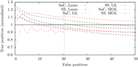
Figure 1: ROC curve relative to baseline, by regime and algorithm. Results are averaged over all data sets. Beyond 20 false positives, only data sets with at least 500 data points and input variables are considered.

For all algorithms, we see that the power is improved by stability selection and screen and clean with respect to the baseline in the critical scenario when the NFP is small, except for group lasso with screen and clean. Also, for small NFP, stability selection outperforms screen and clean. Importantly, stability selection performs consistently well across data configurations. When the NFP is 0, stability selection outperforms the baseline in 51/56 configurations for lasso, 42/56 configurations for group lasso and 21/26 configurations for SIOL. There are only four configurations across all algorithms where stability selection finds less than 70% as many false positives as the baseline.

A breakdown of results by configuration for the case $NFP=0$ is given in section D. While stability selection consistently outperforms the baseline, screen and clean behaves more erratically. Surprisingly, the performance gap between regimes can change significantly between data configurations that are very similar. It is not clear which factors in the data cause each regime to perform well or badly.

As the NFP increases, the performance of stability selection and screen and clean decline with respect to the baseline, suggesting it is more advantageous to use these regimes when we are looking to obtain a small model size. Stability selection still outperforms screen and clean for larger values of NFP for lasso and group lasso, and underperforms for SIOL.

We hypothesize that one reason for the difference in performance between stability selection and screen and clean is that screen and clean does not use group information during the clean phase, as it simply performs least squares regression. This is a disadvantage for detecting weak associations of input variables that share a group with other, more strongly associated input variables. Such variables may be discarded in the clean phase, whereas they may be “saved” by the group structure under the other regimes. This disadvantage is particularly strong for the group lasso, as the penalties are completely group-based. On the other hand, discarding group information in the clean phase is an advantage when it comes to discarding negatives that share a group with one or more positives. This advantage appears if there are groups which are partially contained in $S^{*}$, as in our setup for SIOL.

5.2 Reliability of the theoretical NFP bound

To study whether the NFP bound for stability selection holds in practice, we simply verify whether $\mathcal{\hat{B}}$ exceeds $V$. Of course, this will not always hold. We only have a bound on the expected number of false positives, where the expectation is taken over random draws of the data set. Also, the assumptions required for the bound may be more or less unrealistic, depending on the data and algorithm.

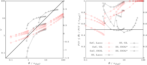
Figure 2: Observed number of false positives against theoretical upper bound, by regime and algorithm. On the left, we show the average number of false positives over all data sets. On the right, we show the probability that $V$ is below the theoretical upper bound. Notice the use of log scales. For $\pi_{SaC}>10$, we only consider data sets with at least 500 input variables and data points. For SIOL with stability selection, we show two curves, one where $\lambda$ is set to achieve $\hat{q}\approx\sqrt{0.8*|K|}$, and one where it is set to achieve $\hat{q}\approx\sqrt{0.8*|K|*t}$.

In section 5.1, we showed that overall, stability selection has high power when setting $\lambda$ to achieve $\hat{q}\approx\sqrt{0.8|K|}$. We will continue to use this heuristic in this section. In figure 2, we show the average number of false positives $V$ obtained under stability selection and the probability of obtaining a number of false positives less than or equal to $\mathcal{\hat{B}}$. The averages / probabilities are with respect to all data sets. The value of $\mathcal{\hat{B}}$ when varying $\pi$ is shown on the x-axis. We also show equivalent results for screen and clean, where the value of the selection threshold $\pi_{SaC}$ itself acts as the bound on the expected NFP, because screen and clean assigns a p-value to each input-output pair.

First, notice that if $\hat{q}\approx\sqrt{0.8|K|}$, $\mathcal{\hat{B}}$ can only lie, approximately, within the range $[0.8,10]$. This is because $\mathcal{\hat{B}}=\frac{\hat{q}^{2}}{|K|(2\pi-1)}\approx\frac{0.8|K|}{|K|(2\pi-1)}=\frac{0.8}{2\pi-1}$. $\pi$ can vary meaningfully between $1$ and just above $0.5$, which leads to the aforementioned range of $\mathcal{\hat{B}}$.

Regime	Algorithm	$\mathcal{\hat{B}}$ / $\pi_{SaC}$	A	B	C	D	E	F	G
SaC	lasso	1	0.07	0.66	3.55	0.76	2.23	2.56	1.11
SS	lasso	1	0.00	0.02	0.03	0.04	0.51	1.04	0.05
SaC	lasso	10	0.67	2.82	8.24	2.31	5.20	4.07	2.73
SS	lasso	10	0.43	1.62	1.60	1.79	4.82	4.20	1.61
SaC	group lasso	1	0.03	0.44	0.22	0.79	2.67	0.59	0.14
SS	group lasso	1	0.00	0.07	0.13	0.99	4.21	1.31	0.45
SaC	group lasso	10	0.28	2.62	1.98	2.46	6.14	1.53	0.55
SS	group lasso	10	0.14	2.34	3.54	4.34	11.70	5.32	3.16
SaC	SIOL	1	0.05	0.72	0.19	2.70	7.88	0.87	0.03
SS	SIOL	1	0.00	0.00	0.00	5.93	9.28	12.95	7.98
SaC	SIOL	10	0.47	3.15	1.54	6.48	17.11	2.31	0.32
SS	SIOL	10	0.01	0.79	0.00	18.31	24.05	28.44	23.15
SS*	SIOL	5	0.01	1.02	0.05	11.39	23.96	27.00	23.46
SS*	SIOL	50	0.53	16.33	7.17	38.89	59.27	61.41	43.89

Table 1: Average number of false positives observed ($V$) by design matrix type when setting the NFP bound to a certain value by tuning $\pi$. For stability selection, we use the heuristic $\hat{q}\approx\sqrt{0.8|K|}$ to set $\lambda$, except rows marked with * use $\hat{q}\approx\sqrt{0.8|K|t}$.

Our results are in line with our hypothesis from section 3 that more complex structure leads to a decline in the error control capabilities of stability selection. We chose our data sets / group structure to make SIOL more challenging than group lasso under the criteria discussed in section 3. When $\mathcal{\hat{B}}=1$, the average number of false positives obtained is 0.20 for lasso, 1.27 for group lasso and 4.95 for SIOL. This result for SIOL becomes 5.64 when the group penalty is multiplied by 2 relative to the individual-component penalty and 4.44 in the reverse case. As expected, a relatively larger group penalty leads to a less reliable NFP bound.

Interestingly, even for SIOL, the probability of exceeding the bound across all data sets never falls significantly below 0.5. In other words, the median of $V$ only exceeds $\mathcal{\hat{B}}$ slightly. This indicates that the distribution of the number of false positives is very sparse across data sets. In fact, setting $\mathcal{\hat{B}}=1$ yields an average of 12.95 false positives for design matrix type (F) and less than 0.01 false positives for design matrix types (A), (B) and (C). Hence, $\mathcal{\hat{B}}$ is not only unreliable for SIOL, but it may be either a gross underestimate or overestimate depending on the data. The complete breakdown by design matrix type is shown in table 1.

A possible reason for this volatility is that large blocks of overlapping groups often mean that either no negatives or a large number of negatives are selected. In our experiments with SIOL, we often saw that $V$ suddenly jumps from 0 to 10 or 15 as $\pi$ decreases. As we cannot feasibly set $\mathcal{\hat{B}}$ to 15, this poses a problem for the usability of the NFP bound. For this reason, we also generated results for the alternative heuristic $\hat{q}\approx\sqrt{0.8|K|t}$. This causes $\mathcal{\hat{B}}$ to lie in the range $[0.8t,10t]$, which is a natural choice for problems with multiple output variables. We show the results in figure 2 and table 1 and observe that the problems are only slightly mitigated. For design matrix types (E) and (F), we still have $V>>\mathcal{\hat{B}}$ and for design matrix types (A), (B) and (C), we still have $V<<\mathcal{\hat{B}}$. This suggests that the pathology is not caused by the choice of $\lambda$.

The accuracy of the NFP bound of screen and clean is affected less by structure and also varies less between design matrix types. Hence, screen and clean may be a better choice for error control when complex structure is present or the data set is challenging. Note that while the threshold $\pi_{SaC}$ can be meaningfully set outside the range $[0.8,10]$ (as opposed to $\mathcal{\hat{B}}$), figure 2 shows that the bound is of poor quality in that region.

5.3 Model Choice

In this section, we investigate the usefulness of the NFP bound of stability selection for automatic parameter tuning as outlined in section 3.1. We will study the very simple objective function $v(T,V)=T-V$, that can be approximated as $\hat{v}(|S|,\mathcal{\hat{B}})=|S|-2*\mathcal{\hat{B}}$. While this objective function has shortcomings (in our most challenging data sets, it is maximized by the empty selection …) it is simple and there does not exist a single objective function that is “right” in all practical situations.

Error Control Scheme	Lasso : True Positives	Lasso : False Positives	GL : True Positives	GL : False Positives	SIOL : True Positives	SIOL : False Positives
SaC	3.74 (4.54)	1.56 (0.38)	4.41 (12.36)	1.19 (3.17)	19.64 (62.06)	2.97 (19.65)
SS (fixed $\lambda$)	3.10 (4.48)	0.75 (0.41)	7.02 (13.55)	3.84 (2.03)	19.86 (62.32)	12.02 (21.78)
SS	3.48 (6.46)	1.59 (0.61)	10.63 (23.94)	5.14 (2.45)	69.12 (122.40)	57.09 (37.47)
Cross-val.	7.30 (4.21)	14.00 (0.75)	20.79 (16.53)	18.58 (3.39)	129.41 (82.58)	144.45 (33.98)

Table 2: Selections obtained from maximizing objective function $v(T,V)=T-V$. We show NTP and NFP obtained from empirical estimates and the “true optima” in brackets. Results are averaged over all data sets.

In table 2, we show the number of true positives and false positives at the parameter configuration where the objective function is maximized, both using proxies and using the actual values for $V$ and $T$. (The latter are shown in brackets.) We find that both stability selection (with $\lambda$ fixed to achieve $\hat{q}\approx\sqrt{0.8|K|}$) and screen and clean find points close to the optimum for lasso, but their performance degrades for the group lasso, and substantially for SIOL. This is no surprise given that we showed that with more complex structure, it becomes harder to estimate the number of false positives. Also, we cannot expect to get close to the optimum if the NFP there exceeds 10. One option for mitigating this is to optimize the objective with respect to both $\lambda$ and $\pi$ under stability selection (line 3 in table 2). While optimizing over too many parameters may lead to over-fitting, we do find significantly more positives for SIOL.

For all algorithms, we notice that stability selection and screen and clean do allow us to find model sizes where the majority of selected variables are true positives. This cannot be achieved by cross-validation, where in 63% of all data configurations, more negatives than positives are selected. Screen and clean seems to be particularly suited for this. For SIOL, only 2.97 negatives are selected on average. We may be able to adjust our objective function to encourage small model sizes and achieve an even better ratio between the number of positives and negatives selected. Cross-validation, on the other hand, should be used for obtaining large selections that contain many positives and negatives, possibly for further processing (as is done inside the screen and clean algorithm). In this regard, the error control schemes complement each other.

6 Discussion and Conclusion

In this paper, we studied the interaction of stability selection  with structured selection algorithms. We found that stability selection raises the statistical power in the critical case when there are few false positives, in most of the settings considered. Hence, even in the absence of error control requirements, it may be preferable to run stability selection. If the selection algorithm uses no structure or the structure is simple, the NFP bound can be used to estimate the number of false positives and set tuning parameters automatically to find a model size where the majority of selected variables are true positives. Such model sizes cannot be found using cross-validation. However, cross-validation excels at selecting large model sizes that contain the majority of positives.

In settings with complex structure (SIOL), the error control mechanisms or stability selection are inaccurate and we found screen and clean to be a better alternative that offers very similar benefits.

This paper has two major caveats. First, it depends heavily on heuristics. Our strategy for setting $\lambda$ and our choice of objective function in section 5.3 are the most prominent examples. There is no guarantee that some of the limitations found in this paper cannot be overcome by better heuristics. Our goal in this paper was to explore one set of heuristics in depth. We hope this paper can serve as a starting point for exploring other heuristics.

The second caveat is that it is difficult to make generalized statements about algorithms like SIOL from studying a finite number of data sets and a small set of group structures. While we conducted a large number of experiments, more work remains to be done to determine which properties of the data sets are responsible for variations in performance between data sets and regimes.

Algorithm	Design matrix type	N	d	s	snr
lasso	A	100	1000	4	0.5
lasso	A	100	1000	4	2
lasso	A	100	1000	10	0.5
lasso	A	100	1000	10	2
lasso	A	1000	1000	20	0.5
lasso	A	1000	1000	20	2
lasso	A	1000	1000	50	0.5
lasso	A	1000	1000	50	2
lasso	B	200	1000	4	0.5
lasso	B	200	1000	4	2
lasso	B	200	1000	10	0.5
lasso	B	200	1000	10	2
lasso	B	1000	1000	20	0.5
lasso	B	1000	1000	20	2
lasso	B	1000	1000	50	0.5
lasso	B	1000	1000	50	2
lasso	C	200	1000	4	0.5
lasso	C	200	1000	4	2
lasso	C	200	1000	10	0.5
lasso	C	200	1000	10	2
lasso	C	1000	1000	20	0.5
lasso	C	1000	1000	20	2
lasso	C	1000	1000	50	0.5
lasso	C	1000	1000	50	2
lasso	D	200	100	10	0.5
lasso	D	200	100	10	2
lasso	D	200	100	30	0.5
lasso	D	200	100	30	2
lasso	D	200	1000	4	0.5
lasso	D	200	1000	4	2
lasso	D	200	1000	10	0.5
lasso	D	200	1000	10	2
lasso	D	1000	1000	20	0.5
lasso	D	1000	1000	20	2
lasso	D	1000	1000	50	0.5
lasso	D	1000	1000	50	2
lasso	E	200	200	10	0.5
lasso	E	200	200	10	2
lasso	E	200	200	30	0.5
lasso	E	200	200	30	2
lasso	E	200	1000	4	0.5
lasso	E	200	1000	4	2
lasso	E	200	1000	10	0.5
lasso	E	200	1000	10	2
lasso	E	1000	1000	20	0.5
lasso	E	1000	1000	20	2
lasso	E	1000	1000	50	0.5
lasso	E	1000	1000	50	2
lasso	F	1000*	5000*	20	0.5
lasso	F	1000*	5000*	20	2
lasso	F	1000*	5000*	50	0.5
lasso	F	1000*	5000*	50	2
lasso	G	114*	1260*	4	0.5
lasso	G	114*	1260*	4	2
lasso	G	114*	1260*	10	0.5
lasso	G	114*	1260*	10	2

Table 3: Data configurations for data sets for the lasso. Parameters valued marked with a * are intrinsic to the fixed design matrix.

Algorithm	Design matrix type	N	d	s	snr
group lasso	A	100	1000	4	0.5
group lasso	A	100	1000	4	2
group lasso	A	200	1000	10	0.5
group lasso	A	200	1000	10	2
group lasso	A	1000	1000	10	0.5
group lasso	A	1000	1000	10	2
group lasso	A	1000	1000	25	0.5
group lasso	A	1000	1000	25	2
group lasso	B	200	1000	4	0.5
group lasso	B	200	1000	4	2
group lasso	B	200	1000	10	0.5
group lasso	B	200	1000	10	2
group lasso	B	1000	1000	10	0.5
group lasso	B	1000	1000	10	2
group lasso	B	1000	1000	25	0.5
group lasso	B	1000	1000	25	2
group lasso	C	200	1000	4	0.5
group lasso	C	200	1000	4	2
group lasso	C	200	1000	10	0.5
group lasso	C	200	1000	10	2
group lasso	C	1000	1000	10	0.5
group lasso	C	1000	1000	10	2
group lasso	C	1000	1000	25	0.5
group lasso	C	1000	1000	25	2
group lasso	D	200	100	5	0.5
group lasso	D	200	100	5	2
group lasso	D	200	100	15	0.5
group lasso	D	200	100	15	2
group lasso	D	200	1000	4	0.5
group lasso	D	200	1000	4	2
group lasso	D	200	1000	10	0.5
group lasso	D	200	1000	10	2
group lasso	D	1000	1000	10	0.5
group lasso	D	1000	1000	10	2
group lasso	D	1000	1000	25	0.5
group lasso	D	1000	1000	25	2
group lasso	E	200	200	5	0.5
group lasso	E	200	200	5	2
group lasso	E	200	200	15	0.5
group lasso	E	200	200	15	2
group lasso	E	200	1000	4	0.5
group lasso	E	200	1000	4	2
group lasso	E	200	1000	10	0.5
group lasso	E	200	1000	10	2
group lasso	E	1000	1000	10	0.5
group lasso	E	1000	1000	10	2
group lasso	E	1000	1000	25	0.5
group lasso	E	1000	1000	25	2
group lasso	F	1000*	5000*	10	0.5
group lasso	F	1000*	5000*	10	2
group lasso	F	1000*	5000*	25	0.5
group lasso	F	1000*	5000*	25	2
group lasso	G	114*	1260*	2	0.5
group lasso	G	114*	1260*	2	2
group lasso	G	114*	1260*	5	0.5
group lasso	G	114*	1260*	5	2

Table 4: Data configurations for data sets for the group lasso. Parameter values marked with a * are intrinsic to the fixed design matrix.

Algorithm	Design matrix type	N	d	s	snr
SIOL	A	500	500	5	0.5
SIOL	A	500	500	5	2
SIOL	A	500	500	10	0.5
SIOL	A	500	500	10	2
SIOL	B	500	500	5	0.5
SIOL	B	500	500	5	2
SIOL	B	500	500	10	0.5
SIOL	B	500	500	10	2
SIOL	C	500	500	5	0.5
SIOL	C	500	500	5	2
SIOL	C	500	500	10	0.5
SIOL	C	500	500	10	2
SIOL	D	500	500	5	0.5
SIOL	D	500	500	5	2
SIOL	D	500	500	10	0.5
SIOL	D	500	500	10	2
SIOL	E	500	500	5	0.5
SIOL	E	500	500	5	2
SIOL	E	500	500	10	0.5
SIOL	E	500	500	10	2
SIOL	F	1000*	5000*	5	0.5
SIOL	F	1000*	5000*	5	2
SIOL	F	1000*	5000*	20	0.5
SIOL	F	1000*	5000*	20	2
SIOL	G	114*	1260*	2	0.5
SIOL	G	114*	1260*	2	2

Table 5: Data configurations for data sets for SIOL. Parameter values marked with a * are intrinsic to the fixed design matrix.

Appendix A Algorithm Details

A.1 Selection algorithms

The selection algorithms we study are also regression algorithms. They are phrased as convex optimization problems over a parameter $\beta$. We minimize the objective until convergence to obtain an optimal parameter value $\hat{\beta}$. Each component of that parameter corresponds to an input-output pair and hence to an element of the selection set $K$. Hence, we may refer to components of $\beta$, selection set elements and input-output pairs interchangeably. We select an element from $K$ if and only if the corresponding component of $\hat{\beta}$ is non-zero.

A.1.1 Lasso

The lasso is a classic, well-studied algorithm for discovering associations between input variables and a single output variable. Hence, $t=1$ and $K$ and the components  of $\beta$ correspond to the set of input variables. Lasso uses least-squares regression coupled with an $L_{1}$-penalty term on the components of $\beta$. This causes shrinkage which in turn leads to components corresponding to input variables with little or no association to the output to become exactly zero. The formula is given below. $\beta$ is a $d$ by $1$ vector.

$$\min_{\beta}\frac{1}{2N}||y-X\beta||_{2}^{2}+\lambda||\beta||_{1}$$

A.1.2 Group lasso

The group lasso is an extension of the Lasso. It is applied in cases where, instead of selecting individual input variables, we wish to select groups of input variables. Each input variable must belong to exactly one group, and $t=1$ holds. In $\hat{\beta}$, either all components  belonging to the same group are equal to zero or all are non-zero. The group-wise selection property is achieved by imposing an $L_{2}$-norm penalty on each group of components. This penalty is called a group penalty.

$$\min_{\beta}\frac{1}{2N}||y-X\beta||_{2}^{2}+\lambda\sum_{g\in G}\theta_{g}||\beta_{g}||_{2}$$

$\beta$ is a $d$ by $1$ vector. $G$ is the set of groups - a set of subsets of $\{1,..,d\}$ such that all $g\in G$ are disjoint and their union is $\{1,..,d\}$. $\beta_{g}$ is the sub-vector of $\beta$ containing the components  of $\beta$ in $g$. This algorithm has additional tuning parameters $\theta_{g}$ that allow us to weight the penalties applied to different groups. Note that this algorithm reduces to the lasso if every input variable belongs to its own group of size one and the $\theta_{g}$ are all equal to one.

A.1.3 Structured input-output lasso

Structured input-output lasso (SIOL) extends group lasso in several respects. Firstly, it admits multiple output variables. This means that $\beta$ becomes a $d$ by $t$ matrix. Secondly, it admits group penalties across components of $\beta$ corresponding to the same output variable. Thirdly, it admits overlapping groups. Fourthly, it combines $L_{2}$-based group penalties with single-component $L_{1}$-penalties. This allows the algorithm to select isolated elements while encouraging the selection of groups as well as blocks of input and output groups which have a high overlap.

$$\min_{\beta}\frac{1}{2N}||Y-X\beta||_{2}^{2}+\lambda(w\sum_{i=1}^{d}\sum_{j=1}^{t}|\beta_{ij}|+\sum_{g\in G}\sum_{j=1}^{t}\theta_{g}||\beta_{gj}||_{2}+\sum_{i=1}^{d}\sum_{h\in H}\phi_{h}||\beta_{ih}||_{2})$$

$G$ is the set of input groups as before except that input groups do not have to be disjoint and not all input variables have to be in an input group. $\beta_{gj}$ is the sub-vector of matrix $\beta$ of components corresponding to output variable $j$ and input variables in $g$. $H$ / $\beta_{ih}$ are the equivalent to $G$ / $\beta_{gj}$ for output groups. $w$, $\theta_{g}$ and $\phi_{h}$ allow us to weight different penalty terms. Note that if no output groups are chosen, this objective function decomposes over output variables into independent optimization problems. If also no input groups are chosen, the algorithm reduces to the Lasso.

Appendix B Experimental details

Group lasso

We only consider groups of equal size and set the group weights $\theta_{g}$ to 1.

SIOL

We set $\theta_{g}$ / $\theta_{h}$ to be equal to the square root of the size of the corresponding group. This is a popular choice. We run SIOL both with $w=0.5$ and $w=2$. Note that instead of fixing tuning parameters such as the $\theta_{g}$ / $\theta_{h}$ or $w$ in advance, we can use the error control schemes to set some or all of them automatically. This is beyond the scope of this paper. We only tune the parameter $\lambda$ (which represents the overall amount of regularization) along with, for stability selection and screen and clean, the selection threshold $\pi$.

Cross-validation

We compute the cross-validation error for a sequence of values $\lambda_{1},\lambda_{2},..,\lambda_{L}$, where $\lambda_{1}$ is large enough so that the initial selection on the training set is empty. We set $\lambda_{l}=0.98*\lambda_{l-1}$ for $2\leq l\leq L$ and we set $L$ to be very large, so that we consider every sensible choice of $\lambda$. A popular rule of thumb is that cross-validation becomes unreliable once there is an output variable for which the number of selected input variables exceeds one half the number of data points in the training set. This is the “cutoff” value for $L$ that we use in this paper. We use ten folds ($k=10$).

Stability Selection

We follow the example of [15]. We run 100 iterations ($I=100$) and sub-sample one half of the data set at each iteration ($p=\frac{1}{2}$). In many experiments, we use the heuristic of setting $\lambda$ to achieve $\hat{q}\approx\sqrt{0.8*|K|}$. As $\lambda$ decreases, $\hat{q}$ almost certainly increases. Thus, there is usually a unique value or a small range of values of $\lambda$ that exactly achieves $\hat{q}=\sqrt{0.8*|K|}$. In practice, we consider the same sequence of $\lambda$-values as in cross-validation, and then choose the smallest value of $\lambda$ in that sequence for which $\hat{q}>\sqrt{0.8*|K|}$ holds.

Screen and Clean We use 10 top-level data splits ($I=10$). Within each screen phases, we use 10-fold cross-validation as described above.

Appendix C Running time

In this section, we compare the running time of different error control schemes. For each of stability selection, screen and clean and cross-validation, the running time is almost completely determined by the number of times they execute the sub-algorithm. In our experiments, we always observed that the running time was close to the value obtained by multiplying the time it took to run the sub-algorithm once with the number of repetitions. Stability selection executes the sub-algorithm $I$ times, there $I$ is the number of iterations. Screen and clean executes the sub-algorithm $Ik$ times, where $I$ is the number of separate screen / clean phases and $k$ is the number of folds used for the cross-validation sub-routine. Cross-validation executes the sub-algorithm $k$ times.

One minor point is that cross-validation runs the sub-algorithm on almost the entire data set, whereas stability selection and screen and clean use only roughly $\frac{1}{2}$ of the data set in each iteration. Hence, cross-validation may take a little longer on each iteration. This assumes that we set the sub-sampling parameter $p$ to $\frac{1}{2}$ for stability selection. In our experiments, we always did this (consistent with [15]) but we may get away with a smaller value to achieve a speed-up.

Also, note that if we set $\lambda$ to achieve $\hat{q}\approx\sqrt{0.8*|K|}$ for stability selection, then we may not have to run the sub-algorithm for small values of $\lambda$ as we have to do for cross-validation and screen and clean. This may cause a significant speed-up, as it is a well-known fact that lasso and related algorithms converge much more slowly when the value of $\lambda$ is small. In our experiments, we used the same values of $\lambda$ for all error control schemes and did not analyze this further.

In our experiments, we chose $k=10$ and $I=10$ for screen and clean and $I=100$ for stability selection. Hence, screen and clean and stability selection had almost the same running time. These values are consistent with other literature.

The benefit of increasing $I$ and $k$ lies in eliminating random noise obtained from random data splitting. Of course, this means that growing $I$ and $k$ yields diminishing returns. We cannot increase $I$ and $k$ arbitrarily and expect our results to keep improving. We did not investigate this trade-off.

Finally, we note that all runs of the sub-algorithm can be trivially parallelized.

Appendix D Detailed Results

In figures 3, 4, and 5, we show by-configuration results for the statistical power of the regimes. We focus on the important case $NFP=0$ and show the largest possible number of true positives that can be selected. To achieve a fair comparison, for each regime, we maximize $NTP$ over a single tuning parameter. For stability selection, we set $\lambda$ to achieve $\hat{q}\approx\sqrt{0.8*|K|}$ and maximize over $\pi$. For screen and clean, we maximize over $\pi$. For the baseline regime, we maximize over $\lambda$. In the charts, we show the probability that the number of positives we can select without selecting a negative is $\lceil\gamma*s\rceil$ or larger ($s=|S^{*}|$), for $\gamma=0.1$ and $\gamma=0.4$. Probabilities are with respect to randomly drawn data sets within each data configuration and are estimated as empirical averages over the 100 data sets we generated for each configuration. In figure 5, we break down results also by the value of $w$, the tuning parameter in SIOL.

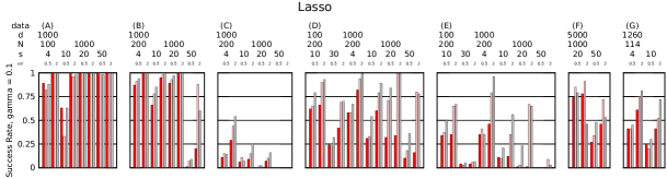
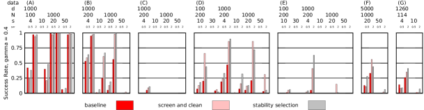
Figure 3: Probability (over 100 random data sets) that there exists a tuning parameter value such that at least $\lceil\gamma*s\rceil$ positives and zero negatives are selected. Parameter values for data configuration are shown above the charts. Results shown pertain to lasso.

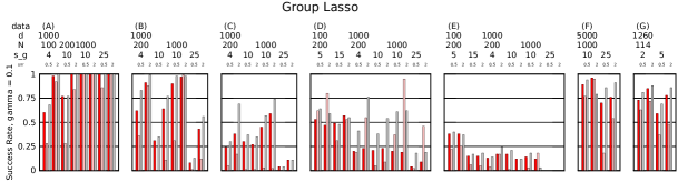
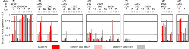
Figure 4: Probability (over 100 random data sets) that there exists a tuning parameter value such that at least $\lceil\gamma*s\rceil$ positives and zero negatives are selected. Parameter values for data configuration are shown above the charts. Results shown pertain to group lasso.

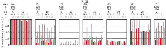
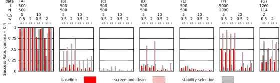
Figure 5: Probability (over 100 random data sets) that there exists a tuning parameter value such that at least $\lceil\gamma*s\rceil$ positives and zero negatives are selected. Parameter values for data configuration are shown above the charts. Results shown pertain to SIOL.

References

- [1] H. Akaike. Information theory and an extension of the maximum likelihood principle. In Proc. Second International Symposium on Information Theory, 1973.
- [2] J. A. Bazerque, G. Mateos, and G. B. Giannakis. Group-lasso on splines for spectrum cartography. Signal Processing, IEEE Transactions on, 59(10):4648–4663, 2011.
- [3] B. Efron. The jackknife, the bootstrap and other resampling plans. In SIAM, 1982.
- [4] R. Jenatton, J. Mairal, F. R. Bach, and G. R. Obozinski. Proximal methods for sparse hierarchical dictionary learning. In Proceedings of the 27th International Conference on Machine Learning (ICML-10), pages 487–494, 2010.
- [5] S. Kim, K. Sohn, and E. Xing. A multivariate regression approach to association analysis of a quantitative trait network. Bioinformatics, 25(12):i204, 2009.
- [6] S. Kim and E. P. Xing. Tree-guided group lasso for multi-task regression with structured sparsity. In Proceedings of the 27th International Conference on Machine Learning, pages 543–550, 2010.
- [7] S. Lee, A. Dudley, D. Drubin, P. Silver, N. Krogan, D. Pe’er, and D. Koller. Learning a prior on regulatory potential from eQTL data. PLoS Genetics, 5(1), 2009.
- [8] S. Lee and E. Xing. Leveraging input and output structures for joint mapping of epistatic and marginal eqtls. In Proc. ISMB, 2012.
- [9] S. Lee and E. P. Xing. Leveraging input and output structures for joint mapping of epistatic and marginal eqtls. Bioinformatics, 28(12):i137–i146, 2012.
- [10] C. Li and M. Li. The landscape of genetic complexity across 5,700 gene expression traits in yeast. PNAS, 102(5):1572–1577, 2005.
- [11] C. Li and M. Li. Gwasimulator: a rapid whole-genome simulation program. Bioinformatics, 24(1):140–142, 2008.
- [12] H. Liu, K. Roeder, and L. Wasserman. Stability approach to regularization selection (stars) for high-dim graphical models. In Advances in Neural Information Processing Systems 23, pages 1432–1440, 2010.
- [13] Z. Lu, B. Savas, W. Tang, and I. S. Dhillon. Supervised link prediction using multiple sources. In Data Mining (ICDM), 2010 IEEE 10th International Conference on, pages 923–928. IEEE, 2010.
- [14] S. Ma, X. Song, and J. Huang. Supervised group lasso with applications to microarray data analysis. BMC bioinformatics, 8(1):60, 2007.
- [15] N. Mainshausen and P. Bühlmann. Stability selection. Journal of the Royal Statistical Society: Series B, 72(4):417–473, 2010.
- [16] N. Meinshausen, L. Meier, and L. Bühlmann. P-values for high-dimensional regression. Journal of the American Statistical Association, 104(488):1671–1681, 2009.
- [17] G. Schwarz. Estimating the dimension of a model. The Annals of Statistics, 6(2):461–464, 1978.
- [18] Z. Szabó, B. Póczos, and A. Lorincz. Online group-structured dictionary learning. In Computer Vision and Pattern Recognition (CVPR), 2011 IEEE Conference on, pages 2865–2872. IEEE, 2011.
- [19] R. Tibshirani. Regression shrinkage and selection via the lasso. Journal of the Royal Statistical Society, Series B, 58(1):267–288, 1996.
- [20] G. Varoquaux, A. Gramfort, J.-B. Poline, B. Thirion, et al. Brain covariance selection: better individual functional connectivity models using population prior. In NIPS, volume 10, pages 2334–2342, 2010.
- [21] J. Wu, B. Devlin, S. Ringquist, M. Trucco, and K. Roeder. Screen and clean: a tool for identifying interactions in genome-wide association studies. Genet Epidemiol., 34(3):275–285, 2010.
- [22] Y. Yang, Y. Yang, Z. Huang, H. T. Shen, and F. Nie. Tag localization with spatial correlations and joint group sparsity. In Computer Vision and Pattern Recognition (CVPR), 2011 IEEE Conference on, pages 881–888. IEEE, 2011.
- [23] M. Yuan and Y. Lin. Model selection and estimation in regression with grouped variables. Journal of the Royal Statistical Society, Series B, 68(1):49–67, 2006.