Cu hyperfine coupling constants of HgBa₂CaCu₂O_6+δ

Abstract

We estimated the ratios of ⁶³Cu hyperfine coupling constants in the double-layer high-$T_{\mathrm{c}}$ superconductor HgBa₂CaCu₂O_6+δ from the anisotropies in Cu nuclear spin-lattice relaxation rates and spin Knight shifts to study the nature of the ultraslow fluctuations causing the $T_{2}$ anomaly in the Cu nuclear spin-echo decay. The ultraslow fluctuations may come from uniform magnetic fluctuations spread around the wave vector $q$ = 0, otherwise the electric origins.

1 Introduction

Spin polarized neutron scattering experiments indicate the emergence of an intra-unit-cell (IUC) $q$ = 0 magnetic moments in the pseudogap states of the high-$T_{\mathrm{c}}$ cuprate superconductors, while no NMR and $\mu$SR experiment indicates any static ordering of local magnetic moments [1]. The IUC moments are associated with the loop current ordered state [2]. Recently discovered ultraslow fluctuations in the pseudogap states of HgBa₂CaCu₂O_6+δ (Hg1212) via ⁶³Cu nuclear spin-echo decay experiments [3] might reconcile an issue on the IUC moments. No wipeout effect on NMR spectra is characteristic of the ultraslow fluctuations of Hg1212, in contrast to the spin-charge stripe orderings [4, 5].

Knowledge of the hyperfine coupling constants helps us to clarify the nature of the local field fluctuations in NMR measurements [6]. In this paper, we report the estimation of the ⁶³Cu hyperfine coupling constants in the double-CuO₂-layer high-$T_{\mathrm{c}}$ superconductors Hg1212 from the anisotropies in ⁶³Cu nuclear spin-lattice relaxation rates and spin Knight shifts [7], and discuss the nature of the ultraslow fluctuations [3].

2 Estimations of ⁶³Cu hyperfine coupling constants

The ⁶³Cu hyperfine coupling parameters ($A_{cc}^{hf}$ and $A_{ab}^{hf}$) consist of the anisotropic on-site $A_{cc}$ (the $c$ axis component) and $A_{ab}$ (the $ab$ plane component) due to the 3$d$ electrons and the isotropic supertransferred component $B(>0)$ [6]. The ratios of the individual components in the three coupling constants can be estimated from the anisotropy data [7] of the ⁶³Cu Knight shifts (${}^{63}K_{cc}$ and ${}^{63}K_{ab}$) and the ⁶³Cu nuclear spin-lattice relaxation rates [(1/$T_{1}$)_cc and (1/$T_{1}$)_ab] via the antiferromagnetic dynamical spin susceptibility [6, 8, 9, 10, 11]. The subscript indices of $cc$ or $ab$ of ${}^{63}K$ and 1/$T_{1}$ indicate the direction of a static magnetic field applied along the $c$ axis or in the $ab$ plane. The procedure to estimate the coupling constant ratios is shown below.

2.1 ⁶³Cu Knight shifts

The ⁶³Cu Knight shifts ${}^{63}K_{cc,ab}$ at a magnetic field along the $c$ axis or in the $ab$ plane are the sum of the spin shift $K_{spin}$ and the orbital shift $K_{orb}$ as ${}^{63}K_{cc,ab}=K_{spin}^{cc,ab}(T)+K_{orb}^{cc,ab}$. The spin shift is $K_{spin}^{cc,ab}(T)=A_{cc,ab}^{hf}\chi_{s}^{cc,ab}(T)$ with the hyperfine coupling parameters $A_{cc,ab}^{hf}$ and the uniform spin susceptibility $\chi_{s}^{cc,ab}(T)$. For a temperature-dependent isotropic spin susceptibility $\chi_{s}^{cc}=\chi_{s}^{ab}$, the ratio $\Delta K_{spin}^{cc}/\Delta K_{spin}^{ab}=(dK_{spin}^{cc}/dT)/(dK_{spin}^{ab}/dT)$ is equal to the ratio $A_{cc}^{hf}/A_{ab}^{hf}$.

Figure 2 shows ${}^{63}K_{cc}$ plotted against ${}^{63}K_{ab}$ with temperature as an implicit parameter for Hg1212 from underdoped to overdoped, which are adopted from [7]. The sold straight lines are the least-squares fitting results. The dashed straight line for overdoped Hg1212 is a visual guide with assuming the same slope as the optimally doped Hg1212. The straight lines show nearly parallel shift. Since the orbital shifts of $K_{orb}^{cc}$ = 1.14$-$1.16 $\%$ and $K_{orb}^{ab}$ = 0.19$-$0.20 $\%$ are estimated below $T_{\mathrm{c}}$, then the parallel shift indicates a constant spin component above $T_{\mathrm{c}}$. Similar parallel shift is found in the single crystal NMR for HgBa₂CuO_4+δ [12].

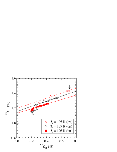
Figure 1: ${}^{63}K_{cc}$ versus ${}^{63}K_{ab}$ with temperature as an implicit parameter for Hg1212 from underdoped to overdoped [7]. The arrows indicate $T_{\mathrm{c}}$.

Figure 2: Anisotropy ratio ⁶³(1/$T_{1}$)_ab/⁶³(1/$T_{1}$)_cc against temperature for Hg1212 from underdoped to overdoped [7].

An easy plane magnetic anisotropy causes such a constant spin component in the paramagnetic spin susceptibility [13]. The anisotropic superexchange interaction in the $S$ = 1/2 XXZ Heisenberg Hamiltonian yields the easy plane anisotropy in the paramagnetic state [14, 15]. The optimally hole doping makes the anisotropy weak [13, 16]. Although the multicomponents in the spin susceptibility are suggested from the anisotropic spin Knight shifts [12, 17], we believe that the doped superconductors with a single spin component can show a finite anisotropy and that the constant spin component does not impede a single spin component analysis to estimate the Cu hyperfine coupling constants.

The ⁶³Cu hyperfine coupling parameters $A_{cc}^{hf}$ and $A_{ab}^{hf}$ are expressed by $A_{cc}$, $A_{ab}$, and $B$ as $A_{cc}^{hf}=A_{cc}+4B$ and $A_{ab}^{hf}=A_{ab}+4B$ [6, 8, 18]. Then, the anisotropy ratio $r_{u}$ of the temperature-dependent $K_{s}^{cc}$ and $K_{s}^{ab}$ is given by

$$r_{u}\equiv{\Delta K_{s}^{cc}\over{\Delta K_{s}^{ab}}}={A_{cc}+4B\over{A_{ab}+4B}}.$$ (1)

Figure 2 shows $r_{u}$ = 0.31 for the underdoped and 0.34 for the optimally doped samples. The value of $r_{u}$ = 0.34 is assumed for the overdoped sample.

2.2 ⁶³Cu nuclear spin-lattice relaxation rate

Figure 2 shows the ratio of ⁶³(1/$T_{1}$)_ab/⁶³(1/$T_{1}$)_cc plotted against temperature for Hg1212 from underdoped to overdoped (adopted from Ref. [7]). The anisotropy ratio $r_{\mathrm{AF}}$ of (1/$T_{1}$)_ab and (1/$T_{1}$)_cc is given by

$$r_{\mathrm{AF}}\equiv{(1/T_{1})_{ab}\over{(1/T_{1})_{cc}}}\approx{1\over 2}\biggl{\{}1+\biggl{(}{A_{cc}-4B\over{A_{ab}-4B}}\biggr{)}^{2}\biggr{\}},$$ (2)

for the leading term of the enhanced antiferromagnetic susceptibility [11]. For convenience, we introduce an alternative parameter of $r_{A}=\sqrt{2r_{\mathrm{AF}}-1}$. We adopted the values of $r_{AF}$ ($r_{A}$) = 2.3 (1.90), 2.0 (1.73), and 1.8 (1.61) from underdoped to overdoped (figure 2) to estimate the coupling constant ratios.

2.3 ⁶³Cu hyperfine coupling constant ratios

From the constraints of $A_{cc}$ $<$ 0 [18] and $A_{ab}/4B$ $<$ 1 on (1) and (2), we obtain the expressions of the ratios of the ⁶³Cu hyperfine coupling constants,

$${A_{cc}\over{4B}}\approx-{{r_{A}+r_{u}-2r_{A}r_{u}}\over{r_{A}-r_{u}}},$$ (3)

$${A_{ab}\over{4B}}\approx{{r_{A}+r_{u}-2}\over{r_{A}-r_{u}}},$$ (4)

and then

$${A_{ab}\over{A_{cc}}}\approx-{{r_{A}+r_{u}-2}\over{r_{A}+r_{u}-2r_{A}r_{u}}}.$$ (5)

Thus, (3)-(5) with a set of $r_{u}$ and $r_{A}$ enable us to estimate the ratios of the ⁶³Cu hyperfine coupling constants.

Table 1: Anisotropies ($r_{u}$ and $r_{AF}$) of ${}^{63}K_{s}$ and ${}^{63}T_{1}$, and the ratios of ⁶³Cu hyperfine coupling constants ($A_{cc}$, $A_{ab}$, $B$) for underdoped (un), optimally doped (op) and overdoped (ov) Hg1212. $T_{\mathrm{c}}$ is in kelvin. The value of $r_{u}$ for overdoped Hg1212 is assumed after the optimally doped value in figure 1.

$\0\0$	$\0T_{\mathrm{c}}$	$\0\0r_{u}$	$r_{AF}$	$A_{cc}/4B$	$A_{ab}/4B$	$A_{ab}/A_{cc}$
un	103	$\0$0.31	2.3	$\0-0.65$	$\0+0.13$	$\0-0.20$
op	127	$\0$0.34	2.0	$\0-0.64$	$\0+0.05$	$\0-0.078$
ov	$\0$93	$\0$0.34	1.8	$\0-0.67$	$\0-0.04$	$\0+0.058$

Table 1 shows the estimated ratios of $A_{cc}/4B$, $A_{ab}/4B$ and $A_{ab}/A_{cc}$ for Hg1212 from (3)-(5) with the experimental $r_{u}$ and $r_{AF}$ in figures 2 and 2. The on-site coupling ratio $A_{ab}/A_{cc}$ depends on the hole concentration in Hg1212.

The 3$d(x^{2}-y^{2})$ orbital electron of Cu²⁺ in the tetragonal crystal field produces the on-site hyperfine fields. The ratio $A_{ab}/A_{cc}$ is expressed as

$${A_{ab}\over{A_{cc}}}\approx-{{-\kappa+{{2}\over{7}}-{{11}\over{7}}\gamma}\over{-\kappa-{{4}\over{7}}-{{62}\over{7}}\gamma}},$$ (6)

where $\kappa$($>$ 0) is the core polarization parameter, 2/7 and $-$4/7 are the spin-dipole field coefficients, and $\gamma$($<$ 0) is the spin-orbit coupling parameter [9, 19, 20]. The empirical values of $\kappa$ = 0.25 and 0.325 were estimated for Cu²⁺ ions in the dilute copper salts [20]. The first-principles cluster calculations give $\kappa$ = 0.289 for the density functional $<1/r^{3}>$ and 0.455 for the Hartree-Fock $<1/r^{3}>$ in La₂CuO₄ [21]. The value of $\kappa$ = 0.41 is found in CuGeO₃ [22]. For Hg1212, $A_{ab}/A_{cc}$ in Table 1 through (6) leads to the core polarization parameter $\kappa$ = 0.265 (un), 0.315 (op) and 0.387 (ov), assuming $\gamma$ = $-$0.044 [9, 19].

2.4 ⁶³Cu hyperfine coupling constants of HgBa₂CuO_4+δ and Hg1212

Let us show the ⁶³Cu hyperfine coupling constants of the optimally doped single-CuO₂-layer superconductor HgBa₂CuO_4+δ ($T_{\mathrm{c}}$ = 98 K). From the uniform spin susceptibility $\chi_{s}$ = 1.47$\times$10^-4 emu/mole-f.u. [23] and the in-plane ⁶³Cu $K_{spin}^{ab}$ = 0.48 $\%$ [24], we estimated the in-plane ⁶³Cu hyperfine coupling parameter $A_{ab}^{hf}$ = $A_{ab}+4B$ = ($N_{\mathrm{A}}\mu_{\mathrm{B}}/\chi_{s})K_{spin}^{ab}$ = 182 kOe/$\mu_{\mathrm{B}}$ for HgBa₂CuO_4+δ ($N_{\mathrm{A}}$ is Avogardro’s number and $\mu_{B}$ is the Bohr magneton). Substituting $r_{u}$ = 0.53 and $r_{AF}$ = 1.8 [24] into (3)-(5) and using $A_{ab}$ + 4$B$ = 182 kOe/$\mu_{\mathrm{B}}$, we obtained the values of

$A_{cc}$ = $-$ 65, $A_{ab}$ = 21, and $B$ = 40 kOe/$\mu_{B}$

for the optimally doped HgBa₂CuO_4+δ.

Table 2: ⁶³Cu hyperfine coupling constants in units of kOe/$\mu_{\mathrm{B}}$ for underdoped (un), optimally doped (op) and overdoped (ov) Hg1212, assuming $A_{ab}+4B$ = 182 kOe/$\mu_{\mathrm{B}}$.

$\0\0$	$A_{cc}$	$A_{ab}$	$B$
un	$-105$	$+21$	$40$
op	$-111$	$+8.7$	$43$
ov	$-127$	$-7.4$	$47$

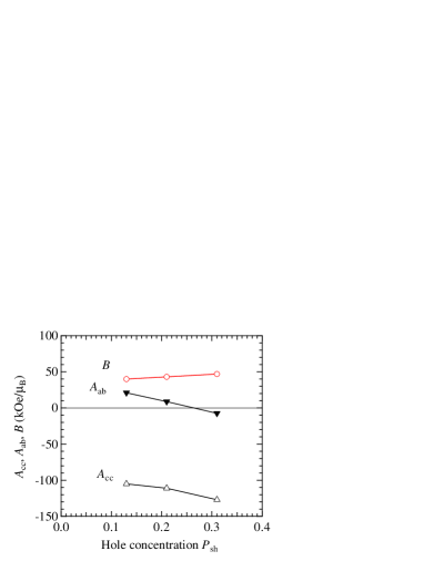
Figure 3: ⁶³Cu hyperfine coupling constants $A_{cc}$, $A_{ab}$, and $B$ plotted against hole concentration $P_{sh}$ for Hg1212. The solid curves are visual guides.

By adopting $A_{ab}+4B$ = 182 kOe/$\mu_{\mathrm{B}}$ for Hg1212 after HgBa₂CuO_4+δ, we estimated the individual components of $A_{cc}$, $A_{ab}$, and $B$ (Table 2). Figure 3 shows $A_{cc}$, $A_{ab}$, and $B$ (Table 2) plotted against the hole concentration $P_{sh}$ [7] for Hg1212. In Table 2 and figure 3, with increase in the hole concentration, the absolute value of the negative $A_{cc}$ increases, $A_{ab}$ shows a sign change, and the $B$ term slightly increases.

The reported $B$ term is in the range from 36 to 155 kOe/$\mu_{\mathrm{B}}$ in the other cuprate superconductors  [10, 25, 26, 27, 28], assuming a priori the fixed values of $A_{cc}$ = $-$170 and $A_{ab}$ = 37 kOe/$\mu_{\mathrm{B}}$ [25, 27, 28]. The cation-cation supertransferred hyperfine field $B$ between 3$d$ and 4$s$ orbitals depends on the strength of the $p$-$d$ covalent bond parameter [29]. The doping dependent $B$ term in Table 2 indicates the development of the covalency with the hole concentration in Hg1212.

3 Local field fluctuations in ⁶³Cu nuclear spin-echo decay rate 1/$T_{2L}$

3.1 ⁶³Cu nuclear spin-echo decay rate 1/$T_{2L}$

Figures 4(a)-4(c) show the ⁶³Cu nuclear spin-echo decay rates (1/$T_{\mathrm{2L}}$)_ab,cc’s for Hg1212 from underdoped (a), optimally doped (b) and overdoped (c) [3]. The notations conform to those in [3]. The enhancements in (1/$T_{\mathrm{2L}}$)${}_{ab,~{}cc}$ at 220$-$240 K indicate the ultraslow fluctuations [3]. The peak temperature of (1/$T_{\mathrm{2L}}$)_cc is nearly independent of the doping level, but the enhancement is suppressed by overdoping.

Figure 4(d) shows the anisotropy ratio of the local field fluctuations $\Delta J_{cc}/\Delta J_{ab}$ $\equiv$ [(1/$T_{\mathrm{2L}}$)_cc $-$ (1/$T_{\mathrm{2R}}$)_cc]/[(1/$T_{\mathrm{2L}}$)_ab $-$ (1/$T_{\mathrm{2R}}$)_ab] derived from 1/$T_{\mathrm{2L}}$ and 1/$T_{1}$ (Redfield’s 1/$T_{\mathrm{2R}}$) [3]. $\Delta J_{\gamma\gamma}$ ($\gamma\gamma$ = $cc$ and $ab$) expresses the additional fluctuations causing the enhancement in 1/$T_{\mathrm{2L}}$. One should note that $\Delta J_{cc}/\Delta J_{ab}<$ 1 is characteristic of the ultraslow fluctuations.

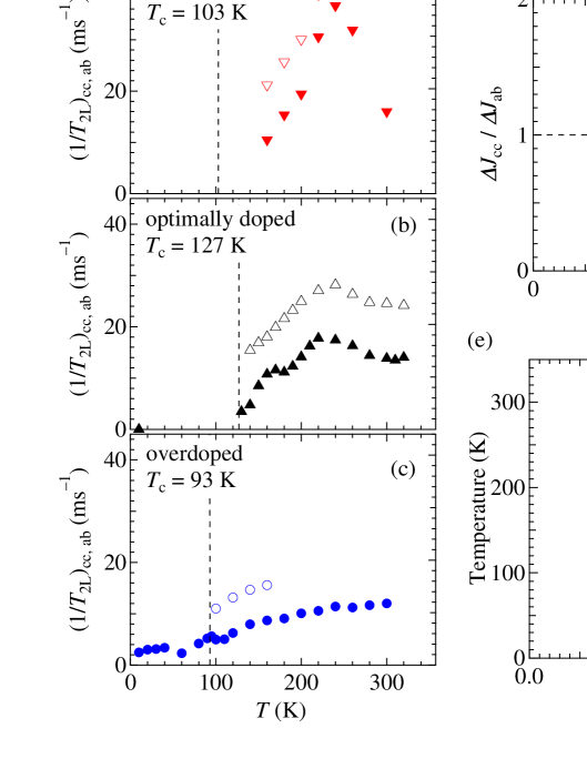
Figure 4: (a)$-$(c) $T$ dependences of (1/$T_{\mathrm{2L}}$)_cc (closed symbols) and (1/$T_{\mathrm{2L}}$)_ab (open symbols) from underdoped to overdoped Hg1212 [3]. Each dashed line indicates $T_{\mathrm{c}}$. (d) $T$ dependences of $\Delta J_{cc}/\Delta J_{ab}$ [3]. (e) Phase diagram of Hg1212: $T_{\mathrm{c}}$ (closed circles), the pseudo spin-gap temperature defined by the maximum temperature of 1/$T_{1}T$ [7] (closed squares), $T_{\mathrm{p}}$ defined by the peak temperature of (1/$T_{\mathrm{2L}}$)_cc [3] (open triangles) against hole concentration $P_{sh}$. The dotted curve with a shaded region is a visual guide for the onset temperature $T^{*}$ of decrease in ⁶³Cu Knight shift [7]. Nearly AF stands for the Curie-Weiss law in Cu 1/$T_{1}T$ [7].

Figure 4(e) shows the phase diagram of Hg1212, where the superconducting transition temperature $T_{\mathrm{c}}$, the pseudo spin-gap temperature defined by the maximum temperature of 1/$T_{1}T$, $T_{\mathrm{p}}$ defined by the peak temperature of (1/$T_{\mathrm{2L}}$)_cc, and the onset temperature $T^{*}$ of the decrease in the Cu Knight shift are plotted against the hole concentration $P_{sh}$ in Cu${}^{2+P_{sh}}$ [3, 7]. With hole doping, $T^{*}$ decreases, while $T_{\mathrm{p}}$ is nearly independent of the hole concentration $P_{sh}$. The ultraslow fluctuations emerge in the underdoped regime and diminish in the overdoped regime.

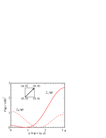
Figure 5: ⁶³Cu hyperfine coupling form factors $f_{cc}$($q$) and $f_{ab}$($q$) as functions of $q$ in the wave vector $q$ = ($q$, $q$) [(0, 0) $\rightarrow$ ($\pi$, $\pi$)]. Inset shows the diagonal in the first Brillouin zone.

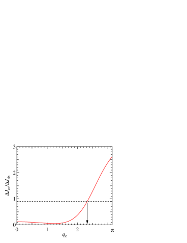
Figure 6: $\Delta J_{cc}/\Delta J_{ab}$ as a function of the cut off $q_{c}$ in a toy model upon a static spin susceptibility $\chi^{\prime}({\mbox{\boldmath$q$}})$ = $\chi_{0}^{\prime}$ ($\left|q_{x,y}\right|<q_{c}$) and 0 ($\left|q_{x,y}\right|>q_{c}$). Experimental constraint leads to $q_{c}$ $<$ 2.3.

3.2 Local field fluctuations

Local field fluctuations of $J_{ab}$ ($B\perp$c axis) and $J_{cc}$ ($B\parallel$c axis) causing the nuclear spin relaxations of $T_{1}$ and $T_{2}$ are defined by

$$J_{\gamma\gamma}=\sum_{\mbox{\boldmath$q$}}F_{\gamma\gamma}({\mbox{\boldmath$q$}})S({\mbox{\boldmath$q$}},\nu_{n}),$$ (7)

$$F_{\gamma\gamma}({\mbox{\boldmath$q$}})\equiv(4B)^{2}f_{\gamma\gamma}({\mbox{\boldmath$q$}})=[A_{\gamma\gamma}+2B\{\mathrm{cos}(q_{x})+\mathrm{cos}(q_{y})\}]^{2},$$ (8)

where $\gamma\gamma$ = $ab$ and $cc$, and $\nu_{n}$ is an NMR frequency [3]. The electron spin-spin correlation function $S$($q$, $\nu$) (a frequency $\nu$) is related to the dynamical spin susceptibility $\chi^{\prime\prime}$($q$, $\nu$) through the fluctuation-dissipation theorem. $F_{\gamma\gamma}$($q$) is called the form factor of the wave vector $q$ dependent hyperfine coupling constant, whose filtering effects in the $q$ space play a significant role in the anisotropy and the site differentiation on NMR [8, 9, 10]. $\Delta J_{\gamma\gamma}$ expresses the additional fluctuations to $J_{\gamma\gamma}$ [3].

Figure 6 shows the $q$ dependence of $f_{ab,~{}cc}$($q$) for Hg1212 along the diagonal $q$ = ($q$, $q$) in the first Brillouin zone, using the estimated coupling constant ratios in Table 1. Since $f_{cc}$($\pi$, $\pi$) $>$ $f_{ab}$($\pi$, $\pi$), the antiferromagnetic spin fluctuation $\chi^{\prime}$($q$) localized around $q$ = [$\pi$, $\pi$] leads to the anisotropy $J_{cc}/J_{ab}\sim$ 3 in contrast to the experimental ratio $\Delta J_{cc}/\Delta J_{ab}<$ 1 in figure 4(d) [3]. $\Delta J_{\gamma\gamma}$ expresses the development of the ultraslow fluctuations [3]. Thus, the antiferromagnetic fluctuations are excluded from the ultraslow fluctuations.

Let us assume a toy model of $\chi^{\prime}$($q$, $\nu_{n}$) = $\chi^{\prime}_{0}\Theta(q_{c}-\left|q_{x}\right|)\Theta(q_{c}-\left|q_{y}\right|)$ ($\Theta(x)$ is the Heaviside step function). $q_{c}$ is a cut-off wave number. $\chi^{\prime}({\mbox{\boldmath$q$}})$ $\propto$ $S$($q$, $\nu_{n}$) takes a constant value $\chi^{\prime}_{0}$ over $\left|q_{x,y}\right|<q_{c}$. For this toy model, the ratio $\Delta J_{cc}/\Delta J_{ab}$ is calculated as

$${\Delta J_{cc}\over{\Delta J_{ab}}}={{\sum_{\left|q_{x,y}\right|<q_{c}}f_{cc}({\mbox{\boldmath$q$}})}\over{\sum_{\left|q_{x,y}\right|<q_{c}}f_{ab}({\mbox{\boldmath$q$}})}}.$$ (9)

Figure 6 shows the numerical $\Delta J_{cc}/\Delta J_{ab}$ as a function of $q_{c}$. The experimental $\Delta J_{cc}/\Delta J_{ab}$ $<$ 0.9 in figure 4(d) imposes on the function in figure 6 and then leads to $q_{c}$ $<$ 2.3. The magnetic ultraslow fluctuations must be confined within $q_{c}$ $<$ 2.3. If the magnetic ultraslow fluctuations have the easy plane anisotropy, the upper limit of the cut-off value $q_{c}$ will be smaller than 2.3. Thus, we obtained a model constraint on the magnetic ultraslow fluctuations, using the anisotropic hyperfine coupling constants.

Although the step function $\chi^{\prime}({\mbox{\boldmath$q$}})$ with $q_{c}$ $<$ 2.3 is not localized at $q$ = 0, it is parallel to the IUC $q$ = 0 magnetic moments observed by the spin polarized neutron scattering method [1]. The ultraslow fluctuations may be associated with the IUC $q$ = 0 magnetic moments. However, if the enhancement in 1/$T_{\mathrm{2L}}$ is due to quadrupole fluctuations, one should explore the alternative fluctuations of charge or lattice for the electric ultraslow fluctuations.

4 Conculsions

The systematic hole doping dependences of the ⁶³Cu hyperfine coupling constants ($A_{cc}$, $A_{ab}$ and $B$) were found for Hg1212 from underdoped to overdoped. A model constraint on the magnetic ultraslow fluctuations in Hg1212 was derived from the anisotropy ratios of the ⁶³Cu hyperfine coupling constants. The model expresses the magnetic fluctuations spread around $q$ = 0. Possible electric ultraslow fluctuations causing the $T_{2}$ anomaly remain to be explored.

We thank Jun Kikuchi for fruitful discussions on the hyperfine coupling constants.

References

References

- [1] Bourges P and Sidis Y 2011 C. R. Physique 12 461
- [2] Varma C M 2014 J. Phys.: Condens. Matter 26 505701
- [3] Itoh Y, Machi T and Yamamoto A 2017 Phys. Rev. B 95 094501
- [4] Singer P M, Hunt A W, Cederström A F and Imai T 1999 Phys. Rev. B 60 15345
- [5] Hunt A W, Singer P M, Cederström A F and Imai T 2001 Phys. Rev. B 64 134525
- [6] Mila F and Rice T M 1989 Physica C 157 561
- [7] Itoh Y, Tokiwa-Yamamoto A, Machi T and Tanabe K 1998 J. Phys. Soc. Jpn. 67 2212
- [8] Millis A J, Monien H and Pines D 1990 Phys. Rev. B 42 167
- [9] Monien H, Pines D and Slichter C P 1990 Phys. Rev. B 41 11120
- [10] Imai T 1990 J. Phys. Soc. Jpn. 59 2508
- [11] Itoh Y, Hayashi A and Ueda Y 1995 J. Phys. Soc. Jpn. 64 3074
- [12] Rybicki D, Kohlrautz J, Haase J, Greven M, Zhao X, Chan M K, Dorow C J and Veit M J 2015 Phys. Rev. B 92 081115
- [13] Shimizu T, Aoki H, Yasuoka H, Tsuda T, Ueda Y, Yoshimura K and Kosuge K 1993 J. Phys. Soc. Jpn. 62 3710
- [14] Hanzawa K 1994 J. Phys. Soc. Jpn. 63 264
- [15] Okabe Y and Kikuchi M 1988 J. Phys. Soc. Jpn. 57 4751
- [16] Terasaki I, Hase M, Maeda A, Uchinokura K, Kimura T, Kishio K, Tanaka I and Kojima H 1992 Physica C 193 365
- [17] Haase J, Jurkutat M, Kohlrautz J 2017 Condense. Matter 2 16
- [18] Takigawa M, Hammel P C, Heffner R H, Fisk Z, Smith J L and Schwarz R B 1989 Phys. Rev. B 39 300
- [19] Pennington C H, Durand D J, Slichter C P, Rice J P, Bukowski E D and Ginsberg D M 1989 Phys. Rev. B 39 2902
- [20] Bleaney B, Bowers K D and Pryce M H L 1955 Proc. Roy. Soc. London, Ser. A 228 166
- [21] Hüsser P, Suter H U, Stoll E P and Meier P F 2000 Phys. Rev. B 61 1567
- [22] Itoh M, Sugahara M, Yamauchi T and Ueda Y 1996 Phys. Rev. B 53 11606
- [23] Itoh Y, Machi T and Yamamoto A [arXiv:2091155]
- [24] Itoh Y, Machi T, Adachi S, Fukuoka A, Tanabe K and Yasuoka H 1998 J. Phys. Soc. Jpn. 67 312
- [25] Kitaoka Y, Fujiwara K, Ishida K, Asayama K, Shimakawa Y, Manako T and Kubo Y 1991 Physica C 179 107
- [26] Kambe S, Yasuoka H, Hayashi A and Ueda Y 1993 Phys. Rev. B 47 2825
- [27] Ishida K, Kitaoka Y, Asayama K, Kadowaki K and Mochiku T 1994 J. Phys. Soc. Jpn. 63 1104
- [28] Shimizu S, Iwai S, Tabata S-I, Mukuda H, Kitaoka Y, Shirage P M, Kito H and Iyo A 2011 Phys. Rev. B 83 144523
- [29] Huang N L, Orbach R, Šimánek E, Owen J and Taylor D R 1967 Phys. Rev. 156 383