Modeling Radio Circular Polarization in the Crab Nebula

Abstract

In this paper we present, for the first time, simulated maps of the circularly polarized synchrotron emission from the Crab nebula, using multidimensional state of the art models for the magnetic field geometry. Synchrotron emission is the signature of non-thermal emitting particles, typical of many high-energy astrophysical sources, both Galactic and extra-galactic ones. Its spectral and polarization properties allow us to infer key informations on the particles distribution function and magnetic field geometry. In recent years our understanding of pulsar wind nebulae has improved substantially thanks to a combination of observations and numerical models. A robust detection or non-detection of circular polarization will enable us to discriminate between an electron-proton plasma and a pair plasma, clarifying once for all the origin of the radio emitting particles, setting strong constraints on the pair production in pulsar magnetosphere, and the role of turbulence in the nebula. Previous attempts at measuring the circular polarization have only provided upper limits, but the lack of accurate estimates, based on reliable models, makes their interpretation ambiguous. We show here that those results are above the expected values, and that current polarimetric tecniques are not robust enough for conclusive result, suggesting that improvements in construction and calibration of next generation radio facilities are necessary to achieve the desired sensitivity.

1 Introduction

Pulsar wind nebulae (PWNe) form when the relativistic wind from a pulsar interacts with the environment (either the ISM or the parent supernova remnant), leading to the formation of a synchrotron emitting bubble, that shines in a broad range of frequencies from radio wavelengths to $\gamma$-rays (see Gaensler & Slane 2006 for a review). Among PWNe, the Crab nebula (Hester, 2008) plays a special role. It is perhaps one of the most studied object in the sky: we know its birth date, and the spin down properties of the central pulsar (Lyne, Pritchard & Graham-Smith, 1993); we have good estimates for the mass of the progenitor (the mass of the confining ejecta) (MacAlpine & Satterfield, 2008); its spectrum as been observed from low radio frequencies (Baldwin, 1971; Baars, 1972), through mm/IR (Mezger et al., 1986; Bandiera, Neri & Cesaroni, 2002), optical/UV radiation (Veron-Cetty & Woltjer, 1993; Hennessy et al., 1992), X-rays (Kuiper et al., 2001) and $\gamma$-rays from MeV to TeV energies (Aharonian et al., 2004; Albert et al., 2008; Abdo et al., 2010). This system has been modeled in a variety of different ways: one-zone models (e.g. Pacini & Salvati, 1973; Gelfand, Slane & Zhang, 2009; Bucciantini, Arons & Amato, 2011; Martín, Torres & Rea, 2012), 1D (e.g. Kennel & Coroniti, 1984a, b; Blondin, Chevalier & Frierson, 2001; van der Swaluw et al., 2001; Bucciantini et al., 2003), 2D axisymmetric (e.g. Begelman & Li, 1992; Komissarov & Lyubarsky, 2004; Del Zanna, Amato & Bucciantini, 2004; Bogovalov et al., 2005; Volpi et al., 2008b), and more recently 3D (Porth, Komissarov & Keppens, 2014; Olmi et al., 2016). Today there is a general consensus on the key properties of this PWN: the strength and geometry of the magnetic field, the particle content, the dynamics.

Despite all of this, we still do not know the origin of the emitting particles, especially the radio emitting ones. This is mainly because we do not know if the nebula is filled by an electron-positron plasma, which will point to an origin of radio emitting particles from the pulsar (Arons, 2012), or simply an electron-proton plasma, that will suggest emitting particles come from the environment (Lyutikov, 2003; Komissarov, 2013) or the supernova (Atoyan, 1999). Much of the problem stems from the fact that theoretical models of pair production in pulsar magnetospheres (Hibschman & Arons, 2001; Takata, Wang & Cheng, 2010; Timokhin & Arons, 2013; Takata, Ng & Cheng, 2016) under-predict by orders of magnitude the pair multiplicity required by spectral modeling (Bucciantini, Arons & Amato, 2011), and this is a common problem even for other PWNe. Moreover radio emission is compatible with a uniform particle distribution (Olmi et al., 2013), leaving no hint on the possible injection site, as opposite to X-ray emitting particles, that are concentrated in the central region. The radio spectrum is too flat (Bietenholz et al., 1997) for standard diffusive shock acceleration (Gallant et al., 1992; Achterberg et al., 2001; Sironi & Spitkovsky, 2011), which suggests a different acceleration mechanism, possibly unrelated to the pulsar wind (Zrake, 2016; Tanaka & Asano, 2017; Zhdankin et al., 2017).

Knowing if the relativistic plasma contains or not a large fraction of positrons (i.e. if it is an electron-positron or electron-proton plasma), is important for our understanding of the pulsar central engine, and its magnetospheric activity, but it also has important consequences for the study of relativistic engines in general [problems of composition of relativistic outflows are present also for extragalactic radio jets (Ghisellini et al., 1992; Reynolds et al., 1996; Hirotani et al., 2000; Kino, Kawakatu & Takahara, 2012) and GRB jets (MacFadyen & Woosley, 1999; Popham, Woosley & Fryer, 1999; McKinney, 2005; Metzger et al., 2011)], for the possible origin of the so called positron excess in cosmic rays (Adriani et al., 2009; Hooper, Blasi & Dario Serpico, 2009; Blasi & Amato, 2011; Adriani et al., 2013; Aguilar et al., 2013), and for alternative models to dark matter annihilation in the Galactic center (Wang, Pun & Cheng, 2006).

The presence of positrons could be verified looking at internal dispersive effects in plasmas (which are strongly dependent on the mass ratio of positive versus negative charges), but these are usually weak compared to those due to the propagation in the ISM. On the other hand, as it was suggested by Wilson & Weiler (1997), residual circular polarization (CP) from synchrotron emission could be used to constrain the presence of positrons. Synchrotron emission by relativistic particles of Lorentz factor $\gamma$ spiraling in a magnetic field, inclined at an angle $\theta$ with respect to the line of sight, is known to be elliptically polarized (Legg & Westfold, 1968), but the ratio of Stokes parameters $V/I\simeq\cot{\theta}/\gamma$ is usually so small that it is common to take it as purely linearly polarized. A few attempts were done in the past to measure the level of CP from the Crab nebula: Wright & Forster (1980) found un upper limit $V/I<0.06$ at 23 GHz, Wilson & Weiler (1997) found un upper limit $V/I<3\times 10^{-4}$ of at 610 MHz, Wiesemeyer et al. (2011) found un upper limit $V/I<0.002$ at 89.2 GHz. Among all of these measures, the one setting the stronger constraint is the one by Wilson & Weiler (1997), given that the ratio $V/I$ is smaller at higher frequencies. Unfortunately, the interpretation of these results are all based on such a gross model for the structure of the magnetic field in the nebula (assumed to be uniform in strength and direction), that the conclusions that are drawn are unreliable. For example in the original work by Wilson & Weiler (1997) it was concluded that the measured limit on $V/I$ already indicated the presence of positrons, while in the more recent paper by Linden (2015) it was shown that, accounting somewhat arbitrarily for depolarization, such measure was almost an order of magnitude above the expected threshold. These differences are due to the fact that the geometry of the magnetic field plays an important role in determining the amount of CP, especially for integrated measures. Even simple recipes (Burch, 1979; Linden, 2015) to tie the level of linear depolarization (which is easily measured in the Crab nebula) to the possible fluctuations of the magnetic field can be shown to fail if extended trivially to CP. It can be shown for example that an axisymmetric field (with a uniform particle distribution) leads to complete vanishing CP, even if the level of linear polarization is still a sizable fraction of the theoretical maximum. These problems were already recognized by Linden (2015), where a somewhat arbitrary parametrization of the depolarization effect was introduced.

Today, our numerical techniques enable us to compute realistic 3D models for the structure and geometry of the magnetic field in PWNe (Porth, Komissarov & Keppens, 2014; Olmi et al., 2016), and the related emission maps, including polarimetry. These offer for the first time the opportunity to evaluate properly the CP emission expected from the Crab nebula if the emitting plasma is formed by electrons-protons, and to set meaningful thresholds for existing and future observations. Here we present for the first time a computation of the synchrotron CP expected from the Crab nebula, based on the more recent 3D simulations of this object, showing the level of the $V/I$ ratio and its dependence on the angular resolution. These results are then compared with existing estimates and observations, and discussed in the light of present day polarization performance of low frequency radio telescopes.

This paper is organized as follows: in Sect. 2 we briefly illustrate our model and the way CP maps are computed; in Sect. 3 we present our results, and discuss them; in Sect. 4 we present our conclusion with respect of current radio facilities.

2 The Model

The geometrical structure of the magnetic field is obtained from a 3D numerical simulation in relativistic MHD, of the interaction of the pulsar wind with the parent supernova remnant, calibrated to the case of the Crab nebula [Olmi et al. (2014, 2015, 2016) to which the reader is referred for a detailed description of the model and input parameters]. The wind has a latitude dependent energy flux $\sim\sin^{2}{\theta}$ (where $\theta$ is the colatitude with respect to the spin axis of the pulsar), with an equator to pole anisotropy of $\sim 10$ (Spitkovsky, 2006; Olmi et al., 2015). The wind magnetization parameter is equal to 1 ($\Rightarrow\sigma_{0}=10$), with a narrow ($\sim 10^{\circ}\Rightarrow b=10$) striped wind region. This wind is injected into an environment corresponding to the self-similar expanding supernova ejecta (Del Zanna, Amato & Bucciantini, 2004). The PWN evolution is followed for a few hundreds of years, until it reaches a state that is self-similar, such that results can be reasonably extrapolated to the present age of the the Crab nebula (for example the nebular radius is set to $\approx 5.8$ ly at a distance of $2$ kpc). The magnetic field is strongly toroidal in the inner region close to the termination shock, becoming more tangled and developing a substantial poloidal component in the outer region of the PWN. While the geometry of the magnetic field, is taken from the numerical model, its strength is left as a free parameter in order to investigate how results change depending on the level of equipartition between field and particles that is reached in the nebula. Current spectral models (Gelfand, Slane & Zhang, 2009; Bucciantini, Arons & Amato, 2011; Martín, Torres & Rea, 2012) suggest that the average field in the nebula is $\sim 100$ $\mu$G, and we take this as our fiducial value.

Radio emitting particles are assumed to follow a power-law distribution with energy $n(\gamma)=n_{e}\gamma^{-s}$, where the power-law index is fixed by the radio spectral index to a value $s=1.5$ (Baldwin, 1971; Baars, 1972; Bietenholz et al., 1997), while the normalization $n_{e}$ is fixed by requiring a spectral energy density $S_{\nu}=2.5\times 10^{24}$ erg s^-1 Hz^-1 at 10GHz (Hester, 2008). Given that the radio spectrum extends without breaks down to the ionospheric cutoff $\sim 30$ MHz, we can safely assume that the distribution function extends as a power-law down to a minimum Lorenz factor $\gamma_{\rm min}\mbox{{\raisebox{-1.72218pt}{$\stackrel{{\scriptstyle<}}{{{\scriptstyle\sim}}}$}}}100$. Radio emitting particles are assumed to be distributed uniformly in the nebula (Olmi et al., 2014).

Synchrotron maps of the nebula, in the various Stoke’s parameters are computed according to standard recipes (Bucciantini et al., 2005; Del Zanna et al., 2006; Volpi et al., 2008a; Olmi et al., 2014). The local synchrotron emissivity is integrated along the line of sight for each point of the plane of the sky. Given that radio emission is dominated by the contribution of the outer parts of the PWN, where typical flow velocity are $\ll c$, one can safely neglect Doppler boosting effects (Bucciantini, 2017). The local emissivity for the Stoke’s parameter $V$ describing CP is given by Legg & Westfold (1968). We include in our modeling the presence of a small scale magnetic turbulence (named $\sigma$, which will not be resolved in large scale 3D models), following the prescription by Bandiera & Petruk (2016), recently applied to X-ray modeling of PWNe by Bucciantini et al. (2017). The assumption is that magnetic field fluctuates around an average value $\boldsymbol{\bar{B}}$ with a Gaussian probability distribution

$$\mathcal{P}(\boldsymbol{B})\propto{\rm Exp}[-(\boldsymbol{B}-\boldsymbol{\bar{B}})^{2}/2\sigma^{2}]$$ (1)

Bandiera & Petruk (2016) show that, for a power-law distribution of emitting particles, the emissivity in $I$ and $Q$ are simply given by the standard synchrotron theory (corresponding to a purely ordered field, $\sigma=0$), corrected by an analytic coefficient dependent only on the particle power-law index $s$ and the ratio $\bar{B}^{2}/2\sigma^{2}$. Following the same approach one can compute the correction to the emissivity in the Stoke’s parameter $V$. One finds

$$V=V_{o}\left\{\Gamma\left(\frac{4+s}{4}\right)\left(\frac{\bar{B}_{\perp}}{\sqrt{2}\sigma}\right)^{-s/2}\cdot\;_{1}\!F_{1}\left[\frac{s}{4},1,-\frac{\bar{B}_{\perp}^{2}}{2\sigma}\right]\right\}$$ (2)

where $V_{o}$ is the CP emissivity in the case $\sigma=0$ (Legg & Westfold, 1968), $\bar{B}_{\perp}$ is the average field perpendicular to the line of sight, and corresponds to the value given by the numerical model, and ${}_{1}\!F_{1}(a,b,z)$ is the Kummer confluent hypergeometric function. Images in the various Stoke’s parameters are computed on a high resolution level where the nebula is sampled over a $100\times 100$ pixel map, corresponding to a resolution of $3$ arcsec. We can then convolve them with a broader Point Spread Function (PSF) in order to model typical radio instrumental resolution, for direct comparison with observations. The level of unresolved turbulence $\sigma$ is chosen in order to reproduce the typical polarized fraction observed in radio.

3 Results

In order to constrain the value of the parameter $\sigma$ describing the level of unresolved turbulence, simulated maps of the Stoke’s parameters $I,U,Q$ computed according to the prescription by Bandiera & Petruk (2016), were used to derive the linear polarization properties of the Crab nebula to be directly compared with observations. The inclination of the nebula with respect to the plane of the sky (Weisskopf et al., 2000) was taken into account, while we neglected the inclination on the plane of the sky itself (the vertical direction is aligned to the axis of the nebula, and does not correspond to the North-South direction). As a reference we took the more recent measures by Aumont et al. (2010) at 90 GHz. The simulated maps were convolved with a PSF with a Full Width Half Maximum (FWHM) of $\sim 30\arcsec$ to match the resolution of the observations, and regions with lower surface brightness, $I<0.05I_{\rm max}$, were discarded from the analysis in order to avoid spurious edge effects from faint portions of the PWN. We found that setting $\sigma=0.4$ the average polarized fraction is $\sim 15\%$ with peaks up to $30\%$, in agreement with observations. This implies that the magnetic energy into the turbulent unresolved component of the magnetic field $E_{\rm turb}$, is about one half of the one into the large scale component $E_{\rm ord}$ (the relation between the two is $E_{\rm turb}=3\sigma^{2}E_{\rm ord}$). This value is smaller than what was found by Bucciantini et al. (2017) in modeling the X-ray surface brightness profile of the Crab torus. However, that model assumed a fully toroidal (ordered) large scale field, while in our 3D simulation the turbulent cascade is partially resolved, at least over the larger scales. This is compatible with the discrepancy in the value of $\sigma$ between the two models.

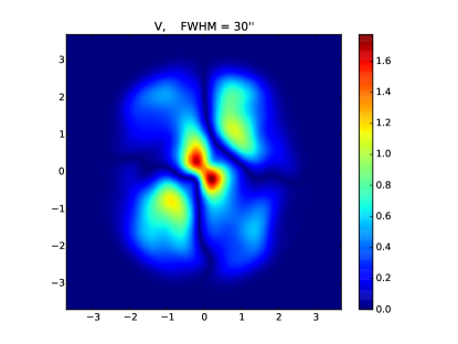
Figure 1: Upper panel: simulated map of the surface brightness of the Stoke’s parameter $V$ at 100 MHz, for a PSF with a FWHM$=30\arcsec$, in units of $10^{28}$ erg s^-1 Hz^-1 str^-1. Lower panel: circular polarized fraction $V/I$ at 100 MHz for the same PSF. Only the region with $I>0.05I_{\rm max}$ is shown. Axes are in primes, centered on the pulsar.

In Fig. 1 we show a map of the Stoke’s parameter $V$ and of the CP fraction computed from our 3D simulation, and convolved with a PSF of $30\arcsec$ FWHM. Maps are shown over the region of the nebula where the intensity is at least 5% of the maximum ($I<0.05I_{\rm max}$), again in order to avoid contaminations from the faint edges. Note that $V$ and the CP fraction scale as a function of the average field strength and observational frequency as: $(\langle B\rangle/100\;\mu{\rm G})^{1/2}(\nu/100{\rm\;MHz})^{-1/2}$, where the average field is defined as the square root of the ratio of total magnetic energy (ordered large scale field plus disordered one) over the nebular volume $\langle B\rangle=\sqrt{8\pi(E_{\rm turb}+E_{\rm ord})/V_{\rm pwn}}$. The CP fraction at this resolution is found to be $V/I\simeq 8.5\times 10^{-4}$, with local maxima $V/I\simeq 2\times 10^{-3}$, located however toward the faint edges of the nebula. A more conservative estimate in the central brighter part within $1^{\prime}$ from the pulsar is $V/I\simeq 5\times 10^{-4}$. Even in the central part of the PWN, as expected from synchrotron theory, the CP fraction is higher where the intensity tends to be smaller, and there are large portions of the nebula where the CP fraction is below $\simeq 5\times 10^{-4}$. In Fig.2 we show how results change with resolution both for the integrated CP fraction and the peak CP fraction. Results clearly show that below a resolution of $\sim 2^{\prime}$, the integrated CP fraction is halved with respect to the value corresponding to the result of Fig. 1. However the numbers are dominated by the edges. The high CP fraction central peaks within $1^{\prime}$ from the pulsar, seen in Fig. 1, with CP fraction $V/I\simeq 0.0015$, disappear already at a resolution of $60\arcsec$.

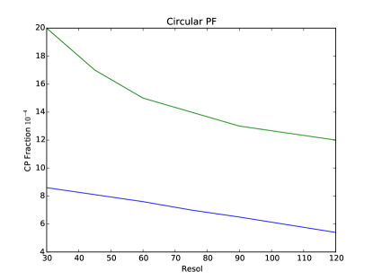
Figure 2: Peak circular polarized fraction (upper green curve) and average circular polarized fraction (lower blue curve), at 100 MHz, from simulated maps, as a function of instrumental resolution given as the full width half maximum of the PSF in arcsec

Stoke’s $V$ can also be generated by Faraday conversion ($I\rightarrow V$, and $Q\rightarrow V$), either inside or outside the source. Concerning the internal Faraday conversion, given that radio emission extends as a power-law to the ionospheric cutoff $\sim 30$ MHZ, one can safely assume a minimal Lorentz factor $\gamma_{\rm min}\mbox{{\raisebox{-1.72218pt}{$\stackrel{{\scriptstyle<}}{{{\scriptstyle\sim}}}$}}}100$ and use the standard analytic formulae by Sazonov (1969) for a power-law distribution (Huang & Shcherbakov, 2011). We found that the induced circular polarization is a few orders of magnitude smaller than the intrinsic one. For Faraday conversion in the ISM we took an electron density $n_{e}=0.015$ cm^-3 and typical average magnetic field $B_{\rm ISM}\approx 1\;\mu$G derived from radio dispersion and rotation measure for the Crab pulsar and nebula (Davidson & Terzian, 1969; Manchester, 1971; Bietenholz & Kronberg, 1991). Taking a typical temperature in the range $10^{4}-10^{5}$K, the induced CP is again found to be several orders of magnitude smaller than the intrinsic one. This implies that the computed CP maps are unaffected by propagation, and that any detection of CP is likely to be intrinsic.

4 Conclusions

In this work, for the first time, we computed the expected circular polarization from synchrotron emission in the Crab nebula, considering that the emitting plasma is mainly composed by electrons and protons, using a state of the art 3D model for the magnetic field geometry inside the PWN. Our results clearly show that previous non detections were not constraining. The upper limit by Wilson & Weiler (1997), obtained at a resolution of $50"\times 150"$ FWHM, would correspond to an integrated CP fraction at 100 MHz of about $7\times 10^{-4}$, which is just at the limit predicted in Fig. 2, and a factor 2 above it if one considers just the brightest part of the nebula. Even the expected peak values at that resolution is estimated to be just a factor 2 above their detection limit. However, as discussed previously, this is mostly due to faint edges. The ability to identify possible peaks strongly relies on resolution: we estimate that a PSF with a FWHM not greater than $60\arcsec$ is required in order to see the brightest inner peaks.

The Crab nebula is a bright object, and the intensity of the Stoke’s parameter $V$ is high enough that it could be easily detected above noise, even with short term observations, by essentially all current radio telescopes. Unfortunately the major issue in polarization measures comes from calibration (Hales, 2017). Calibration leakage among the various Stoke’s parameters and the lack of absolute calibrators set in general limit on the CP detection with $V/I$ at best at the level of few $10^{-3}-10^{-2}$ (Tasse et al., 2013; Perley & Butler, 2013; Murgia et al., 2016; Sokolowski et al., 2017). Rayner, Norris & Sault (2000) have shown that using specifically designed calibration strategies it is possible to get reliable measures up to $V/I\sim 2\times 10^{-3}$ at a few GHz (see also Wiesemeyer et al., 2011), with a typical errors $\sim$ a few $10^{-4}$, and resolution high enough to resolve the Crab nebula inner structures. This is however again at the limit of our predicted values, once scaled to few GHz. Being the Crab nebula a strongly linearly polarized source, it is not even clear if systems with linear polarized feeds improve on circular ones. Part of the problem stems from the fact that there are few circularly polarized targets, and CP science is not a strong driver in the construction of radio facilities, even if there has been an increasing interest in CP (Perley & Butler, 2013; Enßlin et al., 2017; Mao & Wang, 2017).

If special attention is devoted to construction and calibration of the next generation radio telescopes, especially at the low frequency range, it will be feasible to reach the detection limit for the Crab nebula in the forthcoming future.

References

- Abdo et al. (2010) Abdo A. A. et al., 2010, ApJ, 708, 1254
- Achterberg et al. (2001) Achterberg A., Gallant Y. A., Kirk J. G., Guthmann A. W., 2001, MNRAS, 328, 393
- Adriani et al. (2009) Adriani O. et al., 2009, Nature, 458, 607
- Adriani et al. (2013) —, 2013, Soviet Journal of Experimental and Theoretical Physics Letters, 96, 621
- Aguilar et al. (2013) Aguilar M. et al., 2013, Physical Review Letters, 110, 141102
- Aharonian et al. (2004) Aharonian F. et al., 2004, ApJ, 614, 897
- Albert et al. (2008) Albert J. et al., 2008, ApJ, 674, 1037
- Arons (2012) Arons J., 2012, Space Sci. Rev., 173, 341
- Atoyan (1999) Atoyan A. M., 1999, A&A, 346, L49
- Aumont et al. (2010) Aumont J. et al., 2010, A&A, 514, A70
- Baars (1972) Baars J. W. M., 1972, A&A, 17, 172
- Baldwin (1971) Baldwin J. E., 1971, in IAU Symposium, Vol. 46, The Crab Nebula, R. D. Davies & F. Graham-Smith, ed., pp. 22–+
- Bandiera, Neri & Cesaroni (2002) Bandiera R., Neri R., Cesaroni R., 2002, A&A, 386, 1044
- Bandiera & Petruk (2016) Bandiera R., Petruk O., 2016, MNRAS, 459, 178
- Begelman & Li (1992) Begelman M. C., Li Z.-Y., 1992, ApJ, 397, 187
- Bietenholz et al. (1997) Bietenholz M. F., Kassim N., Frail D. A., Perley R. A., Erickson W. C., Hajian A. R., 1997, ApJ, 490, 291
- Bietenholz & Kronberg (1991) Bietenholz M. F., Kronberg P. P., 1991, ApJ, 368, 231
- Blasi & Amato (2011) Blasi P., Amato E., 2011, Astrophysics and Space Science Proceedings, 21, 624
- Blondin, Chevalier & Frierson (2001) Blondin J. M., Chevalier R. A., Frierson D. M., 2001, ApJ, 563, 806
- Bogovalov et al. (2005) Bogovalov S. V., Chechetkin V. M., Koldoba A. V., Ustyugova G. V., 2005, MNRAS, 358, 705
- Bucciantini (2017) Bucciantini N., 2017, MNRAS, 471, 4885
- Bucciantini, Arons & Amato (2011) Bucciantini N., Arons J., Amato E., 2011, MNRAS, 410, 381
- Bucciantini et al. (2017) Bucciantini N., Bandiera R., Olmi B., Del Zanna L., 2017, MNRAS, 470, 4066
- Bucciantini et al. (2003) Bucciantini N., Blondin J. M., Del Zanna L., Amato E., 2003, A&A, 405, 617
- Bucciantini et al. (2005) Bucciantini N., del Zanna L., Amato E., Volpi D., 2005, A&A, 443, 519
- Burch (1979) Burch S. F., 1979, MNRAS, 186, 519
- Davidson & Terzian (1969) Davidson K., Terzian Y., 1969, AJ, 74, 849
- Del Zanna, Amato & Bucciantini (2004) Del Zanna L., Amato E., Bucciantini N., 2004, A&A, 421, 1063
- Del Zanna et al. (2006) Del Zanna L., Volpi D., Amato E., Bucciantini N., 2006, A&A, 453, 621
- Enßlin et al. (2017) Enßlin T. A., Hutschenreuter S., Vacca V., Oppermann N., 2017, Phys. Rev. D, 96, 043021
- Gaensler & Slane (2006) Gaensler B. M., Slane P. O., 2006, ARA&A, 44, 17
- Gallant et al. (1992) Gallant Y. A., Hoshino M., Langdon A. B., Arons J., Max C. E., 1992, ApJ, 391, 73
- Gelfand, Slane & Zhang (2009) Gelfand J. D., Slane P. O., Zhang W., 2009, ApJ, 703, 2051
- Ghisellini et al. (1992) Ghisellini G., Celotti A., George I. M., Fabian A. C., 1992, MNRAS, 258, 776
- Hales (2017) Hales C. A., 2017, AJ, 154, 54
- Hennessy et al. (1992) Hennessy G. S. et al., 1992, ApJLett, 395, L13
- Hester (2008) Hester J. J., 2008, ARA&A, 46, 127
- Hibschman & Arons (2001) Hibschman J. A., Arons J., 2001, ApJ, 560, 871
- Hirotani et al. (2000) Hirotani K., Iguchi S., Kimura M., Wajima K., 2000, ApJ, 545, 100
- Hooper, Blasi & Dario Serpico (2009) Hooper D., Blasi P., Dario Serpico P., 2009, JCAP, 1, 025
- Huang & Shcherbakov (2011) Huang L., Shcherbakov R. V., 2011, MNRAS, 416, 2574
- Kennel & Coroniti (1984a) Kennel C. F., Coroniti F. V., 1984a, ApJ, 283, 694
- Kennel & Coroniti (1984b) —, 1984b, ApJ, 283, 710
- Kino, Kawakatu & Takahara (2012) Kino M., Kawakatu N., Takahara F., 2012, ApJ, 751, 101
- Komissarov (2013) Komissarov S. S., 2013, MNRAS, 428, 2459
- Komissarov & Lyubarsky (2004) Komissarov S. S., Lyubarsky Y. E., 2004, MNRAS, 349, 779
- Kuiper et al. (2001) Kuiper L., Hermsen W., Cusumano G., Diehl R., Schönfelder V., Strong A., Bennett K., McConnell M. L., 2001, A&A, 378, 918
- Legg & Westfold (1968) Legg M. P. C., Westfold K. C., 1968, ApJ, 154, 499
- Linden (2015) Linden T., 2015, ApJ, 799, 200
- Lyne, Pritchard & Graham-Smith (1993) Lyne A. G., Pritchard R. S., Graham-Smith F., 1993, MNRAS, 265, 1003
- Lyutikov (2003) Lyutikov M., 2003, MNRAS, 339, 623
- MacAlpine & Satterfield (2008) MacAlpine G. M., Satterfield T. J., 2008, AJ, 136, 2152
- MacFadyen & Woosley (1999) MacFadyen A. I., Woosley S. E., 1999, ApJ, 524, 262
- Manchester (1971) Manchester R. N., 1971, in IAU Symposium, Vol. 46, The Crab Nebula, Davies R. D., Graham-Smith F., eds., p. 118
- Mao & Wang (2017) Mao J., Wang J., 2017, ApJ, 838, 78
- Martín, Torres & Rea (2012) Martín J., Torres D. F., Rea N., 2012, MNRAS, 427, 415
- McKinney (2005) McKinney J. C., 2005, ApJLett, 630, L5
- Metzger et al. (2011) Metzger B. D., Giannios D., Thompson T. A., Bucciantini N., Quataert E., 2011, MNRAS, 413, 2031
- Mezger et al. (1986) Mezger P. G., Tuffs R. J., Chini R., Kreysa E., Gemuend H.-P., 1986, A&A, 167, 145
- Murgia et al. (2016) Murgia M. et al., 2016, MNRAS, 461, 3516
- Olmi et al. (2013) Olmi B., Del Zanna L., Amato E., Bandiera R., Bucciantini N., 2013, ArXiv e-prints
- Olmi et al. (2014) —, 2014, MNRAS, 438, 1518
- Olmi et al. (2015) Olmi B., Del Zanna L., Amato E., Bucciantini N., 2015, MNRAS, 449, 3149
- Olmi et al. (2016) Olmi B., Del Zanna L., Amato E., Bucciantini N., Mignone A., 2016, Journal of Plasma Physics, 82, 635820601
- Pacini & Salvati (1973) Pacini F., Salvati M., 1973, ApJ, 186, 249
- Perley & Butler (2013) Perley R. A., Butler B. J., 2013, ApJS, 206, 16
- Popham, Woosley & Fryer (1999) Popham R., Woosley S. E., Fryer C., 1999, ApJ, 518, 356
- Porth, Komissarov & Keppens (2014) Porth O., Komissarov S. S., Keppens R., 2014, MNRAS, 438, 278
- Rayner, Norris & Sault (2000) Rayner D. P., Norris R. P., Sault R. J., 2000, MNRAS, 319, 484
- Reynolds et al. (1996) Reynolds C. S., Fabian A. C., Celotti A., Rees M. J., 1996, MNRAS, 283, 873
- Sazonov (1969) Sazonov V. N., 1969, Soviet Ast., 13, 396
- Sironi & Spitkovsky (2011) Sironi L., Spitkovsky A., 2011, ApJ, 741, 39
- Sokolowski et al. (2017) Sokolowski M. et al., 2017, ArXiv e-prints
- Spitkovsky (2006) Spitkovsky A., 2006, ApJLett, 648, L51
- Takata, Ng & Cheng (2016) Takata J., Ng C. W., Cheng K. S., 2016, MNRAS, 455, 4249
- Takata, Wang & Cheng (2010) Takata J., Wang Y., Cheng K. S., 2010, ApJ, 715, 1318
- Tanaka & Asano (2017) Tanaka S. J., Asano K., 2017, ApJ, 841, 78
- Tasse et al. (2013) Tasse C., van der Tol S., van Zwieten J., van Diepen G., Bhatnagar S., 2013, A&A, 553, A105
- Timokhin & Arons (2013) Timokhin A. N., Arons J., 2013, MNRAS, 429, 20
- van der Swaluw et al. (2001) van der Swaluw E., Achterberg A., Gallant Y. A., Tóth G., 2001, A&A, 380, 309
- Veron-Cetty & Woltjer (1993) Veron-Cetty M. P., Woltjer L., 1993, A&A, 270, 370
- Volpi et al. (2008a) Volpi D., Del Zanna L., Amato E., Bucciantini N., 2008a, A&A, 485, 337
- Volpi et al. (2008b) —, 2008b, in American Institute of Physics Conference Series, Vol. 983, 40 Years of Pulsars: Millisecond Pulsars, Magnetars and More, C. Bassa, Z. Wang, A. Cumming, & V. M. Kaspi, ed., pp. 216–218
- Wang, Pun & Cheng (2006) Wang W., Pun C. S. J., Cheng K. S., 2006, A&A, 446, 943
- Weisskopf et al. (2000) Weisskopf M. C. et al., 2000, ApJLett, 536, L81
- Wiesemeyer et al. (2011) Wiesemeyer H., Thum C., Morris D., Aumont J., Rosset C., 2011, A&A, 528, A11
- Wilson & Weiler (1997) Wilson A. S., Weiler K. W., 1997, ApJ, 475, 661
- Wright & Forster (1980) Wright M. C. H., Forster J. R., 1980, ApJ, 239, 873
- Zhdankin et al. (2017) Zhdankin V., Werner G. R., Uzdensky D. A., Begelman M. C., 2017, Physical Review Letters, 118, 055103
- Zrake (2016) Zrake J., 2016, ApJ, 823, 39