Monitoring squeezed collective modes of a 1D Bose gas after an interaction quench using density ripples analysis

Abstract

We investigate the out-of-equilibrium dynamics following a sudden quench of the interaction strength, in a one-dimensional quasi-condensate trapped at the surface of an atom chip. Within a linearized approximation, the system is described by independent collective modes and the quench squeezes the phase space distribution of each mode, leading to a subsequent breathing of each quadrature. We show that the collective modes are resolved by the power spectrum of density ripples which appear after a short time of flight. This allows us to experimentally probe the expected breathing phenomenon. Our results are in good agreement with theoretical predictions which take the longitudinal harmonic confinement into account.

I Introduction

The out-of-equilibrium dynamics of isolated quantum many-body systems is a field attracting a lot of interest polkovnikov_colloquium:_2011 , triggered in part by progress in cold atom experiments. A particular focus has been devoted to the case of sudden quenches where the system is brought out-of-equilibrium by a sudden change of a Hamiltonian parameter, and in particular the case of an interaction quench, both theoretically  and experimentally trotzky_probing_2012 ; cheneau_light-cone-like_2012 ; hung_cosmology_2013 ; langen_double_2017 ; jaskula_acoustic_2012 . Whether and how the system relaxes towards an equilibrium state is the subject of intense theoretical work. The role of integrability, not completely elucidated, is the focus of many studies. Within this context, the case of a 1D Bose gas with contact repulsive interactions, described by the integrable Lieb-Liniger model, is a prime theoretical candidate to uncover the underlying physics, studied in e.g  de_nardis_solution_2014 ; calabrese_interaction_2014 ; cazalilla_quantum_2016 ; swislocki_quantum_2016 .

This paper constitutes the experimental study of the out-of-equilibrium dynamics following a sudden quench of the interaction strength in a 1D Bose gas with repulsive interactions. Within a linearized approximation, the evolution following a splitting of a 1D Bose gas in two copies, studied in langen_double_2017 , can be interpreted as an interaction quench in an effective 1D Bose gas. Investigating the first-order correlation function, the authors observed an apparent thermalization, taking the form of a light cone effect. This observation may however conceal underlying non-equilibrium dynamics, as revealed recently by the observation of recurrences in a similar experiment rauer_recurrences_2017 . Finding appropriate observables revealing these dynamics is thus a key point for investigating out-of-equilibrium phenomena. In this paper, by investigating the density ripples appearing after short time of flight, the behavior of collective modes is probed, rather than a global quantity such as the first-order correlation function, allowing for a better understanding of the physics at play after an interaction quench. The dynamics is revealed by the oscillatory behavior of each component of the density ripples power spectrum, observed for times that go beyond the apparent thermalization time seen on the first order correlation function. We show that these oscillatory dynamics are the signature of squeezed collective modes: for each collective mode, the quench produces a squeezed phase space distribution, leading to a subsequent oscillation of the width of its quadratures — a breathing behavior. As well as improving the understanding of the effect of an interaction quench, this work constitutes an observation of squeezed collective modes, a result interesting on its own.

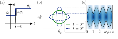
Figure 1: Squeezing of each collective mode after an interaction strength quench from $g_{i}$ to $g_{f}$. The Gaussian phase space distributions before the quench ($t=0^{-}$), just after the quench ($t=0^{+}$) and after an evolution time $\pi/\left(2\omega_{q}\right)$ (dashed ellipse) are represented in (b), where lines correspond to a given probability density (here we chose $\kappa=3$). The subsequent breathing is seen in (c), where the time evolution of the phase distribution is shown in color plot.

II The interaction quench within the linearized approach

The physics at play can be understood by considering a 1D homogeneous Bose gas, of length $L$, temperature $T$ and density $n_{0}$, with particles of mass $m$ interacting with a two-body repulsive contact interaction $g\delta(z)$, where $z$ is the distance between the two particles. At $t=0$, $g$ is suddenly changed from $g_{i}$ to $g_{f}=(1+\kappa)g_{i}$, where $\kappa$ is the quench strength. While the complete treatment of an interaction quench is tremendously difficult the problem is greatly simplified if one can rely on a linearized approach, as presented below. Within the quasi-condensate regime, density fluctuations are strongly reduced ($|\delta{n}(z)|\ll n_{0}$) and phase fluctuations occur on large length scales, such that the Hamiltonian of the system can be diagonalized using the phase-density representation of the field operator $\Psi(z)=\sqrt{n_{0}+\delta{n}(z)}\exp(i{\theta}(z))$ and the Bogoliubov procedure mora_extension_2003 . The obtained linearized modes correspond to Fourier modes. For each wave-vector $q$, the dynamics is governed by the harmonic oscillator Hamiltonian schemmer_monte_2017

$$H_{q}=A_{q}{n}_{q}^{2}+B_{q}{\theta}_{q}^{2}=\hbar\omega_{q}\left({\tilde{n}_{q}^{2}}/{2}+{\tilde{\theta}_{q}^{2}}/{2}\right)$$ (1)

where the canonically conjugated hermitian operators ${n}_{q}$ and ${\theta}_{q}$ are the Fourier components  of $\delta n$ and $\theta$ and where the reduced variables are defined by $\tilde{n}_{q}=n_{q}(A_{q}/B_{q})^{1/4}$ and $\tilde{\theta}_{q}=\theta_{q}(B_{q}/A_{q})^{1/4}$. For wavevectors $q$ much smaller than the inverse healing length $\xi^{-1}=\sqrt{mgn_{0}}/\hbar$, the excitations are of hydrodynamic nature . Their frequency is $\omega_{q}=cq$, where the speed of sound is $c=\sqrt{n_{0}\partial_{n}\mu/m}$, and the Hamiltonian’s coefficients are $B_{q}=\hbar^{2}q^{2}n_{0}/(2m)$ and $A_{q}=mc^{2}/(2n_{0})$. Here $\mu(n)$ is the equation of state of the gas relating the chemical potential $\mu$ to the linear density, which reduces to $\mu=gn$ for pure 1D quasi-condensate. For a given $q$, the dynamics of the quenched harmonic oscillator is represented in Fig. (1). Before the quench the phase space distribution is the one of a thermal state: an isotropic Gaussian in the ($\tilde{\theta}_{q},\tilde{n}_{q}$)-plane. The quench affects $A_{q}$ while $\theta_{q}$ and $n_{q}$ do not have time to change. The variances thus become $\langle\tilde{\theta}_{q}^{2}\rangle_{t=0^{+}}=\langle\tilde{\theta}_{q}^{2}\rangle_{t=0^{-}}/(1+\kappa)^{1/2}$ and $\langle\tilde{\delta n_{q}}^{2}\rangle_{t=0^{+}}=\langle\tilde{\delta n_{q}}^{2}\rangle_{t=0^{-}}(1+\kappa)^{1/2}$. The subsequent evolution is a rotation in phase space at a frequency $\omega_{q}$ leading to a breathing of each quadrature. In particular

$$\langle\theta_{q}^{2}\rangle=\langle\theta_{q}^{2}\rangle_{i}(1+\kappa\sin^{2}(cqt)),$$ (2)

where the initial value $\langle\theta_{q}^{2}\rangle_{i}$ is the thermal prediction $\langle\theta_{q}^{2}\rangle=mk_{B}T/(\hbar^{2}n_{0}q^{2})$ .

Probing the non equilibrium dynamics following a quench is not straightforward, especially concerning the choice of the observable. Since density fluctuations are very small within the quasi-condensate regime, it is more advantageous to probe the phase fluctuations . One way is to investigate the one-body correlation function $g_{1}(z)=\langle\hat{\Psi}^{\dagger}(z)\hat{\Psi}(0)\rangle$, which, for $z\gg\xi$ and in the quasi-condensate regime, writes $g_{1}(z)\simeq n_{0}e^{-\langle(\theta(z)-\theta(0))^{2}\rangle/2}$ mora_extension_2003 . However since phase fluctuations are large in a quasi-condensate, the exponential cannot be linearized and $g_{1}(z)$ mixes contributions from all Bogoliubov modes , preventing the observation of the squeezed dynamics. In fact, the linearized model above predicts the light-cone effect on the $g_{1}$ function: $g_{1}(z)$ changes from its initial exponential decay $\exp(-|z|/l_{c}^{i})$, where $l_{c}^{i}=2\hbar^{2}n_{0}/(mk_{B}T)$, to an exponential decay with a new correlation length $l_{c}^{f}=2l_{c}^{i}/(\kappa+2)$ for $z<2ct$. The breathing of each squeezed Bogoliubov mode is not transparent here. Moreover, for times larger than a few $t^{g_{1}}_{\rm th}=l_{c}^{f}/c$, the $g_{1}$ function essentially reaches the form expected for a thermal state at a temperature $T_{f}=T(\kappa+2)/2$, and the ongoing dynamics is hidden. In this paper we use the density ripples analysis to reveal the non equilibrium dynamics of the gas by probing the breathing of each mode.

III Resolving Bogoliubov modes with density ripples

Density ripples appear after switching the interactions off and waiting for a free evolution time $t_{f}$ (time-of-flight), during which phase fluctuations transform into density fluctuations imambekov_density_2009 ; dettmer_observation_2001 ; manz_two-point_2010 ; rauer_cooling_2016 . Consider the power spectrum of density ripples $\langle|\rho(q)|^{2}\rangle$, where $\rho(q)=(1/\sqrt{L})\int dz(\langle n(z,t_{f})-n_{0})e^{iqz}$. Propagating the field operator during the time of flight and assuming translational invariance we obtain 

$$\langle|\rho_{n_{0}}(q)|^{2}\rangle=\int dxe^{-iqx}(f(q,x)-n_{0}^{2}),$$ (3)

where

$$f(q,x)\simeq n_{0}^{2}\langle e^{i\left[\theta(0)-\theta(-\hbar qt_{f}/m)+\theta(x-\hbar qt_{f}/m)-\theta(x)\right]}\rangle,$$ (4)

averages in Eq. (4) are taken before the time of flight. The function $f$ involves only pairs of points separated by $\hbar qt_{f}/m$. For small wave vectors $q\hbar t_{f}/m\ll l_{c}$, the phase difference between those points is small and one can expand the exponential. To lowest order, assuming uncorrelated distributions for each mode $q$ and vanishing mean values, we then find

$$\langle|\rho_{n_{0}}(q)|^{2}\rangle=4n_{0}^{2}\langle\theta_{q}^{2}\rangle\sin^{2}\left({\hbar q^{2}t_{f}}/{(2m)}\right),$$ (5)

showing that, for low lying $q$, the density ripples spectrum directly resolves the phase quadrature $\langle\theta_{q}^{2}\rangle$ of individual Bogoliubov modes . The proportionality between $\langle|\rho_{n_{0}}(q)|^{2}\rangle$ and $\langle\theta_{q}^{2}\rangle$ implies that $\langle|\rho_{n_{0}}(q)|^{2}\rangle$ oscillates according to Eq. (2) when varying the time $t$ after the quench. Density ripples are thus an ideal tool to investigate the quench dynamics. Note that, in the following we are interested, for each wave vector $q$, in the evolution of $\langle|\rho_{n_{0}}(q)|^{2}\rangle$ with the evolution time $t$, such that the proportionality factor $4n_{0}^{2}\sin^{2}\left({\hbar q^{2}t_{f}}/{(2m)}\right)$ is irrelevant for our data analyis.

In typical experiments, atoms are confined by a smooth potential $V(z)$. For weak enough confinement and for wavelengths much smaller than the system’s size, one can however use the above results for homogeneous systems within a local density approximation (LDA) . Then $\tilde{\rho}(q)=\int dz\delta n(z,t_{f})e^{iqz}$ fulfills $\tilde{\rho}(q)\simeq\int dz\langle|\rho_{n_{0}(z)}(q)|^{2}\rangle$ where $n_{0}(z)$ is the density profile, which can itself be evaluated within the LDA using the gas equation of state and the local chemical potential $\mu(z)=\mu_{0}-V(z)$. Injecting Eq. (2) and Eq. (5) into the LDA integral, we find

$$\langle|\tilde{\rho}(q)|^{2}\rangle/\langle|\tilde{\rho}(q)|^{2}\rangle_{i}=1+\kappa{\cal F}(cqt),$$ (6)

where $c$ is the speed of sound after the quench evaluated at the trap center and ${\cal F}$ only depends on the shape of $V(z)$. For a box-like potential, one recovers previous results and ${\cal F}(\tau)=\sin^{2}(\tau)$. The expression of ${\cal F}$ is given in Appendix D in the case of a harmonic potential: The oscillatory behavior is preserved, although the spread in frequencies originating from the inhomogeneity in $n_{0}$ introduces damping, which is a pure dephasing effect.

IV Experimental realization

The experiment uses an atom-chip set up  where ⁸⁷Rb atoms are magnetically confined using current-carrying micro-wires. The transverse confinement, acting in a vertical plane, is provided by three parallel wires carrying AC-current modulated at 400 kHz, which renders the magnetic potential insensitive to wire imperfections and, allows for independent control of the transverse and longitudinal confinements. We perform radio frequency (RF) forced evaporative cooling until we reach the desired temperature. We then increase the RF frequency by 60 kHz, providing a shield for energetic three-body collision residues and wait during 150 ms relaxation time. The clouds contain a few thousand atoms, in a trap with a transverse frequency $\omega_{\perp}/2\pi=$ 1.5  or 3.1 kHz, depending on the data set, and a longitudinal frequency $\omega_{\parallel}/2\pi=$ 8.5 Hz. The samples are quasi-1D, the temperature and chemical potential satisfying $\mu,k_{B}T<\hbar\omega_{\perp}$. The temperature is low enough so that the gas typically lies well within the quasi-condensate regime kheruntsyan_pair_2003 . The equation of state is well described by $\mu=\hbar\omega_{\perp}(\sqrt{1+4na}-1)$, where $a=5.3~{}$nm is the 3D scattering length fuchs_hydrodynamic_2003 . While, for $na\ll 1$, one recovers the pure 1D expression $\mu=gn$, where $g=2\hbar\omega_{\perp}a$, this equation of state takes the broadening of the transverse size at larger $na$ into account. The longitudinal density profile, well described by the LDA, extends over twice the Thomas-Fermi radius $R_{TF}=\sqrt{2\mu_{0}/m}/\omega_{\parallel}$. The speed of sound derived from the equation of state is $c=c_{\rm{1D}}/(1+4na)^{1/4}$ where $c_{\rm{1D}}=\sqrt{2\hbar\omega_{\perp}na/m}$ is the pure 1D expression. For data presented in this paper, $c/c_{\rm{1D}}$ is close to 0.7. Since the effective interaction strength is proportional to $c^{2}$, it is proportional to $\omega_{\perp}$.

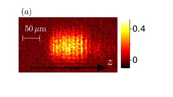
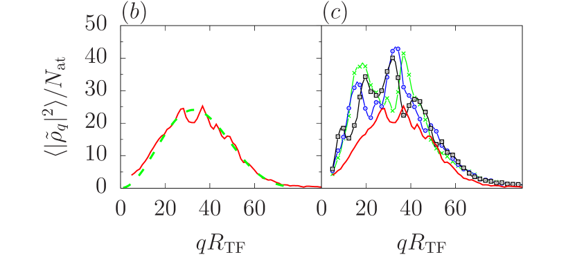
Figure 2: Density ripples analysis (color online). $(a)$ Typical absorption image (optical density shown) taken after a time-of-flight $t_{f}=8~{}$ms. $(b)$ Power spectrum of density ripples, obtained by averaging over about 50 images, for a cloud at thermal equilibrium containing 16000 atoms confined in a trap with frequencies $\omega_{z}/(2\pi)=8.5~{}$Hz and $\omega_{\perp}/(2\pi)=1.5~{}$kHz, yielding a Thomas-Fermi radius $R_{TF}=75~{}\mu$m. The dashed (green) line is a theoretical fit (see text), yielding a temperature $T=55~{}$nK and an optical resolution $\sigma=2.9~{}\mu$m. $(c)$ Power spectra after a quench of strength $\kappa=2$, at times $t=2.1~{}$ms (crosses, green), $t=2.6~{}$ms (circles, blue) and $t=4.6~{}$ms (squares, black), the solid (red) curve being the initial power spectrum.

The interaction strength quench is performed by ramping the transverse trapping frequency $\omega_{\perp}$ from its initial value $\omega_{\perp,i}$ to its final value $\omega_{\perp,f}=(1+\kappa)\omega_{\perp,i}$ within a time $t_{r}$, typically of the order of 1 ms. This time is long enough for the transverse motion of the atoms to follow adiabatically but short enough so that the quench can be considered as almost instantaneous with respect to the probed longitudinal excitations (see Appendix H.1). We simultaneously multiply $\omega_{\parallel}$ by $\sqrt{1+\kappa}$, to avoid modification of the mean profile and of the Bogoliubov wavefunctions(see Appendix E).

In order to probe density ripples, we release the atoms from the trap and let them fall under gravity for a time $t_{f}=8$ ms before taking an absorption image. The transverse expansion, occurring on a time scale of $1/\omega_{\perp}$, ensures the effective instantaneous switching off of the interactions with respect to the probed longitudinal excitations. The density ripples produced by the phase fluctuations present before the free fall are visible in each individual image, as seen in Fig. (2)$(a)$. From the image, we record the longitudinal density profile $\rho(z,t_{f})$ and its discrete Fourier transform  $\tilde{\rho}(q)$. We acquire about 40 images taken in the same conditions with atom number fluctuations smaller than 10%. From this data set, we then extract the power spectrum $\langle|\tilde{\rho}(q)|^{2}\rangle$. We note $\langle|\tilde{\rho}(q)|^{2}\rangle_{i}$ the power spectrum obtained before the quench and a typical spectrum is shown in Fig. (2)$(b)$. We chose to normalize the momenta by $R_{\rm{TF}}^{-1}$: since the Fourier distribution of the $i^{\rm{th}}$ Bogoliubov mode of a 1D quasi-condensate is peaked at $k_{i}\simeq i/R_{TF}$ (see Appendix E), the x-axis roughly corresponds to the mode index. The predicted power spectrum $\langle|\tilde{\rho}(q)|^{2}\rangle_{\rm th}$ is computed using the LDA and analytical solution of Eq. (3) for thermal equilibrium (see Appendices B, C). This expression is peaked around $kR_{\rm{TF}}\simeq\sqrt{\pi m/(\hbar t_{f}})R_{\rm{TF}}\simeq 50$. For comparison with experimental data, we take the imaging resolution into account by multiplying $\langle|\tilde{\rho}(q)|^{2}\rangle_{\rm th}$ with $e^{-q^{2}\sigma^{2}}$ where $\sigma$ is the rms width of the impulse imaging response function, assumed to be Gaussian (Appendix F discusses the effect of this finite optical resolution). The experimental data ultimately compared well with the theoretical predictions, as shown in Fig. (2)$(b)$, where $T$ and $\sigma$ are obtained by fitting the data  . Finally we obtain $k_{B}T/\mu_{0}=0.4$, close to the lowest value obtained in similar setups rauer_cooling_2016 ; jacqmin_sub-poissonian_2011 .

We investigate the dynamics following the quench of the interaction strength by acquiring power spectra of density ripples at different evolution times $t$ after the quench. We typically acquire power spectra every 0.5 ms, over a total time of 5 ms. A few raw spectra are shown in Fig. (2)$(b)$, for a quench strength $\kappa=2.0$. At first sight the power spectra seem erratic. In order to reveal the expected oscillatory behavior of each Fourier component we introduce, for each wavevector $q$ of the discrete Fourier transform, and each measurement time $t$, the reduced time $\tau=cqt$, where $c$ is evaluated for the central density, and compute $J(q,\tau)=\langle|\tilde{\rho}(q)|^{2}\rangle(t)/\langle|\tilde{\rho}(q)|^{2}\rangle_{i}$. We restrict the range of $q$ values to $10<qR_{TF}<40$, to ensure both the condition $q\hbar t_{f}/m\ll l_{c}$ and the validity of the LDA. On the resulting set of spare data, shown in the inset of Fig. (3), an oscillatory behavior appears, despite noise on the data. To combine all the data in a single graph, we perform a “smooth” binning in $\tau$, i.e. we compute, for any given reduced time $\tau$, the weighted averaged of the data with a Gaussian weight function in $\tau$ of width $\Delta=0.31$ : namely we compute $\bar{J}(\tau)=\sum_{\alpha}{J}(q_{\alpha},\tau_{\alpha})e^{-(\tau_{\alpha}-\tau)^{2}/(2\Delta^{2})}/\sum_{\alpha}e^{-(\tau_{\alpha}-\tau)^{2}/(2\Delta^{2})}$, where the sum is done on the data set. The function $\bar{J}(\tau)$, shown in Fig. (3) shows a clear oscillatory behavior.

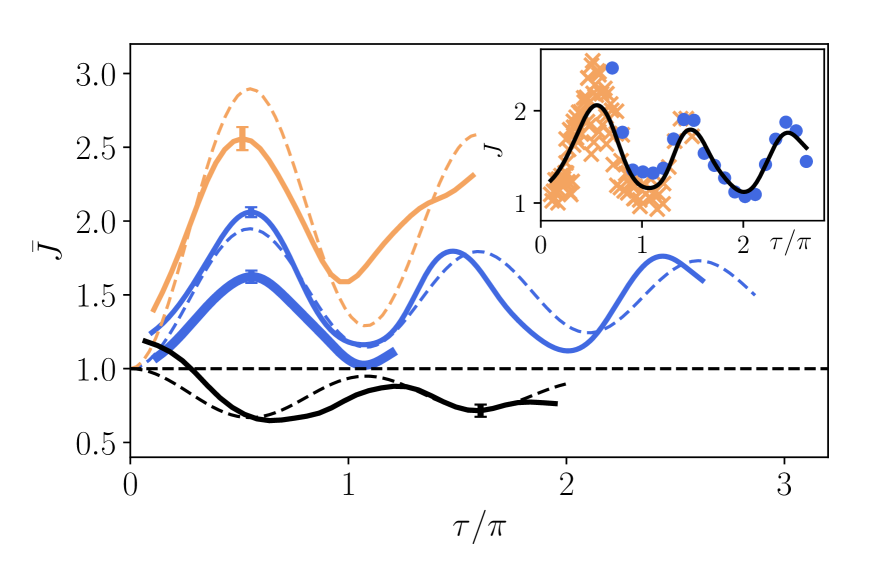
Figure 3: Time evolution of squeezed collective modes produced by an interaction quench. The normalized density ripples power spectrum is plotted versus the reduced time $\tau=cqt$, where the speed of sound $c$ is calculated for the central density. Inset shows the data corresponding to each measurement time and discrete $q$ values, for a data set corresponding to $\kappa=2$ and $\omega_{\perp,i}=2\pi\times 1.5$ kHz, together with the resulting continuous averaged quantity $\bar{J}$ (see text). Orange crosses correspond to $t<t^{g_{1}}_{\rm th}$ and blue circles to $t>t^{g_{1}}_{\rm th}$. The main graph shows the evolution of the experimental smoothed quantity $\bar{J}$ for different data sets. The error bars show the typical statistical uncertainty on $\bar{J}$. The initial transverse oscillation frequency is 1.5 kHz, except for the thick dark grey (blue) curve for which it is 3 kHz. Quench strengths are $\kappa=4$ (light gray (orange)), $\kappa=2$ (dark gray (blue)) data and $\kappa=-0.7$ (black). Dashed lines are theoretical predictions for quench strengths $\kappa=2$ (lightgray (orange)), 1 (light gray) and -0.35 (black).

We repeat the experiment for different quench strengths $\kappa=(\omega_{\perp,f}/\omega_{\perp,i}-1)=\{0.3,3,5\}$, and initial trapping oscillation frequencies $\omega_{\perp}=\{3,1.5\}~{}$kHz. The oscillatory behavior is present in all cases as shown in Fig. (3). We compared the observed oscillations with the theoretical predictions from the linearized model, Eq. (6). The temporal behavior of the data is in good agreement with the predicted one: both the frequency and the observed damping are in agreement with the predictions. The amplitude of the experimental oscillations on the other hand are significantly smaller than the predictions, and in Fig. (3) we plot the theoretical predictions for quench strengths twice as small as the experimental ones. Moreover, for a given quench strength, the observed amplitude depend on the initial transverse frequency, in contradiction with the theoretical model. Several effects leading to a decrease of the oscillation amplitude are discussed in Appendix H. However, they only partially account for the observed amplitude reduction.

V Discussion

In conclusion, analyzing density ripples, we revealed the physics at play after a sudden quench of the interaction strength in a quasi-1D Bose gas, namely the breathing associated to the squeezing of each collective mode. The observed out-of-equilibrium dynamics continues for times larger than $t^{g_{1}}_{\rm th}$, for which the $g_{1}$ function essentially reached its asymptotic thermal behavior  This can be seen in the inset of Fig. (3) where data corresponding to $t>t^{g_{1}}_{\rm th}$, shown in blue circles, still present an oscillatory behavior. This clearly underlines the power of the density ripple analysis to unveil out-of-equilibrium physics. The observed damping is compatible with the sole dephasing effect due to the longitudinal harmonic confinement. At later times, the discreteness of the spectrum and its almost constant level spacing is expected to produce a revival phenomenon. Its observation might however be hindered by a damping of each collective mode due to non-linear couplings. Such a damping occurs, despite the integrability of the 1D Bose gas with contact repulsive interactions, because the Bogoliubov collective modes do not correspond to the conserved quantities. A long-lived non-thermal nature of the state produced by the interaction strength might be revealed either by observing excitations in both the phononic regime and the particle regime of the Bogoliubov spectrum johnson_long-lived_2017 , or, ideally, in finding a way to access the distribution of the Bethe-Ansatz rapidities.

Appendix

This appendix gives technical information and details of calculations. In Appendix A we give a general derivation of the density ripples power spectrum, which does not a priori assume a homogeneous system. Appendix B gives the result for a homogeneous system and the analytical prediction for thermal equilibrium . Appendix C details the derivation of the density ripple power spectrum for a trapped gas, computed using the results for homogeneous gases and the local density approximation. Appendix D provides the explicit calculation of the post-quench evolution of the power spectrum for a harmonically trapped gas, namely the calculation of the function ${\cal F}$ of the main text. In Appendix E we verify the validity of the local density approximation for the parameters of the data presented in the main text. For this purpose, we compute the density ripple power spectrum using the Bogoliubov modes of the trapped gas. In Appendix F, we investigate the effect of finite resolution on the measured density ripple power spectrum. We also make the link between the power spectrum and the auto-correlation function, which permits to compare our data at thermal equilibrium with previously published work. In Appendix G, we justify that interactions play a negligible role during time-of-flight, so that the calculations of the density ripples power spectrum, which assume instantaneous switch-off of the interactions, are valid. In Appendix H, we investigate two effects responsible for a reduction of the oscillation amplitude of the quantity $\bar{J}(\tau)$, extracted from the data, as compared to the simple theoretical predictions Eq. (6) of the main text: First the finite ramp time of the interaction strength decreases the squeezing of the collective modes, and second the finite resolution in $\tau$ resulting from data binning is responsible for a decrease of the expected oscillation amplitude on the processed data.

Appendix A Derivation of the density ripples power spectrum

The power spectrum of density ripples has been first investigated in the limit of small density ripples and for a gas initially in the 3D Thomas-Fermi regime (i.e. $\mu\gg\hbar\omega_{\perp}$) dettmer_observation_2001 ; hellweg_phase_2001 . It was then computed assuming instantaneous switching off of the interactions in imambekov_density_2009 . Here, for consistency, we rederive Eq. (4) and (5) of the main text. Since we will later consider trapped gases, let us first assume a general scenario where we do not restrict ourselves to the homogeneous case. We let the gas evolve freely for a time $t_{f}$ after interactions have been switched off. The power spectrum of the density fluctuations after $t_{f}$ writes

$$\langle|\tilde{\rho}(q)|^{2}\rangle=\int\int dz_{1}dz_{2}e^{iq(z_{1}-z_{2})}\langle\delta n(z_{1},t_{f})\delta n(z_{2},t_{f})\rangle.$$ (7)

Writing $\delta n(z)=n(z)-\langle n(z)\rangle$ and expanding the above equation, the term $|\int dze^{iqz}\langle n(z,t_{f})\rangle|^{2}$ appears. Here we consider times of flight short enough so that the shape of the cloud barely changes during time of flight, so that $\langle n(z,t_{f})\rangle\simeq\langle n(z,0)\rangle$. We moreover consider wavevectors $q$ much larger than the inverse of the cloud length, such that $|\int dze^{iqz}\langle n(z,0)\rangle|^{2}$ is a negligible quantity. We then have

$$\langle|\tilde{\rho}(q)|^{2}\rangle\simeq\int\int dz_{1}dz_{2}e^{iq(z_{1}-z_{2})}\langle n(z_{1},t_{f})n(z_{2},t_{f})\rangle.$$ (8)

To compute $n(z,t_{f})=\Psi^{+}(z,t_{f})\Psi(z,t_{f})$ we evolve the atomic field with the free-particle propagator, which leads to

$$\psi(z,t_{f})=\frac{1}{\sqrt{2\pi t_{f}}}\int d\alpha\psi(\alpha,0)e^{i\frac{(z-\alpha)^{2}}{2t_{f}}},$$ (9)

where for simplicity we use a unit system in which $m=\hbar=1$. We then have

$$\langle n(z_{1},t_{f})n(z_{2},t_{f})\rangle=\frac{1}{(2\pi t_{f})^{2}}\int\int\int\int d\alpha d\beta d\gamma d\delta\langle\psi^{+}_{\alpha}\psi_{\beta}\psi^{+}_{\gamma}\psi_{\delta}\rangle e^{-i\frac{(z_{1}-\alpha)^{2}}{2t_{f}}}e^{i\frac{(z_{1}-\beta)^{2}}{2t_{f}}}e^{-i\frac{(z_{2}-{\gamma})^{2}}{2t_{f}}}e^{i\frac{(z_{2}-\delta)^{2}}{2t_{f}}},$$ (10)

where we use the simplified notation $\psi_{\nu}=\psi(\nu,0)$. Expanding the exponentials, the above expression writes

$$\langle n(z_{1},t_{f})n(z_{2},t_{f})\rangle=\frac{1}{(2\pi t_{f})^{2}}\int\int\int\int d\alpha d\beta d\gamma d\delta\langle\psi^{+}_{\alpha}\psi_{\beta}\psi^{+}_{\gamma}\psi_{\delta}\rangle e^{i\frac{(\alpha-\beta)z_{1}}{t_{f}}}e^{i\frac{\beta^{2}-\alpha^{2}}{2t_{f}}}e^{i\frac{(\gamma-\delta)z_{2}}{t_{f}}}e^{i\frac{\delta^{2}-\gamma^{2}}{2t_{f}}}.$$ (11)

Injecting into Eq. (8), and using $\int dze^{ikz}=2\pi\delta(k)$ and $\delta(x/\alpha)=\alpha\delta(x)$, we get

$$\langle|\tilde{\rho}(q)|^{2}\rangle=\int\int d\alpha d\delta\langle\psi^{+}_{\alpha}\psi_{\alpha+qt_{f}}\psi^{+}_{\delta+qt_{f}}\psi_{\delta}\rangle e^{-i\frac{\alpha^{2}}{2t_{f}}}e^{i\frac{(\alpha+qt)^{2}}{2t_{f}}}e^{-i\frac{(\delta+qt)^{2}}{2t_{f}}}e^{i\frac{\delta^{2}}{2t_{f}}}.$$ (12)

Defining $\delta=\alpha+X$, we obtain

$$\langle|\tilde{\rho}(q)|^{2}\rangle=\int\int d\alpha dXe^{iqX}\langle\psi^{+}_{\alpha}\psi_{\alpha+qt_{f}}\psi^{+}_{\alpha+X+qt_{f}}\psi_{\alpha+X}\rangle.$$ (13)

For gases lying deep in the quasi-condensate regime, one can neglect density fluctuations when estimating the expectation value in the above equation, such that

$$\langle|\tilde{\rho}(q)|^{2}\rangle\simeq\int\int d\alpha dXe^{iqX}\sqrt{n(\alpha)n(\alpha+qt_{f})n(\alpha+X+qt_{f})n(\alpha+X)}\langle e^{i(\theta(\alpha)-\theta({\alpha+qt_{f}})+\theta({\alpha+X+qt_{f}})-\theta({\alpha+X}))}\rangle.$$ (14)

The following section applies this result to homogeneous systems. This equation is however not restricted to homogeneous systems and we will use it to treat the effect of the trap beyond the local density approximation.

Appendix B Power spectrum of the density ripples for a homogeneous gas

For a homogeneous gas, the relevant quantity is an intensive variable which relates to the expression $\langle|\tilde{\rho}(q)|^{2}\rangle$ of the previous section by

$$\langle|\rho(q)|^{2}\rangle=\frac{1}{L}\langle|\tilde{\rho}(q)|^{2}\rangle$$ (15)

where $L$ is the length of the box. Injecting Eq. (14) into Eq. (15), we recover Eq. (3) and (4) of the main text, up to an irrelevant term in $\delta(q)$ . In fact, Wick’s theorem is applicable since $\theta$ is a Gaussian variable , which leads to

$$\frac{\langle|{\rho}(q)|^{2}\rangle}{n_{0}^{2}}=\int dXe^{iqX-\frac{1}{2}\langle(\theta(0)-\theta({qt_{f}})+\theta({X+qt_{f}})-\theta({X}))^{2}\rangle}.$$ (16)

To compute the power spectrum of density ripples for a thermal equilibrium state, we follow the calculation made in imambekov_density_2009 and expand the exponential term in Eq. (16) as a function of the first order correlation function $g^{(1)}(z)=n_{0}e^{-\frac{1}{2}\langle(\theta(0)-\theta(z))^{2}\rangle}$, which fulfils $g^{(1)}(z)=n_{0}e^{-|z|/l_{c}}$ where $l_{c}=2\hbar^{2}n_{0}/(k_{B}T)$ imambekov_density_2009 . Calculation of the integral in Eq. (16) then leads to

$$\frac{\langle|{\rho}(q)|^{2}\rangle}{n_{0}^{2}}=\frac{4ql_{c}}{q(4+l_{c}^{2}q^{2})}\\ -\frac{4e^{-\frac{2\hbar qt_{f}}{ml_{c}}}\left(ql_{c}\cos(\frac{\hbar q^{2}t_{f}}{m})+2\sin(\frac{\hbar q^{2}t_{f}}{m})\right)}{q(4+l_{c}^{2}q^{2})}.$$ (17)

Note that we corrected the formula given in imambekov_density_2009 . The power spectrum computed with this equation is compared in Fig. 4 to the approximated formula valid for small $q$, namely Eq. (5) of the main text.

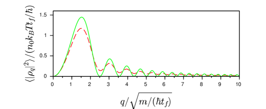
Figure 4: Density ripples power spectrum for a homogeneous gas. The exact formula Eq. (17) (dashed curve) is compared to the small $q$ approximation given Eq. (5) of the main text, where $\langle|{\rho}(q)|^{2}\rangle$ is proportional to $\langle\theta_{q}^{2}\rangle$ (solid curve). The only relevant parameter is $\hbar t_{f}/(ml_{c}^{2})$. Results are shown for $\hbar t_{f}/(ml_{c}^{2})=0.05$, a value corresponding to the data depicted in Fig. (2,b) of the main text, the correlation length $l_{c}=2\hbar^{2}n_{0}/(mk_{B}T)$ being computed for the central density. The effect of the imaging resolution is to multiply this theoretical power spectrum with $e^{-\sigma^{2}q^{2}}$, where $\sigma$ is the rms width of the imaging pulse response function, assumed to be Gaussian. For our data, $\sigma\sqrt{m/(\hbar t_{f})}=0.85$ and only the first maximum of $\langle|{\rho}(q)|^{2}\rangle$ remains visible.

Appendix C Density ripple power spectrum for a harmonically confined gas under the LDA

Let us investigate the density ripples power spectrum in the case of a gas trapped in a longitudinal potential smooth enough so that the cloud size $L$ is much larger than the typical phase correlation length $l_{c}$ and much larger than $\hbar qt_{f}/m$: $L\gg l_{c},\hbar qt_{f}/m$. As in section A, we moreover consider the power spectrum for wavevectors $q\gg 1/L$. Let us start with the general expression Eq. (7) that we write

$$\langle|\tilde{\rho}(q)|^{2}\rangle=\int dz\int du\langle\delta\rho(z,t_{f})\delta\rho(z+u,t_{f})\rangle e^{iqu}.$$ (18)

Consider $\langle\delta\rho(z,t_{f})\delta\rho(z+u,t_{f})\rangle$ for a given $z$. This expression vanishes over a length much smaller than $L$, so values of $u$ significantly contributing to the integral are much smaller than $L$. Moreover the region of the initial cloud contributing most to $\langle\delta\rho(z,t_{f})\delta\rho(z+u,t_{f})\rangle$ is much smaller than $L$ for sufficiently large $L$. Then, to compute $\langle\delta\rho(z,t_{f})\delta\rho(z+u,t_{f})\rangle$ one can perform a local density approximation and use the result of a homogeneous gas at a density $n_{0}(z)$. We then obtain

$$\langle|\tilde{\rho}(q)|^{2}\rangle=\int dz\langle|{\rho}_{n_{0}(z)}(q)|^{2}\rangle$$ (19)

where the subscript $n_{0}(z)$ specifies that one considers the result for a homogeneous gas of density $n_{0}(z)$. This expression is referred to as the local density approximation expression (LDA) of the power spectrum. We have tested this approximation, for conditions close to the experimental data presented in the main text, by comparing it with calculations based on the Bogoliubov excitations of the trapped system (see section E).

Appendix D Time evolution of the density ripple power spectrum for a harmonically confined gas

Here we give an explicit derivation of Eq. (6) of the main text, for a gas harmonically confined in a longitudinal trap of frequency $\omega_{\parallel}$. Injecting Eq. (5) and Eq. (2) of the main text into Eq. (19), and using the local initial power spectrum of $\theta$ which writes $\langle\theta_{q}^{2}\rangle=mk_{B}T/(\hbar^{2}n_{0}q^{2})$, we derive Eq. (6) of the main text with

$${\cal F}=\int dzn_{0}(z)\sin^{2}\left(c(z)qt\right)/N$$ (20)

where $N$ is the total atom number. The density profile $n_{0}(z)$ is estimated itself within the LDA, using the local chemical potential

$$\mu(z)=\mu_{p}(1-(z/R_{\rm{TF}})^{2})),$$ (21)

where $R_{\rm{TF}}$ is the Thomas-Fermi radius of the density profile and $\mu_{p}$ is the chemical potential at the trap center. For a transverse harmonic confinement of frequency $\omega_{\perp}$, it has been checked, by comparing with predictions of the 3D Gross-Pitaevskii equation, that the equation of state of the gas is very well described by the heuristic formula fuchs_hydrodynamic_2003

$$\mu(n)=\hbar\omega_{\perp}\left(\sqrt{1+4na}-1\right),$$ (22)

where $a$ is the 3D scattering length between atoms. For small linear densities, we recover the 1D expression $\mu=2\hbar\omega_{\perp}an$, valid far from the confinement-induced resonance olshanii_atomic_1998 . Using Eq. (22) and Eq. (21), we obtain the density profile

$$n_{0}(z)=\left[\left(\eta(1-\tilde{z}^{2})+1\right)^{2}-1\right]/(4a)$$ (23)

where we introduced $\tilde{z}=z/R_{\rm{TF}}$ and $\eta=\mu_{p}/(\hbar\omega_{\perp})$. This yields $N=(4/3\eta+8\eta^{2}/15)R_{\rm{TF}}/(2a)$. The local speed of sound on the other hand, obtained from the thermodynamic relation $c=\sqrt{n(\partial\mu/\partial n)/m}$, writes

$$c(z)=c_{p}\sqrt{\frac{(1+\eta)\left[\left(1+\eta(1-\tilde{z}^{2})\right)^{2}-1\right]}{\left(1+\eta(1-\tilde{z}^{2})\right)\left((1+\eta)^{2}-1\right)}},$$ (24)

where $c_{p}$ is the speed of sound computed for the central density. Injecting into Eq. (20), we then find

$${\cal F}=\frac{1}{4\eta/3+8\eta^{2}/15}\int_{0}^{1}d{\tilde{z}}\left[\left(1+\eta(1-\tilde{z}^{2})\right)^{2}-1\right]\sin^{2}\left(\tau\sqrt{\frac{(1+\eta)\left[\left(1+\eta(1-\tilde{z}^{2})\right)^{2}-1\right]}{\left(1+\eta(1-\tilde{z}^{2})\right)\left((1+\eta)^{2}-1\right)}}\right).$$ (25)

When the gas is deeply 1D, namely for $\eta\ll 1$, this expression reduces to

$${\cal F}_{\rm{1D}}=\frac{3}{2}\int_{0}^{1}d{\tilde{z}}(1-\tilde{z}^{2})\sin^{2}\left(\tau\sqrt{1-\tilde{z}^{2}}\right).$$ (26)

Experimentally, values of $\eta$ are in the range $[0.6;1.3]$. Fig. 5 shows the function ${\cal F}$, computed for $\eta=1$. We compare it to ${\cal F}_{\rm{1D}}$ and to the expression expected for a homogeneous gas, namely $\sin^{2}(\tau)$.

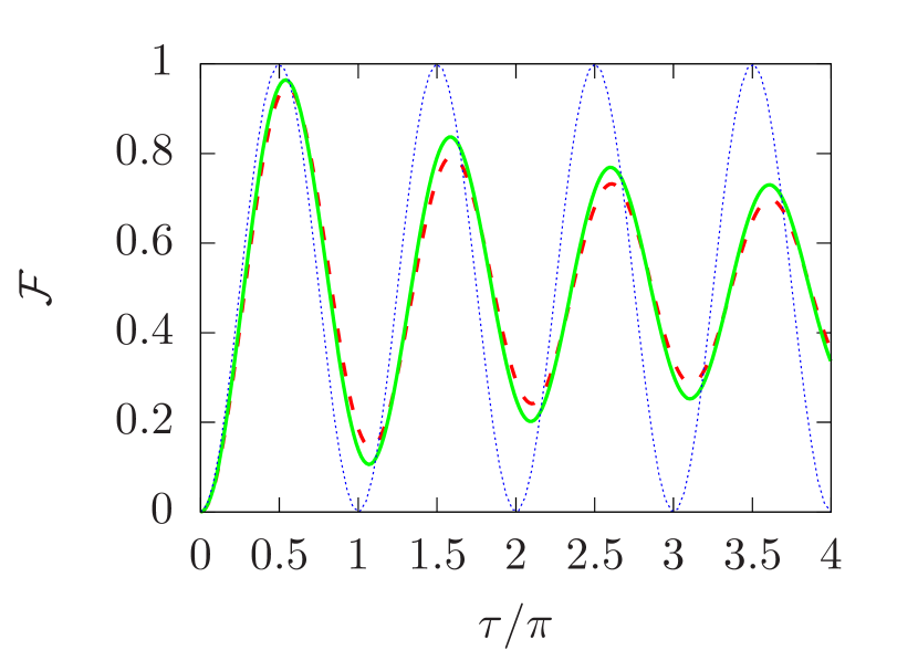
Figure 5: Oscillation of each spectral component of the power spectrum for a harmonically confined gas in the LDA (color online). The function ${\cal F}$ is shown in thick solid lines (green), for $\eta=\mu_{p}/(\hbar\omega_{\perp})=1.0$. The pure 1D limit, corresponding to $\eta\ll 1$ is shown as dashed (red) lines. The undamped oscillations expected for a homogeneous gas are shown in dotted (blue) line. In all the cases, $\tau=cqt$ where $c$ is the central sound velocity.

Appendix E Beyond the LDA: calculation using Bogoliubov modes of a harmonically confined 1D gas

Here we consider a 1D gas confined longitudinally in a harmonic trap of frequency $\omega_{\parallel}$. In opposition to the calculations done in the previous section we do not rely on the local density approximation but use the Bogoliubov modes of the trapped gas to compute the post-quench evolution and the density ripples power spectrum. The relevant collective modes lie deep in the phononic regime. The Bogoliubov modes, indexed by an integer $\nu$, then acquire an analytical dispersion relation and analytical wavefunctions that one can use for calculations. For each mode, the dynamics are accounted for by the harmonic oscillator Hamiltonian

$$H_{\nu}=\hbar\omega_{\nu}\left(\frac{x_{\nu}^{2}}{2}+\frac{p_{\nu}^{2}}{2}\right),$$ (27)

where $\omega_{\nu}=\omega_{\parallel}\sqrt{\nu(\nu+1)/2}$ and $x_{\nu}$ and $p_{\nu}$ are canonically conjugate variables. The phase and density fluctuation operators write

$$\left\{\begin{array}[]{l}\theta(z)=\sum_{\nu}{\theta_{\nu}}(z)p_{\nu}\\ \delta n(z)=\sum_{\nu}{n_{\nu}}(z)x_{\nu}\\ \end{array}\right.$$ (28)

where

$$\left\{\begin{array}[]{l}{\theta_{\nu}}(z)=\frac{1}{\sqrt{2}}\left(\frac{mg}{\hbar^{2}n_{p}}\right)^{1/4}\frac{\sqrt{2\nu+1}}{\left(\nu(\nu+1)\right)^{1/4}}P_{\nu}(\frac{z}{R_{TF}})\\ {n_{\nu}}(z)=\frac{\sqrt{2\nu+1}}{2R_{\rm{TF}}}\left(\nu(\nu+1)\right)^{1/4}\left(\frac{\hbar^{2}n_{p}}{mg}\right)^{1/4}P_{\nu}(\frac{z}{R_{TF}}).\\ \end{array}\right.$$ (29)

Here $n_{p}$ and $R_{TF}$ are the central density and radius of the Thomas-Fermi profile $n_{0}(z)=n_{p}(1-(z/R_{TF})^{2})$ and $P_{\nu}$ are the Legendre polynomials. The interaction quench consists of a sudden change of the interaction parameter $g$ from $g_{i}$ to $g_{f}=(1+\kappa)g_{i}$ at $t=0$, while changing the longitudinal oscillation frequency by a factor $\sqrt{1+\kappa}$ so that $R_{\rm{TF}}$ stays constant. Then the interaction quench preserves the shapes of the wavefunctions $\theta_{\nu}$ and $n_{\nu}$, and it simply changes the canonical variables $x_{\nu}$ and $p_{\nu}$ according to

$$\left\{\begin{array}[]{l}x_{\nu}(t=0^{+})=(g_{f}/g_{i})^{1/4}x_{\nu}(t=0^{-})\\ p_{\nu}(t=0^{+})=(g_{i}/g_{f})^{1/4}p_{\nu}(t=0^{-})\end{array}\right.$$ (30)

Under such a transformation, the initial thermal state, an isotropic Gaussian, becomes a squeezed state and its subsequent evolution under the Hamiltonian Eq. (27) leads to a breathing of each quadrature. In particular

$$\langle p_{\nu}^{2}\rangle=\langle p_{\nu}^{2}\rangle_{i}\left(1+\kappa\sin^{2}(\omega_{\nu}t)\right).$$ (31)

The initial value $\langle p_{\nu}^{2}\rangle_{i}$ is given by the thermal expectation value, which reduces to

$$\langle p_{\nu}^{2}\rangle_{i}=k_{B}T/(\hbar\omega_{\nu})$$ (32)

for the low-lying modes for which $k_{B}T\gg\hbar\omega_{\nu}$.

Injecting Eq. (28) into Eq. (14), using Wick’s theorem and the fact that different modes are uncorrelated we get

$$\langle|\tilde{\rho}(q)|^{2}\rangle=\int\int d\alpha dX\begin{array}[t]{l}e^{iqX}\sqrt{n_{0}(\alpha)n_{0}(\alpha+qt_{f})n_{0}(\alpha+X+qt_{f})n_{0}(\alpha+X)}\\ e^{-\frac{1}{2}\sum_{\nu}\langle p_{\nu}^{2}\rangle\left(\theta_{\nu}(\alpha)-\theta_{\nu}({\alpha+qt_{f}})+\theta_{\nu}({\alpha+X+qt_{f}})-\theta_{\nu}({\alpha+X})\right)^{2}}.\end{array}$$ (33)

For $\hbar qt_{f}/m\ll l_{c}$, where $l_{c}$ is the phase correlation length, one can expand the exponential and $\langle|\tilde{\rho}(q)|^{2}\rangle$ is obtained by summing the contribution of each mode. Since the Legendre polynomials behave as $\cos((\nu+1/2)x+\pi/4)$ at small $x$, the contribution of the mode $\nu$ is peaked at $q\simeq\nu/R_{TF}$.

The predictions of Eq. (33) may be compared to the one obtained within the Local density approximation. Here we focus on the case of thermal equilibrium. We compute the density ripple spectrum injecting the thermal equilibrium value Eq. (32) and the mode wavefunction Eq. (29) into Eq. (33). Fig. 6 shows the result for a cloud whose Thomas-Fermi radius fulfils $l_{c}/R_{\rm{TF}}=0.2$, where $l_{c}=2\hbar^{2}n_{p}/(mk_{B}T)$ is the correlation length of the first order correlation function at the center of the cloud, and for a time-of-flight $t_{f}=6\times 10^{-4}mR_{\rm{TF}}^{2}/\hbar$. These parameters are close to the experimental ones. We compared the results with the LDA, together with the analytical formula for homogeneous gases Eq. (17) and we find excellent agreement. We also compare with the LDA but using, instead of Eq. (17), the approximation Eq. 5 of the main text. We find very good agreement as long as $qR_{\rm{TF}}<50$.

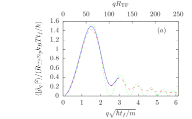
Figure 6: Test of the local density approximation (LDA) (color online). The plot shows the density ripples spectrum of a gas at thermal equilibrium confined in a harmonic potential. The complete calculation, based on the expansion on the Bogoliubov modes, whose wavefunctions are given by the Legendre polynomial, is shown in solid line (blue). It is in excellent agreement with the spectrum computed within the local density approximation (LDA) shown in dashed line (red). The further approximation of small wavevectors, Eq. (5) of the main text, injected into the LDA, shown in dotted line (green), is also in good agreement, for wavevectors fulfilling $qR_{\rm{TF}}<50$. Calculations are done for a Thomas-Fermi radius $l_{c}/R_{\rm{TF}}=0.2$ and and time-of-flight $t_{f}=0.015ml_{c}^{2}/\hbar$, where $l_{c}=2\hbar^{2}n_{p}/(mk_{B}T)$ is the correlation length at the center of the cloud. These parameters are close to those of the experimental data.

Appendix F Effect of a finite optical resolution and auto-correlation function

The effect of the imaging resolution is to multiply the theoretical power spectrum of density ripples with $e^{-\sigma^{2}q^{2}}$, where $\sigma$ is the rms width of the imaging pulse response function, assumed to be Gaussian. The resulting power spectrum, for a harmonically confined cloud at thermal equilibrium, is shown in Fig. (7) for $\sigma\sqrt{m/(\hbar t_{f})}=0.85$, a value typical for our experiments. The large $q$ behavior of the power spectrum is highly dominated by the effect of resolution and only the first maximum of $\langle|{\rho}(q)|^{2}\rangle$ remains visible. Fitting the experimental power spectrums for clouds at thermal equilibrium, we extract both the temperature and the imaging resolution (see Fig. (2) of the main text). The obtained rms widths $\sigma$, close to 3 $\mu$m, are compatible with the expected values if one takes into account the depth of focus of our imaging system ($\simeq 5\mu$m) and the fact that, after the the expansion time $t_{f}$ the cloud explores several tens of $\mu$m along the imaging axis. Note finally that the imaging resolution is irrelevant for the investigation of the dynamics following an interaction quench, since, for each Fourier component $q$, we investigate the time behavior of the normalised quantity $\langle|\tilde{\rho}(q)|^{2}\rangle(t)/\langle|\tilde{\rho}(q)|^{2}\rangle_{i}$ (see main text): the imaging resolution has no effect on this normalised quantity.

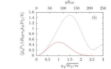
Figure 7: Effect of the finite resolution (color online). We consider a clould at thermal equilibrium in a harmonic potential with the same parameters as in Fig. 6. The power spectrum for infinite resolution (blue dashed curve) is compared to the power spectrum expected for a finite imaging resolution (red solid curve). The effect of the imaging resolution is to multiply the power spectrum with $e^{-\sigma^{2}q^{2}}$, where $\sigma$ is the rms width of the imaging pulse response function, assumed to be Gaussian. Here we took $\sigma\sqrt{m/(\hbar t_{f})}=0.85$, a value close to that of experimental data.

In our paper, we extract from the data the density ripple power spectrum since it is the relevant quantity that enable to resolve the collective Bogoliubov modes. Alternatively, one could consider the auto-correlation function of the density ripples $C(u)=\int dz\langle\delta n(z)\delta n(z+u)\rangle dz$, which is the Fourier transform of the density ripple power spectrum: $C(u)=1/(2\pi)\int dq\langle|\tilde{\rho}(q)|^{2}\rangle e^{-iqu}$. In manz_two-point_2010 , the authors introduced the normalised auto-correlation function $g_{2}(u)=1+C(u)/\int du\langle n(z)\rangle\langle n(z+u)\rangle$. Fig. (8) shows $g_{2}(u)$ for the data at thermal equilibrium (before the quench) shown in Fig. (2) of the main text. A behavior very similar to that observed in manz_two-point_2010 is recovered.

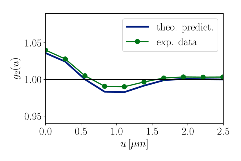
Figure 8: Normalised auto-correlation function of the density ripples. The data set used is the same as that of Fig. (2)(b) of the main text. Experimental data are shown in green and the theoretical prediction for a cloud at a temperature $T=55$ nK and an optical resolution $\sigma=2.9~{}\mu$m is shown in blue.

Appendix G Beyond instantaneous interaction switch off: finite transverse expansion time

In the data presented in the main text, the frequency of the probed longitudinal modes, of the order of $cq$, is no more than $0.15\times\omega_{\perp}$. Then, due to the rapid transverse expansion, interactions during time-of-flight become almost instantaneously negligible and are expected to give only minor corrections to the density ripples spectrum computed for an instantaneous switching off of the interactions. It is nevertheless interesting to estimate their effect. This has already been computed in hellweg_phase_2001 , in the limit $\mu\gg\hbar\omega_{\perp}$ and using time-dependent Bogoliubov equations, i.e. equations of motion linearized in density fluctuations and phase gradient. The linearized calculations a priori require that density fluctuations stay small. Although in our case density ripples at the end of the time-of-flight have large amplitudes, the Bogoliubov calculations hold for the small $q$ components, which fulfil $q\ll ml_{c}/(\hbar t_{f})$ and which are considered in our paper. The condition $\mu\gg\hbar\omega_{\perp}$ on the other hand is not verified for the data shown in the main text. We nevertheless believe that the calculations of hellweg_phase_2001 give a relevant estimation of the effect of interactions during the time-of-flight for our data. From results of hellweg_phase_2001 , we find that the density ripples power spectrum for the small $q$ wavevectors, given by equation (5) of the main text, should be corrected by the factor

$$\mathcal{C}=\left(\omega_{\perp}t_{f}\right)^{-{\left(\frac{cq}{\omega_{\perp}}\right)^{2}}}.$$ (34)

In all experimental situations $\mathcal{C}>0.95$, which confirm that the effect of interactions during the time-of-flight is small.

Appendix H Effects which may reduce the oscillation amplitude

In this section we investigate two effects responsible for a reduction of the amplitude of the oscillations of $\bar{J}$ (see main text), as compared to the theoretical prediction given by Eq. (6) of the main text. We first consider the effect of the finite ramp time of the interaction strength, which reduces the squeezing of the Bogoliubov modes, as compared to an instantaneous quench. This effect contributes to the reduction of the amplitude on the order of 10%. We then investigate the reduction of the amplitude induced by the binning of the data with a finite resolution in $\tau$. This effect amounts to an additional reduction of the amplitude by 18%.

H.1 Beyond the instantaneous quench: finite ramp time

In the experiment, the change of the effective interaction strength is not instantaneous: to ensure the adiabatic following of the transverse motion, we perform a ramp of the transverse oscillation frequency during a time $t_{r}$. The finite value of $t_{r}$ is responsible for a decrease of the induced squeezing of each mode. In the asymptotic limit of very large $t_{r}$, the squeezing vanishes since then, the modes follow adiabatically the modification of the interaction strength. In the following we compute the effect of the ramp on the squeezing of each mode and we use this result to compute the resulting decrease of the oscillation amplitude of $\bar{J}$.

In order to estimate the effect of the finite ramp time, we will consider a homogeneous gas for simplicity. The Bogoliubov modes are then described by the Hamiltonian of Eq. (1) of the main text, namely

$$H_{q}=A_{q}n_{q}^{2}+B_{q}\theta_{q}^{2}.$$ (35)

We regard the effect of a ramp of $\omega_{\perp}$ between the time $t=0$ and the time $t_{r}$: $\omega_{\perp}$ goes from $\omega_{\perp}^{i}$ to $\omega_{\perp}^{f}=(\kappa+1)\omega_{\perp}^{i}$, as depicted in Fig. (9). The coefficient $B_{q}=n_{0}\hbar^{2}q^{2}/(2m)$ is time-independent, while the coefficient $A_{q}$ evolves linearly during the ramp (i.e. during time interval $0<t<t_{r}$), since it is proportional to $c^{2}$, itself proportional to $\omega_{\perp}$. Then, the solution of the second order equations describing the evolution of $\theta_{q}$ and $n_{q}$ during the ramp is given in terms of the Airy functions. In order to investigate the squeezing, it is natural to introduce the reduced variables

$$\left\{\begin{array}[]{l}\tilde{\theta}_{q}=\theta_{q}/\bar{\theta}_{q}\\ \tilde{n}_{q}=n_{q}/\bar{n}_{q}\\ \end{array}\right.$$ (36)

where $\bar{\theta}_{q}=(A_{q}(t)/B_{q})^{1/4}$ and $\bar{n}_{q}=(B_{q}/A_{q}(t))^{1/4}$ are the time-dependent widths of the ground state. For given initial values, the values of $\tilde{\theta}_{q}$ and $\tilde{n}_{q}$ at the end of the ramp are

$$\left(\begin{array}[]{l}\tilde{\theta}_{q}(t_{r})\\ \tilde{n}_{q}(t_{r})\end{array}\right)=M\left(\begin{array}[]{l}\tilde{\theta}_{q}(0)\\ \tilde{n}_{q}(0)\end{array}\right)$$ (37)

where the matrix M has the following components:

$$\left\{\begin{array}[]{l}M_{11}=(\kappa+1)^{-1/4}\pi\left(-B_{i}(-\delta^{-2/3})A_{i}^{\prime}(-(\kappa+1)\delta^{-2/3})+A_{i}(-\delta^{-2/3})B_{i}^{\prime}(-(\kappa+1)\delta^{-2/3})\right)\\ M_{22}=(\kappa+1)^{1/4}\pi\left(B_{i}^{\prime}(-\delta^{-2/3})A_{i}(-(\kappa+1)\delta^{-2/3})-A_{i}^{\prime}(-\delta^{-2/3})B_{i}(-\delta^{-2/3}(\kappa+1))\right)\\ M_{21}=(\delta^{-4/3}(\kappa+1))^{1/4}\pi\left(-B_{i}(-\delta^{-2/3})A_{i}(-\delta^{-2/3}(\kappa+1))+A_{i}(-\delta^{-2/3})B_{i}(-\delta^{-2/3}(\kappa+1))\right)\\ M_{12}=(\delta^{-4/3}(\kappa+1))^{-1/4}\pi\left(B_{i}^{\prime}(-\delta^{-2/3})A_{i}^{\prime}(-\delta^{-2/3}(\kappa+1))-A_{i}^{\prime}(-\delta^{-2/3})B_{i}^{\prime}(-\delta^{-2/3}(\kappa+1))\right)\end{array}\right.$$ (38)

Here $A_{i},B_{i}$ are the first and second kind Airy functions and $A_{i}^{\prime},B_{i}^{\prime}$, their derivatives and $\delta=\kappa/(t_{r}\omega_{q}^{i})$ the quench speed normalized to the initial mode frequency (we recall that the quench strength is $\kappa=\omega_{\perp}^{f}/\omega_{\perp}^{i}-1$). Under this transformation, the initial isotropic Gaussian distribution transforms into a squeezed distribution, i.e. a Gaussian elliptical distribution with a squeezing angle $\alpha$ and ratio between the rms width of the two eigenaxes equal to the squeezing factor $S$. In order to find $\alpha$ and $S$, let us compute, for any angle $\beta$, the width along the quadrature $\tilde{x}_{\beta}=\cos(\beta)\tilde{\theta}_{q}+\sin(\beta)\tilde{n}_{q}$. Using the fact that the initial state is a thermal equilibrium state fulfilling $\langle\tilde{\theta}_{q}^{2}\rangle_{i}=\langle\tilde{n}_{q}^{2}\rangle_{i}\equiv V$ and $\langle\tilde{\theta}_{q}\tilde{n}_{q}\rangle_{i}=0$, and using the transformation above, we find

$$\langle\tilde{x}_{\beta}^{2}\rangle=V\{\cos^{2}(\beta)\left(M_{11}^{2}+M_{22}^{2}\right)+\sin^{2}(\beta)\left(M_{21}^{2}+M_{22}^{2}\right)\\ +2\cos(\alpha)\sin(\alpha)\left(M_{11}M_{21}+M_{22}M_{12}\right)\}.$$ (39)

The squeezing angle $\alpha$ is found by imposing $\left.d\langle\tilde{x}_{\beta}^{2}\rangle/d\beta\right|_{\beta=\alpha}=0$, which leads to

$$\tan(2\alpha)=-2\frac{M_{11}M_{21}+M_{22}M_{12}}{M_{21}^{2}+M_{22}^{2}-M_{11}^{2}-M_{12}^{2}}.$$ (40)

The most squeezed quadrature is $\tilde{x}_{\alpha}$ while $\tilde{x}_{\alpha+\pi/2}$ is the most anti-squeezed quadrature. The squeezing factor is $S=\sqrt{\langle\tilde{x}_{\alpha}^{2}\rangle}/\sqrt{\langle\tilde{x}_{\alpha+\pi/2}^{2}\rangle}$. It also writes $S=\langle\tilde{x}_{\alpha}^{2}\rangle/V$ since the conservation of the phase-space area ensures $\sqrt{\langle\tilde{x}_{\alpha}^{2}\rangle\langle\tilde{x}_{\alpha+\pi/2}^{2}\rangle}=V$, and it is evaluated injecting $\beta=\alpha$ in Eq. (39). Results are shown in Fig. (9) for quench amplitudes $\kappa=2$ and $\kappa=4$ as a function of $\omega_{q}^{f}t_{r}$ where $\omega_{q}^{f}$ is the final frequency of the mode. For very slow modes $\omega_{q}^{f}t_{r}\ll 1$, one recovers the results expected for an instantaneous quench : $\alpha\simeq 0$ and $(S^{2}-1)\simeq\kappa$. For modes of larger frequency, the effect of the ramp is to reduce the squeezing and also to rotate its axis.

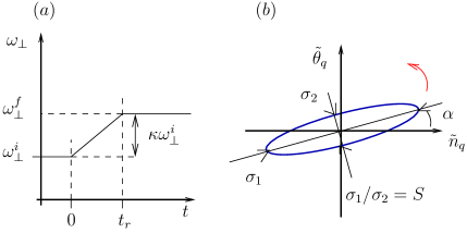
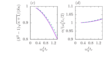
Figure 9: Effect of the interaction strength ramp on the squeezing of longitudinal modes. The time sequence is shown in $(a)$. An example of the phase space distribution at the end of the ramp is shown in $(b)$: the $1/\sqrt{e}$ line of the Gaussian distribution is plotted. The squeezing factor $S$ is the ratio between the rms widths along the anti-squeezed and the squeezed directions. The curved arrow shows the direction of rotation under free evolution. Quantitative results are shown in $(c)$ and $(d)$ for a quench strength $\kappa=\omega_{\perp}^{f}/\omega_{\perp}^{i}-1=2$ (solid lines) and $\kappa=4$ (dashed lines). $(c)$ shows $\sqrt{\kappa+1}(S^{2}-1)/(S\kappa)$, which gives the amplitude of the resulting breathing oscillations normalized to the amplitude for an instantaneous quench (see text), versus $\omega_{q}^{f}t_{r}$ where $\omega_{q}^{f}$ is the final frequency of the mode. The squeezing angle is shown in $(d)$, normalized by $\omega_{q}^{f}t_{r}/2$.

The post-quench dynamics results in a breathing of the $\tilde{\theta}_{q}$ quadrature: $\langle\tilde{\theta}_{q}^{2}\rangle$ oscillates with an amplitude $V(S^{2}-1)/S$. Coming back to the variable ${\theta}_{q}$, the evolution at times $t>t_{r}$ writes

$$\langle{\theta}_{q}^{2}\rangle(t)=\langle{\theta}_{q}^{2}\rangle_{i}\frac{\sqrt{\kappa+1}}{S_{q}}\left(1+(S_{q}^{2}-1)\sin^{2}(\omega_{q}^{f}(t-t_{r})+\alpha_{q})\right)$$ (41)

where the indice $q$ in $S$ and $\alpha$ indicates these quantities depend on $q$. As seen in Fig. (9), the angle $\alpha_{q}$ is very close to $\omega_{q}^{f}t_{r}/2$, for moderate values of $\omega_{q}^{f}t_{r}$. Injecting this value into Eq. (41), we find that it amounts to shifting the time reference to $t_{r}/2$. We perform this shift when analyzing the data, in other terms the reduced variable $\tau$ is $\tau=cq(t-t_{r}/2)$.

Let us now consider the evolution of the density-ripples power spectrum $\langle|\tilde{\rho}_{q}|^{2}\rangle(t)$. For small $q$, $\langle|\tilde{\rho}_{q}|^{2}\rangle(t)$ is proportional to $\langle{\theta}_{q}|^{2}\rangle(t)$ such that the evolution of $\langle|\tilde{\rho}_{q}|^{2}\rangle(t)$ is given by Eq. (41). This leads to,

$$J(q,\tau)=\frac{\sqrt{\kappa+1}}{S_{q}}\left(1+(S_{q}^{2}-1)\sin^{2}(\tau)\right).$$ (42)

Let us now investigate the quantity $\bar{J}(\tau)$, defined in the main text for experimental data. Here we will assume that the measurement times are spread over $[t_{m},t_{M}]$ and we denote $h(t)dt$ the number of points in the time interval $[t,t+dt]$. The $q$ values are assumed to be equally spaced, as in the case of a Fast Fourier Transform, and only $q$ values in the interval $[q_{m},q_{M}]$ are considered. We assume that $\bar{J}(\tau)$ is obtained by binning in $\tau$ the collection of data with a bin size $\Delta$ small enough so that, for all measurement times $t$, $J(q,\tau)$ is about constant in the interval $q\in[\tau/(ct),(\tau+\Delta)/(ct)]$. Then, one has

$$\bar{J}(\tau)=\frac{1}{\int h(t)dt\Delta/(ct)}\int h(t)dtJ(q=\tau/(ct),\tau)\Delta/(ct),$$ (43)

where the integrals are evaluated between $t_{1}$ and $t_{2}$, where $t_{1}=\rm{Max}(t_{m},\tau/(cq_{M}))$ and $t_{2}=\rm{Min}(t_{M},\tau/(cq_{m}))$. Typically, in the experiment small times are sampled more densely than large times. Taking $h$ proportional to $1/t$, we obtain

$$\bar{J}(\tau)=\frac{1}{\int dt/t^{2}}\int dt\frac{J(q=\tau/(ct),\tau)}{t^{2}}=\frac{\int dqJ(q,\tau)}{q_{2}(\tau)-q_{1}(\tau)},$$ (44)

where $q_{1}=\rm{max}(\tau/(c)t_{M},q_{m})$ and $q_{2}=\rm{min}(\tau/(c)t_{m},q_{M})$.

The predicted time evolution of $\bar{J}$ is shown in Fig. (10) for parameters close to that of the experimental data shown in the main text. The amplitude of the first oscillation is decreased by about 10%.

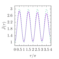
Figure 10: Effect of the finite ramp time of the interaction strength for a homogeneous gas. The expected behavior of $\bar{J}$ (solid line) is compared to the case of an instantaneous ramp (dashed line). Here we consider a gas of Rubidium atoms at conditions close to the experimental ones. More precisely, the linear density is $n_{0}=630$ atoms per $\mu$m, the initial transverse oscillation frequency is $\omega_{\perp}=2\pi\times 1.5$ kHz, the quench strength is $\kappa=2$ and the ramp time is $t_{r}=0.7$ ms. The range of $q$ values used to compute $\bar{J}$ is $q\in[0.1,0.5]\mu$m^-1 and the range of measurement times is $t\in[t_{r}/2,6$ms$]$.

H.2 Finite width of the convolution function used in data processing

The data shown in the inset of Fig. (3) of the main text correspond to a data set with an exceptionally good signal over noise. In general, the spread of the data points corresponding to a given value of $\tau$ (and thus corresponding to different times $t$ and wavevectors $q$) is as large as about 50%. In such conditions, a binning of the data as a function of the reduced time $\tau=cqt$ with a bin size sufficiently large to accommodate many data points is required in order to increase the signal over noise. As describe in the main text, we use a “smooth” binning: we compute the weighted average of the data, $\bar{J}$, with a Gaussian cost function of rms width $\Delta$. For a very dense data set, we can define the local average value $\tilde{J}(\tau)=\sum_{i,\tau_{i}\in[\tau,\tau+d\tau]}J_{i}/d\tau$, where the sum is done on the data set and $d\tau$ is much smaller than $\Delta$. Then $\bar{J}$ corresponds to the convolution of $\tilde{J}$ with a convolution width $\Delta$. This convolution reduces the amplitude of the oscillations. To estimate this amplitude reduction, let us disregard the small damping of the oscillations coming from the cloud inhomogeneity (see section 3) and thus consider data which would follow the oscillatory behavior $\tilde{J}=A\sin^{2}(\tau)$. The smoothing $\bar{J}(\tau)=\int_{-\infty}^{\infty}\!d\tau^{\prime}\tilde{J}(\tau^{\prime})\,e^{-\left(\tau^{\prime}-\tau\right)^{2}/(2\Delta^{2})}/(\sqrt{2\pi\Delta^{2}})$ reduces the amplitude to $A^{\prime}=Ae^{-2\Delta^{2}}$. For $\Delta=0.1\pi$, as used for the data analysis shown in the main text, the amplitude is reduced by 18%.

References

- [1] Anatoli Polkovnikov, Krishnendu Sengupta, Alessandro Silva, and Mukund Vengalattore. Colloquium: Nonequilibrium dynamics of closed interacting quantum systems. Rev. Mod. Phys., 83(3):863–883, August 2011.
- [2] See [42] and references therein.
- [3] S. Trotzky, Y.-A. Chen, A. Flesch, I. P. McCulloch, U. Schollwöck, J. Eisert, and I. Bloch. Probing the relaxation towards equilibrium in an isolated strongly correlated one-dimensional Bose gas. Nature Physics, 8(4):nphys2232, February 2012.
- [4] Marc Cheneau, Peter Barmettler, Dario Poletti, Manuel Endres, Peter Schauß, Takeshi Fukuhara, Christian Gross, Immanuel Bloch, Corinna Kollath, and Stefan Kuhr. Light-cone-like spreading of correlations in a quantum many-body system. Nature, 481(7382):484–487, January 2012.
- [5] Chen-Lung Hung, Victor Gurarie, and Cheng Chin. From Cosmology to Cold Atoms: Observation of Sakharov Oscillations in a Quenched Atomic Superfluid. Science, 341(6151):1213–1215, September 2013.
- [6] Tim Langen, Thomas Schweigler, Eugene Demler, and Jörg Schmiedmayer. Double light-cone dynamics establish thermal states in integrable 1d Bose gases. arXiv:1709.05994 [cond-mat, physics:quant-ph], September 2017. arXiv: 1709.05994.
- [7] J.-C. Jaskula, G. B. Partridge, M. Bonneau, R. Lopes, J. Ruaudel, D. Boiron, and C. I. Westbrook. Acoustic Analog to the Dynamical Casimir Effect in a Bose-Einstein Condensate. Phys. Rev. Lett., 109(22):220401, November 2012.
- [8] Jacopo De Nardis, Bram Wouters, Michael Brockmann, and Jean-Sébastien Caux. Solution for an interaction quench in the Lieb-Liniger Bose gas. Phys. Rev. A, 89(3):033601, March 2014.
- [9] Pasquale Calabrese and Pierre Le Doussal. Interaction quench in a Lieb–Liniger model and the KPZ equation with flat initial conditions. J. Stat. Mech., 2014(5):P05004, 2014.
- [10] M. A. Cazalilla and Ming-Chiang Chung. Quantum quenches in the Luttinger model and its close relatives. J. Stat. Mech., 2016(6):064004, 2016.
- [11] Tomasz Świsłocki and Piotr Deuar. Quantum fluctuation effects on the quench dynamics of thermal quasicondensates. J. Phys. B: At. Mol. Opt. Phys., 49(14):145303, 2016.
- [12] Bernhard Rauer, Sebastian Erne, Thomas Schweigler, Federica Cataldini, Mohammadamin Tajik, and Jörg Schmiedmayer. Recurrences in an isolated quantum many-body system. arXiv:1705.08231 [cond-mat, physics:quant-ph], May 2017. arXiv: 1705.08231.
- [13] Christophe Mora and Yvan Castin. Extension of Bogoliubov theory to quasicondensates. Phys. Rev. A, 67(5):053615, May 2003.
- [14] M. Schemmer, A. Johnson, R. Photopoulos, and I. Bouchoule. Monte Carlo wave-function description of losses in a one-dimensional Bose gas and cooling to the ground state by quantum feedback. Phys. Rev. A, 95(4):043641, April 2017.
- [15] For each positive value, one has 2 Fourier components: and , with similar expressions for . We omit the subscript or in the text for simplicity.
- [16] For quasi-1D gases the hydrodynamic condition is replaced by .
- [17] The phase space area is preserved, one quadrature being squeezed, while the other is anti-squeezed.
- [18] For the values considered, and the Raighley-Jeans approximation holds.
- [19] In [5], the evolution of density fluctuations has however been investigated for a 2D gas.
- [20] Isolating the contribution of individual modes to the function requires looking at the Fourier transform of , which requires large detection dynamics.
- [21] A. Imambekov, I. E. Mazets, D. S. Petrov, V. Gritsev, S. Manz, S. Hofferberth, T. Schumm, E. Demler, and J. Schmiedmayer. Density ripples in expanding low-dimensional gases as a probe of correlations. Phys. Rev. A, 80(3):033604, September 2009.
- [22] S. Dettmer, D. Hellweg, P. Ryytty, J. J. Arlt, W. Ertmer, K. Sengstock, D. S. Petrov, G. V. Shlyapnikov, H. Kreutzmann, L. Santos, and M. Lewenstein. Observation of Phase Fluctuations in Elongated Bose-Einstein Condensates. Phys. Rev. Lett., 87(16):160406, October 2001.
- [23] S. Manz, R. Bücker, T. Betz, Ch. Koller, S. Hofferberth, I. E. Mazets, A. Imambekov, E. Demler, A. Perrin, J. Schmiedmayer, and T. Schumm. Two-point density correlations of quasicondensates in free expansion. Phys. Rev. A, 81(3):031610, March 2010.
- [24] B. Rauer, P. Grišins, I. E. Mazets, T. Schweigler, W. Rohringer, R. Geiger, T. Langen, and J. Schmiedmayer. Cooling of a One-Dimensional Bose Gas. Phys. Rev. Lett., 116(3):030402, January 2016.
- [25] For consistency we rederive this expression (first established in [21]) see Appendix B,C.
- [26] In Eq. (5), where and are the cosine and sine Fourier components, which fulfill for translationally invariant systems.
- [27] Validity of LDA is established in Appendix E.
- [28] The experiment is described in more detail in [43].
- [29] K. V. Kheruntsyan, D. M. Gangardt, P. D. Drummond, and G. V. Shlyapnikov. Pair Correlations in a Finite-Temperature 1d Bose Gas. Phys. Rev. Lett., 91(4):040403, July 2003.
- [30] J. N. Fuchs, X. Leyronas, and R. Combescot. Hydrodynamic modes of a one-dimensional trapped Bose gas. Phys. Rev. A, 68(4):043610, October 2003.
- [31] the box is chosen to be about twice the size of the cloud.
- [32] The transverse size of the cloud after the time-of-flight is comparable to the depth of focus of the imaging system and depends on the transverse confinement. We thus expect slightly different optical resolutions, and for data taken before and after the quench respectively. We correct for this effect to make quantitative comparison of data taken before and after the quench.
- [33] The values of resolution obtained by such fits are close to the expected values if one takes into account the depth of field of our imaging system and the fact that, after the the expansion time the cloud explores about 50m along the imaging direction.
- [34] Thibaut Jacqmin, Julien Armijo, Tarik Berrada, Karen V. Kheruntsyan, and Isabelle Bouchoule. Sub-Poissonian Fluctuations in a 1d Bose Gas: From the Quantum Quasicondensate to the Strongly Interacting Regime. Phys. Rev. Lett., 106(23):230405, June 2011.
- [35] At a time the function has reached the thermal value for all , the deviation from this thermal state being restricted to long distances where .
- [36] A. Johnson, S. S. Szigeti, M. Schemmer, and I. Bouchoule. Long-lived nonthermal states realized by atom losses in one-dimensional quasicondensates. Phys. Rev. A, 96(1):013623, July 2017.
- [37] We corrected the formula published in [21].
- [38] D. Hellweg, S. Dettmer, P. Ryytty, J. J. Arlt, W. Ertmer, K. Sengstock, D. S. Petrov, G. V. Shlyapnikov, H. Kreutzmann, L. Santos, and M. Lewenstein. Phase fluctuations in Bose–Einstein condensates. Appl Phys B, 73(8):781–789, December 2001.
- [39] This term is due to the approximation made when going from Eq. (7) to Eq. (8), which is valid only for values larger than the inverse of the cloud size.
- [40] Since the Hamiltonian of interest is quadratic in , the distribution of is Gaussian at thermal equilibrium. The squeezing of each collective mode produced by the interaction quench preserves the Gaussian nature of .
- [41] M. Olshanii. Atomic Scattering in the Presence of an External Confinement and a Gas of Impenetrable Bosons. Phys. Rev. Lett., 81(5):938–941, August 1998.
- [42] Aditi Mitra. Quantum quench dynamics. arXiv:1703.09740 [cond-mat], March 2017. arXiv: 1703.09740.
- [43] Thibaut Jacqmin, Bess Fang, Tarik Berrada, Tommaso Roscilde, and Isabelle Bouchoule. Momentum distribution of one-dimensional Bose gases at the quasicondensation crossover: Theoretical and experimental investigation. Phys. Rev. A, 86(4):043626, October 2012.