Barotropic theory for the velocity profile of Jupiter turbulent jets: an example for an exact turbulent closure

Abstract

We model the dynamics of Jupiter’s jets by the stochastic barotropic beta-plane model. In this simple framework, by analytic computation of the averaged effect of eddies, we obtain three new explicit results about the equilibrium structure of jets. First we obtain a very simple explicit relation between the Reynolds stresses, the energy injection rate, and the averaged velocity shear. This predicts the averaged velocity profile far from the jet edges (extrema of zonal velocity). Our approach takes advantage of a timescale separation between the inertial dynamics on one hand, and the spin up (or spin down) time on the other hand. Second, a specific asymptotic expansion close to the eastward jet extremum explains the formation of a cusp at the scale of energy injection, characterised by a curvature that is independent from the forcing spectrum. Finally, we derive equations that describe the evolution of the westward tip of the jets. The analysis of these equations is consistent with the previously discussed picture of barotropic adjustment, explaining the relation between the westward jet curvature and the beta effect. Our results give a consistent overall theory of the stationary velocity profile of inertial barotropic zonal jets, in the limit of small scale forcing.

1 Introduction

The giant gaseous planets like Jupiter and Saturn can be seen as paradigmatic systems to study geostrophic turbulent flows (see (Vasavada & Showman, 2005) for Jupiter). Gallileo and Cassini gave high resolution observations of Jupiter’s troposphere dynamics (Salyk et al., 2006; Porco et al., 2003). The large alternating colored bands at the top of the troposphere are correlated with the zonal wind vorticity. Vortices with a scale of about a thousand kilometers often appear after three dimensional convective activity in the atmosphere. The interaction between those vortices and the zonal jets continuously transfers energy to the barotropic component (Ingersoll et al., 1981; Salyk et al., 2006), and equilibrates the dissipation mechanisms. The dynamics of large scale jet formation may be qualitatively well understood within the framework of two-dimensional geostrophic turbulence in a $\beta$ plane (Pedlosky, 1982), although more refined models are needed to understand their quantitative features (Li et al., 2006; Schneider & Liu, 2009). As the aim of this work is to make progresses in the theoretical understanding of turbulent flows, we consider geostrophic turbulence in the simple barotropic $\beta$ plane model. Despite all its limitations, for instance the lack of dynamical effects related to baroclinic instabilities, we will show that this model reproduces the main qualitative features of the velocity profiles.

An interesting property of two dimensional turbulent flows is their inverse energy transfer from small scales to large scales, sometimes through a cascade among scales, but much more often through a direct transfer from small scale to large scale mediated by the large scale flow. This inverse energy transfer is responsible for the self organization of the flow into large scale coherent structures that may evolve much slower than the eddies. Among those structures, giant vortices and zonal jets have raised strong interest in the scientific community. The $\beta$ effect favors the formation of jets, but without $\beta$ effect both jets and vortices can be observed in numerical simulations  (Sommeria, 1986; Bouchet & Simonnet, 2009; Frishman et al., 2017). Both structures are also observed in the atmosphere of gaseous planets (Ingersoll, 1990; Galperin et al., 2014, 2001). The computation of statistical equilibrium theory of the two-dimensional Euler and quasi-geostrophic equations (Bouchet & Venaille, 2012), using large deviation theory, led to the conclusion that zonal jets as well as large vortices are stable equilibrium states of the flow, and thus natural attractors. However, planetary flows are continuously damped and forced and a non-equilibrium theory must explain the selection between all such possible attractors.

The exact shape of zonal winds on Jupiter reveals an astonishing asymmetry between eastward jets and westward jets (Porco et al., 2003; Sánchez-Lavega et al., 2008; Garcí et al., 2001). Whereas eastward jets form cusps at their maximum velocity, westward jets are smoother, close to a parabolic velocity profile. At the same time, the profile of potential vorticity (PV) looks like “staircases” (Dritschel & McIntyre, 2008), and all those prominent features are well reproduced in direct numerical simulations of $\beta$ plane turbulence. One could ’postulate’ a potential vorticity staircase profile and derive the corresponding mean flow (Dritschel & McIntyre, 2008). This exercice is very enlightening, as it roughly relates jet spacing to other flow properties. Nevertheless, the physical mechanism leading to the staircase profile remains unclear. Moreover as our discussion will clearly show, the potential vorticty staircase is just a useful idealised approximation: the actual jet profile will depend on the control parameters, for instance friction, force spectrum, and $\beta$.

Starting from the stochastic barotropic beta plane model, our aim is to derive simple general relations for the jet velocity profile. A promising nonequilibrium statistical theory explaining jet formation is the stochastic structural stability (S3T) theory (Farrell & Ioannou, 2003, 2007) or the closely related second order cumulant expansion theory (CE2) (Marston et al., 2008). The key ingredient in those theories is to neglect eddy-eddy interactions, keeping only the interaction between eddies and the mean flow. With this quasilinear approximation, there is no inverse energy cascade in Fourier space anymore, and the inverse energy flux goes through interactions with the mean flow. This may be relevant only when the inverse energy cascade flux are negligible. The flow governed by the S3T equations, with or without phenomenological added stochastic forcing, produces spontaneous emergence and equilibration of zonal jets (Bakas & Ioannou, 2013; Constantinou et al., 2012) which velocity profiles reproduce quite well the main features of jets obtained in rotating-tank experiments (Read et al., 2004), numerical experiments (Vallis & Maltrud, 1993; Williams, 1978) or in the atmosphere of gaseous planets.

The question of why and when this quasilinear approximation should give such good results has been addressed in (Bouchet et al., 2013). The main result is that the quasilinear approximation is self-consistent in the inertial limit of weak stochastic forcing and dissipation, when the inertial time scale is much smaller than the spin up or spin down time scale. For Jupiter the inertial time scale is of order of a day or a month, while the spin up or spin down time scale, related to dissipative phenomena (radiative balance on Jupiter) may be of order of ten years (see e.g (Porco et al., 2003)). Moreover it follows from (Bouchet et al., 2013) analysis that the quasilinear equations are expected to be valid above a crossover scale, that tends to zero in the limit of weak stochastic forces and dissipation limit. Using this justified approximation in the inertial limit, it is then possible to write a closed equation for the evolution of the mean velocity.

If we assume that all the energy injected by the force is locally transferred to the mean flow, we obtain

$$\left\langle uv\right\rangle=\frac{\epsilon}{U^{\prime}},$$ (1)

where $U$ is the mean zonal velocity profile, $U^{\prime}$ its derivative with respect to the South-North coordinate $y$, $\left\langle uv\right\rangle$ the Reynolds stress, and $\epsilon$ the energy injection rate per unit of mass. Such a formula for the Reynolds stress might give a closed equation for the zonal jet, and is consequently very appealing. This expression is very similar to the one discussed in (Laurie et al., 2014) for a vortex without $\beta$ effect. In this paper this formula was obtained by neglecting the pressure term and the cubic terms in the energy balance relation, without justification. A more general formula, taking into account possible small scale dissipation, was actually obtained previously by (Srinivasan & Young, 2014), through explicit computation assuming a constant shear flow $U^{\prime}=Cst$. A similar result also holds in the case of dipoles for the 2D Navier–Stokes equations (Kolokolov & Lebedev, 2016a, b). Through numerical computations (Laurie et al., 2014) have shown that the analogous result for the 2D Navier–Stokes equations actually predicts correctly the velocity profile in a restricted part of the domain, far from the core of the vortex and far from the flow separatrix. (Kolokolov & Lebedev, 2016a) give scaling arguments to show in which domain of the flow the theoretical expression for the velocity profile is expected to hold.

In section 3, following preliminary results in (Woillez & Bouchet, 2017), we prove that equation (1) can be deduced as a consequence of the two limits of weak forces and dissipation on one hand, and of small scale forcing on the other hand. This first result justifies equation (1) and clarifies the required hypothesis. By contrast with our previous work (Woillez & Bouchet, 2017), in the present paper we discuss completely the mathematical justification when taking the limit of small scale forces before the inertial limit of weak forces and dissipation. The other order for these limits is way simpler mathematically, but is not relevant for turbulent flows.

In section 3.3, we use result (1) to write a closed equation for the mean velocity profile $U$. We solve it for the resulting stationary profile. With such an equation, the stationary profile diverges at some finite latitude. We thus conclude that the appealing formula (1) is valid only far from the jet tips, where $U^{\prime}$ does vanish. A more refined analysis is required to deal with the zonal jet velocity extrema.

In section 4, using Laplace transform tools, we derive an equation for the Reynolds stress divergence in the inertial limit. Taking afterwards the small-scale forcing limit, we give a set of equations that describes the zonal velocity extremum of the eastward jet. Although the full numerical calculation of the solution is avoided, we give some arguments to show that this set of equations leads to the formation of a “cusp” of typical size $\frac{1}{K}$ where $\frac{1}{K}$ is a typical scale of the stochastic forcing. We explain that this cusp has no universal shape: it depends on the stochastic forcing spectrum and on the dissipative mechanism. Yet we derive a relation, valid when viscous phenomena are negligible at the size of the cusp, that relates the curvature of the cusp to the maximal velocity $U(y_{cr})$. It writes

$$U(y_{cr})U^{\prime\prime}(y_{cr})=-\frac{\epsilon K^{2}}{r},$$ (2)

where $r$ is the linear friction coefficient in $s^{-1}$ (see equation (34)). Remarkably this relation does not depends on the forcing spectrum, but just on $\epsilon$.

On the contrary, the westward jet cannot form this cusp because it would violate the Rayleigh-Kuo criterion of stability. In section 5, we derive a self-consistent equation for the westward jet extrema. We explain that an instability can develop at the extremum, and how it stops the westward jet growth such that the zonal flow form a parabolic profile of curvature about $\beta$. This is compatible with the classical idea of barotropic adjustment. We also demonstrate that the appearance of neutral modes (modified Rossby waves) is not sufficient to arrest the growth of the jet extremum velocity, and that a marginal and transient instability is necessary.

2 Reynolds stresses from energy, enstrophy, and pseudomomentum balances

2.1 The stochastic barotropic $\beta$ plane model

We start from the equations for a barotropic flow on a periodic beta plane with stochastic forces

$$\partial_{t}\Omega+V.\nabla\Omega = -r\Omega-\beta_{d}V_{y}+\sqrt{2\epsilon}\eta$$ (3)

$$\nabla.V = 0,$$

where the vorticity $\Omega:=\left(\nabla\wedge V\right).e_{z}$ is the curl of the two dimensional velocity field $V:=\begin{pmatrix}V_{x}\\ V_{y}\end{pmatrix}$, $r$ models a linear friction, $x$ and $y$ are the East–West and North–South coordinates respectively, $\beta_{d}$ the Coriolis parameter, and $\eta$ is a stochastic force that we assume white in time: $\mathbb{E}\left[\eta(x,y,t)\eta(x^{\prime},y^{\prime},t^{\prime})\right]=\delta(t-t^{\prime})C_{d}(x-x^{\prime},y-y^{\prime\prime})$. We assume that $C_{d}$ is statistically homogeneous such that it depends only on the difference $x-x^{\prime}$ and $y-y^{\prime}$. We choose a particular normalization for the correlation function $C_{d}$, such that $\epsilon$ is the energy injection rate per unit mass: $\epsilon$ has dimensions $m^{2}s^{-3}$. In the following, we will always assume that there is no direct energy injection in the zonal velocity profile, i.e that $\frac{1}{L_{x}}\int{\rm d}x\eta(r,t)=0.$

Nondimensional equations and nondimensional numbers are the clearest way to determine the flow regime. We choose here to set temporal and spatial units such that the mean kinetic energy is 1, and $L_{x}=1$ (please see (Bouchet et al., 2013) for more details, or (Bouchet et al. (2016) page 2-3) for comparison with other common nondimensionalizations of the stochastic barotropic equations). For simplicity, we use the same notations for the dimensional and nondimensional velocity and vorticity. The nondimensional equations are

$$\partial_{t}\Omega+V.\nabla\Omega = -\alpha\Omega-\beta V_{y}+\sqrt{2\alpha}\eta,$$ (4)

$$\nabla.V = 0.$$

Now $\alpha=L\sqrt{r^{3}/\epsilon}$ is a nondimensional parameter although we will often refer to it as the “friction”. $\beta=\sqrt{r/\epsilon}L^{2}\beta_{d}$ is the new nondimensional Coriolis parameter, while $\beta_{d}$ is the dimensional one. We note that $\beta=L^{2}/L_{R}^{2}$, where $L_{R}=\left({\epsilon/r\beta_{d}^{2}}\right)^{1/4}$ is the Rhines scale. The zonostrophy index used in many references would be $R_{\beta}=\beta^{1/10}\epsilon^{1/20}r^{-1/4}$. We find that $\alpha\propto(R_{\beta})^{-5}$, which implies that the inertial limit of vanishing $\alpha$ corresponds to the limit of large $R_{\beta}$. Let $C(r)$ be the nondimensional expression of the noise correlation function $C_{d}(r)$. We denote $\hat{C}_{k,l}$ the Fourier coefficients of $C$,

$$C(x,y):=\underset{k,l}{\sum}\hat{C}_{k,l}e^{ikx+ily},$$ (5)

and $K^{2}=k^{2}+l^{2}$. As a correlation function, $C$ is a definite positive function and as a conseuence $\hat{C}_{k,l}$ is real and positive. Moreover, if we assume the symmetry $x\rightarrow-x$ and $y\rightarrow-y$, the function $\hat{C}_{k,l}$ is symmetric with respect to $k\rightarrow-k$ and $l\rightarrow-l$. The constrain that the mean kinetic energy is one writes

$$\frac{1}{2}\iint{\rm d}k{\rm d}l\frac{\hat{C}_{k,l}}{K^{2}}=1.$$ (6)

From now on, the computations will be done with nondimensional quantities. If we want to write a result in its dimensional formulation, we will reintroduce $\left[\frac{\epsilon}{r}\right]=m^{2}.s^{-2}$ and $[L_{x}]=m$.

We separate the flow $V$ in two parts, $V(r,t)=U(y,t)e_{x}+\begin{pmatrix}u(r,t)\\ v(r,t)\end{pmatrix}$. The mean velocity $Ue_{x}=\left\langle V\right\rangle$ is defined as the zonal and stochastic average of the velocity field. More precisely, we assume that the mean flow is parallel and we take $\left\langle V\right\rangle=\frac{1}{L_{x}}\int{\rm d}x\mathbb{E}[V(x,y)]$. In the following, the bracket $\left\langle\right\rangle$ will be used for both the zonal and stochastic averages. The vorticity then separates in $\Omega(r,t)=-U^{\prime}(y,t)+\omega(r,t)$, where the prime denotes the derivative with respect to $y$. We will refer to $U$ indifferently as the mean flow or zonal flow.

Using this decomposition and the continuity equation, we can obtain an equation for the zonal component of the vorticity, and then integrate over $y$ to get the equation for the mean velocity $U$

$$\partial_{t}U+\partial_{y}\left\langle uv\right\rangle=-rU.$$ (7)

Equation (7) shows that the mean flow is forced by the divergence of the Reynolds stress $\partial_{y}\left\langle uv\right\rangle$. In order to reach an equilibrium, this latter term has to balance the dissipation coming from linear friction.

2.2 Quasilinear approximation and pseudomomentum balance

In this section we define the quasilinear approximation. We recall basic concepts about linear dynamics and the relation between stochastic and deterministic linear dynamics.

In the following we are interested in the small $\alpha$ regime (the inertial or weak forces and dissipation regime). In the limit where $\alpha$ goes to zero in equation (4), we can neglect the nonlinear eddy-eddy interactions. This approximation is called the quasilinear approximation. The quasilinear approximation has been shown self-consistent by (Bouchet et al., 2013) with some assumptions on the profile $U$ (stability, no zero modes). We will not develop the full justification of the quasilinear approximation here, the interested reader is referred to (Bouchet et al., 2013). Let us simply recall the heuristic ideas leading to the quasilinear approximation. First, we notice that the strength of the noise is of order $\sqrt{\alpha}$. As fluctuations are sheared and transferred to the largest scales on a timescale of order one, this is a natural hypothesis to expect fluctuations $(u,v)$ to be of the same order. This was proven to be self-consistent in (Bouchet et al., 2013). We make the rescaling $(u,v):=\sqrt{2\alpha}(u^{\prime},v^{\prime})$ in equation (4), and we omit the prime in the following for clarity. The eddy-eddy interaction terms are of order $\alpha^{\frac{3}{2}}$, and can then be neglected. We are left with the set of equations

$$\partial_{t}U=-\alpha\left[\partial_{y}\left\langle uv\right\rangle+U\right]$$ (8)

$$\partial_{t}\omega+U\partial_{x}\omega+(\beta-U^{\prime\prime})v=-\alpha\omega+\eta$$ (9)

where $\omega=\partial_{x}v-\partial_{y}u=\triangle\psi$ is the rescaled vorticity fluctuations. Equation (8) shows that the typical timescale for the evolution of the mean flow $U$ is $\frac{1}{\alpha}$. By contrast, equation (9) shows that the timescale for eddy dynamics is of order one. Using this timescale separation, we will consider that $U$ is a constant field in the second equation (9), and we will solve $\omega(t)$ for a given profile $U$. Once $U$ is considered as given, the eddy equation is linear. This time scale separation is observed for example on Jupiter where the typical time of eddies evolution ranges from few days to few weeks whereas significant changes in the mean flow are only detected over decades (see e.g (Porco et al., 2003)).

Without forces and dissipation, the quasilinear equations conserve energy and enstrophy as do the full barotropic flow equations. One of the key relations we will use in this paper comes from the fluctuation enstrophy balance

$$\frac{1}{2}\partial_{t}\left\langle\omega^{2}\right\rangle-(\beta-U^{\prime\prime})\partial_{y}\left\langle uv\right\rangle=-\alpha\left\langle\omega^{2}\right\rangle+\frac{1}{2}C(0).$$

where we have used

$$\left\langle v\omega\right\rangle=-\partial_{y}\left\langle uv\right\rangle,$$ (10)

which a consequence of incompressibility.

As a consequence, if $U^{\prime\prime}-\beta$ has a constant sign in the flow, without forces and dissipation, the left-hand side of equation (9) conserves the pseudomomentum $\int\frac{\left\langle\omega^{2}\right\rangle}{U^{\prime\prime}-\beta}\rm{d}y$. The pseudomomentum does not allow any instability to occur and the flow is stable. This is called the Rayleigh-Kuo criterion for stability of shear flows. If $U^{\prime\prime}-\beta$ vanishes somewhere in the flow, an instability may or may not exist. The fact that $U^{\prime\prime}-\beta$ vanishes is a necessary condition for instability, not a sufficient one.

As we assume a timescale separation between the zonal flow and fluctuation dynamics, we are interested in the long-term behavior of the Reynolds stress $\partial_{y}\left\langle uv\right\rangle$. When the vorticity fluctuations $\omega$ reach its stationary distribution, we have the relation

$$\partial_{y}\left\langle uv\right\rangle=-\frac{1}{U^{\prime\prime}-\beta}\left[\alpha\left\langle\omega^{2}\right\rangle-\frac{1}{2}C(0)\right].$$ (11)

This equation for the Reynolds stress will be extremely useful.

We now take the Fourier transform of (9) in $x$: $\omega_{k}(y):=\frac{1}{L_{x}}\int{\rm d}x\omega(x,y)e^{-ikx}$ with $k$ taking the values $\frac{2\pi}{L_{x}}n$, $n$ is an integer. We also use the linearity to express the solution as the sum of particular solutions for independent stochastic forcings $\eta_{l}(y,t)$. We denote $\omega_{k,l}(y,t)$ the solution of

$$\partial_{t}\omega_{k,l}+L_{k}[\omega_{k,l}]=-\alpha\omega_{k,l}+\eta_{l},$$

where

$$L_{k}[\omega_{k,l}]=ikU\omega_{k,l}+ik(\beta-U^{\prime\prime})\psi_{k,l},$$ (12)

and where $\eta_{l}$ is a Gaussian white noise with correlations $\mathbb{E}\left[\eta_{l}(y,t)\eta_{l}(y^{\prime},t)\right]=e^{il(y-y^{\prime})}\delta(t-t^{\prime})$. From equation (11) we obtain

$$\partial_{y}\left\langle uv\right\rangle=-\frac{1}{U^{\prime\prime}-\beta}\underset{k,l}{\sum}\frac{\hat{C}_{k,l}}{2}\left[2\alpha\left\langle|\omega_{k,l}|^{2}\right\rangle-1\right],$$ (13)

where the positive constants $\hat{C}_{k,l}$ are defined by (5). We stress that in this formula the bracket $\left\langle|\omega_{k,l}|^{2}\right\rangle$ denotes a stochastic average, because the zonal average is already taken into account by the sum over all vectors $k$.

We now proceed to a further simplification, showing that the stochastic eddy dynamics can be computed from a set of deterministic linear problems, following (Bouchet et al., 2013). We use that equation (12) is a linear operator for a given $U$ and that the noise $\eta_{k,l}$ is white in time and has an exponential correlation function $c_{l}(y)=e^{ily}$ to express the stationary average $\left\langle|\omega_{k,l}|^{2}\right\rangle$ as

$$\left\langle|\omega_{k,l}|^{2}\right\rangle=\int_{-\infty}^{0}{\rm d}t~{}e^{2\alpha t}\left|e^{tL_{k}}[c_{l}]\right|^{2},$$ (14)

where $e^{tL_{k}}[c_{l}]$ is the solution at time $t$ of the deterministic equation

$$\partial_{t}\omega_{d}+L_{k}[\omega_{d}]=0,$$

with initial condition $c_{l}:=y\rightarrow e^{ily}$.

Equations (13), (14) and (8) give a way to compute Reynolds stresses and the velocity profile $U$ from classical and much studied deterministic hydrodynamic problems. Equation (15) is however tricky and has no simple explicit expression in the general case. We will be able to get explicit result only in asymptotic regimes.

2.3 Simplifications in asymptotic regimes

Expression (14) is still complicated because to get explicit results, it requires to know the behavior of the solution $e^{tL_{k}}[c_{l}]$ up to times of order $\frac{1}{\alpha}$. Two parameters can be used to further simplify the problem, the vector $\mathbf{k}=(k,l)$ and the damping $\alpha$. We denote $K:=|\mathbf{k}|$. We will be interested both in the regime $K\rightarrow\infty$ and $\alpha\rightarrow 0$. The large $K$ regime is a small scale forcing regime.

The inertial limit $\alpha\rightarrow 0$ is the most difficult one, because turbulence can develop on a very long time. But the inertial limit is also the most interesting from a physical point of view because it corresponds to fully turbulent regimes, and is the most relevant one to describe Jupiter’s atmosphere. In this section we prove that equation (13) and (14) can be further simplified and computed through the asymptotic behavior of a linear dynamics without dissipation, in the inertial regime.

The result in the inertial regime crucially depends on whether the deterministic equation without dissipation

$$\partial_{t}\omega_{d}+ikU\omega_{d}+ik(\beta-U^{\prime\prime})\psi_{d}=0$$ (15)

with initial condition $\omega_{d}(y,0)=c_{l}$, sustains neutral modes or not. A neutral mode is defined as a solution of this equation of the form $\omega_{d}(y,t)=\xi^{a}(y)e^{ic_{a}t}$ where $c_{a}$ is a real constant. It is also sometimes called “modified Rossby waves” in this context, when the jet velocity is nonzero. Two cases can be encountered. In the first case, without neutral modes, (Bouchet & Morita, 2010) have shown that $\omega_{d}$ behaves asymptotically for long time as $\omega_{d}(y,t)\underset{t\rightarrow\infty}{\sim}\omega^{\infty}(y)e^{ikUt}$, even for non monotonous velocity profiles $U$. Please note that we should write $\omega_{kl}^{\infty}(y)$ because the asymptotic limit of $\omega_{d}$ depends on the wavevector, but we choose to omit the indices $k,l$ for clarity. Moreover (Bouchet & Morita, 2010) give a method to compute this $\omega^{\infty}$ using Laplace transform tools. In this case, in the limit $\alpha\rightarrow 0$, the Reynolds stress writes

$$\partial_{y}\left\langle uv\right\rangle=-\frac{1}{U^{\prime\prime}-\beta}\underset{k,l}{\sum}\frac{\hat{C}_{k,l}}{2}\left[|\omega^{\infty}|^{2}-1\right].$$ (16)

We give the full justification of this result in appendix A.

In the second case, with neutral modes, we have to modify expression (16) to take into account the presence of modes. Again, we leave the technical details to appendice A and we give the final result

$$\partial_{y}\left\langle uv\right\rangle=-\frac{1}{U^{\prime\prime}-\beta}\underset{k,l}{\sum}\frac{\hat{C}_{k,l}}{2}\left[|\tilde{\omega}^{\infty}|^{2}-1+\underset{modes~{}a}{\sum}|\omega^{a}|^{2}\right].$$ (17)

This result means that we have to project first the initial condition $c_{l}$ over the modes labeled by $a$. The component over the $a$ mode gives the term $\omega^{a}(y)$. This new terms are related to the wave pseudomomentum balance. Then we compute the asymptotic solution $\tilde{\omega}^{\infty}$ of (15) using as initial condition not $c_{l}$ but $c_{l}-\sum\omega^{a}$. Briefly speaking, a first reason why there are no cross terms of the form $\omega^{a}\tilde{\omega}$ between modes and the remaining part of the spectrum is because the frequencies $c_{a}$ of the modes are always outside of the range of $U$ as shown by (Drazin et al., 1982; Pedlosky, 1964). The cross terms have an oscillatory part of frequency $\frac{1}{\alpha}(c_{a}-U)$ that gives a vanishing contribution in the small $\alpha$ limit.

Both formulas (16-17) are independent from $\alpha$ in the limit of vanishing $\alpha$. This is a non-trivial result. The formulas will be used to study the inertial limit in section 3.

3 Explicit velocity profile in the inertial and small scale forcing regime

Observations collected by the Gallileo and Cassini probes (see (Porco et al., 2003) and others) allows to estimate typical values for $K$ and $\alpha$. $1/K$ is the forcing length scale. It can be estimated to be or order $1000$ km, the typical size of cyclones due to convective activity in Jupiter’s troposphere. The dissipation on Jupiter involves different mechanisms, which are roughly modelled by our linear friction. What could is a relevant typical timescale for dissipation is not obvious. Based on Jupiter observations, many authors (Porco et al., 2003; Vasavada & Showman, 2005; Salyk et al., 2006) consider a large scale dissipation time $1/r$ of the order of a few years. To compute an order of magnitude for the non dimensional parameter $\alpha$, we have chosen $1/r=5$ years. $U$ is easily estimated from the observations, and the Coriolis parameter $\beta$ is easily computed from the rotation rate of Jupiter. After non-dimensionalisation, following the discussion in the previous section, we estimate the orders of magnitude for $K\sim 10$ and $\alpha\sim 10^{-3}$. Jupiter is thus in the asymptotic regime $\alpha\rightarrow 0$ and $K\rightarrow+\infty$. Both limits do not necessarily commute, we thus have to be careful which limit we are going to take first. The turbulent nature of the dynamics at the forcing scale suggests the limit $\alpha\rightarrow 0$ first, and then $K\rightarrow+\infty$.

3.1 Computation of the long-time limit of eddy vorticity

In the following and until section 5, we assume there are no Rossby waves in the flow. It has been shown long ago that those waves travel in a barotropic flow at a velocity $c<U_{min}$ (Drazin et al., 1982; Pedlosky, 1964). In section 5, we will explain how we can compute Rossby waves in case of a parabolic profile.

In this subsection, we summarize the main result obtained by Bouchet and Morita (Bouchet & Morita, 2010) that allows us to compute the function $\omega^{\infty}$ appearing in (16). $\omega^{\infty}$ gives then an easy access to the small $\alpha$ limit, independently of the large $K$ limit.

We start from equation (15) that describes the linear evolution of a perturbation $\omega(y,t)\mbox{e}^{ikx}$ of meridional wave number $k$, and with streamfunction $\psi(y,t){\rm e}^{ikx}$. In the following, we will stop using the subscript $d$ for the deterministic solution $\omega_{d}$ in (15). We introduce the function $\varphi_{\epsilon}(y,c)$ which is the Laplace transform of the stream function $\psi(y,t)$ i.e $\varphi_{\epsilon}(c):=\int_{0}^{\infty}{\rm d}t\psi(y,t)e^{ik(c+i\epsilon)t}$. To avoid any confusion, we stress that in this section, $\epsilon$ will always denote a small parameter and not the energy injection rate. The Laplace transform $\varphi_{\epsilon}$ is well defined for any non zero value of the real variable $\epsilon$ with a strictly positive product $k\epsilon$. $c$ has to be understood as the phase speed of the wave, and $k\epsilon$ is the exponential growth rate of the wave. Note that $k\epsilon$ exactly corresponds to a linear friction in equation (15), such that the inertial limit $\alpha\rightarrow 0$ is equivalent to the limit $\epsilon\rightarrow 0$. The equation for $\varphi_{\epsilon}$ is

$$\left(\frac{d^{2}}{dy^{2}}-k^{2}\right)\varphi_{\epsilon}(y,c)+\frac{\beta-U^{\prime\prime}(y)}{U(y)-c-i\epsilon}\varphi_{\epsilon}(y,c)=\frac{\omega(y,0)}{ik(U(y)-c-i\epsilon)},$$ (18)

(see (Bouchet & Morita, 2010)), with vanishing boundary conditions at infinity. We do not have an infinite flow in the $y$ direction, but the properties of the flow become local for large $K$. The choice to take vanishing boundary conditions at infinity is done for convenience and it is expected that this particular choice does not modify the physical behavior of the perturbation.

For all $\epsilon>0$ the function $\varphi_{\epsilon}$ is well defined. The inhomogeneous Rayleigh equation (18) is singular for $\epsilon=0$ at any critical point (or critical layer) $y_{c}$ such that the zonal velocity is equal to the phase speed: $U(y_{c})=c$. One can show that $\varphi_{\epsilon}$ has a limit denoted $\varphi_{+}$ when $\epsilon$ goes to zero. The function $\omega^{\infty}$ is then given by

$$\omega^{\infty}(y)=ik(U^{\prime\prime}(y)-\beta)\varphi_{+}(y,U(y))+\omega(y,0),$$ (19)

see (Bouchet & Morita, 2010). The function $\omega^{\infty}$ depends on the Laplace transform of the stream function but for a phase velocity $c$ equal to the zonal velocity at latitude $y$. From a mathematical point of view, it corresponds to the value of $\varphi_{+}$ exactly at its singularity. The singularity in equation (18) is of degree one (proportional to $\frac{1}{y}$) except at the extrema of the jets where it is of degree two. A singularity of order two would create a divergence for the solution, but it happens that the numerator in (18) vanishes at such points and the solution is still defined at the extrema of a jet. A nontrivial consequence of that is

$$\omega^{\infty}(y_{cr})=0$$

at all critical latitudes $y_{cr}$ where $U^{\prime}(y_{cr})=0.$ This result, called depletion of vorticity fluctuation at the jet critical points in (Bouchet & Morita, 2010), has important physical consequences that influence the dynamics of a jet.

As described in (Bouchet & Morita, 2010), using formula (18) and (19), one can numerically compute the function $\omega^{\infty}$ : we first have to solve a set of boundary value problems for ordinary differential equations parameterized by $c$ and $\epsilon$ to obtain a solution family $\varphi_{\epsilon}(c)$. Then we evaluate, for small enough $\epsilon$ each solution $\varphi_{\epsilon}(c)$ at the value $y_{c}$ satisfying $U(y_{c})=c$. This method is much faster and has less numerical cost than computing the long time evolution of the partial differential equation (15). We use this method in the following of this section.

3.2 Limit of small scale forcing for monotonic profiles, and explicit expression of the Reynolds stress

Again, we assume there are no Rossby waves. We will now consider the limit of small scale forcing $K\rightarrow\infty$. The calculations are rather technical and can be skipped in the first lecture. The result of this section is equation (22)

We start from equation (18) that describes the inertial behavior of a deterministic evolution of a perturbation $\omega(y,0)$ when $\epsilon$ vanishes. Using the Green function $H_{k}(y)$ of $(\partial_{y}^{2}-k^{2})$ we write

$$\varphi_{\epsilon}(y,c)=\left(U^{\prime\prime}(y)-\beta\right)\int{\rm d}y^{\prime}H_{k}(y^{\prime})\frac{\varphi_{\epsilon}(y-y^{\prime},c)}{U(y-y^{\prime})-c-i\epsilon}+\int{\rm d}y^{\prime}H_{k}(y^{\prime})\frac{\omega(y-y^{\prime},0)}{ik(U(y-y^{\prime})-c-i\epsilon)}.$$

Now we make the change of variable $Y=ky^{\prime}$ . The Green function has the scaling $H_{k}(y^{\prime}):=-\frac{1}{2k}H_{0}(Y)$. Recalling that $\varphi_{+}(y,c)=\lim_{\epsilon\downarrow 0}\varphi_{\epsilon}(y,c)$, it follows

$$\varphi_{+}(y,c)=-\frac{\left(U^{\prime\prime}(y)-\beta\right)}{2k^{2}}\underset{\epsilon\rightarrow 0}{\lim}\int{\rm d}YH_{0}(Y)\frac{\varphi_{\epsilon}(y-\frac{Y}{k},c)}{U(y-\frac{Y}{k})-c-i\epsilon}\\ -\frac{1}{2ik^{3}}\underset{\epsilon\rightarrow 0}{\lim}\int{\rm d}YH_{0}(Y)\frac{\omega(y-\frac{Y}{k},0)}{U(y-\frac{Y}{k})-c-i\epsilon}.$$ (20)

Please note that we are making the asumption that $\frac{l}{k}:=\tan\theta$ is finite and thus $K\rightarrow\infty$ implies $k\rightarrow\infty$. Let us remind here that it is crucial to take the limit $\epsilon\rightarrow 0$ first before $K\rightarrow\infty$ because $\epsilon$ exactly plays the role of the nondimensional linear friction $\alpha$. If we want to study the inertial regime, we have to take first a vanishing friction limit.

Consider now the magnitude of both terms in the right-hand side of (20). We have a term depending on $\varphi_{\epsilon}$ and another depending on the initial condition $\omega(y,0)$. The initial condition is of order 1, and then the second term will be of order $\frac{1}{k^{3}}$. As a consequence, the first term in the asymptotic expansion of $\varphi_{+}$ will be of order $\frac{1}{k^{3}}$. The first term in the right-hand side of (20) gives the next order of the asymptotic expansion and is thus negligible. We write

$$\varphi_{+}(y,c)\underset{K\rightarrow\infty}{\sim}-\frac{1}{2ik^{3}}\underset{\epsilon\rightarrow 0}{\lim}\int{\rm d}YH_{0}(Y)\frac{\omega(y-\frac{Y}{k},0)}{U(y-\frac{Y}{k})-c-i\epsilon}.$$ (21)

Combining equations (19) and (21) we find that

$$|\omega^{\infty}(y)|^{2}\underset{K\rightarrow\infty}{\sim}|\omega(y,0)|^{2}-\frac{U^{\prime\prime}-\beta}{k^{2}}\mathcal{R}e\left\{\underset{\epsilon\rightarrow 0}{\lim}\int{\rm d}YH_{0}(Y)\frac{\omega^{*}(y,0)\omega(y-\frac{Y}{k},0)}{U(y-\frac{Y}{k})-U(y)-i\epsilon}\right\}.$$

The final step is to use $\omega(y,0)=e^{ily}$, and $H_{0}(Y)=e^{-|Y|}$. We use also the Sokhotski–Plemelj formula: $\underset{\epsilon\rightarrow 0}{\lim}\frac{1}{x-i\epsilon}=i\pi\delta(x)+\mathcal{P}\left(\frac{1}{x}\right),$ to obtain

$$|\omega^{\infty}(y)|^{2} \underset{K\rightarrow\infty}{\sim} |\omega(y,0)|^{2}-\frac{U^{\prime\prime}-\beta}{k^{2}}\mathcal{R}e\left\{\underset{\epsilon\rightarrow 0}{\lim}\int{\rm d}Ye^{-|Y|}\frac{e^{-iY\tan\theta}}{U(y-\frac{Y}{k})-U(y)-i\epsilon}\right\}$$

$$\underset{K\rightarrow\infty}{\sim} |\omega(y,0)|^{2}-\frac{U^{\prime\prime}-\beta}{k^{2}}\mathcal{R}e\left\{i\pi\int{\rm d}Ye^{-|Y|}e^{-iY\tan\theta}\delta\left(U\left(y-\frac{Y}{k}\right)-U(y)\right)\right\}$$

$$-\frac{U^{\prime\prime}-\beta}{k^{2}}\mathcal{R}e\left\{\mathcal{P}\left\{\int{\rm d}Ye^{-|Y|}\frac{e^{-iY\tan\theta}}{U(y-\frac{Y}{k})-U(y)}\right\}\right\}$$

$$\underset{K\rightarrow\infty}{\sim} |\omega(y,0)|^{2}-\frac{U^{\prime\prime}-\beta}{k^{2}}\mathcal{P}\left\{\int{\rm d}Ye^{-|Y|}\frac{cos(Y\tan\theta)}{U(y-\frac{Y}{k})-U(y)}\right\},$$

where we have used that the term $i\pi\int{\rm d}Ye^{-|Y|}e^{-iY\tan\theta}\delta\left(U\left(y-\frac{Y}{k}\right)-U(y)\right)$ is purely imaginary. Injecting this result in (16) gives the contribution of one Fourier mode $k,l$ with $\frac{k}{l}=\tan\theta$ to the Reynolds stress divergence

$$\mathcal{R}e\left\langle v_{\theta}^{*}\omega_{\theta}\right\rangle\underset{K\rightarrow\infty}{\sim}-\frac{\hat{C}_{k,l}}{2k^{2}}\mathcal{P}\left\{\int{\rm d}Ye^{-|Y|}\frac{\cos(Y\tan\theta)}{U(y-\frac{Y}{k})-U(y)}\right\}.$$

Some lengthy but straightforward calculations are then required to show that this expression coincides with $\frac{U^{\prime\prime}}{U^{\prime 2}}$ (for an energy injection rate set to one). The computation is discussed in appendix B. But we have to do an additional assumption: the asymptotic expansion is valid only if $\frac{kU^{\prime}}{U^{\prime\prime}}\rightarrow\infty$. There should exist a small region in the vicinity of the extremum $U^{\prime}=0$ where the calculation breaks down. The formula can be valid only for strictly monotonic profiles or for the monotonic part between two extrema of a jet.

We have derived the first main result of the present paper,

$$\partial_{y}\left\langle uv\right\rangle=-\frac{U^{\prime\prime}}{U^{\prime 2}},$$ (22)

in the limits $\alpha\rightarrow 0$ and $K\rightarrow+\infty$ taken in this order. With the dimensional physical fields, the result (22) writes

$$\partial_{y}\left\langle uv\right\rangle=-\epsilon\frac{U^{\prime\prime}}{U^{\prime 2}},$$ (23)

where $\epsilon$ is the energy injection rate.

We have proven that in the limit of vanishing friction and small scale forcing, we are able to give an explicit expression for the Reynolds stress divergence that does not depend on the shape of the stochastic forcing. The result (23) has been obtained taking the limit $\alpha\rightarrow 0$ first. It has been shown by Woillez & Bouchet (2017) that the result (23) can also be recovered taking the limit $K\rightarrow+\infty$ before $\alpha\rightarrow 0$, which means that both limits do commute in the present case. It is worth emphasizing that our results are asymptotic results. The behavior may be really different for finite friction and finite $K$. The work done in (Srinivasan & Young, 2014) shows that the shape of the stochastic forcing matters in the general case.

3.3 Prediction of the stationary velocity profile

With the asymptotic result (23), we are now able to derive a close equation for the mean velocity profile $U$. Relation (23) together with equation (7) gives

$$\partial_{t}U-\frac{\epsilon U"}{U^{\prime 2}}=-rU.$$ (24)

From the latter result, we deduce that the stationary velocity profile $U_{0}$ satisfies the equation

$$\frac{\epsilon U_{0}"}{U_{0}^{\prime 2}}=rU_{0}.$$ (25)

Equation (25) surprisingly has a Newtonian structure, it has a first integral that can be interpreted as the sum of a kinetic energy and a potential energy. Multiplying both sides by $U_{0}^{\prime}$ and integrating over $y$ leads to

$$\frac{1}{2}U_{0}^{2}-\frac{\epsilon}{r}\ln\left(\left|U_{0}^{\prime}\right|\right)=C,$$ (26)

where $C$ is an integration constant.

In equation (26), the function $V(x):=-\frac{\epsilon}{r}\ln\left(\left|x\right|\right)$ plays the role of a potential. The dynamics defined by (26) is completely similar to a particle moving in a potential $V$ with equation

$$\frac{1}{2}\dot{x}^{2}+V(x)=C.$$

The only difference is that the roles of $U$ and $U^{\prime}$ are exchanged compared to the role of $x$ and $\dot{x}$ for a particle in a potential. The situation is represented in figure (1).

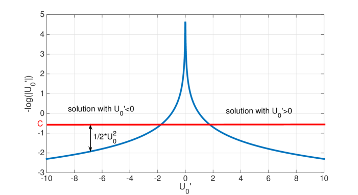
Figure 1: Newtonian structure of the mean flow dynamics. The stationary zonal flow satisfies a Newtonian equation similarly to a particle in a potential. Whatever the value of the integration constant $C$, two classes of solutions exist: one profile has an increasing velocity, the other one has a decreasing velocity.

Whatever the value of the constant $C$, the velocity profile $U_{0}$ always diverges. The derivative $U_{0}^{\prime}$ cannot change sign. There are two classes of solutions, either solutions with $U_{0}^{\prime}>0$ or solutions with $U_{0}^{\prime}<0$. The two classes of solutions correspond to the two sides of a jet. The solution of equation (26) is represented in figure (2). Equation (26) predicts that zonal jets are composed by a succession of diverging velocity profiles, with successively increasing and decreasing values of the velocity. The side of increasing velocity of a jet is totally independent of the side with decreasing velocity. The velocity profiles of westward and eastward jets are symmetric, with in both cases a diverging value of the velocity at the extremum. Such a velocity profile is of course not realistic because the velocity of zonal winds have finite values. By contrast, the qualitative shape of a real profile is displayed by the blue curve in figure (2). Equation (26) predicts the velocity profile in the intermediate regions of monotonic velocity, away from the jet edges.

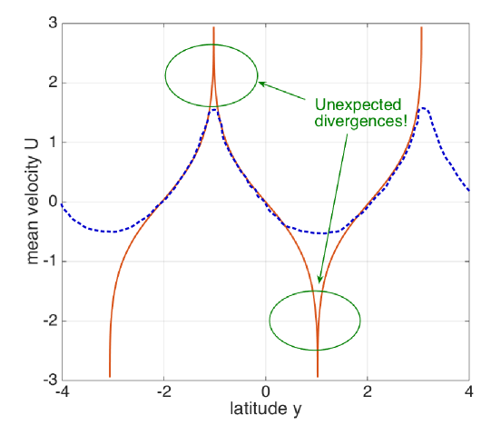
Figure 2: Mean velocity profile in the inertial small scale forcing limit. (Color online) The red curve displays the stationary velocity profile of the zonal flow predicted by equation (26), in the inertial small scale forcing limit. Equation (26) predicts symmetric eastward and westward jets, with diverging values of the velocity at the extrema. The blue curve displays the qualitative shape of a real profile as observed on Jupiter or in numerical simulations (see e.g. figures (3) and (5)). Two different regularization mechanisms prevent the jet divergence in the eastward part and in the westward part respectively.

The fact that equation (26) predicts divergent velocity profiles means that some of the hypotheses leading to the result (23) are broken at the extrema of zonal jets. The asymptotic expansion has been obtained using two major asumptions: first, the limit $\frac{kU^{\prime}}{U^{\prime\prime}}\rightarrow\infty$ should be satisfied, and second the mean flow should be hydrodynamically stable (no unstable modes in equation (18)). The first assumption is broken at the eastward extrema of jets, and the second is broken at the westward extrema. Section 4 explains the regularization mechanism that creates a cusp at the eastward extremum, and section 5.3 shows that an hydrodynamic instability stops the growth of the westward jet at the maximal curvature $\beta$. By taking those physical mechanisms into account, it is possible to get realistic jets that correspond to the observations on Jupiter’s troposphere. The width of jets is not constrained by equation (25). The typical width of a jet is set by the limit curvature $\beta$ at the westward extremum that imposes a minimal spacing between two consecutive jets.

3.4 Interpretation of eq.(23) from the energy balance

We now give a very enlightening interpretation of the result (23) in terms of the energy balance. Multiplying both sides of equation (7), we obtain the energy balance equation for the large scales of the flow

$$\partial_{t}\left(\frac{1}{2}U^{2}\right)+\partial_{y}\left(U\left\langle uv\right\rangle\right)=U^{\prime}\left\langle uv\right\rangle-rU^{2}.$$ (27)

We interpret the different terms in equation (27). $\frac{1}{2}U^{2}$ is the kinetic energy density. The term $\partial_{y}\left(U\left\langle uv\right\rangle\right)$ is a divergence, and thus the quantity $U\left\langle uv\right\rangle$ can be interpreted as the spatial energy flux at large scales. Energy is dissipated by the term $-rU^{2}$. Finally, the term $U^{\prime}\left\langle uv\right\rangle$ can be interpreted as the energy injection rate in the zonal component of the flow. On the other hand, equation (23) can be written as

$$U^{\prime}\left\langle uv\right\rangle=\epsilon$$ (28)

after integration over $y$. From the energy balance (27), the term $U^{\prime}\left\langle uv\right\rangle$ can be interpreted as the rate of energy transferred from the small-scale eddies to the mean flow. $\epsilon$ is the total energy injection rate. Relation (28) thus means that all energy injected at small scale is transferred locally to the largest scale of the flow. The fact that all energy is transferred to the largest svale before being dissipated can be explained by the limits $\alpha\rightarrow 0$ and $K\rightarrow+\infty$. The inertial limit $\alpha\rightarrow 0$ corresponds to a vanishing value of the friction coefficient $r$. In the limit of vanishing friction, the system has no time to dissipate energy at small scale and all energy is transferred to the largest scale. The small scale forcing limit $K\rightarrow+\infty$ prevents energy transfers between the different parts of the flow. The velocity fluctuations at latitude $y$ only interact with the flow in a small region of size of order $\frac{1}{K}$ around. Thus, spatial energy transfer is impossible and energy has to be transferred to the mean flow at the same latitude $y$. For the local velocity fluctuations, the mean flow at scale $\frac{1}{K}$ looks like a parabolic profile with derivative $U^{\prime}(y)$ and second derivative $U^{\prime\prime}(y)$, that’s why the asymptotic development of the Reynolds stress divergence is expressed in terms of $U^{\prime}$ and $U^{\prime\prime}$.

To sum up this idea, we can say that the energy transfer is local in physical space, but nonlocal in Fourier space. Energy is transferred directly from the scale $\frac{1}{K}$ to the mean flow through direct interaction between the mean flow and the eddies, and not through an inverse energy cascade in Fourier space. Energy transfer is possible only if $U^{\prime}\neq 0$. At the extrema of jets, expression (28) breaks because direct energy transfer from small scales to the mean flow is impossible.

4 Cusps for eastward jets

We now assume that there are no hydrodynamical instabilities in the eastward part of zonal jets. In the previous parts of this paper, we saw that the formula (23) $\partial_{y}\left\langle uv\right\rangle=-\epsilon\frac{U^{\prime\prime}}{U^{\prime 2}}$ gives a divergent mean velocity profile and we discussed that this formula can be valid only in the limit $\frac{KU^{\prime}}{U^{\prime\prime}}\rightarrow\infty$. The latter limit is not satisfied close to the eastward extrema. The result (26) shows that the ratio $\frac{KU^{\prime}}{U^{\prime\prime}}$ behaves as $K(y_{cr}-y)$, where $y_{cr}$ is the critical latitude of the eastward divergence. Even for large values of $K$, the asymptotic expansion breaks down in a narrow region of size $\frac{1}{K}$ around the eastward peak. The limit (23) is only valid between the extrema of the jet. But in a region of size $\frac{1}{K}$ around the extremum, another mechanism takes place to stop the jet growth, and regularize the mean velocity profile at scale $\frac{1}{K}$. On Jupiter, the data collected by Gallileo and Cassini probes, displayed in figure (3), indicate that the eastward jets have “cusps”, while westward jets seem smoother. We first discuss eastward jet cusps.

Looking more precisely on the cusp of figure (3), we see that its size is approximately 1 degree i.e a scale of about $1000$ km. When we observe Jupiter’s surface, we can see the fluctuating vortices evolving in a timescale of a few days ((Porco et al., 2003)). The size of those vortices are related to three dimensional motions, producing convection plumes, that develop potential vorticity disturbances at a scale which approximately the Rossby deformation radius of order $1,000\,\mbox{km}$ and with potential vorticity of order $\beta$, the Coriolis parameter. In our effective model of barotropic flows, all these convective phenomena are modeled by the stochastic force. Accordingly, we choose the forcing scale $\frac{1}{K}$ to be of the order of a thousand kilometers.

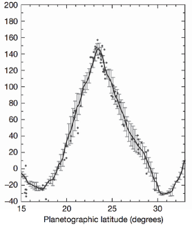
Figure 3: The $24^{o}$N Jupiter eastward jet (taken from (Sánchez-Lavega et al., 2008)). The vertical scale is the mean velocity of the wind ($m.s^{-1}$).

A natural question is: can we have a cusp solution of the stationary equation

$$\left\langle v\omega\right\rangle[U]=U,$$

in the limit $K\rightarrow\infty$?

In order to adress this question, we consider equation (18) and study its large $K$ asymptotic after changing the scale $y\leftarrow Ky$. We denote $\theta$ the angle defined through the relation $\cos\theta:=\frac{k}{K}$. As we are looking for a cusp of size $\frac{1}{K}$, it will be convenient to set $\tilde{U}(y)=U\left(\frac{y}{K}\right)$. This implies that $\frac{1}{K^{2}}U^{\prime\prime}\left(\frac{y}{K}\right)=\tilde{U}"(y)$. Equation (18) becomes

$$\left(\frac{d^{2}}{dy^{2}}-\cos^{2}\theta\right)\varphi_{\epsilon}(y/K,c)+\frac{\beta/K^{2}-\tilde{U}"(y)}{\tilde{U}(y)-c-i\epsilon}\varphi_{\epsilon}(y/K,c)=\frac{\omega(y/K,0)}{ikK^{2}(\tilde{U}(y)-c-i\epsilon)}.$$

We set $ikK^{2}\varphi(y/K,c):=\phi(y,c)$. From (19) the function $\omega^{\infty}$ satisfies

$$\omega^{\infty}\left(\frac{y}{K}\right)=\omega\left(\frac{y}{K},0\right)+\left(\tilde{U}"(y)-\frac{\beta}{K^{2}}\right)\phi_{+}(y,c).$$ (29)

Expression (29) shows that the limit of large $K$ completely cancels the effect of the parameter $\beta$. However the solution $\tilde{U}$ still depends on $\theta$. We first consider the case where the spectrum has only one component $\theta$ . Let $w_{\theta}(y):=\omega^{\infty}\left(\frac{y}{K}\right)$ . Equations (18),(19) and (16) give the set of equations defining the Reynolds stress divergence $\left\langle v\omega\right\rangle[\tilde{U]}$ in the large $K$ limit

$$\left(\frac{d^{2}}{dy^{2}}-\tan^{2}\theta\right)\phi_{\epsilon}(y,c)-\frac{\tilde{U}"(y)}{\tilde{U}(y)-c-i\epsilon}\phi_{\epsilon}(y,c) = \frac{e^{i\sin\theta y}}{\tilde{U}(y)-c-i\epsilon}$$

$$e^{i\sin\theta y}+\tilde{U}"(y)\phi_{+}(y,\tilde{U}(y)) = w_{\theta}(y)$$

$$\frac{1}{\tilde{U}"(y)}[|w_{\theta}(y)|^{2}-1] = \left\langle v\omega\right\rangle_{\theta}[\tilde{U]}.$$ (30)

The first equation is the inhomogenous Rayleigh equation without $\beta$ effect. The second one is the modified expression to compute $\omega^{\infty}$, and the last one is the pseudomomentum balance giving access to the Reynolds stress divergence.

Before we go on with numerical analysis, let us give some analytic results on the set of equations (30).

• We have already given expression (22) for the Reynolds stress divergence in the limit $K\rightarrow+\infty$, away from the extremum of the jet. As we have used the scaling $y\leftarrow Ky$ to find (30), we expect to recover the asymptotic (22) in the limit $y\rightarrow\infty$. For a given profile $\tilde{U}$, we have the asymptotic result $\left\langle v\omega\right\rangle[\tilde{U}]\underset{y\rightarrow\infty}{\sim}-\frac{\tilde{U}"}{\tilde{U}^{\prime 2}}.$

• We know that the relation $\omega^{\infty}(y_{cr})=0$ holds at the extremum (see subsection 3.1), which corresponds here to $w_{\theta}(y_{cr})=0$. At the extremum, the third equality in (30) shows that $\left\langle v\omega\right\rangle=-\frac{1}{\tilde{U}"}$. At a maximum of $U$ (eastward jet), $\tilde{U}"<0$ and the Reynolds stress divergence thus forces the profile $\tilde{U}$ to grow. The contrary happens at a minimum of $U$: we have $\tilde{U}">0$ and the velocity decays, such that its magnitude grows. The consequence is that the turbulence always forces the jet to grow. The growth can be stopped by either linear friction or non linear effects beyond the quasilinear approximation. For westward jets, we will see in section (5.3) that it can also be stopped by an hydrodynamic instability.

• The formula

  $$\left\langle v\omega\right\rangle(y_{cr})=-\frac{1}{\tilde{U}"(y_{cr})}$$ (31)

  is in itself noteworthy. It comes from the phenomenon of depletion of vorticity at the stationary streamlines, which has been already emphasized by (Bouchet & Morita, 2010). To reach the stationary profile, $\left\langle v\omega\right\rangle$ has to equilibrate the linear friction. At the jet extremum, the stationary state of $U$ in (8) gives the equality

  $$\left\langle v\omega\right\rangle(y_{cr})=\tilde{U}(y_{cr}).$$ (32)

  We can thus link the value of the velocity at the extremum of the jet and the curvature of the cusp. Relations (31-32) give the second important result of this paper

  $$\tilde{U}(y_{cr})=-\frac{1}{\tilde{U}^{\prime\prime}(y_{cr})}.$$ (33)

  Coming back to dimensional fields, the eastward cusp satisfies the relation

  $$U(y_{cr})=-\frac{\epsilon K^{2}}{rU^{\prime\prime}(y_{cr})},$$ (34)

  where $\epsilon$ is the energy injection rate. Relation (34) is a universal property of stationary jet profiles. It relates the strength of a jet to its curvature, and the physical parameters $\epsilon,r$ and $K$. It does not depends on the forcing Fourier spectrum, but only on the scale $\frac{1}{K}$ at which energy is injected.
  

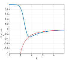
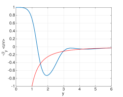
Figure 4: Reynolds stresses close to an eastward jet. Left: the Reynolds stress divergence $-\partial_{y}\left\langle uv\right\rangle$ from (30) for a parabolic profile $\tilde{U}(y)=-\frac{y^{2}}{2}$, and $\theta=\frac{\pi}{8}$. (thick curve). The thin curve depicts the theoretical asymptote $\frac{\tilde{U}"}{\tilde{U}^{\prime 2}}$. As one can notice, $-\partial_{y}\left\langle uv\right\rangle(0)=-\frac{1}{\tilde{U}"}=1$ in agreement with the theoretical result (31). Right: the total Reynolds stress divergence resulting from the sum over $\theta\in\left[-\frac{\pi}{3};\frac{\pi}{3}\right]$. The Reynolds stress divergence has no universal expression in the intermediate region between the cusp (at $y=0$) and the asymptotic region $y\gg 1$. The cusp velocity profile has thus to be computed numerically using the particular shape of the force Fourier spectrum.

Let us illustrate those results by a numerical computation of the nondimensional equations (30). The numerical computation goes the following way: we solve the first equation of (30), for given values of the Laplace transform parameter $\epsilon$ and the phase velocity $c$, and given boundary conditions. We impose vanishing boundary conditions at infinity for $\phi_{\epsilon}$. $\epsilon$ has to be small because we want to compute the solution $\phi_{+}$ when $\epsilon$ goes to zero. The left panel of figure (4) has been obtained with $\epsilon=10^{-5}$. Because the solution $\phi_{+}$ has a singularity at $U(y_{c})=c$, an extreme precision is required to obtain convergence of the numerical calculations. To obtain the value of $\left\langle v\omega\right\rangle_{\theta}(y)$, we have to compute the solution $\phi_{+}$ for $c=\frac{y^{2}}{2}$, and this has to be done for each value of $y$. On the left of figure (4), about 20 values of $y$ were used to plot the blue curve.

The plot of the Reynolds stress divergence in figure (4) clearly displays two regions with a sharp transition (located around $y=2$ in the figure). In the first region, the mean velocity profile forms a cusp, which joins continuously the second region of large $y$ values. The second region corresponds to the domain where the expression $\left\langle v\omega\right\rangle=-\frac{U^{\prime\prime}}{U^{\prime 2}}$ is valid. The velocity profile joining the cusp to the asymptotic profile of figure (2) is non-universal with respect to the forcing spectrum. In the right panel of figure (4), we plot $-\partial_{y}\left\langle uv\right\rangle$ for a uniform forcing spectrum in the range $\theta\in\left[-\frac{\pi}{3};\frac{\pi}{3}\right]$.

With the system of equations (30), we have been able to show that a cusp of typical size $\frac{1}{K}$ forms at the eastward extremum of the jet. This cusp regularizes the velocity profile at its maximum and stops the divergence observed in figure (2). The relation between the curvature of the jet at the extremum and its maximal velocity (34) is universal as it does not involve the explicit expression of the spectrum of the stochastic force. However, the exact velocity profile joining the cusp to the asymptotic profile of figure (2) is rather complicated and is not at all universal.

5 Computation of Reynolds stress divergence for westward jets

As explained in section 4, the parameter $\beta$ disappears from the equations when we try to compute the equilibrium profile in the small scale forcing limit $K\rightarrow\infty$, because the $\beta$ effect becomes irrelevant at the scale $\frac{1}{K}$. Using this approach, we could expect the jet to be symmetric with respect to the transformation $U\rightarrow-U$. At a formal level, nothing in equations (24) nor (30) seems to make any difference between the eastward and the westward part of a jet. However, a look at the jets observed on Jupiter shows a clear asymmetry between eastward and westward jets, especially at high latitudes. One key point is that, as clearly stated, the previous sections assume that the linearized equations close to the jet are stable, and do not sustain neutral modes.

On Jupiter’s jets, cusps only exist on the eastward part whereas the westward part looks like a parabolic profile with curvature between $2\beta$ and $3\beta$ (see figure (5) and (Ingersoll et al., 1981) for a discussion on the value of the curvature). Numerical simulations of the barotropic model also show this asymmetry. In (Constantinou, 2015) for example, the curvature at the eastward jet is almost exactly $\beta$ and seems to be trapped at this value whatever large the coefficients $K$ and $\frac{1}{\alpha}$ are. The value of $\beta-U^{\prime\prime}$ is always positive, and the Rayleigh-Kuo criterion for jet stability is satisfied. The aim of this section is to understand what is the behavior of a parabolic jet with $U^{\prime\prime}$ close to $\beta$ and see if the profile $\beta\frac{y^{2}}{2}$ can or not be a stationary solution of the barotropic model (4).

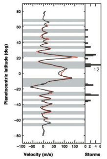
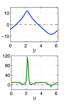
Figure 5: Left panel: zonal jets on Jupiter. Data collected by the Gallileo and Cassini probes (from (Porco et al., 2003)). Right panel: A numerical simulation of the quasilinear barotropic equations (S3T system) performed in (Constantinou, 2015).The top figure displays the mean velocity profile $U$ and the bottom figure displays $\beta-U^{\prime\prime}$. The cusp is obvious on both figures, the peak on the bottom figure corresponds to the eastward extremum of the jet. $\beta-U^{\prime\prime}$ is always positive, thus satisfying the Rayleigh-Kuo criterion except possibly at the westward extremum.

5.1 Modified Rossby waves

We consider in equation (18) a parabolic profile $U(y)=\gamma\frac{y^{2}}{2}$, and we want to study the behavior of the Reynolds stress divergence when $\gamma$ is close to $\beta$. For $\gamma=\beta$, any perturbation is carried freely by the mean flow, and equation (15) reduces to

$$\partial_{t}\omega+ikU\omega=0,$$

which is easily solved by $\omega(y,t)=\omega(y,0)e^{-ikUt}$. Expression (16) is then singular, because $U^{\prime\prime}-\beta$ vanishes in the denominator, and $|\omega^{\infty}|^{2}-1=|\omega(y,0)|^{2}-1=0.$ If we try to compute directly the Reynolds stress divergence $\left\langle v\omega\right\rangle$, we will find a singularity in $y=0$. Therefore, the aim is to compute $\left\langle v\omega\right\rangle$ for $\gamma$ smaller and larger than $\beta$ and let then $\gamma\rightarrow\beta$.

It has been proved long ago that for $0<\gamma<\beta$ we have modified Rossby waves in the flow (Drazin et al., 1982), with at least one Rossby wave as soon as $\gamma<\beta$. In (Brunet, 1990), the case of a parabolic profile is thoroughly studied and a method is found to compute the Rossby waves and their velocity. Basically, it consists in doing a Fourier transform in $y$ and transform the Rayleigh equation into a one dimensional Schrödinger equation. The one dimensional Schrödinger equation describes a particle in a potential vanishing at infinity. Possible bound states of the Schrödinger equation correspond to modified Rosby waves.

For $\gamma>\beta$, the Schrödinger equation potential is positive, and classical results prove that there is no bound state, and thus there is no Rossby waves. In that case expression (16) will be valid to compute the Reynolds stress divergence. By contrast, for $0<\gamma<\beta$, the Schödinger equation potential is negative (the position zero is attractive). Classical results (Reed & Simon, 1978) shows that there exists a least one bound state. There is thus at least one modified Rossby wave. Moreover as the potential deepens for decreasing $\gamma/\beta$, the number of bound states and thus the number of modified Rossby waves increases when $\gamma/\beta$ decreases. When $0<\gamma<\beta,$ because of the presence of waves, we have to use expression (17) to compute the Reynolds stress divergence.

We discuss more precisely the existence of Rossby waves and their computation for a parabolic profile in appendix C.

5.2 Singularity of the Reynolds stress for a jet curvature close to $\beta$

We now compute the Reynolds stress divergence $\left\langle v\omega\right\rangle$ using the same method as for the cusp case discussed in section 4, but without taking the limit $K\rightarrow\infty$. It happens that the parabolic profile has an additional symmetry, it is invariant under the transformation $y\leftarrow Ky$. For a parabolic profile, equation (18) only depends on the parameter $\tan\theta:=\frac{l}{k}$ and $\mu:=1-\frac{\beta}{\gamma}$. As discussed previously, Rossby waves appear when $\mu<0$ (equivalently for $0<\gamma<\beta$).

Using equations (18),(19) and (17), the self-consistent equations for the jet write

$$\left(\frac{d^{2}}{dy^{2}}-\tan^{2}\theta\right)\varphi_{\epsilon}(y,c)-\frac{\mu}{\frac{y^{2}}{2}-c-i\epsilon}\varphi_{\epsilon}(y,c) = \frac{\mathcal{P}e^{i\sin\theta y}}{\frac{y^{2}}{2}-c-i\epsilon}$$

$$\mathcal{P}e^{i\sin\theta y}+\mu\varphi_{+}\left(y,\frac{y^{2}}{2}\right) = w_{\theta}(y)$$

$$\frac{1}{\mu}\left[\left|\left(1-\mathcal{P}\right)e^{i\sin\theta y}\right|^{2}+\left|w_{\theta}(y)\right|^{2}-1\right] = \frac{1}{\gamma}\left\langle v\omega\right\rangle_{\theta}[\tilde{U]}.$$ (35)

We have denoted by $\mathcal{P}$ the projector on the space orthogonal to the neutral modes.

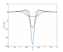
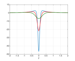
Figure 6: Reynolds stresses close to a westward jet. Left: Minus the Reynolds stress divergence $<v\omega>$ obtained for $\mu=0.3$ (green), $\mu=0.1$ (red) and $\mu=0.05$ (blue). When the parameter $\mu$ comes closer to zero, the divergence at $y=0$ becomes more and more pronounced. Right: Minus the Reynolds stress divergence for $\mu=-0.3$ (green), $\mu=-0.1$ (red) and $\mu=-0.05$ (blue). Other parameters are $\theta=\frac{\pi}{8}$ and $\beta=1$.

The result of the numerical integration of (35) is shown in figure (6). The main result is that the stress $\left\langle v\omega\right\rangle$ has the same qualitative behavior both for $\gamma<\beta$ and for $\gamma>\beta$. For $\gamma>\beta$, i.e $\mu>0$, we still have the result that $w_{\theta}(0)=0$, which implies that the stress $\left\langle v\omega\right\rangle$ is diverging as $-\frac{1}{\mu}$ when $\mu\rightarrow 0^{+}$. For $0<\gamma<\beta$, i.e $\mu<0$, the stress is diverging as $\frac{[|\omega_{\theta}^{1}(0)|^{2}-1]}{\mu}$ when $\mu\rightarrow 0^{-}$. $\omega_{\theta}^{1}$ is the projection of $e^{i\sin y}$ on the first neutral mode. It happens that $|\omega_{\theta}^{1}(0)|^{2}-1$ is always positive. Hence, $\frac{[|\omega_{\theta}^{1}(0)|^{2}-1]}{\mu}$ is negative. We conclude that whatever the sign of $\mu$, the stress $\left\langle v\omega\right\rangle$ has a negative divergence at the minimum of the jet that makes the jet grow.

If the curvature $\gamma$ is smaller than $\beta$, the effect of the Reynolds stress divergence is to narrow the jet and increase the curvature. When $\gamma$ becomes larger than $\beta$, the quasilinear theory predicts that the jet should continue its growth, and form a cusp exactly the same way as for the eastward jet. No mechanism in the quasilinear dynamics can stop the growth of the westward jet. To explain the numerical simulations, we thus have to consider other hypothesis than the ones considered so far. Among those, we have assumed there is no hydrodynamic instability in the set of equations (35), i.e a mode with nonzero imaginary part of the velocity. With $\gamma>\beta$ the Rayleigh–Kuo criterion is violated, the stability of a jet is no longer guaranteed. In the last section of this paper, we will study qualitatively the effect of an instability to see whether it can really stop the growth of the westward jet.

5.3 Hydrodynamic instability in the westward jet

An unstable mode is a solution of the homogeneous Rayleigh equation

$$\left(\frac{\partial^{2}}{\partial y^{2}}-k^{2}\right)\psi+\frac{\beta-U^{\prime\prime}}{U-c}\psi=0$$ (36)

with complex phase speed $c$. In particular for unstable modes, the imaginary part satisfies $kc_{i}>0$ and the consequence is the exponential growth of a disturbance $\left|\psi(y,t)\right|\propto e^{kc_{i}t}$. An unstable mode has a contribution to the Reynolds stress divergence. In stationary state, the flow can only sustain unstable modes satisfying $kc_{i}<\alpha$, otherwise the exponential growth of the unstable mode would create a divergence in the Reynolds stress. If the flow sustain unstable modes, we have to modify expression (17) taking into account the presence of unstable modes. We do not report the computation, it is similar to the one developed in appendix A for neutral modes. Please note that by contrast to neutral modes, the real part $c_{r}$ of the (complex) speed $c$ lies within the range of $U$ ((Drazin & Reid, 2004; Drazin et al., 1982)). The contribution of an instability in the Reynolds stress has been already computed in the deterministic case ((Pedlosky, 1982) p 576), and we modify here the classical result to adapt it to the stochastic case.

Let $\omega^{c}(y)$ be the projection of the initial condition $e^{ily}$ on the unstable mode, and $\psi^{c}$ the associated stream function defined by $\left(\frac{\partial^{2}}{\partial y^{2}}-k^{2}\right)\psi^{c}=\omega^{c}$. The projection refers to the scalar product induced by the pseudomomentum conservation law (see appendix A for the discussion). Then the dominant contribution of the unstable mode in the computation of $2\alpha\left\langle|\omega|^{2}\right\rangle$ writes

$$2\alpha\left\langle|\omega|^{2}\right\rangle = 2\alpha\int_{-\infty}^{0}{\rm d}t~{}e^{2\alpha t}\left|\omega^{c}(y)e^{ikct}\right|^{2}$$ (37)

$$= |\omega^{c}(y)|^{2}\frac{2\alpha}{2\alpha-2kc_{i}}.$$ (38)

Equation (36) shows that

$$\omega^{c}=-\frac{\beta-U^{\prime\prime}}{U-c}\psi^{c}.$$

Equations (38) and (5.3) give the main contribution of an hydrodynamic instability to the Reynolds stress divergence

$$\frac{2\alpha\left\langle|\omega|^{2}\right\rangle}{U^{\prime\prime}-\beta}=-\frac{2\alpha}{2\alpha-2kc_{i}}\frac{|\psi^{c}|^{2}}{|U-c|^{2}}(\beta-U^{\prime\prime}).$$ (39)

Let us emphasize once more that this term is a contribution to the Reynolds stress adding to the other terms coming from the effect of neutral modes and from $\omega^{\infty}$. The important point in (39) is that the coefficient $\frac{2\alpha}{2\alpha-2kc_{i}}\frac{|\psi^{c}|^{2}}{|U-c|^{2}}$ is strictly positive, which means that the term coming from the unstable mode opposes a change of sign of $\beta-U^{\prime\prime}$. In order to equilibrate, the jet needs to make a continuous barotropic adjustment of the mean flow curvature at the westward edge.

In order to illustrate this assertion, we consider a configuration where the instability develops. We perform a direct numerical integration of the equation

$$\partial_{t}\omega+ikU\omega+ik(\beta-U^{\prime\prime})\psi=0,$$

using periodic boundary conditions in $y$ and the initial condition $\omega(y,0)=e^{ily}$. We use a Runge-Kutta algorithm of order 4. The profile $U$ is parabolic with $0<\gamma<\beta$ but we add a small disturbance at the extremum in 0 of the form of a gaussian $-\eta e^{-\frac{y^{2}}{\sigma^{2}}}$. The disturbance mimics qualitatively the effect of the forcing described in figure (6), it models the fact that the mean velocity profile has a narrow curvature at its extremum.

$$U(y)=\gamma\frac{y^{2}}{2}-\eta e^{-\frac{y^{2}}{\sigma^{2}}}.$$ (40)

The values of the chosen parameters are $\beta=1$, $\mu=1-\frac{\beta}{\gamma}=-0.3$, $k=l=10$. $\sigma$ quantifies the width of the disturbance, we chose $\sigma=0.1$. $\eta$ describes the magnitude of the disturbance and is the control parameter of the simulation. Results are displayed in figure (7). The red curve is the graph of $\beta-U^{\prime\prime}(y)$. When this quantity is strictly positive everywhere in the flow, the Rayleigh-Kuo criterion is satisfied and the flow is stable. With the velocity profile chosen in (40), the Rayleigh-Kuo criterion is violated around $y=0$ as displayed by the red curve in figure (7). The blue curve displays the quantity $|\omega|^{2}(y,t)-1$ at $T=30$. In our simulations, we clearly see the three peaks of the blue curve growing exponentially with time, which indicates the existence of an hydrodynamic instability. From left to right, we have increased the value of the parameter $\eta$. The larger $\eta$, the more the Rayleigh-Kuo criterion is violated, and the faster the instability grows. It has been already emphasized that $|\omega|^{2}-1$ has to vanish at the same time where $\beta-U^{\prime\prime}=0$ in the flow, and this is confirmed by our simulation and displayed in figure (7). The largest peak of the blue curve corresponds exactly to the region in the flow where $\beta-U^{\prime\prime}$ is negative.

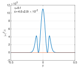
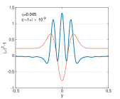
Figure 7: Instability growth for a perturbation of an unstable westward jet. We show here the tensor $|\omega|^{2}-1$ at $T=30$ for different values of $\eta$, and we compute the value of $c$ whenever possible. The thiner curve (red color online) shows $\beta-U^{\prime\prime}$. Close to the instability threshold, it is no longer possible to determine the value of $c$ because the instability growth rate is too slow.

To obtain the mode $\omega^{c}(y)$, we simply look at the convergence of $\omega(y,t)e^{ikct}$. The real and imaginary parts of the unstable mode $\omega^{c}(y)$ are displayed in the left panel of figure (8) in respectively blue and red. The curve $\beta-U^{\prime\prime}$ has been superimposed in yellow. We see again that the unstable mode is vanishing at points where $\beta-U^{\prime\prime}=0$ and that the mode is larger in the region where $\beta-U^{\prime\prime}<0$. In the right panel of figure (8) we display the Reynolds stress divergence $\left\langle v\omega\right\rangle=\frac{|\omega|^{2}-1}{U^{\prime\prime}-\beta}$ obtained from equation (16) with one single Fourier component. As can be checked directly in figure (8) right, the effect of the instability is exactly the opposite as the one in figure (6). The Reynolds stress divergence is positive in the region where the Rayleigh-Kuo criterion is violated, and thus the tensor in figure (8) reequilibrates the profile $U$ and damps the perturbation $-\eta e^{-\frac{y^{2}}{\sigma^{2}}}$.

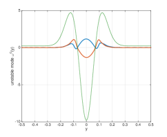
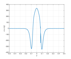
Figure 8: Unstable mode at the westward jet edge. Left: real part (blue curve) and imaginary part (red curve) of the unstable mode $\omega^{c}$. The value of $\eta$ is $0.05$. The thiner curve (green) displays $\beta-U^{\prime\prime}(y)$, the Rayleigh-Kuo criterion is violated in the vincinity of zero. Right: The tensor $\frac{|\omega|^{2}-1}{U^{\prime\prime}-\beta}$ that contributes to the Reynolds stress divergence obtained for T=30. The artefact comes from the fact that $U^{\prime\prime}-\beta$ vanishes and that we use a finite discretisation in $y$. The effect of this tensor is to reequilibrate the velocity $U$ to satisfy $\beta-U^{\prime\prime}>0$. The value of $c$ is $c=-2.02+1.04i~{}e-2$

Let us summarize the results of the present section. We have first investigated the behavior of the Reynolds stress divergence for a parabolic profile, because numerical simulations show that the mean velocity profile is almost parabolic for westward jets. The Reynolds stress divergence is the tensor that forces the mean flow according to equation (7). Even if we cannot always compute exactly this tensor, we can study its sign and its qualitative properties to see whether it damps the flow or not. We first did the assumption that there is no hydrodynamic instability in the flow. This assumption leads to a contradiction for the parabolic profile because the Reynolds stress divergence distorts the parabolic profile at $y=0$ as shown in figure (6). Thus, we conclude that another mechanism takes place to equilibrate the parabolic profile. When we consider a small violation of the Rayleigh-Kuo criterion near $y=0$, we see numerically the growth of an instability that opposes exactly to the distortion of the parabolic profile where the Rayleigh-Kuo criterion is violated. Those results are qualitative, we did not compute the equilibrium velocity profile. But it is consistent to assume that the equilibration mechanism is a kind of barotropic adjustment of the mean flow: an instability develops as soon as $\beta-U^{\prime\prime}$ changes sign. The flow has to adjust itself such that the instability is not too large, i.e close to a parabolic profile with $U^{\prime\prime}\sim\beta$, and such that the instability can be damped by linear friction.

6 Conclusion and perpectives

The stochastic barotropic $\beta$ plane model is the simplest model in the hierarchy of models aiming at understanding jet formation in atmosphere dynamics. The precise structure of jets in this simple and fundamental model is still not really understood beyond qualitative description and orders of magnitude estimates, although thousands of papers have been written on the subject. In this paper we have proposed three main contributions to the theoretical understanding of these zonal jets to make progresses in this direction. Our analytical results are valid when assuming both the inertial and the small scale forcing limits. The inertial limit is valid when the timescales related to the inviscid dynamics (perfect transport, shearing and mixing, Rossby waves, and so on) are much smaller than the timescale for spin up and spin down (related to forcing and dissipation). In the the stochastic barotropic model, this is quantified by a small value of the nondimensional parameter $\alpha=L\sqrt{r^{3}/\epsilon}$ . The limit of small scale forces is relevant when the typical scale for the forcing, $1/K$, is much smaller than the typical jet width, of the order of the Rhines scale. Those two limits are relavant for instance for the largest zonal jets of Jupiter.

With these two limits, the interaction between the large scale zonal jets and the small scale turbulence becomes local in physical space. The energy is transferred directly from its injection scale to the zonal jet through the direct interaction between the jet and turbulence. Our first contribution has been to justify the local formula $\left\langle uv\right\rangle=\frac{\epsilon}{U^{\prime}}$. This formula could have been obtained directly taking the limit of small friction in the formula of (Srinivasan & Young, 2014), or by neglecting the nonlinear and pressure terms in the energy balance as done by (Laurie et al., 2014) for the case of 2D turbulence. Our justification is based on the double limit discussed in the previous paragraph. The mathematical difficulty resides in considering the inertial limit before the limit of small scale forces. This order of the limits is necessary if one wants to deal with situations for which the dissipation mechanism is much smaller than the inertial one at the forcing scale, which is the case for most geophysical turbulent flows.

Because jets have non-monotonic velocity profiles, the asymptotic expansion and the formula $\left\langle uv\right\rangle=\frac{\epsilon}{U^{\prime}}$ break down at the jet edges where $U^{\prime}=0$. The first naive computation of the velocity profile in the limit $K\rightarrow\infty$ leads to a divergence of the velocity at the extremum, and confirms that the dynamics may lead to several velocity sign reversal. For the asymptotic expansion to be valid, the parameter $\frac{KU^{\prime}}{U^{\prime\prime}}$ has to be large. At the eastward jet edges, we have established that the velocity profile is regularized by a cusp at a typical scale of $1/K$. In the inertial limit $\alpha\rightarrow 0$, we have derived a system of equations that describes the cusp velocity profile. The resulting shape depends on the forcing spectrum. Nevertheless, the mechanism of depletion of vorticity at the stationary streamlines leads to an interesting relation between the curvature of the cusp and the maximal velocity (34), $U(y_{cr})U^{\prime\prime}(y_{cr})=-\epsilon K^{2}/r$, which does not depend on the force spectrum but just on the energy injection rate $\epsilon$.

As observed in previous numerical studies of the barotropic model, the westward jet edges have a curvature $U^{\prime\prime}$ of order $\beta$ in the inertial limit. Based on observations in numerical studies, the mechanism of barotropic adjustment has been discussed for this selection of the jet curvature (see for instance (Constantinou et al., 2012)). In the present work we have for the first time derived and analyzed the equations that describe the westward jet edges in the inertial limit. This theoretical analysis confirms the mechanism of barotropic adjustment. Bellow the stability threshold, the Reynolds stress divergence forces the mean flow to grow. But as soon as the mean flow has a curvature $U^{\prime\prime}>\beta$, an hydrodynamic instability opposes the growth of the velocity profile. Therefore, the parabolic profile is stabilized with a curvature fluctuating close to $\beta$. The flow remains close to marginal stability.

Our work gives an overall picture of the equilibration mechanism and the stationary velocity profile of barotropic zonal jets. Our work can be considered as a theoretical derivation that the jet velocity profile is close to the "PV staircase" in the inertial and small scale forcing limit. The "PV staircase" idea is closely related to the qualitative ideas of homogenization of potential vorticity first proposed by Rhines and Young, and can be justified qualitatively by equilibrium statistical mechanics. However those qualitative ideas do not allow for clear predictions. In the context of barotropic jets and Jupiter jets, The "PV staircase" empirical evidence or the "PV staircase" assumption were discussed thoroughly by (Dritschel & McIntyre, 2008). For instance, (Dritschel & McIntyre, 2008) showed that the "PV staircase" assumption allows to derive straightforwardly the number and the size of jets in a flow configuration. One should bear in mind that the "stairs" are an idealization of the real profile: the discontinuity in the staircase profile corresponds to the cusp at the eastward extremum. It has thus a finite width typically given by $\frac{1}{K}$, where K is the typical wavevector of small-scale energy injection. Besides, the "stairs" are not perfectly flat, because the curvature of the jet is close to $\beta$ at the westward extremum, but not between the extrema. In the monotonic region between the extrema, the mean velocity profile is described by equation (3.9). The "PV staircase" profile can thus be seen as a very good approximation, our theoretical approach gives a more precise mathematical description of the actual profile which is valid within the asymptotic regime of inertial and small scale forcing limit. Moreover, a given flow can sustain different numbers of jets (Bakas & Ioannou, 2013; Constantinou et al., 2012) for the same value of the parameter. This observation cannot be predicted neither from the "PV staircase" approximation, nor from the results we presented in this work. Complementing this work results in order to determine the correct number and spacing between those jets is a challenging problem that might be addressed in the future.

Westward jets on Jupiter display a parabolic profile, but with a curvature $U^{\prime\prime}$ clearly larger than $\beta$. This is one reason why the barotropic model is not sufficient to describe Jupiter’s atmosphere. We believe our analysis could be extended to more refined models, for example a two-layer model. The generalization of our analytical results for a two-layer quasi-geostrophic model would be a very interesting extension of this work. Another natural extension would be the study of rare transitions between states with a different number of jets, within the theoretical framework discussed in this paper.

Appendix A The Reynolds stress divergence in the inertial limit

The aim of this section is to give the proof of formula (16) and (17). We have to compute

$$2\alpha\left\langle|\omega|^{2}\right\rangle=2\alpha\int_{-\infty}^{0}{\rm d}t~{}e^{2\alpha t}\left|e^{tL_{k}}[c_{l}]\right|^{2},$$ (41)

where $e^{tL_{k}}[c_{l}]:=\omega_{d}$ is the solution to the deterministic equation

$$\partial_{t}\omega_{d}+ikU\omega_{d}+ik(\beta-U^{\prime\prime})\psi_{d} = 0$$ (42)

$$\left(\partial_{y}^{2}-k^{2}\right)\psi_{d} = \omega_{d}$$

with initial condition $c_{l}(y)=e^{ily}$. We will first assume there are no neutral modes solutions of (42). First, we do the change of timescale $2\alpha t\rightarrow t$ in the integral of (41). It gives us

$$2\alpha\left\langle|\omega|^{2}\right\rangle=\int_{-\infty}^{0}{\rm d}t~{}e^{t}\left|e^{\frac{t}{2\alpha}L_{k}}[c_{l}]\right|^{2}.$$

When $\alpha$ goes to zero, the term $e^{\frac{t}{2\alpha}L_{k}}[c_{l}]$ is the long time limit of the solution of (42). We use the nontrivial result for the case of non monotonous flows, of (Bouchet & Morita, 2010) already mentioned, that there exists a function $\omega_{d}^{\infty}(y)$ such that $\omega_{d}(y,t)\underset{t\rightarrow\infty}{\sim}\omega_{d}^{\infty}(y)e^{-ikUt}$ when there are no neutral modes. Hence $\left|e^{\frac{t}{2\alpha}L_{k}}[c_{l}]\right|\rightarrow|\omega_{d}^{\infty}(y)|$ , and the presence of the exponential in the integral ensures the convergence of the whole. This proves that without neutral modes

$$2\alpha\left\langle|\omega|^{2}\right\rangle\underset{\alpha\rightarrow 0}{\longrightarrow}|\omega_{d}^{\infty}|^{2}.$$

The second case, with neutral modes, is a bit more subtle. The result of (Bouchet & Morita, 2010) relies on a Laplace transform of $\omega_{d}$ denoted $\hat{\omega}_{d}$. To do the inverse Laplace transform, one has to know where the singularities of $\hat{\omega_{d}}$ are. The presence of modes in the equation is exactly equivalent to the presence of poles of order 1 in the complex plane for $\hat{\omega}_{d}$. For unstable modes, these poles have an imaginary part, whereas for neutral modes, they are located on the real axis. We also assume in our calculation that there are no instabilities, which means that all singularities of $\hat{\omega}_{d}$ are on the real axis. Some of these singularities are outside the range of $U$ (outside of [$U_{min},U_{max}$]) and are isolated, they correspond to neutral modes or “modified Rossby waves”. But there is also a continuum of singularities all along the range of U. The integration around the isolated singularities will give the contribution of neutral modes, and it is of the form $\underset{a}{\sum}\omega^{a}(y)e^{ikc_{a}t}$ where $a$ is the mode index, $c_{a}$ is the mode frequency, and the $\omega^{a}(y)$ are the projections of the initial condition $c_{l}$ on the modes $\zeta^{a}(y)$. The projections are defined with the natural scalar product induced by the pseudomomentum conservation law, that is $\ll\omega_{1}^{*}\omega_{2}\gg=\int\frac{\omega_{1}^{*}\omega_{2}}{U^{\prime\prime}-\beta}{\rm d}y$. For this particular scalar product, the operator $\omega\rightarrow U\omega+(\beta-U^{\prime\prime})\psi$ is self-adjoint, and this implies that its eigenvectors are orthogonal with respect to this scalar product. We substract the contribution of the modes $\zeta^{a}(y)$ from the initial condition $c_{l}$, that is, we use $c_{l}-\underset{a}{\sum}\omega^{a}$ as initial condition in (42). We are left with the continuum part of the singularities and the result of (Bouchet & Morita, 2010) holds. As a consequence, there exists a function $\tilde{\omega}_{d}^{\infty}(y)$ such that the remaining part of the solution behaves at infinity like $\tilde{\omega}_{d}^{\infty}(y)e^{-ikU(y)t}.$ We eventually find that for long time, the solution of the deterministic equation behaves like

$$\omega_{d}(y,t)\underset{t\rightarrow\infty}{\sim}\underset{a}{\sum}\omega^{a}(y)e^{-ikc_{a}t}+\tilde{\omega}_{d}^{\infty}(y)e^{-ikU(y)t}.$$

When we inject this result in the expression of $\left|e^{\frac{t}{\alpha}L_{k}}[e_{l}]\right|^{2}$ we get three different terms.

1. Terms coming from the mode-mode contribution of the form $\underset{a}{\sum}|\omega^{a}(y)|^{2}$. The time integration is then trivial.

2. The term coming from the continuum gives us immediately the contribution $|\tilde{\omega}_{d}^{\infty}(y)|^{2}$.

3. What happens for terms of the form $\omega^{a*}\tilde{\omega}^{\infty}e^{-ik(U-c_{a})\frac{t}{\alpha}}$ and $\omega^{a*}\omega^{b}e^{-ik(c_{b}-c_{a})\frac{t}{\alpha}}$ ? The frequencies $\frac{1}{\alpha}k(U-c_{a})$ and $\frac{1}{\alpha}k(c_{a}-c_{b})$ grow to infinity as $\alpha$ vanishes. We have an oscillating integral with frequency growing to infinity. It is a well known result that such an integral asymptotically decays. The cross terms gives no contributions.

We have then proved the desired result that

$$2\alpha\left\langle|\omega|^{2}\right\rangle\underset{\alpha\rightarrow 0}{\longrightarrow}\underset{a}{\sum}|\omega^{a}|^{2}+|\tilde{\omega}_{d}^{\infty}|^{2}.$$

Appendix B Computation of the Reynolds stress in the inertial and small scale forcing regime

In this appendix we prove that

$$\mathcal{R}e\left\langle v_{\theta}^{*}\omega_{\theta}\right\rangle\underset{K\rightarrow\infty\alpha\rightarrow 0}{\rightarrow}\frac{U^{\prime\prime}}{U^{\prime 2}}.$$

In section 3, we found the expression

$$\mathcal{R}e\left\langle v_{\theta}^{*}\omega_{\theta}\right\rangle\underset{K\rightarrow\infty}{\sim}-\frac{\hat{C}_{k,l}}{2k^{2}}\mathcal{P}\left\{\int{\rm d}Ye^{-|Y|}\frac{\cos(Y\tan\theta)}{U\left(y-\frac{Y}{k}\right)-U(y)}\right\}.$$

This expression has no meaning for $y_{c}$ such that $U^{\prime}(y_{c})=0$ because we have a quadratic singularity in the integral. We therefore assume that $U^{\prime}(y)$ does not vanish. With this assumption we get

$$\mathcal{P}\left\{\int{\rm d}Ye^{-|Y|}\frac{\cos(Y\tan\theta)}{U\left(y-\frac{Y}{k}\right)-U(y)}\right\} =\underset{\eta\rightarrow 0}{\lim}\int_{-\infty}^{-\eta}{\rm d}Ye^{-|Y|}\frac{\cos(Y\tan\theta)}{U\left(y-\frac{Y}{k}\right)-U(y)}+\int_{\eta}^{+\infty}{\rm d}Ye^{-|Y|}\frac{\cos(Y\tan\theta)}{U\left(y-\frac{Y}{k}\right)-U(y)}$$

$$=\int_{0}^{+\infty}{\rm d}Ye^{-|Y|}\cos(Y\tan\theta)\left\{\frac{1}{U\left(y-\frac{Y}{k}\right)-U(y)}+\frac{1}{U\left(y+\frac{Y}{k}\right)-U(y)}\right\}$$

$$=\int_{0}^{+\infty}{\rm d}Ye^{-|Y|}\cos(Y\tan\theta)\left\{\frac{U\left(y-\frac{Y}{k}\right)+U\left(y+\frac{Y}{k}\right)-2U(y)}{\left(U\left(y-\frac{Y}{k}\right)-U(y)\right)\left(U\left(y+\frac{Y}{k}\right)-U(y)\right)}\right\}$$

$$\underset{k\rightarrow\infty}{\rightarrow}\frac{U^{\prime\prime}}{U^{\prime 2}}\int_{0}^{+\infty}{\rm d}Ye^{-|Y|}\cos(Y\tan\theta)=\frac{U^{\prime\prime}}{U^{\prime 2}}\frac{1}{1+\tan^{2}\theta}.$$

We have used the relations

$$U\left(y-\frac{Y}{k}\right)+U\left(y+\frac{Y}{k}\right)-2U(y)\sim U^{\prime\prime}\frac{Y^{2}}{k^{2}}$$

and

$$\left(U\left(y-\frac{Y}{k}\right)-U(y)\right)\left(U\left(y+\frac{Y}{k}\right)-U(y)\right)\sim U^{\prime 2}\frac{Y^{2}}{k^{2}}.$$

We have thus

$$\mathcal{R}e\left\langle v_{\theta}^{*}\omega_{\theta}\right\rangle\underset{K\rightarrow\infty}{\sim}-\frac{\hat{C}_{k,l}}{2k^{2}}\frac{U^{\prime\prime}}{U^{\prime 2}}\frac{1}{1+\tan^{2}\theta}=-\frac{\hat{C}_{k,l}}{2K^{2}}\frac{U^{\prime\prime}}{U^{\prime 2}}.$$

Finally, we use the power input relation $\frac{1}{2}\iint{\rm d}k^{\prime}{\rm d}l^{\prime}\frac{\hat{C}_{k^{\prime},l^{\prime}}}{K^{\prime 2}}=1$. When we integrate relation (B) over the whole spectrum, we get the desired result (B).

Appendix C Modified Rossby waves

In this appendix, we discuss the neutral modes of parabolic jets $U(y)=\gamma\frac{y^{2}}{2}$. We first note that for any parabolic jet, $U^{\prime\prime}-\beta$ does not change sign. Hence the Rayleigh-Kuo criteria is satisfied and the jet has no unstable modes.

For a mean velocity $U(y)=\gamma\frac{y^{2}}{2}$, we are looking for solutions of (15) of the form $\omega_{k}(y)e^{-ikct}$. The equation writes

$$-ikc\omega_{k}+ik\gamma\frac{y^{2}}{2}\omega_{k}+ik(\beta-\gamma)H_{k}*\omega_{k}=0.$$

We do the Fourier transform $\hat{\omega}_{k}(l):=\int{\rm d}y\omega_{k}(y)e^{-ily}$ to obtain

$$-\frac{1}{2}\frac{{\rm d}^{2}}{{\rm d}l^{2}}\hat{\omega}_{k}+\frac{\mu}{k^{2}+l^{2}}\hat{\omega}_{k}=\frac{c}{\gamma}\hat{\omega}_{k},$$ (43)

where $\mu:=1-\frac{\beta}{\gamma}$. We recognize the eigenvalue problem for a Schrödinger operator for a particle with potential $\frac{\mu}{k^{2}+l^{2}}$, a result already obtained by Brunet (Brunet, 1990). Using classical results for this type of 1D Schrödinger equation, we can immediately conclude that

• There exists a solution $\hat{\omega}_{k}$ in $L_{2}$ iff $\mu<0$ (attractive potential). In that case, the corresponding eigenvalue is negative which implies that $\frac{c}{\gamma}<0.$ The condition $\mu<0$ imposes already $\gamma>0$, so the phase velocity of Rossbywave is $c<0$ and the wave is outside of the continuous spectrum. We find for this particular configuration the classical result that Rossby waves propagate with $c<U_{min}$.

• The number of modes $n\left(\left|\mu\right|\right)$ increases with $\left|\mu\right|$, the depth of the potential well. Modes organize into continuous families $\left\{\Omega_{i}\left(\left|\mu\right|\right)\right\}_{1\leq i\leq n\left(\left|\mu\right|\right)}$, with energies $E_{i}\left(\left|\mu\right|\right)=\frac{c}{\gamma}$, when $\left|\mu\right|$ is changed. $E_{i}\left(\left|\mu\right|\right)$ are decreasing functions of $\left|\mu\right|$. The families $\Omega_{i}$ are alternatively even and odd functions with a number of nodes that increases with $i$. A new set of modes appears for critical values $\mu_{i}$. For $\mu=\mu_{i}$, the mode of the new family has a zero energy $E_{i}\left(\left|\mu_{i}\right|\right)=0$.

To compute the eigenfunction of (43), for a given $\mu$ we use a bisection algorithm. We divide the interval $[\mu,0]$ in sufficiently small intervals $[\tau_{i},\tau_{i+1}]$ and compute the solution of (43) with $\frac{c}{\gamma}=\tau_{i}$. The solution diverges like an exponential at infinity, and when this divergence changes sign between $\tau_{i}$ and $\tau_{i+1}$, it means that we have an eigenfunction in the interval, and we iterate the algorithm until $\tau_{i+1}-\tau_{i}$ is small enough. This way, we obtain the Fourier transform of a mode, we just have to inverse the Fourier transform to get the mode in real space. Then we project $e^{ily}$ on these modes with the standard scalar product on $L_{2}$. Figure (9) displays the 3 first eigenfunctions obtained with $\mu=-1$.

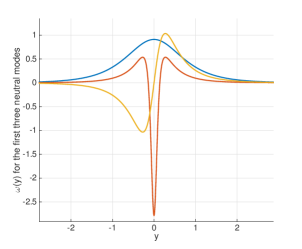
Figure 9: The first three neutral modes (modified Rossby waves) obtained for $\mu=-1$. Even modes and odd modes alternate. The first mode vanishes only at infinity, and each new mode has an additional zero.

References

- Bakas & Ioannou (2013) Bakas, Nikolaos & Ioannou, Petros 2013 A theory for the emergence of coherent structures in beta-plane turbulence. preprint arXiv:1303.6435 .
- Bouchet & Morita (2010) Bouchet, F. & Morita, H. 2010 Large time behavior and asymptotic stability of the 2D Euler and linearized Euler equations. Physica D Nonlinear Phenomena 239, 948–966, arXiv: 0905.1551.
- Bouchet et al. (2013) Bouchet, Freddy, Nardini, Cesare & Tangarife, Tomás 2013 Kinetic theory of jet dynamics in the stochastic barotropic and 2d navier-stokes equations. Journal of Statistical Physics 153 (4), 572–625.
- Bouchet et al. (2016) Bouchet, F, Nardini, C & Tangarife, T 2016 Kinetic theory and quasilinear theories of jet dynamics. arXiv preprint arXiv:1602.02879, to be published in the book Zonal Flows, edited by Boris Galperin, and to be published by Cambridge University Press. .
- Bouchet & Simonnet (2009) Bouchet, F. & Simonnet, E. 2009 Random Changes of Flow Topology in Two-Dimensional and Geophysical Turbulence. Physical Review Letters 102 (9), 094504.
- Bouchet & Venaille (2012) Bouchet, F. & Venaille, A. 2012 Statistical mechanics of two-dimensional and geophysical flows. Physics Reports 515, 227–295.
- Brunet (1990) Brunet, Gilbert 1990 Dynamique des ondes de Rossby dans un jet parabolique.. Universite McGill.
- Constantinou (2015) Constantinou, Navid C 2015 Formation of large-scale structures by turbulence in rotating planets. arXiv preprint arXiv:1503.07644 .
- Constantinou et al. (2012) Constantinou, Navid C, Ioannou, Petros J & Farrell, Brian F 2012 Emergence and equilibration of jets in beta-plane turbulence. arXiv preprint arXiv:1208.5665 .
- Drazin et al. (1982) Drazin, PG, Beaumont, DN & Coaker, SA 1982 On rossby waves modified by basic shear, and barotropic instability. Journal of Fluid Mechanics 124, 439–456.
- Drazin & Reid (2004) Drazin, Philip G & Reid, William Hill 2004 Hydrodynamic stability. Cambridge university press.
- Dritschel & McIntyre (2008) Dritschel, D. G. & McIntyre, M. E. 2008 Multiple Jets as PV Staircases: The Phillips Effect and the Resilience of Eddy-Transport Barriers. Journal of Atmospheric Sciences 65, 855.
- Farrell & Ioannou (2003) Farrell, Brian F. & Ioannou, Petros J. 2003 Structural stability of turbulent jets. Journal of Atmospheric Sciences 60, 2101–2118.
- Farrell & Ioannou (2007) Farrell, B. F. & Ioannou, P. J. 2007 Structure and Spacing of Jets in Barotropic Turbulence. Journal of Atmospheric Sciences 64, 3652.
- Frishman et al. (2017) Frishman, Anna, Laurie, Jason & Falkovich, Gregory 2017 Jets or vortices?what flows are generated by an inverse turbulent cascade? Physical Review Fluids 2 (3), 032602.
- Galperin et al. (2001) Galperin, Boris, Sukoriansky, Semion & Huang, Huei-Ping 2001 Universal n- 5 spectrum of zonal flows on giant planets. Physics of Fluids (1994-present) 13 (6), 1545–1548.
- Galperin et al. (2014) Galperin, Boris, Young, Roland MB, Sukoriansky, Semion, Dikovskaya, Nadejda, Read, Peter L, Lancaster, Andrew J & Armstrong, David 2014 Cassini observations reveal a regime of zonostrophic macroturbulence on jupiter. Icarus 229, 295–320.
- Garcí et al. (2001) Garcí, E, Sánchez-Lavega, A & others 2001 A study of the stability of jovian zonal winds from hst images: 1995–2000. Icarus 152 (2), 316–330.
- Ingersoll (1990) Ingersoll, Andrew P 1990 Atmospheric dynamics of the outer planets. Science 248 (4953), 308–315.
- Ingersoll et al. (1981) Ingersoll, Andrew P, Beebe, Reta F, Mitchell, Jim L, Garneau, Glenn W, Yagi, Gary M & Müller, Jan-Peter 1981 Interaction of eddies and mean zonal flow on jupiter as inferred from voyager 1 and 2 images. Journal of Geophysical Research A 86 (A10), 8733–8743.
- Kolokolov & Lebedev (2016a) Kolokolov, IV & Lebedev, VV 2016a Structure of coherent vortices generated by the inverse cascade of two-dimensional turbulence in a finite box. Physical Review E 93 (3), 033104.
- Kolokolov & Lebedev (2016b) Kolokolov, IV & Lebedev, VV 2016b Velocity statistics inside coherent vortices generated by the inverse cascade of 2-d turbulence. Journal of Fluid Mechanics 809.
- Laurie et al. (2014) Laurie, Jason, Boffetta, Guido, Falkovich, Gregory, Kolokolov, Igor & Lebedev, Vladimir 2014 Universal profile of the vortex condensate in two-dimensional turbulence. Physical review letters 113 (25), 254503.
- Li et al. (2006) Li, Liming, Ingersoll, Andrew P & Huang, Xianglei 2006 Interaction of moist convection with zonal jets on jupiter and saturn. Icarus 180 (1), 113–123.
- Marston et al. (2008) Marston, J. B., Conover, E. & Schneider, T. 2008 Statistics of an Unstable Barotropic Jet from a Cumulant Expansion. Journal of Atmospheric Sciences 65, 1955, arXiv: 0705.0011.
- Pedlosky (1964) Pedlosky, Joseph 1964 The stability of currents in the atmosphere and the ocean: Part ii. Journal of the Atmospheric Sciences 21 (4), 342–353.
- Pedlosky (1982) Pedlosky, J. 1982 Geophysical fluid dynamics. New York and Berlin, Springer-Verlag, 1982. 636 p.
- Porco et al. (2003) Porco, Carolyn C, West, Robert A, McEwen, Alfred, Del Genio, Anthony D, Ingersoll, Andrew P, Thomas, Peter, Squyres, Steve, Dones, Luke, Murray, Carl D, Johnson, Torrence V & others 2003 Cassini imaging of jupiter’s atmosphere, satellites, and rings. Science 299 (5612), 1541–1547.
- Read et al. (2004) Read, PL, Yamazaki, YH, Lewis, SR, Williams, Paul David, Miki-Yamazaki, K, Sommeria, Joël, Didelle, Henri & Fincham, A 2004 Jupiter’s and saturn’s convectively driven banded jets in the laboratory. Geophysical research letters 31 (22).
- Reed & Simon (1978) Reed, Michael & Simon, Barry 1978 Modern methods of mathematical physics. Analysis of Operators, Academic Press .
- Salyk et al. (2006) Salyk, Colette, Ingersoll, Andrew P, Lorre, Jean, Vasavada, Ashwin & Del Genio, Anthony D 2006 Interaction between eddies and mean flow in jupiter’s atmosphere: Analysis of cassini imaging data. Icarus 185 (2), 430–442.
- Sánchez-Lavega et al. (2008) Sánchez-Lavega, A, Orton, GS, Hueso, R, García-Melendo, E, Pérez-Hoyos, S, Simon-Miller, A, Rojas, JF, Gómez, JM, Yanamandra-Fisher, P, Fletcher, L & others 2008 Depth of a strong jovian jet from a planetary-scale disturbance driven by storms. Nature 451 (7177), 437–440.
- Schneider & Liu (2009) Schneider, T. & Liu, J. 2009 Formation of Jets and Equatorial Superrotation on Jupiter. Journal of Atmospheric Sciences 66, 579–+, arXiv: 0809.4302.
- Sommeria (1986) Sommeria, J. 1986 Experimental study of the two-dimensional inverse energy cascade in a square box. Journal of Fluid Mechanics 170, 139–68.
- Srinivasan & Young (2014) Srinivasan, Kaushik & Young, WR 2014 Reynolds stress and eddy diffusivity of -plane shear flows. Journal of the Atmospheric Sciences 71 (6), 2169–2185.
- Vallis & Maltrud (1993) Vallis, Geoffrey K & Maltrud, Matthew E 1993 Generation of mean flows and jets on a beta plane and over topography. Journal of physical oceanography 23 (7), 1346–1362.
- Vasavada & Showman (2005) Vasavada, Ashwin R & Showman, Adam P 2005 Jovian atmospheric dynamics: An update after galileo and cassini. Reports on Progress in Physics 68 (8), 1935.
- Williams (1978) Williams, Gareth P 1978 Planetary circulations: 1. barotropic representation of jovian and terrestrial turbulence. Journal of the Atmospheric Sciences 35 (8), 1399–1426.
- Woillez & Bouchet (2017) Woillez, E & Bouchet, F 2017 Theoretical prediction of reynolds stresses and velocity profiles for barotropic turbulent jets. EPL (Europhysics Letters) 118 (5), 54002.