Transfer Adversarial Hashing for Hamming Space Retrieval
Abstract
Hashing is widely applied to large-scale image retrieval due to the storage and retrieval efficiency. Existing work on deep hashing assumes that the database in the target domain is identically distributed with the training set in the source domain. This paper relaxes this assumption to a transfer retrieval setting, which allows the database and the training set to come from different but relevant domains. However, the transfer retrieval setting will introduce two technical difficulties: first, the hash model trained on the source domain cannot work well on the target domain due to the large distribution gap; second, the domain gap makes it difficult to concentrate the database points to be within a small Hamming ball. As a consequence, transfer retrieval performance within Hamming Radius 2 degrades significantly in existing hashing methods. This paper presents Transfer Adversarial Hashing (TAH), a new hybrid deep architecture that incorporates a pairwise -distribution cross-entropy loss to learn concentrated hash codes and an adversarial network to align the data distributions between the source and target domains. TAH can generate compact transfer hash codes for efficient image retrieval on both source and target domains. Comprehensive experiments validate that TAH yields state of the art Hamming space retrieval performance on standard datasets.
Introduction
With increasing large-scale and high-dimensional image data emerging in search engines and social networks, image retrieval has attracted increasing attention in computer vision community. Approximate nearest neighbors (ANN) search is an important method for image retrieval. Parallel to the traditional indexing methods (?), another advantageous solution is hashing methods (?), which transform high-dimensional image data into compact binary codes and generate similar binary codes for similar data items. In this paper, we will focus on data-dependent hash encoding schemes for efficient image retrieval, which have shown better performance than data-independent hashing methods, e.g. Locality-Sensitive Hashing (LSH) (?).
There are two related search problems in hashing (?), -NN search and Point Location in Equal Balls (PLEB) (?). Given a database of hash codes, -NN search aims to find codes in database that are closest in Hamming distance to a given query. With the Definition that a binary code is an - of a query code if it differs from in bits or less, PLEB for Equal Ball finds all - of a query in the database. This paper will focus on PLEB search which we call Hamming Space Retrieval.
For binary codes of bits, the number of distinct hash buckets to examine is . grows rapidly with and when , it only requires time for each query to find all -. Therefore, the search efficiency and quality within Hamming Radius 2 is an important technical backbone of hashing.
Previous image hashing methods (?; ?; ?; ?; ?; ?; ?; ?; ?; ?; ?; ?; ?; ?; ?; ?; ?; ?; ?; ?) have achieved promising image retrieval performance. However, they all require that the source domain and the target domain are the same, under which they can directly apply the model trained on train images to database images. Many real-world applications actually violate this assumption where source and target domain are different. For example, one person want to build a search engine on real-world images, but unfortunately, he/she only has images rendered from 3D model with known similarity and real-world images without any supervised similarity. Thus, a method for the transfer setting is needed.
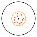
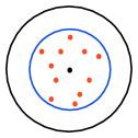
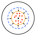
The transfer retrieval setting can raise two problems. The first is that the similar points of a query within its Hamming Radius 2 Ball will deviate more from the query. As shown in Figure 1(a), the red points similar to black query in the orange Hamming Ball (Hamming Radius 2 Ball) of the source domain scatter more sparsely in a blue larger Hamming Ball of the target domain in Figure 1(b), indicating that the number of similar points within Hamming Radius 2 decreases because of the domain gap. This can be validated in Table 1 by the decreasing of average number of similar points of DHN from on task to on task. Thus, we propose a new similarity function based on -distribution and Hamming distance, denoted as -Transfer in Figure 1 and Table 1. From Figure 1(b)-1(c) and Table 1, we can observe that our proposed similarity function can draw similar points closer and let them locate in the Hamming Radius 2 Ball of the query.
| Task | DHN | DHN-Transfer | -Transfer |
| #Similar Points | 1450 | 58 | 620 |
The second problem is that substantial gap across Hamming spaces exists between source domain and target domain since they follow different distributions. We need to close this distribution gap. This paper exploits adversarial learning (?) to align the distributions of source domain and target domain, to adapt the hashing model trained on source domain to target domain. With this domain distribution alignment, we can apply the hashing model trained on source domain to the target domain.
In all, this paper proposes a novel Transfer Adversarial Hashing (TAH) approach to the transfer setting for image retrieval. With similarity relationship learning and domain distribution alignment, we can align different domains in Hamming space and concentrate the hash codes to be within a small Hamming ball in an end-to-end deep architecture to enable efficient image retrieval within Hamming Radius 2. Extensive experiments show that TAH yields state of the art performance on public benchmarks NUS-WIDE and VisDA2017.
Related Work
Our work is related to learning to hash methods for image retrieval, which can be organized into two categories: unsupervised hashing and supervised hashing. We refer readers to (?) for a comprehensive survey.
Unsupervised hashing methods learn hash functions that encode data points to binary codes by training from unlabeled data. Typical learning criteria include reconstruction error minimization (?; ?; ?) and graph learning(?; ?). While unsupervised methods are more general and can be trained without semantic labels or relevance information, they are subject to the semantic gap dilemma (?) that high-level semantic description of an object differs from low-level feature descriptors. Supervised methods can incorporate semantic labels or relevance information to mitigate the semantic gap and improve the hashing quality significantly. Typical supervised methods include Binary Reconstruction Embedding (BRE) (?), Minimal Loss Hashing (MLH) (?) and Hamming Distance Metric Learning (?). Supervised Hashing with Kernels (KSH) (?) generates hash codes by minimizing the Hamming distances across similar pairs and maximizing the Hamming distances across dissimilar pairs.
As various deep convolutional neural networks (CNN) (?; ?) yield breakthrough performance on many computer vision tasks, deep learning to hash has attracted attention recently. CNNH (?) adopts a two-stage strategy in which the first stage learns hash codes and the second stage learns a deep network to map input images to the hash codes. DNNH (?) improved the two-stage CNNH with a simultaneous feature learning and hash coding pipeline such that representations and hash codes can be optimized in a joint learning process. DHN (?) further improves DNNH by a cross-entropy loss and a quantization loss which preserve the pairwise similarity and control the quantization error simultaneously. HashNet (?) attack the ill-posed gradient problem of sign by continuation, which directly optimized the sign function. HashNet obtains state-of-the-art performance on several benchmarks.
However, prior hash methods perform not so good within Hamming Radius 2 since their loss penalize little on small Hamming distance. And they suffer from large distribution gap between domains under the transfer setting. DVSH (?) and PRDH (?) integrate different types of pairwise constraints to encourage the similarities of the hash codes from an intra-modal view and an inter-modal view, with additional decorrelation constraints for enhancing the discriminative ability of each hash bit. THN (?) aligns the distribution of database domain with auxiliary domain by minimize the Maximum Mean Discrepancy (MMD) of hash codes in Hamming Space, which fits the transfer setting.
However, adversarial learning has been applied to transfer learning (?) and achieves the state of the art performance. Thus, the proposed Transfer Adversarial Hashing addresses distribution gap between source and target domain by adversarial learning. With similarity relationship learning designed for searching in Hamming Radius 2 and adversarial learning for domain distribution alignment, TAH can solve the transfer setting for image retrieval efficiently and effectively.
Transfer Adversarial Hashing
In transfer retrieval setting, we are given a database from target domain and a training set from source domain , where are -dimensional feature vectors. The key challenge of transfer hashing is that no supervised relationship is available between database points. Hence, we build a hashing model for the database of target domain by learning from a training dataset available in a different but related source domain , which consists of similarity relationship , where implies points and are similar while indicates points and are dissimilar. In real image retrieval applications, the similarity relationship can be constructed from the semantic labels among the data points or the relevance feedback from click-through data in online image retrieval systems.
The goal of Transfer Adversarial Hashing (TAH) is to learn a hash function encoding data points and from domains and into compact -bit hash codes and , such that both ground truth similarity relationship for domain and the unknown similarity relationship for domain can be preserved. With the learned hash function, we can generate hash codes and for the training set and database respectively, which enables image retrieval in the Hamming space through ranking the Hamming distances between hash codes of the query and database points.
The Overall Architecture
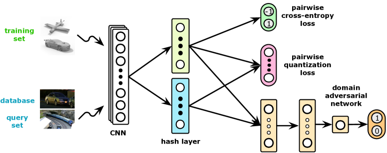
The architecture for learning the transfer hash function is shown in Figure 2, which is a hybrid deep architecture of a deep hashing network and a domain adversarial network. In the deep hashing network , we extend AlexNet (?), a deep convolutional neural network (CNN) comprised of five convolutional layers – and three fully connected layers –. We replace the layer with a new hash layer with hidden units, which transforms the network activation in -bit hash code by sign thresholding . Since it is hard to optimize sign function for its ill-posed gradient, we adopt the hyperbolic tangent (tanh) function to squash the activations to be within , which reduces the gap between the -layer representation and the binary hash codes , where . And a pairwise -distribution cross-entropy loss and a pairwise quantization loss are imposed on the hash codes. In domain adversarial network , we use the Multilayer Perceptrons (MLP) architecture adopted by (?). It accepts as inputs the hash codes generated by the deep hashing network and consists of three fully connected layers, with the numbers of units being . The last layer of output the probability of the input data belonging to a specific domain. And a cross-entropy loss is added on the output of the adversarial network. This hybrid deep network can achieve hash function learning through similarity relationship preservation and domain distribution alignment simultaneously, which enables image retrieval from the database in the target domain.
Hash Function Learning
To perform deep learning to hash from image data, we jointly preserve similarity relationship information underlying pairwise images and generate binary hash codes by Maximum A Posterior (MAP) estimation.
Given the set of pairwise similarity labels , the logarithm Maximum a Posteriori (MAP) estimation of training hash codes can be defined as
| (1) | ||||
where is likelihood function, and is prior distribution. For each pair of points and , is the conditional probability of their relationship given their hash codes and , which can be defined using the pairwise logistic function,
| (2) | ||||
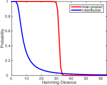
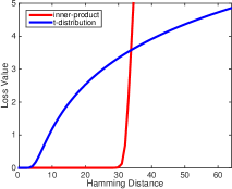
where is the similarity function of code pairs and and is the probability function. Previous methods (?; ?) usually adopt inner product function as similarity function and as probability function. However, from Figure 3, we can observe that the probability corresponds to these similarity function and probability function stays high when the Hamming distance between codes is larger than 2 and only starts to decrease when the Hamming distance becomes close to where is the number of hash bits. This means that previous methods cannot force the Hamming distance between codes of similar data points to be smaller than 2 since the probability cannot discriminate different Hamming distances smaller than sufficiently.
To tackle the above mis-specification of the inner product, we proposes a new similarity function inspiring by the success of -distribution with one degree of freedom for modeling long-tail dataset,
| (3) |
and the corresponding probability function is defined as . Similar to previous methods, these functions also satisfy that the smaller the Hamming distance is, the larger the similarity function value will be, and the larger will be, implying that pair and should be classified as “similar”; otherwise, the larger will be, implying that pair and should be classified as “dissimilar”. Furthermore, from Figure 3, we can observe that our probability w.r.t Hamming distance between code pairs decreases significantly when the Hamming distance is larger that , indicating that our loss function will penalize Hamming distance larger than for similar codes much more than previous methods. Thus, our similarity function and probability function perform better for search within Hamming Radius . Hence, Equation (2) is a reasonable extension of the logistic regression classifier which optimizes the performance of searching within Hamming Radius 2 of a query.
Similar to previous work (?; ?; ?), defining that where is the activation of hash layer, we relax binary codes to continuous codes since discrete optimization of Equation (1) with binary constraints is difficult and adopt a quantization loss function to control quantization error. Specifically, we adopt the prior for quantization of (?) as
| (4) |
where is the parameter of the exponential distribution.
By substituting Equations (2) and (4) into the MAP estimation in Equation (1), we achieve the optimization problem for similarity hash function learning as follows,
| (5) |
where is the trade-off parameter between pairwise cross-entropy loss and pairwise quantization loss , and is a set of network parameters. Specifically, loss is defined as
| (6) | ||||
Similarly the pairwise quantization loss can be derived as
| (7) |
where is the vector of ones. By the MAP estimation in Equation (5), we can simultaneously preserve the similarity relationship and control the quantization error of binarizing continuous activations to binary codes in source domain.
Domain Distribution Alignment
The goal of transfer hashing is to train the model on data of source domain and perform efficient retrieval from the database of target domain in response to the query of target domain. Since there is no relationship between the database points, we exploit the training data to learn the relationship among the database points. However, there is large distribution gap between the source domain and the target domain. Therefore, we should further reduce the distribution gap between the source domain and the target domain in the Hamming space.
Domain adversarial networks have been successfully applied to transfer learning (?) by extracting transferable features that can reduce the distribution shift between the source domain and the target domain. Therefore, in this paper, we reduce the distribution shifts between the source domain and the target domain by adversarial learning. The adversarial learning procedure is a two-player game, where the first player is the domain discriminator trained to distinguish the source domain from the target domain, and the second player is the base hashing network fine-tuned simultaneously to confuse the domain discriminator.
To extract domain-invariant hash codes , the parameters of deep hashing network are learned by maximizing the loss of domain discriminator , while the parameters of domain discriminator are learned by minimizing the loss of the domain discriminator. The objective of domain adversarial network is the functional:
| (8) |
where is the cross-entropy loss and is the domain label of data point . means belongs to target domain and means belongs to source domain. Thus, we define the overall loss by integrating Equations (5) and (8),
| (9) |
where is a trade-off parameter between the MAP loss and adversarial learning loss . The optimization of this loss is as follows. After training convergence, the parameters and will deliver a saddle point of the functional (9):
| (10) |
This mini-max problem can be trained end-to-end by back-propagation over all network branches in Figure 2, where the gradient of the adversarial loss is reversed and added to the gradient of the hashing loss . By optimizing the objective function in Equation (9), we can learn transfer hash codes which preserve the similarity relationship and align the domain distributions as well as control the quantization error of sign thresholding. Finally, we generate -bit hash codes by sign thresholding as , where is the sign function on vectors that for each dimension of , , if , otherwise . Since the quantization error in Equation (9) has been minimized, this final binarization step will incur small loss of retrieval quality for transfer hashing.
Experiments
We extensively evaluate the efficacy of the proposed TAH model against state of the art hashing methods on two benchmark datasets. The codes and configurations will be made available online.
Setup
NUS-WIDE111http://lms.comp.nus.edu.sg/research/NUS-WIDE.htm is a popular dataset for cross-modal retrieval, which contains 269,648 image-text pairs. The annotation for 81 semantic categories is provided for evaluation. We follow the settings in (?; ?; ?) and use the subset of 195,834 images that are associated with the 21 most frequent concepts, where each concept consists of at least 5,000 images. Each image is resized into pixels. We follow similar experimental protocols as DHN (?) and randomly sample 100 images per category as queries, with the remaining images used as the database; furthermore, we randomly sample 500 images per category (each image attached to one category in sampling) from the database as training points.
VisDA2017222https://github.com/VisionLearningGroup/taskcv-2017-public/tree/master/classification is a cross-domain image dataset of images rendered from CAD models as synthetic image domain and real object images cropped from the COCO dataset as real image domain. We perform two types of transfer retrieval tasks on the VisDA2017 dataset: (1) using real image query to retrieve real images where the training set consists of synthetic images (denoted by ); (2) using synthetic image query to retrieve synthetic images where the training set consists of real images (denoted by ). The relationship for training and the ground-truth for evaluation are defined as follows: if an image and a image share the same category, they are relevant, i.e. ; otherwise, they are irrelevant, i.e. . Similarly, we randomly sample 100 images per category of target domain as queries, and use the remaining images of target domain as the database and we randomly sample 500 images per category from both source domain and target domain as training points, where source domain data points have ground truth similarity information while the target domain data points do not.
We use retrieval metrics within Hamming radius 2 to test the efficacy of different methods. We evaluate the retrieval quality based on standard evaluation metrics: Mean Average Precision (MAP), Precision-Recall curves and Precision all within Hamming radius 2. We compare the retrieval quality of our TAH with ten classical or state-of-the-art hashing methods, including unsupervised methods LSH (?), SH (?), ITQ (?), supervised shallow methods KSH (?), SDH (?), supervised deep single domain methods CNNH (?), DNNH (?), DHN (?), HashNet (?) and supervised deep cross-domain method THN (?).
For fair comparison, all of the methods use identical training and test sets. For deep learning based methods, we directly use the image pixels as input. For the shallow learning based methods, we reduce the 4096-dimensional AlexNet features (?) of images. We adopt the AlexNet architecture (?) for all deep hashing methods, and implement TAH based on the Caffe framework (?). For the single domain task on NUS-WIDE, we test cross-domain method TAH and THN by removing the transfer part. For the cross-domain tasks on VisDA2017, we train single domain methods with data of source domain and directly apply the trained model to the query and database of another domain. We fine-tune convolutional layers – and fully-connected layers – copied from the AlexNet model pre-trained on ImageNet 2012 and train the hash layer and adversarial layers, all through back-propagation. As the layer and the adversarial layers are trained from scratch, we set its learning rate to be 10 times that of the lower layers. We use mini-batch stochastic gradient descent (SGD) with 0.9 momentum and the learning rate annealing strategy implemented in Caffe. The penalty of adversarial networks is increased from 0 to 1 gradually as RevGrad (?). We cross-validate the learning rate from to with a multiplicative step-size . We fix the mini-batch size of images as and the weight decay parameter as .
| Method | NUS-WIDE | VisDA2017 | ||||||||||
| 16 bits | 32 bits | 48 bits | 64 bits | 16 bits | 32 bits | 48 bits | 64 bits | 16 bits | 32 bits | 48 bits | 64 bits | |
| TAH | 0.722 | 0.729 | 0.692 | 0.680 | 0.465 | 0.423 | 0.433 | 0.404 | 0.672 | 0.695 | 0.784 | 0.761 |
| THN | 0.671 | 0.676 | 0.662 | 0.603 | 0.415 | 0.396 | 0.228 | 0.127 | 0.647 | 0.687 | 0.664 | 0.532 |
| HashNet | 0.709 | 0.693 | 0.681 | 0.615 | 0.412 | 0.403 | 0.345 | 0.274 | 0.572 | 0.676 | 0.662 | 0.642 |
| DHN | 0.669 | 0.672 | 0.661 | 0.598 | 0.331 | 0.354 | 0.309 | 0.281 | 0.545 | 0.612 | 0.608 | 0.604 |
| DNNH | 0.568 | 0.622 | 0.611 | 0.585 | 0.241 | 0.276 | 0.252 | 0.243 | 0.509 | 0.564 | 0.551 | 0.503 |
| CNNH | 0.542 | 0.601 | 0.587 | 0.535 | 0.221 | 0.254 | 0.238 | 0.230 | 0.487 | 0.568 | 0.530 | 0.445 |
| SDH | 0.555 | 0.571 | 0.517 | 0.499 | 0.196 | 0.238 | 0.229 | 0.212 | 0.330 | 0.388 | 0.339 | 0.277 |
| ITQ | 0.498 | 0.549 | 0.517 | 0.402 | 0.187 | 0.175 | 0.146 | 0.123 | 0.163 | 0.193 | 0.176 | 0.158 |
| SH | 0.496 | 0.543 | 0.437 | 0.371 | 0.154 | 0.141 | 0.130 | 0.105 | 0.154 | 0.182 | 0.145 | 0.123 |
| KSH | 0.531 | 0.554 | 0.421 | 0.335 | 0.176 | 0.183 | 0.124 | 0.085 | 0.143 | 0.178 | 0.146 | 0.092 |
| LSH | 0.432 | 0.453 | 0.323 | 0.255 | 0.122 | 0.092 | 0.083 | 0.071 | 0.130 | 0.145 | 0.122 | 0.063 |
Results
NUS-WIDE: The Mean Average Precision (MAP) within Hamming Radius 2 results are shown in Table 2. We can observe that on the classical task that database and query images are from the same domain, TAH generally outperforms state of the art methods defined on classical retrieval setting. Specifically, compared to the best method on this task, HashNet, and state of the art cross-domain method THN, we achieve absolute boosts of 0.031 and 0.053 in average MAP for different bits on NUS-WIDE, which is very promising.
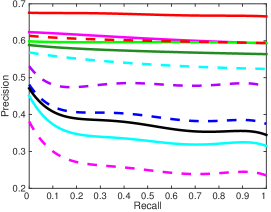
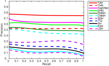
The precision-recall curves within Hamming Radius 2 based on 64-bits hash codes for the NUS-WIDE dataset are illustrated in Figure 4(a). We can observe that TAH achieves the highest precision at all recall levels. The precision nearly does not decrease with the increasing of recall, proving that TAH has stable performance for Hamming Radius 2 search.
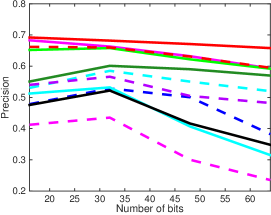
The Precision within Hamming radius 2 curves are shown in Figure 5(a). We can observe that TAH achieves the highest P@H=2 results on this task. When using longer codes, the Hamming space will become sparse and few data points fall within the Hamming ball with radius 2 (?). This is why most hashing methods perform worse on accuracy with very long codes. However, TAH achieves a relatively mild decrease on accuracy with the code length increasing. This validates that TAH can concentrate hash codes of similar data points to be within the Hamming ball of radius .
These results validate that TAH is robust under diverse retrieval scenarios. The superior results in MAP, precision-recall curves and Precision within Hamming radius 2 curves suggest that TAH achieves the state of the art performance for search within Hamming Radius 2 on conventional image retrieval problems where the training set and the database are from the same domain.
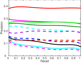
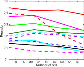
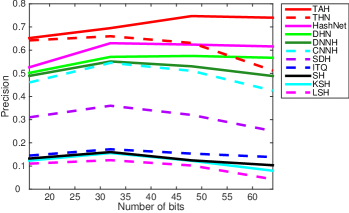
VisDA2017: The MAP results of all methods are compared in Table 2. We can observe that for novel transfer retrieval tasks between two domains of VisDA2017, TAH outperforms the comparison methods on the two transfer tasks by very large margins. In particular, compared to the best deep hashing method HashNet, TAH achieves absolute increases of 0.073 and 0.090 on the transfer retrieval tasks and respectively, validating the importance of mitigating domain gap in the transfer setting. Futhermore, compared to state of the art cross-domain deep hashing method THN, we achieve absolute increases of 0.140 and 0.096 in average MAP on the transfer retrieval tasks and respectively. This indicates that the our adversarial learning module is superior to MMD used in THN in aligning distributions. Similarly, the precision-recall curves within Hamming Radius 2 based on 64-bits hash codes for the two transfer retrieval tasks in Figure 4(b)-4(c) show that TAH achieves the highest precision at all recall levels. From the Precision within Hamming radius 2 curves shown in Figure 5(b)-5(c), we can observe that TAH outperforms other methods at different bits and has only a moderate decrease of precision when increasing the code length.
In particular, between two transfer retrieval tasks, TAH outperforms other methods with larger margin on task. Because the synthetic images contain less information and noise such as background and color than real images. Thus, directly applying the model trained on synthetic images to the real image task suffers from large domain gap or even fail. Transferring knowledge is very important in this task, which explains the large improvement from single domain methods to TAH. TAH also outperforms THN, indicating that adversarial network can match the distribution of two domains better than MMD, and the proposed similarity function based on -distribution can better concentrate data points to be within Hamming radius .
An counter-intuitive result is that the precision keeps unchanged while the recall increases, as shown in Figure 4. One plausible reason is that, we present a -distribution motivated hashing loss to enable Hamming space retrieval. Our new loss can concentrate as many data points as possible to be within Hamming ball with radius 2. This concentration property naturally leads to stable precision at different recall levels, i.e. the precision decreases much more slowly by increasing the recall.
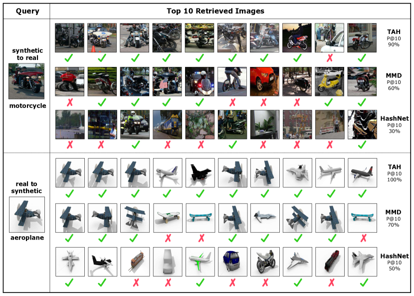
Furthermore, as an intuitive illustration, we visualize the top 10 relevant images for a query image for TAH, DHN and HashNet on and tasks in Figure 6. It shows that TAH can yield much more relevant and user-desired retrieval results.
The superior results of MAP, precision-recall curves and precision within Hamming Radius 2 suggest that TAH is a powerful approach to for learning transferable hash codes for image retrieval. TAH integrates similarity relationship learning and domain adversarial learning into an end-to-end hybrid deep architecture to build the relationship between database points. The results on the NUS-WIDE dataset already show that the similarity relationship learning module is effective to preserve similarity between hash codes and concentrate hash codes of similar points. The experiment on the VisDA2017 dataset further validates that the domain adversarial learning between the source and target domain contributes significantly to the retrieval performance of TAH on transfer retrieval tasks. Since the training and the database sets are collected from different domains and follow different data distributions, there is a substantial domain gap posing a major difficulty to bridge them. The domain adversarial learning module of TAH effectively close the domain gap by matching data distributions with adversarial network. This makes the proposed TAH a good fit for the transfer retrieval.
| Method | ||||||||
| 16 bits | 32 bits | 48 bits | 64 bits | 16 bits | 32 bits | 48 bits | 64 bits | |
| TAH-t | 0.443 | 0.405 | 0.390 | 0.364 | 0.660 | 0.671 | 0.717 | 0.624 |
| TAH-A | 0.305 | 0.395 | 0.382 | 0.331 | 0.605 | 0.683 | 0.725 | 0.724 |
| TAH | 0.465 | 0.423 | 0.433 | 0.404 | 0.672 | 0.695 | 0.784 | 0.761 |
Discussion
We investigate the variants of TAH on VisDA2017 dataset: (1) TAH-t is the variant which uses the pairwise cross-entropy loss introduced in DHN (?) instead of our pairwise -distribution cross-entropy loss; (2) TAH-A is the variant removing adversarial learning module and trained without using the unsupervised training data. We report the MAP within Hamming Radius 2 results of all TAH variants on VisDA2017 in Table 3, which reveal the following observations. (1) TAH outperforms TAH-t by very large margins of 0.031 / 0.060 in average MAP, which confirms that the pairwise cross-entropy loss learns codes within Hamming Radius 2 better than pairwise cross-entropy loss. (2) TAH outperforms TAH-A by 0.078 / 0.044 in average MAP for transfer retrieval tasks and . This convinces that TAH can further exploit the unsupervised train data of target domain to bridge the Hamming spaces of training dataset (real/synthetic) and database (synthetic/real) and transfer knowledge from training set to database effectively.
Conclusion
In this paper, we have formally defined a new transfer hashing problem for image retrieval, and proposed a novel transfer adversarial hashing approach based on a hybrid deep architecture. The key to this transfer retrieval problem is to align different domains in Hamming space and concentrate the hash codes to be within a small Hamming ball, which relies on relationship learning and distribution alignment. Empirical results on public image datasets show the proposed approach yields state of the art image retrieval performance.
Acknowledgments
This work was supported by the National Key Research and Development Program of China (2016YFB1000701), National Natural Science Foundation of China (61772299, 61325008, 61502265, 61672313) and TNList Fund.
References
- [Cao et al. 2016a] Cao, Y.; Long, M.; Wang, J.; Yang, Q.; and Yu, P. S. 2016a. Deep visual-semantic hashing for cross-modal retrieval. In KDD.
- [Cao et al. 2016b] Cao, Y.; Long, M.; Wang, J.; Zhu, H.; and Wen, Q. 2016b. Deep quantization network for efficient image retrieval. In AAAI. AAAI.
- [Cao et al. 2017a] Cao, Z.; Long, M.; Wang, J.; and Yang, Q. 2017a. Transitive hashing network for heterogeneous multimedia retrieval. In AAAI, 81–87.
- [Cao et al. 2017b] Cao, Z.; Long, M.; Wang, J.; and Yu, P. S. 2017b. Hashnet: Deep learning to hash by continuation. In ICCV.
- [Donahue et al. 2014] Donahue, J.; Jia, Y.; Vinyals, O.; Hoffman, J.; Zhang, N.; Tzeng, E.; and Darrell, T. 2014. Decaf: A deep convolutional activation feature for generic visual recognition. In ICML.
- [Erin Liong et al. 2015] Erin Liong, V.; Lu, J.; Wang, G.; Moulin, P.; and Zhou, J. 2015. Deep hashing for compact binary codes learning. In CVPR, 2475–2483. IEEE.
- [Fleet, Punjani, and Norouzi 2012] Fleet, D. J.; Punjani, A.; and Norouzi, M. 2012. Fast search in hamming space with multi-index hashing. In CVPR. IEEE.
- [Ganin and Lempitsky 2015] Ganin, Y., and Lempitsky, V. 2015. Unsupervised domain adaptation by backpropagation. In ICML.
- [Gionis et al. 1999] Gionis, A.; Indyk, P.; Motwani, R.; et al. 1999. Similarity search in high dimensions via hashing. In VLDB, volume 99, 518–529. ACM.
- [Gong and Lazebnik 2011] Gong, Y., and Lazebnik, S. 2011. Iterative quantization: A procrustean approach to learning binary codes. In CVPR, 817–824.
- [Gong et al. 2013] Gong, Y.; Kumar, S.; Rowley, H.; Lazebnik, S.; et al. 2013. Learning binary codes for high-dimensional data using bilinear projections. In CVPR, 484–491. IEEE.
- [He et al. 2016] He, K.; Zhang, X.; Ren, S.; and Sun, J. 2016. Deep residual learning for image recognition. CVPR.
- [Indyk and Motwani 1998] Indyk, P., and Motwani, R. 1998. Approximate nearest neighbors: Towards removing the curse of dimensionality. In STOC, 604–613. New York, NY, USA: ACM.
- [Jegou, Douze, and Schmid 2011] Jegou, H.; Douze, M.; and Schmid, C. 2011. Product quantization for nearest neighbor search. TPAMI 33(1):117–128.
- [Jia et al. 2014] Jia, Y.; Shelhamer, E.; Donahue, J.; Karayev, S.; Long, J.; Girshick, R.; Guadarrama, S.; and Darrell, T. 2014. Caffe: Convolutional architecture for fast feature embedding. In ACM MM. ACM.
- [Krizhevsky, Sutskever, and Hinton 2012] Krizhevsky, A.; Sutskever, I.; and Hinton, G. E. 2012. Imagenet classification with deep convolutional neural networks. In NIPS.
- [Kulis and Darrell 2009] Kulis, B., and Darrell, T. 2009. Learning to hash with binary reconstructive embeddings. In NIPS, 1042–1050.
- [Lai et al. 2015] Lai, H.; Pan, Y.; Liu, Y.; and Yan, S. 2015. Simultaneous feature learning and hash coding with deep neural networks. In CVPR.
- [Lew et al. 2006] Lew, M. S.; Sebe, N.; Djeraba, C.; and Jain, R. 2006. Content-based multimedia information retrieval: State of the art and challenges. TOMM 2(1):1–19.
- [Li, Wang, and Kang 2016] Li, W.-J.; Wang, S.; and Kang, W.-C. 2016. Feature learning based deep supervised hashing with pairwise labels. In IJCAI.
- [Liu et al. 2011] Liu, W.; Wang, J.; Kumar, S.; and Chang, S.-F. 2011. Hashing with graphs. In ICML. ACM.
- [Liu et al. 2012] Liu, W.; Wang, J.; Ji, R.; Jiang, Y.-G.; and Chang, S.-F. 2012. Supervised hashing with kernels. In CVPR. IEEE.
- [Liu et al. 2013] Liu, X.; He, J.; Lang, B.; and Chang, S.-F. 2013. Hash bit selection: a unified solution for selection problems in hashing. In CVPR, 1570–1577. IEEE.
- [Liu et al. 2014] Liu, X.; He, J.; Deng, C.; and Lang, B. 2014. Collaborative hashing. In CVPR, 2139–2146.
- [Liu et al. 2016] Liu, H.; Wang, R.; Shan, S.; and Chen, X. 2016. Deep supervised hashing for fast image retrieval. In CVPR, 2064–2072.
- [Norouzi and Blei 2011] Norouzi, M., and Blei, D. M. 2011. Minimal loss hashing for compact binary codes. In ICML, 353–360. ACM.
- [Norouzi, Blei, and Salakhutdinov 2012] Norouzi, M.; Blei, D. M.; and Salakhutdinov, R. R. 2012. Hamming distance metric learning. In NIPS, 1061–1069.
- [Norouzi, Punjani, and Fleet 2014] Norouzi, M.; Punjani, A.; and Fleet, D. J. 2014. Fast exact search in hamming space with multi-index hashing. TPAMI 36(6):1107–1119.
- [Salakhutdinov and Hinton 2007] Salakhutdinov, R., and Hinton, G. E. 2007. Learning a nonlinear embedding by preserving class neighbourhood structure. In AISTATS, 412–419.
- [Shen et al. 2015] Shen, F.; Shen, C.; Liu, W.; and Tao Shen, H. 2015. Supervised discrete hashing. In CVPR. IEEE.
- [Smeulders et al. 2000] Smeulders, A. W.; Worring, M.; Santini, S.; Gupta, A.; and Jain, R. 2000. Content-based image retrieval at the end of the early years. TPAMI 22(12):1349–1380.
- [Wang et al. 2014] Wang, J.; Shen, H. T.; Song, J.; and Ji, J. 2014. Hashing for similarity search: A survey. Arxiv.
- [Wang, Kumar, and Chang 2012] Wang, J.; Kumar, S.; and Chang, S.-F. 2012. Semi-supervised hashing for large-scale search. TPAMI 34(12):2393–2406.
- [Weiss, Torralba, and Fergus 2009] Weiss, Y.; Torralba, A.; and Fergus, R. 2009. Spectral hashing. In NIPS.
- [Xia et al. 2014] Xia, R.; Pan, Y.; Lai, H.; Liu, C.; and Yan, S. 2014. Supervised hashing for image retrieval via image representation learning. In AAAI, 2156–2162. AAAI.
- [Yang et al. 2017] Yang, E.; Deng, C.; Liu, W.; Liu, X.; Tao, D.; and Gao, X. 2017. Pairwise relationship guided deep hashing for cross-modal retrieval.
- [Yu et al. 2014] Yu, F. X.; Kumar, S.; Gong, Y.; and Chang, S.-F. 2014. Circulant binary embedding. In ICML, 353–360. ACM.
- [Zhang et al. 2014] Zhang, P.; Zhang, W.; Li, W.-J.; and Guo, M. 2014. Supervised hashing with latent factor models. In SIGIR, 173–182. ACM.
- [Zhu et al. 2016] Zhu, H.; Long, M.; Wang, J.; and Cao, Y. 2016. Deep hashing network for efficient similarity retrieval. In AAAI. AAAI.