Learning Sparse Graphs for Prediction of Multivariate Data Processes

Abstract

We address the problem of prediction of multivariate data process using an underlying graph model. We develop a method that learns a sparse partial correlation graph in a tuning-free and computationally efficient manner. Specifically, the graph structure is learned recursively without the need for cross-validation or parameter tuning by building upon a hyperparameter-free framework. Our approach does not require the graph to be undirected and also accommodates varying noise levels across different nodes. Experiments using real-world datasets show that the proposed method offers significant performance gains in prediction, in comparison with the graphs frequently associated with these datasets.

EDICS – SAS-STAT, DSP-GRAPH

I Introduction

Complex data-generating processes are often described using graph models [1, 2]. In such models, each node represents a component with a signal. Directed links between nodes represent their influence on each other. For example, in the case of sensor networks, a distance-based graph is often used to characterize the underlying process [3]. The estimation of undirected networks in the context of graph-Laplacian matrix has been considered extensively in the study of graph signals [4, 5, 6, 7, 8, 9]. Structural equation model and kernel-based methods have been employed for discovery of directed networks in the context of characterization and community analysis [10, 11]. The estimated graphs in these works are usually not applied explicitly for prediction over the graph but rather for characterization and in the context of recovering a graph that closely approximated an underlying graph.

In this paper, we are interested in graph models that are useful for prediction where the goal is to predict the signal values at a subset of nodes using information from the remaining nodes. To address this task, we aim to learn partial correlation graph models from a finite set of training data. Such graphs can be viewed as the minimal-assumption counterparts of conditional independence graphs [12, 13]. In the special case of Gaussian signals, the latter collapses into the former. Further, unlike many graph learning approaches which deal with undirected graphs using a graph-Laplacian approach, we do not assume our graph to be undirected.

As the size of a graph grows, the number of possible links between nodes grows quadratically. Thus to learn all possible links in a graph model requires large quantities of data. In many naturally occuring and human-made processes, however, the signal values at one node can be accurately predicted from a small number of other nodes. That is, there exists a corresponding sparse graph such that the links to each node are few, directly connecting only a small subset of the graph[14]. Sparse partial correlation based graphs have been considered earlier in the context of community identification and graph recovery [15, 16]. By taking sparsity into account it is possible to learn graph models with good predictive properties from far fewer samples. The methods for learning sparse models are usually posed as optimization problems and face two major challenges here. First, they require several hyperparameters to specify the appropriate sparsity-inducing constraints as shown below. Second, both tuning hyperparameters and solving the associated optimization problem is often computationally intractable and must be repeated each time the training dataset is augmented by a new data snapshot. This usually involves the use of some technique such as grid-search or some criterion such as Bayesian information (BIC) which adds to the computational complexity. We also note that these prior approaches also implicitly assume the noise or innovation variance to be equal across the different nodes of the graph.

Our contribution is a method for learning sparse partial correlation graph for prediction that achieves three goals:

• obviates the need to specify and tune large number of hyperparameters, which in the general case considered herein scales linearly with the number of nodes,

• computationally efficient with respect to the training data size: by exploiting its parallel structure the runtime scales linearly with the number of observations and quadratically with the number of nodes.

• accommodates varying noise levels across nodes.

The resulting prediction properties are demonstrated using real and synthetic datasets. Experiments with diverse real-world datasets show that our approach consistently produces graphs which result in superior prediction performance in comparison with some of the graph structures employed regularly in analysis of these datasets, e.g., geodesic graphs.

Reproducible research: Code for the method is available at https://github.com/dzachariah/sparse-pcg and https://www.researchgate.net/profile/Arun_Venkitaraman

II Problem formulation

We consider a weighted directed graph with nodes indexed by set $\mathcal{V}=\{1,2,\cdots,P\}$. Let $x_{i}$ denote a signal at the $i$th node and the link from node $j$ to $i$ has a weight $w_{ij}$. The signals from all nodes are collected in a $P$-dimensional vector $\mathbf{x}\sim p_{0}(\mathbf{x})$, where $p_{0}(\mathbf{x})$ is an unknown data generating process. We assume that its covariance matrix is full rank and, without loss of generality, consider the signals to be zero-mean. Next, we define the weights and related graph quantities.

II-A Partial correlation graph

A partial correlation graph is a property of $p_{0}(\mathbf{x})$ and can be derived as follows. Let

$$\begin{split}\widetilde{x}_{i}&=x_{i}-\operatorname{Cov}\big{[}x_{i},\mathbf{x}_{-(i,j)}\big{]}\operatorname{Cov}\big{[}\mathbf{x}_{-(i,j)}\big{]}^{-1}\mathbf{x}_{-(i,j)}\\ \widetilde{x}_{j}&=x_{j}-\operatorname{Cov}\big{[}x_{j},\mathbf{x}_{-(i,j)}\big{]}\operatorname{Cov}\big{[}\mathbf{x}_{-(i,j)}\big{]}^{-1}\mathbf{x}_{-(i,j)}\end{split}$$ (1)

denote the innovations at node $i$ and $j$ after partialling out the signals from all other nodes, contained in vector $\mathbf{x}_{-(i,j)}$. The weight of the link from node $j$ to node $i$ is then defined as

$$\boxed{w_{ij}\triangleq\frac{\operatorname{Cov}\big{[}\widetilde{x}_{i},\widetilde{x}_{j}\big{]}}{\operatorname{Var}\big{[}\widetilde{x}_{j}\big{]}},}$$ (2)

which quantifies the predictive effect of node $j$ on node $i$. The graph structure is thus encoded in a $P\times P$ weighted adjacency matrix $\mathbf{W}$, where the $ij$th element is equal to $w_{ij}$ and the diagonal elements are all zero. In many applications, we expect only a few links incoming to node $i$ to have nonzero weights.

We can write a compact signal representation associated with the graph by defining a latent variable $\varepsilon_{i}=x_{i}-\sum_{j\neq i}w_{ij}x_{j}$ at node $i$, with variance $\sigma^{2}_{i}$. By re-arranging, we can simply write

$$\mathbf{x}=\mathbf{W}\mathbf{x}+\boldsymbol{\varepsilon}$$ (3)

The variable $\varepsilon_{i}$ is zero mean and uncorrelated with the signal values on the right-hand side of row $i$ of (3), i.e., $\operatorname{E}[\mathbf{x}_{-i}\varepsilon_{i}]=\mathbf{0}$. This is shown by first using the fact that $\widetilde{x}_{j}$ is uncorrelated with all elements of $\mathbf{x}_{-(i,j)}$ [17] so that $\operatorname{E}[(x_{i}-\widetilde{x}_{i})\widetilde{x}_{j}]=0$. Therefore $\operatorname{E}[x_{j}\widetilde{x}_{j}]=\operatorname{Var}[\widetilde{x}_{j}]$ and $\operatorname{E}[\varepsilon_{i}\widetilde{x}_{j}]=\operatorname{E}[x_{i}\widetilde{x}_{j}]-w_{ij}\operatorname{Var}[\widetilde{x}_{j}]=\operatorname{E}[(x_{i}-\widetilde{x}_{i})\widetilde{x}_{j}]=0$ for all $j\neq i$. Consequently, $\operatorname{E}[\widetilde{\mathbf{x}}_{-i}\varepsilon_{i}]=\mathbf{0}$. Using the fact that $\mathbf{x}_{-i}$ is linearly related to its corresponding innovations $\widetilde{\mathbf{x}}_{-i}$, it follows that $\operatorname{E}[\mathbf{x}_{-i}\varepsilon_{i}]=\mathbf{0}$.

II-B Prediction

Having defined the weighted graph above, we now turn to the prediction problem. Given a signal $\mathbf{x}_{0}$ from a subset of nodes $\mathcal{V}_{0}\subset\mathcal{V}$, the problem is to predict unknown signal values at the remaining nodes $\mathcal{V}_{\star}$. An natural predictor of $\mathbf{x}_{\star}$ is:

$$\widehat{\mathbf{x}}_{\star}(\mathbf{W})=\mathbf{W}_{\star,0}\mathbf{x}_{0},$$ (4)

where $\mathbf{W}_{\star,0}$ denotes the corresponding submatrix of $\mathbf{W}$ of size $|\mathcal{V}_{\star}|\times|\mathcal{V}_{0}|$. We observe that (4) is a function of $\mathbf{W}$. Next, we develop a method for learning $\mathbf{W}$ from a dataset $\mathcal{D}=\big{\{}\mathbf{x}(1),\mathbf{x}(2),\dots,\mathbf{x}(N)\big{\}}$, where $\mathbf{x}(n)$ denotes the $n$th realization from $p_{0}(\mathbf{x})$. The learned graph $\widehat{\mathbf{W}}$ is then used to evaluate a predictor (4).

III Learning a sparse graph

Let $\mathbf{w}^{\top}_{i}$ be the $i$th row of $\mathbf{W}$ after removing the corresponding diagonal element. Then, for snapshot $n$, the $i$th row of (3) is given by

$$\begin{split}x_{i}(n)\>=\>\underbrace{\mathbf{w}^{\top}_{i}\mathbf{x}_{-i}(n)}_{\triangleq\widehat{x}_{i}(n;\mathbf{w}_{i})}\>+\>\varepsilon_{i}(n).\end{split}$$ (5)

A natural approach to learn a sparse graph $\mathbf{W}$ from $N$ training samples is:

$$\min_{\mathbf{W}:\;\|\mathbf{w}_{i}\|_{0}\leq K_{i},\;\forall i}\quad\sum_{i=1}^{P}\sum_{n=1}^{N}\left|x_{i}(n)-\widehat{x}_{i}(n;\mathbf{w}_{i})\right|^{2}$$ (6)

where the constraint $\|\mathbf{w}_{i}\|_{0}\leq K_{i}\ll P$ restricts the maximum number of directed links to each node. Let learned weights be denoted as $\mathbf{w}^{0}_{i}$, then $\widehat{x}_{i}(n;\mathbf{w}^{0}_{i})$ is a sparse predictor of $x_{i}(n)$ which we take as a reference. While this learning approach leads to strictly sparse weights, it has has two drawbacks. First, (6) is known to be NP-hard, and hence convex relaxations must be used practice [18]. Second, a user must specify suitable bounds $\{K_{i}\}$. Tractable convex relaxations of (6), such as the $\ell_{1}$-penalized Lasso approach [19, 20]

$$\min_{\mathbf{W}}\quad\sum_{i=1}^{P}\sum_{n=1}^{N}\left|x_{i}(n)-\widehat{x}_{i}(n;\mathbf{w}_{i})\right|^{2}+\lambda_{i}\|\mathbf{w}_{i}\|_{1},$$ (7)

avoid an explicit choice of $\{K_{i}\}$ but must in turn tune a set of hyperparameters $\{\lambda_{i}\}$ since the variances $\sigma^{2}_{i}$ are not uniform in general. With the appropriate choice of $\lambda_{i}$, the resulting deviation of $\widehat{x}_{i}(n;\widehat{\mathbf{w}}_{i})$ from $\widehat{x}_{i}(n;\mathbf{w}^{0}_{i})$ can be bounded [21]. Tuning these hyperparameters with e.g. cross-validation [22] is however computationally intractable, especially when $N$ becomes large. We note here that the approach taken by [15] and [16] in the context of graph discovery implicitly assumes that $\sigma^{2}_{i}$ is equal across nodes, which is a more restrictive assumption.

An alternative approach is to treat $\mathbf{w}_{i}$ as a random variable, with an expected value $\mathbf{0}$, prior to observing data from the $i$th node. Specifically, consider (5) conditioned on data from all other nodes $\mathbf{X}_{-i}=[\mathbf{x}^{\top}_{-i}(1)\,\cdots\,\mathbf{x}^{\top}_{-i}(N)]^{\top}$ and assume that

$$\operatorname{E}[\mathbf{w}_{i}|\mathbf{X}_{-i}]=\mathbf{0}\quad\text{and}\quad\operatorname{Cov}[\mathbf{w}_{i}|\mathbf{X}_{-i}]=\text{diag}(\boldsymbol{\pi}_{i}),$$

where $\boldsymbol{\pi}_{i}$ is a vector of variances. Under this conditional model, the MSE-optimal estimator of $\mathbf{w}_{i}$ after observing data from $i$th node $\underline{\mathbf{x}_{i}}=[x_{i}(1),\dots,x_{i}(N)]^{\top}$ is expressible as [17]:

$$\widehat{\mathbf{w}}_{i}(\boldsymbol{\pi},\sigma^{2})=\left(\mathbf{X}^{\top}_{-i}\mathbf{X}_{-i}+\sigma^{2}\text{diag}(\boldsymbol{\pi})^{-1}\right)^{-1}\mathbf{X}^{\top}_{-i}\underline{\mathbf{x}_{i}}.$$ (8)

Similar to the Empirical Bayes approach in [23], the hyperparameters $\boldsymbol{\pi}$ and $\sigma^{2}$ for each $i$ can be estimated by fitting the marginalized covariance model

$$\operatorname{Cov}[\underline{\mathbf{x}_{i}}|\mathbf{X}_{-i}]=\mathbf{X}_{-i}\text{diag}(\boldsymbol{\pi})\mathbf{X}^{\top}_{-i}+\sigma^{2}\mathbf{I}_{N}$$

to the sample covariance $\widehat{\operatorname{Cov}}[\underline{\mathbf{x}_{i}}|\mathbf{X}_{-i}]=\underline{\mathbf{x}_{i}}\underline{\mathbf{x}^{\top}_{i}}$ [24, 25]. It was shown in [26], that evaluating (8) at the estimated hyperparameters is equivalent to solving a convex, weighted square-root Lasso problem:

$$\widehat{\mathbf{w}}_{i}(\widehat{\boldsymbol{\pi}},\widehat{\sigma}^{2})=\operatorname*{arg\,min}_{\mathbf{w}_{i}}\;\|\underline{\mathbf{x}_{i}}-\mathbf{X}_{-i}\mathbf{w}_{i}\|_{2}+\sum_{j\neq i}\frac{\|\underline{\mathbf{x}_{j}}\|_{2}}{\sqrt{N}}|w_{ij}|,$$ (9)

This problem (aka. Spice) can be solved recursively with a runtime that scales as $\mathcal{O}(NP^{2})$ [27]. Since each $\widehat{\mathbf{w}}_{i}$ can be computed in parallel, this can be exploited to obtain $\widehat{\mathbf{W}}$ in the same runtime order. Moreover, under fairly general conditions, the deviation of $\widehat{x}_{i}(n;\widehat{\mathbf{w}}_{i})$ from $\widehat{x}_{i}(n;\mathbf{w}^{0}_{i})$ is bounded by known constants [28].

In sum, using the Spice approach (9) we learn a sparse graph $\widehat{\mathbf{W}}$ in a statistically motivated and computationally efficient manner without the need to search for or tune hyperparameters. Moreover, it accommodates varying noise levels across nodes.

IV Experiments

We apply the learning method to both synthesized and real-world multivariate data. We use a training set consisting of $N$ samples to learn a sparse graph. Then by evaluating (4) at $\widehat{\mathbf{W}}$, we perform prediction on separate testing sets. The performance is quantified using normalized mean-squared error evaluated over a test set. Specifically, we define the normalized prediction error as

$$\mbox{NPE}=\frac{\operatorname{E}\big{[}\|\mathbf{x}_{\star}-\widehat{\mathbf{x}}_{\star}\|^{2}_{2}\big{]}}{\operatorname{E}\big{[}\|\mathbf{x}_{\star}\|^{2}_{2}\big{]}}.$$

The expectation is calculated by averaging over different data samples. We evaluate the performance as a function of training set size $N$. The data is made zero-mean by subtracting the component-wise mean from the training and testing sets in all the examples considered. For the purposes of comparison, we also perform experiments with the least-squares (LS) estimate of $\mathbf{W}$ obtained as follows:

$$\min_{\mathbf{W}}\quad\sum_{i=1}^{P}\sum_{n=1}^{N}\left|x_{i}(n)-\widehat{x}_{i}(n;\mathbf{w}_{i})\right|^{2}$$ (10)

IV-A Synthesized graphs

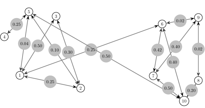
Figure 1: Graph structure with nonzero weights defined by $\mathbf{W}$.

We consider the graph shown in Figure 1 with the indicated edge weights $w_{ij}$ which is akin to a stochastic block model [29]. It consists of two densely connected communities of 5 nodes each with only two inter-community edges. To simulate network signals, we generate data as

$$\mathbf{x}(n)=(\mathbf{I}_{P}-\mathbf{W})^{-1}\boldsymbol{\varepsilon}(n),$$ (11)

where the elements of $\boldsymbol{\varepsilon}(n)$ are mutually uncorrelated and drawn uniformly from a Gaussian distribution with variances assigned as $\sigma^{2}_{i}\in(0,1]$. We generate a total of $2\times 10^{4}$ samples from which one half is used for training and remaining for testing by partitioning the total dataset randomly. All results are reported by averaging over 500 Monte Carlo simulations. For sake of illustration, we include an example of $\widehat{\mathbf{W}}$ from (9) when using $N=10^{4}$ training samples in Figure 2(a).

We perform prediction experiment using signals at $\mathcal{V}_{0}=\{2,4,6,8,10\}$ to predict the signals at $\mathcal{V}_{*}=\{1,3,5,7,9\}$. Figure 2(b) shows that NPE decreases with $N$ and ultimately converges to predictions using true $\mathbf{W}$.

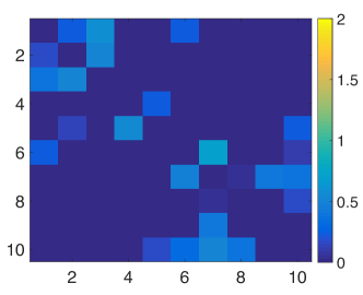
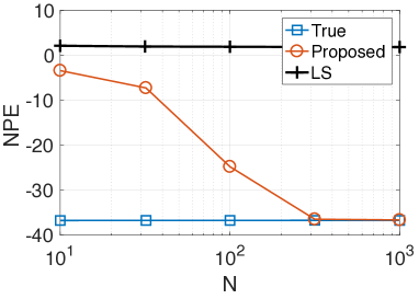
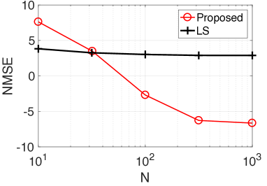
Figure 2: Results for synthesized graph. (a) Example of learned graph $\widehat{\mathbf{W}}$ using our approach. (b) Prediction errors in [dB], and (c) Normalized error of learned graph in [dB].

In Figure 2(d), we illustrate the rate of overall improvement of the learned graph as $N$ increases, measured as the normalized MSE $\operatorname{E}[\|\mathbf{W}-\widehat{\mathbf{W}}\|^{2}_{F}]$. We observe that the LS estimator performs poorly in terms of NPE. The NMSE of the LS estimator is also signficantly larger than of our approach. This is expected because the LS estimator is known to exhibit high variance.

IV-B Flow-cytometry data

We next consider flow-cytometry data used in [30], which consists of various instances of measurement of protein and phospholipid components in thousands of individual primary human immune system cells. The data consists of total 7200 responses of $P=11$ molecules to different perturbations which we divide the data into training and test sets. The partition is randomized and for each realization a graph $\widehat{\mathbf{W}}$ is learned. A learned graph is illustrated in Figure 3(a) using $N=3600$ samples. For the prediction task, we evaluate the performance using 100 Monte Carlo repetitions. For the sake of comparison, we also evaluate the performance with the sparse binary directed graph $\mathbf{W}^{\prime}$ proposed in [30]. This is because it has been used to encode the directed dependencies between nodes though not specifically designed for prediction. We make observations of the signal at nodes $\mathcal{V}_{0}=\{3,8,9\}$, noting that these proteins have the maximum number of connections in $\mathbf{W}^{\prime}$. Prediction is then performed for the signal values at the remaining nodes $\mathcal{V}_{\star}=\{1,2,4,5,6,7,10,11\}$. We observe from Figure 3(b) that the learned partial correlation graph $\widehat{\mathbf{W}}$ yields superior predictive performance on comparison with the reference graph $\mathbf{W}^{\prime}$. The improvements saturate beyond $N=10^{3}$ samples. As expected, the errors of the LS estimator are inflated by its higher variance.

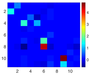
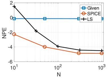
Figure 3: Results for flow-cytometry data: (a) Learned graph $\widehat{\mathbf{W}}$. (b) (a) Prediction error in [dB].

IV-C Temperature data for cities in Sweden

We next consider temperature data from the 45 most populated cities in Sweden. The data consists of 62 daily temperature readings for the period of November to December 2016 obtained from the Swedish Meteorological and Hydrological Institute [31]. In Figure 4, we show an instance of the learned graph $\widehat{\mathbf{W}}$ using $N=30$ observations. We observe that the graph is sparse as expected.

For the prediction task, we use a subset of $N$ observations for training and the remaining samples for testing, and perform 100 Monte Carlo repetitions. For reference, we compare the prediction performance with that of distance-based graph $\mathbf{W}^{\prime}$ with elements $w^{\prime}_{ij}=\exp\left(\frac{-d^{2}_{ij}}{\sum_{i,j}d_{ij}^{2}}\right)$ for all $i\neq j$ and $0$ for $i=j$. Here $d_{ij}$ denotes the geodesic distance between the $i$th and $j$th cities. This graph structure is commonly used in modelling relations between data points in spectral graph analysis and in the recently popular framework of graph signal processing [32], which makes it a relevant reference.

The cities are ordered in descending order of their population, and we use the temperatures of the bottom 40 cities to predict the top 5 cities. That is, $\mathcal{V}_{0}=\{1,2,3,4,5\}$ and $\mathcal{V}_{\star}=\{6,\cdots,45\}$. In Figure 4, we observe that the prediction performance using the learned graph $\widehat{\mathbf{W}}$ is high already at $N=10$ samples while using reference graph does not provide meaningful predictions. As with the earlier examples, we also plot the NPE values obtained for LS. We observe that the NPE for LS actually increases as the number of samples is increased. In our learnt graph in Figure4(a), the strongest edges are usually across cities which are geographically close. Further, a community structure is evident between nodes 1 to 15 and between nodes 20 to 40. This agrees with the observation that the most populated cities (nodes 1 to 15) mostly all lie in the south of Sweden and hence, are similar in geography and population. Such an observation can also be made about the nodes from 20 to 40, since they correspond to the relatively colder northern cities.

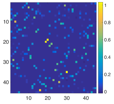
Figure 4: Results for temperature data: (a) Learned graph $\widehat{\mathbf{W}}$. (b) Prediction error in [dB].

IV-D 64-channel EEG data

Finally, we consider 64-channel electroencephalogram (EEG) signals obtained by placing 64 electrodes at various positions on the head of a subject and recorded different time-instants [33]. We divide the data consisting of 7000 samples into training and test sets using 100 Monte Carlo repetitions. An example of a learned graph using our approach is shown in Figure 5(a). For reference, we compare the prediction performance with that obtained using a diffusion-based graph $\mathbf{W}^{\prime}$, where $w^{\prime}_{ij}=\exp\left(-\frac{\|\mathbf{r}_{i}-\mathbf{r}_{j}\|_{2}^{2}}{\sum_{i,j}\|\mathbf{r}_{i}-\mathbf{r}_{j}\|_{2}^{2}}\right),$ and $\mathbf{r}_{j}$ is the vector of 500 successive signal samples from a separate set of EEG signals at the $j$th electrode or node. In Figure 5(b) we observe that predictive performance using the learned partial correlation graph is substantially better than using the diffusion-based reference graph and reaches a value close to $-10$dB even at very low training sample sizes. We observe that the NPE with LS estimator remains large even when $N$ is increased.

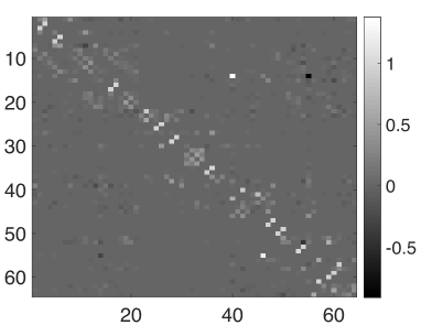
Figure 5: Results for EEG data: (a) Learned graph $\widehat{\mathbf{W}}$. (b) Prediction error in [dB].

V Conclusion

We have addressed the problem of prediction of multivariate data process by defining underlying graph model. Specifically, we formulated a sparse partial correlation graph model and associated target quanties for prediction. The graph structure is learned recursively without the need for cross-validate or parameter tuning by building upon a hyperparameter-free framework. Using real-world data we showed that the learned partial correlation graphs offer superior prediction performance compared with standard weighted graphs associated with the datasets.

References

- [1] E. D. Kolaczyk, Statistical Analysis of Network Data: Methods and Models. Springer Berlin, 2009.
- [2] A.-L. Barabási and M. Pósfai, Network Science. Cambridge Univ. Press, 2016.
- [3] D. I. Shuman, S. Narang, P. Frossard, A. Ortega, and P. Vandergheynst, “The emerging field of signal processing on graphs: Extending high-dimensional data analysis to networks and other irregular domains,” IEEE Signal Process. Mag., vol. 30, no. 3, pp. 83–98, 2013.
- [4] D. Xiaowen, T. Dorina, F. Pascal, and V. Pierre, “Learning laplacian matrix in smooth graph signal representations,” IEEE Trans. Sig. Proc., vol. 64, pp. 6160–6173, Dec. 2016.
- [5] D. Thanou, X. Dong, D. Kressner, and P. Frossard, “Learning heat diffusion graphs,” IEEE Trans. Signal Info. Process. Networks, vol. 3, pp. 484–499, Sept 2017.
- [6] S. Segarra, A. G. Marques, G. Mateos, and A. Ribeiro, “Network topology inference from spectral templates,” IEEE Trans. Signal Info. Process. Networks, vol. 3, pp. 467–483, Sept 2017.
- [7] R. Shafipour, S. Segarra, A. G. Marques, and G. Mateos, “Network topology inference from non-stationary graph signals,” Proc. IEEE Int. Conf. Acoust., Speech Signal Process., pp. 5870–5874, March 2017.
- [8] B. Pasdeloup, V. Gripon, G. Mercier, D. Pastor, and M. G. Rabbat, “Characterization and inference of graph diffusion processes from observations of stationary signals,” IEEE Trans. Signal Info. Process. Networks, pp. 1–1, 2017.
- [9] S. P. Chepuri, S. Liu, G. Leus, and A. Hero, “Learning sparse graphs under smoothness prior,” Proc. IEEE Int. Conf. Acoust., Speech Signal Process., pp. 6508–6512, 2017.
- [10] X. Cai, J. A. Bazerque, and G. B. Giannakis, “Inference of gene regulatory networks with sparse structural equation models exploiting genetic perturbations,” PLOS Comput. Biology, vol. 9, pp. 1–13, 05 2013.
- [11] Y. Shen, B. Baingana, and G. B. Giannakis, “Kernel-based structural equation models for topology identification of directed networks,” IEEE Trans. Signal Process., vol. 65, pp. 2503–2516, May 2017.
- [12] D. Koller and N. Friedman, Probabilistic Graphical Models. MIT Press, 2009.
- [13] A. A. Amini, B. Aragam, and Q. Zhou, “Partial correlation graphs and the neighborhood lattice,” ArXiv e-prints, Nov. 2017.
- [14] D. Angelosante and G. B. Giannakis, “Sparse graphical modeling of piecewise-stationary time series,” Proc. IEEE Int. Conf. Acoust., Speech Signal Process., pp. 1960–1963., May 2011.
- [15] N. Meinshausen and P. Bühlmann, “High-dimensional graphs and variable selection with the lasso,” Annal. Stat., vol. 34, no. 3, pp. 1436–1462, 2006.
- [16] J. Peng, P. Wang, N. Zhou, and J. Zhu, “Partial correlation estimation by joint sparse regression models,” J. Amer. Stat. Assoc., vol. 104, no. 486, pp. 735–746, 2009.
- [17] T. Kailath, A. H. Sayed, and B. Hassibi, Linear estimation. Prentice-Hall, Inc., 2000.
- [18] D. L. Donoho, M. Elad, and V. N. Temlyakov, “Stable recovery of sparse overcomplete representations in the presence of noise,” IEEE Trans. Inf. Theor., vol. 52, pp. 6–18, Jan. 2006.
- [19] R. Tibshirani, “Regression shrinkage and selection via the lasso,” Journal of the Royal Statistical Society, Series B, vol. 58, pp. 267–288, 1994.
- [20] S. Yang and E. D. Kolaczyk, “Target detection via network filtering,” IEEE Transactions on Information Theory, vol. 56, pp. 2502–2515, May 2010.
- [21] P. Bühlmann and S. Van De Geer, Statistics for high-dimensional data: methods, theory and applications. Springer Science & Business Media, 2011.
- [22] T. Hastie, R. Tibshirani, and J. Friedman, The Elements of Statistical Learning: Data Mining, Inference, and Prediction, Second Edition. Springer Series in Statistics, Springer New York, 2009.
- [23] J. Berger, Statistical Decision Theory and Bayesian Analysis. Springer Series in Statistics, Springer, 1985.
- [24] T. W. Anderson, “Linear latent variable models and covariance structures,” Journal of Econometrics, vol. 41, no. 1, pp. 91–119, 1989.
- [25] P. Stoica, P. Babu, and J. Li, “New method of sparse parameter estimation in separable models and its use for spectral analysis of irregularly sampled data,” IEEE Trans. Signal Processing, vol. 59, no. 1, pp. 35–47, 2011.
- [26] P. Stoica, D. Zachariah, and J. Li, “Weighted SPICE: A unifying approach for hyperparameter-free sparse estimation,” Digital Signal Processing, vol. 33, pp. 1–12, 2014.
- [27] D. Zachariah and P. Stoica, “Online hyperparameter-free sparse estimation method,” IEEE Trans. Signal Processing, vol. 63, pp. 3348–3359, July 2015.
- [28] D. Zachariah, P. Stoica, and T. B. Schön, “Online learning for distribution-free prediction,” arXiv preprint arXiv:1703.05060, 2017.
- [29] M. E. J. Newman, Networks: An Introduction. Oxford University Press, 2010.
- [30] K. Sachs, O. Perez, D. Pe’er, D. A. Lauffenburger, and G. P. Nolan, “Causal protein-signaling networks derived from multiparameter single-cell data,” Science, vol. 308, no. 5721, pp. 523–529, 2005.
- [31] “Swedish Meteorological and Hydrological Institute (SMHI).”
- [32] A. Sandryhaila and J. M. F. Moura, “Discrete signal processing on graphs,” IEEE Trans. Signal Process., vol. 61, no. 7, pp. 1644–1656, 2013.
- [33] A. L. Goldberger, L. A. N. Amaral, L. Glass, J. M. Hausdorff, P. C. Ivanov, R. G. Mark, J. E. Mietus, G. B. Moody, C.-K. Peng, and H. E. Stanley, “Physiobank, physiotoolkit, and physionet,” vol. 101, no. 23, pp. e215–e220, 2000.