HU-EP-17/28, arXiv:1712.04527
The Matrix Element Method at next-to-leading order QCD for hadronic collisions: Single top-quark production at the LHC as an example application
Abstract
Recently, a general algorithm to extend the Matrix Element Method (MEM) by taking into account next-to-leading-order (NLO) corrections in quantum chromodynamics (QCD) has been presented. In this article, the algorithm is applied to the most general case that coloured partons are encountered in the initial as well as the final state. This represents a substantial extension compared to previous work. As a concrete example, the production of single top quarks at the LHC is studied. We present in detail the generation of unweighted events following the NLO predictions. By treating these events as the result of a toy experiment, we show the first proof-of-principle application of the Matrix Element Method at NLO QCD for hadronic jet production. As an illustration, we study the determination of the top-quark mass. We find that—apart from elevating the powerful MEM to a sound theoretical foundation at NLO—the inclusion of the NLO corrections can lead to sizeable effects compared to the Matrix Element Method relying on leading-order predictions only. Furthermore, we find that the incorporation of the NLO corrections is mandatory to obtain reliable estimates of the theoretical uncertainties. In addition, this work shows that measuring the top-quark mass using the MEM in single top-quark production offers an interesting alternative to mass measurements in top-quark pair production.
1 Introduction
In recent years multivariate methods have been proven to be instrumental for the data analysis at the Large Hadron Collider (LHC). Neuronal networks (NN), boosted decision trees (BDT) and the Matrix Element Method (MEM) as specific examples belong to the standard techniques employed in the LHC analysis today. Among these methods the Matrix Element Method is of particular interest since the approach provides a very clean statistical interpretation based on a direct link between theory and event reconstruction. It can be used for signal-background discrimination as well as for parameter extraction. The Matrix Element Method as introduced in ref. [1, 2] relies on the assumption that the differential cross section can be interpreted as the probability distribution to observe a particular event signature. Under this assumption, the cross section is used to define a likelihood function. Parameter determinations can be performed by maximising this likelihood with respect to the model parameters used in the theoretical predictions. Signal-background discrimination can be performed by defining likelihood ratios for signal+background and the background only hypotheses. Both aspects have been pioneered in the top-quark analysis at the Tevatron. In the early days of the top-quark discovery the Matrix Element Method was used to determine the top-quark mass based on events only [3, 4, 5]. See ref. [6] for an introduction to the Matrix Element Method in the context of top-quark mass measurements. In the single top-quark studies the method was instrumental to separate the signal from the overwhelming background (see e.g. ref. [7]). More recent applications can be found in refs. [8, 9, 10, 11, 12, 13, 14, 15, 16]. An automation of the Matrix Element Method at leading order is presented in ref. [17].
The strength of the Matrix Element Method, namely offering a clean statistical interpretation, also points to a potential weakness: The method will fail to produce reliable results if the theoretically calculated cross section does not provide a decent description of the underlying probability distribution. In this case the statistical analysis shows that in general parameter extraction with the Matrix Element Method no longer provides an unbiased estimator. In principle, this does not preclude the usage of the Matrix Element Method for parameter extraction, since the bias can be removed by an additional calibration procedure. However, it would make the application of the Matrix Element Method less attractive because the calibration introduces additional uncertainties and might rely on auxiliary modelling. Facing the increasing precision current experiments are aiming for, it is thus mandatory to include higher-order QCD corrections to the cross section predictions used in the Matrix Element Method. However, so far the Matrix Element Method as applied in the experimental analysis relies on leading-order cross section predictions only. In recent years various attempts have been made to extend the Matrix Element Method to NLO. In ref. [18] the effect of QCD radiation is studied as a first step in this direction. In refs. [19, 20] the information from the hard LO matrix element is combined with a parton shower. In ref. [21] a method is presented to consider NLO QCD corrections within the Matrix Element Method for the production of uncoloured final states. A first application is studied in ref. [22]. In ref. [23] the inclusion of hadronic production of jets by mapping NLO and LO jets with a longitudinal boost along the beam axis to remove the unbalanced transverse momentum is investigated. However, no general algorithm to include NLO QCD corrections for the hadronic production of coloured partons within the Matrix Element Method is presented. Only very recently a complete algorithm to systematically include NLO QCD corrections within the Matrix Element Method has been presented in ref. [24]. As a proof of concept the Drell-Yan process and top-quark pair production in - annihilation has been studied in ref. [24]. While ref. [24] relies on a well-motivated modification of the clustering prescription used within the jet algorithm, it was shown in ref. [25] how the method can be extended avoiding the modification of the clustering prescription. However, the extension presented in ref. [25] relies on the numerical solution of a system of non-linear equations and the proof of the feasibility of this approach in practical applications is still missing.
The examples studied in ref. [24] were chosen to offer sufficient complexity to test all the aspects of the proposed algorithm while still being simple enough to not pose any challenge to the numerical implementation. However, phenomenologically wise the two examples are of limited interest although the studies of top-quark pair production in -annihilation may provide useful information for a future linear collider. In this article we apply the Matrix Element Method at NLO QCD to hadronic single top-quark production as a particular example for the general case that coloured partons occur in the initial as well as the final state. Because of the large backgrounds single top-quark production is very challenging and the usage of the Matrix Element Method is well motivated. Although top-quark production in hadronic collisions is dominated by top-quark pair production, single top-quark production plays a central role in top-quark physics at the LHC, since it provides complementary information. In particular, single top-quark production is a unique source of polarised top-quarks and allows detailed tests of the structure of the coupling to the -boson and gives access to the Cabbibo-Kobayashi-Maskawa matrix element .
In leading order three different production modes are distinguished in the Standard Model (SM):
| (1.1) | |||||
| (1.2) | |||||
| (1.3) |
At the LHC single top-quark production is dominated by the -channel followed by the -channel. The -channel total cross section has been precisely measured at the LHC at 7, 8 and 13 TeV by both CMS and ATLAS [26, 27, 28, 29, 30, 31, 32, 33, 34].
The -channel production gives only a very small contribution at the LHC. Because of the complicated backgrounds the signal is difficult to extract and only recently evidence has been reported by the ATLAS collaboration [11]. In ref. [11] the usage of the Matrix Element Method has been proven instrumental to extract the signal. The independent measurement of - and -channel production provides useful information to constrain physics beyond the Standard Model (see for example ref. [7] for an overview of recent results). Anticipating further experimental progress, we present in this article the application of the Matrix Element Method to - and -channel production including NLO QCD corrections, relying on existing results for the NLO corrections. Next-to-leading order results for the - and -channel have been known for quite a while (see e.g. ref. [35, 36] and are available in numerical implementations like MCFM (see ref. [37]) or HATHOR (see ref. [38]).
In this article we apply the algorithm presented in ref. [24] to single top-quark production at the LHC. We present the first application of the MEM at NLO to the hadronic production of jets originating from coloured final state partons. As a proof of concept, we generate unweighted - and -channel single top-quark events following the NLO predictions (with and without a veto on an additional resolved jet) and apply the MEM at NLO to reproduce the top-quark input mass from these events.
The article is organised as follows. In section 2 we give a brief review of the Matrix Element Method. In particular, we focus on aspects relevant for incorporating NLO QCD corrections. Furthermore, we give a short description of the approach presented in ref. [24] to extent the Matrix Element Method to NLO accuracy. In section 3 we discuss the generation of unweighted events following the NLO cross section predictions. By comparing with a traditional parton level Monte Carlo we also validate the entire procedure. We study an inclusive as well as an exclusive event definition. The exclusive event definition in which we veto additional jet emission is used to allow a more detailed test of the procedure. Interpreting the unweighted events generated in section 3 as the result of a pseudo-experiment, we illustrate the application of the Matrix Element Method including NLO QCD corrections in section 4. As a detailed test of the method, we simulate a measurement of the top-quark mass. The main results are summarised in section 5.
2 The Matrix Element Method
2.1 The Matrix Element Method in the Born approximation
To set up the notation used in this article, we briefly review the essence of the Matrix Element Method in the Born approximation. A detailed description focusing on top-quark mass measurements with the Matrix Element Method is given for example in ref. [6]. The basic idea is to treat the normalised differential cross section calculated from the squared matrix elements as the probability distribution to observe a specific event in the final state. We may think of a parton event as a collection of partonic momenta. However, for the following discussion it turns out to be useful to generalise the event definition to an arbitrary collection of variables used to describe the event. This set of variables which we may collect into a vector does not need to be complete in the sense that all available information about the event can be reconstructed. The dimension of the vector may thus be smaller than the number of independent variables , where denotes the number of outgoing partons. In the spirit of the Matrix Element Method the probability distribution for the production of an event described by is then described by the (parameter-dependent) differential cross section
| (2.1) |
The vector collects all the parameters e.g. couplings and masses on which the cross section depends. The normalisation factor is given by the (parameter-dependent) fiducial cross section:
| (2.2) |
The probability distribution is thus normalised to one. The differential cross section is defined schematically through
| (2.3) | |||||
As usual, the denote the parton distribution functions and the hadronic centre-of-mass energy squared. The sum runs over all possible parton configurations in the initial state. If more than one sub-process contributes to a given event signature (e.g. background) the right hand side of eq. (2.3) needs to be extended to include a sum over all contributing sub-processes. The partonic variables used to parameterise the -parton phase space measure as well as the squared matrix elements are collected in . The function maps the integration variables to the variables used to describe the partonic event. In experiments we do not observe partons but hadrons and leptons. Using again a collection of variables to describe the hadronic event as observed in the experiment the probability distribution reads:
| (2.4) |
where the ‘transfer function’ describes the probability to observe a partonic event as an hadronic event . The transfer functions have to be normalised
| (2.5) |
in order to ensure the correct normalisation of the probability density. In most applications one assumes that factorises into a product of transfer functions describing the transition of individual partons and leptons. For leptons where the energy and the direction of flight can be measured with good accuracy the transfer functions are often modelled using narrow Gaussian distributions. For unobserved particles the transfer function is replaced by leading to an integration of the related variables over the full phase space and the aforementioned reduction of variables used to describe the differential cross section. For simplicity, we assume in the following an ideal detector where the transfer functions are replaced by -functions. Note that the transfer functions model a variety of different effects. They form an interface between theoretical predictions and experimental observations and thus bridge the gap between the two. Their impact may be reduced by improving the theoretical modelling (e.g. considering instead of final states) or including higher-order corrections in the predictions. Furthermore, it is conceivable that the experimental data could be unfolded to some intermediate level further reducing the impact of the transfer functions. Using -functions may thus provide a useful first approximation. As far as the conceptual aspects of the method used in this article are concerned, the inclusion of non-trivial transfer functions will not change any of the arguments presented here. Non-trivial transfer function would only add additional integrations. In practice however, the inclusion of more realistic transfer functions may lead to additional technical problems as far as the numerical integration is concerned. This is well known from the application of the Matrix Element Method in leading-order. We thus consider the results presented in this article only as a first step towards a more realistic analysis. Additional technical improvements may be required to include transfer functions as determined in the experimental analysis.
We now briefly review the possibilities to use the Matrix Element Method for signal-background discrimination and parameter estimation. In addition, we introduce the concept of the extended likelihood and collect some useful properties of estimators extracted with the Matrix Element Method.
Signal-background discrimination
As mentioned before, eq. (2.3) may include signal as well as background processes. In ref. [39] it has been argued that calculating the probability distribution independently for signal and signal plus background an optimal discriminator can be constructed using the ratio. Thus, the Matrix Element Method makes optimal use of the information contained in an event sample. Recent experimental work on establishing -channel single top-quark production provides a nice example [11] of the usefulness of the Matrix Element Method in establishing “signals”.
Parameter extraction
However, this is not the only application of the Matrix Element Method. Since in eq. (2.4) depends on the theory parameters the Matrix Element Method can also be used to determine the model parameters. For a given event sample the likelihood
| (2.6) |
is a function of the model parameters. Maximising the likelihood with respect to the model parameters yields an estimator for the true parameters. This technique has been applied with great success to the top-quark mass determination at the Tevatron collider (see refs. [3, 4, 5]).
Extended likelihood
The likelihood as defined in eq. (2.6) only depends on the normalised differential cross sections and therefore only on the relative distribution of the events in the event sample . The total cross section and therefore the expected number of observed events may also depend on the model parameters. To make use of the additional information contained in the size of the event sample the so-called extended likelihood function can be applied (see e.g. ref. [40]). Here the number of observed events is assumed to be a random number distributed according to a Poisson distribution with expectation value , where denotes the integrated luminosity of the collider. The extended likelihood function is given by the likelihood in eq. (2.6) multiplied with the Poisson probability to observe an event sample of size under the parameter-dependent model assumption (here incorporated in ):
| (2.7) | |||||
In the extended likelihood the normalisation in front of the differential cross section cancels. The Matrix Element Method employing extended likelihoods is thus not only sensitive to the relative distribution but also to the total number of observed events. Using the additional information contained in the absolute number of observed events may result in a more efficient estimator when the Matrix Element Method is used within the context of parameter determination. However, the integrated luminosity is needed in eq. (2.7) which may introduces an additional uncertainty potentially spoiling the gain in efficiency. We shall come back to this issue when we discuss as an illustration the top-quark mass extraction in detail in section 4.2.
Properties of Matrix Element Method estimators
Since the likelihood as defined in eq. (2.6) depends on the measured event sample which follows a probability distribution and can thus be seen as a collection of random numbers, the Maximum Likelihood estimator is itself a random number with expectation value and variance . The variance of an estimator is bounded from below by the Rao-Cramér-Fréchet inequality (see ref. [41]). In the large sample limit Maximum Likelihood estimators approach the Rao-Cramér-Fréchet bound making them in a sense maximally efficient. Furthermore, in this limit Maximum Likelihood estimators exhibit ‘asymptotic normality’, meaning that they are distributed according to a Gaussian normal distribution with and (see ref. [41]). A potential disadvantage of parameter extraction based on Maximum Likelihood is that the estimator is prone to have a non-vanishing bias
| (2.8) |
if the analysed data is not distributed exactly according to the assumed probability density. In practice, such biases can be accounted for by the experiments through a calibration of the method, however, at the cost of introducing associated uncertainties. Therefore it is preferable to reduce the bias by modelling the true probability density as accurately as possible. This is an important motivation to extend the Matrix Element Method to NLO accuracy.
2.2 The Matrix Element Method at next-to-leading order accuracy in QCD
It is well known that for many processes the Born approximation gives only a rough estimate and higher-order corrections are sizeable. Furthermore, high energetic hadron scattering leads to an increase in jet activity which needs to be modelled appropriately unless the additional jet activity is vetoed which would however lead to a reduction of the event sample and may also spoil the convergence of the perturbative expansion. Higher-order corrections lead also to a better modelling of the jets and are mandatory to obtain more realistic predictions. In Born approximation each parton is identified with a jet. Only beyond leading order the recombination of two partons to form a jet occurs. It is thus highly desirable to include higher-order corrections in the Matrix Element Method. When the Matrix Element Method is used for parameter determinations higher-order corrections are crucial: in general, next-to-leading order corrections are required to unambiguously define the renormalisation scheme. As long as only leading-order calculations are used, the renormalisation scheme is not defined.
Extending the Matrix Element Method to include higher-order corrections is however non-trivial. To understand the origin of the difficulties we start with the general structure of NLO corrections. Schematically, the differential cross section including NLO corrections reads:
| (2.9) | |||||
We denote with () the Born and virtual (real) contributions to the next-to-leading order differential cross section. () defines the jet function which implicitly introduces a mapping of the parton momenta to the jet momenta and implements phase space cuts depending on the jet momenta. defines the jet function for the -parton phase space in which all partons are resolved as individual jets and no recombination occurs. It is in fact through that a jet is modelled for the first time in a non-trivial way within perturbation theory. Together with the contribution due to this leads to the aforementioned improved description of additional jet activity.
As stated above, no recombination can occur in leading order and the jet momenta are identified with the parton momenta:
| (2.10) |
The jet functions for identifying the partons with jets have the form
| (2.11) |
with functions which encode whether the jet momenta are resolved as a -jet final state. (The same is also true for the contribution involving .) Since in leading order the mapping is trivial it has been omitted in eq. (2.3) although the jet function might be required to render the cross section finite in cases in which the leading-order predictions contain already soft and/or collinear singularities (e.g. ). The virtual corrections can thus be treated in a similar way as the Born approximation, ignoring for the moment that they may contain soft and collinear singularities which must be cancelled. In case of the real corrections, the situation is more involved since now recombination can occur and the jet momenta are in general non-trivial functions of the partonic momenta with the mapping depending on the phase space region
| (2.12) |
The jet functions for the recombinations of partons to form jets have the form
| (2.13) |
where the mapping from the parton momenta to the jet momenta is given by the functional dependences of the jet momenta on the parton momenta in eq. (2.12). Note that the differential cross section is differential in ‘jet variables’ and not in partonic variables: We use the function to relate the variables used to describe the differential cross section to the jet momenta. Strictly speaking this detour is not required and one could avoid introducing jets as long as the definition of variables used to describe the final state is infrared safe. Using jet momenta in intermediate steps however, simplifies the construction of infrared safe distributions and leads to a general algorithm to extend the Matrix Element Method to NLO accuracy. Inspecting eq. (2.9) in more detail various problems, preventing a straightforward application, become obvious:
-
1.
The first two contributions are individually ill-defined because of soft and collinear singularities. Only in the sum of the two a finite result is obtained.
-
2.
Being differential in the measured jet observables introduces conditions on the recombination of unresolved real parton momenta to form respective jet momenta corresponding to the fixed values in . These conditions prevent an efficient numerical integration of the real contribution.
-
3.
In the -parton contribution the jets are identified with the partons. As a consequence the jet momenta satisfy the -parton kinematics, i.e. the jet momenta respect the on-shell condition as well as four-momentum conservation. For the recombined jets obtained from -parton momenta this is in general not the case. In particular, defining the momentum of the recombined jet as the sum of the combined parton momenta violates the on-shell condition unless the recombined momenta are strictly collinear. As a consequence the jet momenta cannot be used to evaluate which would be the naive way to establish a point wise cancellation of the soft and collinear divergences.111Note that this is not a problem in conventional parton-level Monte-Carlos which always integrate over finite phase space regions and the cancellation works at the level of the integral.
In ref. [24] it has been argued, that the last two obstacles can be overcome using modified jet algorithms relying on a clustering instead of a recombination usually applied. The additional spectator particle allows to guarantee four-momentum conservation and the on-shell conditions at the same time. In practice, a recombination inspired by the phase space parameterisation used in the Catani-Seymour dipole subtraction method [42, 43] is used in ref. [24]. This technique allows a factorisation of the -parton phase space measure into an unresolved and a resolved contribution. Schematically, this factorisation reads:
| (2.14) |
where denotes the phase space of the jets obtained after recombination, and parameterises the unresolved phase space leading to a clustering of two partons. The phase space measure can thus be identified with the one occurring in the leading-order calculation. Using this factorisation the second and third issue are solved. To address the first issue we advocated in ref. [24] to use the so-called Phase Space Slicing Method. For more details we refer to ref. [24]. At this point a further remark concerning the use of the Phase Space Slicing Method might be in order. It is well known that the Phase Space Slicing Method is often numerically challenging and requires significant computing time unless the phase parametrisation is carefully chosen and optimized to the specific process. For more involved processes this may lead to severe restrictions concerning the applicability of the method applied here. We stress however, that the usage of the Phase Space Slicing Method is not mandatory and could be avoided. In general, subtraction methods may be used as well, as long as the method itself does not interfere with the phase space factorisation used here. This excludes the dipole subtraction method à la Catani and Seymour (see refs. [42, 43]) as has been pointed out in ref. [24]. However, the Frixione-Kunszt-Signer type subtraction (see refs. [44, 45]) should be applicable. This shall be studied in the future.
In the following section we provide some further details on the modified jet algorithm and the phase space parameterisation used in this article. In ref. [25] an alternative method to circumvent the two last issues has been presented to avoid introducing modified jet algorithms. However, no implementation of the method has been presented so far and it remains to be shown that the practical application of this approach is not limited by the required computer resources. For the purpose of this article we stick to the method presented in ref. [24] to explore the potential of the Matrix Element Method extended to NLO accuracy and leave the implementation of the method presented in ref. [25] for future studies.
2.3 Modified jet algorithm and phase space parameterisation
As mentioned before we augment an existing algorithm by using a modified clustering. As an example we study the -jet algorithm for hadron colliders with the resolution criteria defined by (see ref. [46])
| (2.15) |
Based on these resolution criteria we define a clustering algorithm as follows:
-
1.
Pick final state partons and or final state parton and beam with minimal or to be clustered.
-
2.
-
(a)
If is minimal, pick spectator parton from final state () or beam ().
-
(b)
If is minimal, pick beam particle () and spectator parton from final state () or beam ().
-
(a)
- 3.
After clustering, only the jets that pass the experimental cuts
| (2.16) |
are kept in the list of resolved jets. In contrast to the widely used anti--jet algorithm (see ref. [47]) the -jet algorithm can be formulated in an ‘exclusive variant’ where exactly a desired number of jets is required to be resolved which is strongly discouraged for the anti--jet algorithm222Ref [48, p. 21]: “We advise against the use of exclusive jets in the context of the anti- algorithm, because of the lack of physically meaningful hierarchy in the clustering sequence.” . For example, we define the ‘exclusive single top-quark production’ by requiring a resolved top-tagged jet333For simplicity we do not consider the decay of the top quark but treat it as being resolved as a top-tagged jet. Including also the top-quark decay does not pose any principle challenge to the presented methodology. accompanied by exactly one light jet
| (2.17) |
We stress that by requiring the signal signature in eq. (2.17) we focus on the part of the NLO corrections which leads to the same signal signature as the Born process. On the contrary, in the ‘inclusive variant’ of the jet algorithm also events with several jet multiplicities are included. Correspondingly, we define the ‘inclusive single top-quark production’ by requiring a resolved top-tagged jet accompanied by at least one light jet
| (2.18) |
Contrariwise to the exclusive case the signal signature in eq. (2.18) allows to include the real contribution corresponding to an additional resolved jet in the NLO corrections.
Compared to the usual definition of sequential jet algorithms (cf. e.g. ref. [49]) only step three is modified in the jet algorithm used here. Instead of the four-momentum sum the partons are clustered using the mapping introduced within the dipole subtraction method to form the jet momentum . Note that the clustering offers the additional freedom to choose a spectator particle. In principle, it is possible to always choose the same spectator particle (as long as the particle itself is not collinear or soft). However, making different choices for the spectator particle, the additional freedom can be used to reduce the difference of the modified clustering prescription with respect to the conventional recombination . In order to quantify the difference between the two schemes we study the difference between the respective clustered jet momenta for a recombination of two unresolved final-state partons and
| (2.19) |
It is thus possible to try different final- or initial-state particles as spectator and choose the one which minimises the quantity given in the right-hand side of eq. (2.19). In case of unresolved radiation which is associated with the beam, we have the freedom not only to choose a final- or initial-state spectator but also the beam particle to be clustered with. In clustering prescriptions additional radiation too close to the beam is usually just omitted from the event without altering the other final state momenta. We can quantify the difference between the two schemes by studying the difference in the resulting final states
| (2.20) |
For given unresolved radiation we can choose the beam particle together with the initial- or final-state spectator to minimise the quantity given in the right-hand side of eq. (2.20). We stress that regarding the computing time of the jet algorithm, the additional loop over all possible spectator particles in eq. (2.19) and eq. (2.20) could be avoided by sticking to simpler criteria for choosing the spectator. As noted above, the choice of the spectator is arbitrary and one could also choose the same (non-soft/non-collinear) particle (e.g. from the beam). The actual choice of the spectator has no influence on the validity of the presented algorithm. We use the specific setup to minimise the effects with respect to commonly used -algorithms.
While the modified clustering is mainly introduced to address the aforementioned problems it has been argued in ref. [24] that it might also provide a cleaner separation of perturbative and non-perturbative effects. The jet mass produced applying the momentum sum has in general very little to do with the observed jet masses which are mostly due to non-perturbative effects. Since the modified clustering is a crucial part we shall discuss it in more detail. As a concrete example we illustrate in the following the case that two final-state partons and are clustered with a final-state spectator .
As a technical detail we add that we have used in the current analysis a slightly different parameterisation of the unresolved phase space measure compared to ref. [24]. This leads to an improved convergence of the numerical integration over the unresolved phase space in the context of the so-called Phase Space Slicing Method [50, 51] which we adopt to regularise soft and collinear divergences. The details are given in appendix A. In case the spectator (with mass ) is chosen from the final state we may factorise the phase space measure using the parameterisation as described in detail in refs. [42, 43] within the context of the dipole subtraction method. For example, for two massive partons and with masses and the parameterisation reads [43, (5.11)]:
| (2.21) |
where denotes the collection of variables used to parameterise the ‘unresolved’ phase space. As unresolved regions we define the phase space regions in which two partons cannot be resolved any longer (according to our jet resolution criteria) as separate partons and are thus clustered to form a single jet. The -body phase space measure is defined as usual by:
| (2.22) |
The mapping
| (2.23) |
induces a clustering prescription
| (2.24) |
( and denote the momenta of the spectator before and after the clustering). For eq. (2.21) the mapping is given explicitly in the appendix (see eq. (A.1)). As has been shown in ref. [24] the mapping is invertible. Given the jet momenta it is thus straightforward to identify the unresolved phase space regions leading to the recombined jets (see also appendix A). Identifying in eq. (2.21) the phase space of the recombined jets as the -body phase space used in the Born and virtual contribution in eq. (2.9), the integration of the unresolved contributions of the real corrections can be simplified allowing a direct integration:
| (2.25) | |||||
The variables are expressed in terms of the jet momenta (or equivalently the variables ) and the variables in used to parameterise the unresolved phase space. We may define the last part of eq. (2.25) as the real part of a differential jet cross section at NLO accuracy
| (2.26) |
Combining this contribution (a similar factorisation holds for all unresolved contributions) with the virtual corrections and the Born contribution allows us to define a differential jet cross section at NLO accuracy (cf. eq. (2.9))
| (2.27) |
Note that the formalism presented here allows as an important application the generation of unweighted jet events following the NLO cross section.
To end this section let us add a comment on the use of non-standard jet algorithms. Although the modified jet clustering as advocated here may have some theoretical advantages, for example potentially providing a clearer separation of perturbative and non-perturbative aspects, a significant amount of work is required from the experimental side before the modified algorithms can be used in praxis. Tuning as well as studies of experimental uncertainties need to be redone using the modified setting. Obviously, this effort is only justified if an increased precision can be reached in the end. One purpose of this article is therefore to explore the reachable accuracy. We also note—as will be shown in a future publication—that by restricting the kinematic variables used in the analysis, the modification of the jet algorithm can be avoided.
3 Event generation with NLO event weights
In this section we use the differential jet cross section from eq. (2.27) as an event weight to generate unweighted jet events which are distributed strictly according to the fixed-order NLO cross section. Note that the possibility to generate unweighted jet-events following the NLO cross section is a substantial progress compared to established methods. As concrete example processes we study the - and -channel single top-quark production at the LHC. After a brief review of the calculational setup we define exclusive (cf. eq. (2.17)) and inclusive events (cf. eq. (2.18)) by specifying jet observables to characterise the events. The construction (and implementation) of the differential jet cross section (eq. (2.27)) including full NLO effects is a non-trivial, error-prone task. Hence, we start by thoroughly scrutinising the phase space factorisations entering eq. (2.27) as well as the consistency of the Phase Space Slicing Method used to regulate the IR divergences of the differential NLO calculation. We then show that the generated events are indeed distributed according to the NLO cross section.
3.1 Preliminaries
3.1.1 Setup
For this work the NLO corrections for single top - and -channel production employing the Phase Space Slicing Method to subtract the infrared divergences are taken from ref. [36].
If not stated otherwise, we use the following setting throughout this work: All calculations are done for proton-proton collisions at the LHC with a centre-of-mass energy of TeV. For the parton distribution functions (PDFs) we use the PDF set ‘MSTW2008nnlo68cl’ [52]. To be consistent with the PDF evolution the QCD coupling constant is taken from the PDF set. The electromagnetic fine structure constant is set to
| (3.1) |
Note that appears as an overall factor which cancels in cross section ratios or can be easily adjusted to other values in the cross section predictions. For the masses of the electroweak gauge bosons we use
| (3.2) |
For the weak mixing angle we use the on-shell value defined through
| (3.3) |
The top-quark mass renormalised in the pole-mass scheme is set to
| (3.4) |
For the renormalisation (factorisation) scale () we choose a dynamical scale. As central scale choice we set
| (3.5) |
where the transverse energy is defined as . The sum in eq. (3.5) runs over all resolved final state jets (cf. eq. (2.17) or eq. (2.18)). The jets are defined according to the jet algorithm as described in section 2.3 (with as a common setting for the exclusive formulation (see e.g. ref. [48])). For the experimental cuts on resolved final-state objects we set (cf. eq. (2.16))
| (3.6) |
We assume that the detector is blind outside these cuts.
3.1.2 Phase Space Slicing parameter dependence
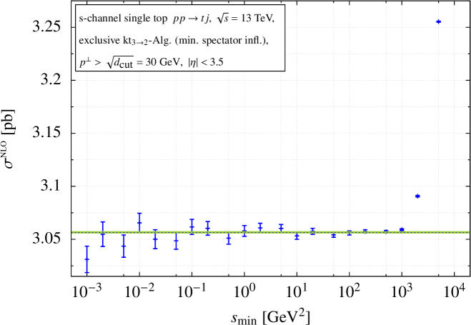
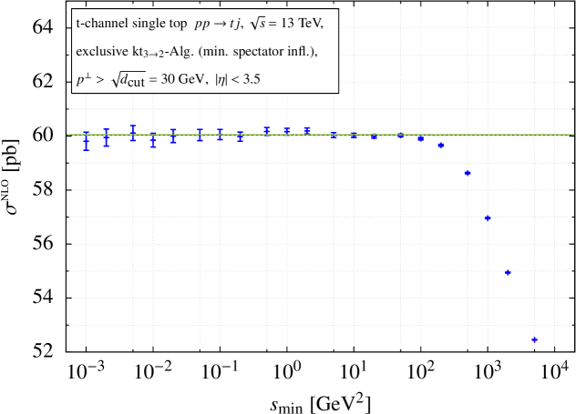
Virtual and real contributions in eq. (2.9) are individually IR divergent. Only their sum is finite for infrared-safe observables as guaranteed by the Kinoshita-Lee-Nauenberg theorem. In practical calculations, we thus need to regularise the related divergences and cancel them when combining real and virtual corrections. Following ref. [36] we employ the Phase Space Slicing Method (see also refs. [50, 51]) to achieve this cancellation. Within the Phase Space Slicing Method the phase space for the real corrections is split into regions where the squared matrix elements contains soft and collinear divergences and the remaining phase space. The latter can be integrated numerically in dimensions. Using soft and collinear approximations the unresolved contributions can be analytically integrated in a process-independent manner and the singularities can be cancelled with the ones in the virtual corrections. Note that the separation of the phase space into ‘singular’ regions and ‘finite’ regions should not interfere with the jet clustering. We employ the so-called one cut-off Phase Space Slicing Method method in the form as presented in ref. [36] with the slicing parameter , controlling the separation into singular and finite phase space regions. Since the slicing is to some extent arbitrary the result must be independent of . However, because of the soft and collinear approximations applied in the singular regions a systematic error is introduced and the result is no longer independent of the slicing parameter. Since the error scales with it can be neglected for sufficiently small . On the other hand, since singular regions and finite regions both individually depend logarithmically on —only in the sum we find the aforementioned linear dependence—the statistical error of the numerical Monte-Carlo integration grows with smaller and it takes more time to perform the numerical integration. An important test within the Phase Space Slicing Method is thus to numerically establish the approximate independence of the final results of the choice of for sufficiently small values and to find a compromise between statistical and systematic uncertainties.
Because -channel and -channel largely differ in size, we perform this analysis for each channel separately since otherwise potential problems in the -channel could hide because of the large -channel contribution. The fact that the -channel gives only a small contribution to single top-quark production which is difficult to establish experimentally makes the application of the Matrix Element Method to the -channel also particularly interesting. The Matrix Element Method might help in separating the -channel contribution from -channel production.
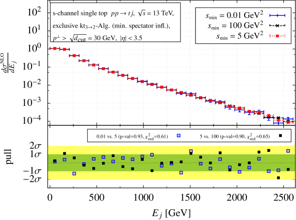
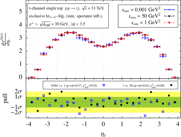
Fig. 3.1 shows the fiducial cross sections for the -channel and -channel production of single top quarks in association with a light jet at NLO accuracy as a function of the slicing parameter . For (-channel) and (-channel) fig. 3.1 shows plateaus of the fiducial cross sections compatible with constant values within the statistical errors. The straight dashed lines show the results of fits to the first (-channel) and (-channel) data points assuming constant cross sections. The fits yield pb for the -channel and pb for the -channel. Fig. 3.1 also illustrates the increasing statistical uncertainties for decreasing values. The dependence as shown in fig. 3.1 suggests to choose a value for the slicing parameter well below for the -channel and for the -channel. As a compromise between statistical and systematic uncertainties we choose for the -channel and for the -channel. Concerning the total cross sections this seems rather small given the results shown in fig. 3.1. However, differential distributions which we study next, may introduce additional scales and may be more sensitive to . In this context and seem to be a good choice since they should be well below all relevant physical scales and are still large enough to prevent large statistical fluctuations in the numerical integration. Fig. 3.2 shows distributions of the top-tagged jet and the light jet for three different values of . In the plots we show results obtained with the nominal values (-channel) and (-channel) as discussed above and results obtained for lower values of (respectively ) and higher values of (respectively ). At the bottom of each plot the difference of the results obtained with different are shown normalised to the statistical uncertainty (‘pull’). As we can see from fig. 3.2 (and various other distributions which we also checked but do not show here) any dependence of the differential distributions is at most of the order of the statistical uncertainties and thus negligible. While this conclusion is already obvious from the distribution of the pull in the lower plots, we also calculated, as a more quantitative measure, the corresponding -value and the reduced for the comparison of the histograms as described in ref. [53] and implemented in refs. [54, 55, 56]. From the results we conclude that within the uncertainties the distributions obtained for different agree with each other. The chosen values are thus sufficiently small also for differential cross sections. Note that for the aforementioned studies we used the factorised phase space parameterisation as described in section 2.3. Since this involves different parameterisations in different (singular) phase space regions, the approximate slicing-parameter independence of the differential distributions also serves as a first consistency check of their implementation.
3.1.3 Validation of the phase space parameterisation
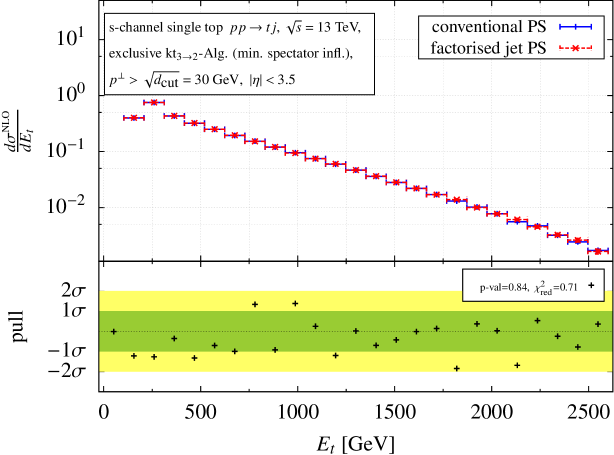
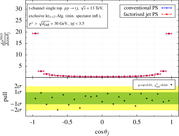
As mentioned above depending on which partons are clustered and how the spectator is chosen different phase space parameterisations are used in different phase space regions in case of the real corrections. The implementation involves some combinatorics and the coding of the formulas as presented in the appendix A and in ref. [24]. To validate the phase space parameterisation we reproduce various distributions of -jet observables at NLO accuracy that have been calculated with a conventional parton level Monte-Carlo generator in combination with the jet algorithm. Using the factorised phase space parameterisation any distribution of an -jet observable can also be calculated at NLO by integrating the differential jet cross section as defined in eq. (2.27) over the jet momenta:
| (3.7) |
Comparing the two approaches allows us to check the implementation of the phase parameterisations. In addition, the identification of the jet momenta given by the -body phase space in the factorised phase space in eq. (3.7) with the momenta of the jets obtained from the corresponding jet algorithm is checked. As examples, we study the energy distribution of the top-tagged jet for the -channel and the polar angle distribution of the light jet for the -channel in fig. 3.3. The distributions calculated using the conventional parton level Monte-Carlo generator employing the jet clustering are shown as blue lines while the ones obtained according to eq. (3.7) are shown as dashed red lines. Their difference normalised to the statistical uncertainty is shown at the bottom of each plot. In addition, we show again -value and normalised as introduced in the previous section. Since the distributions have not been normalised the cross check of the differential cross sections also serves as a validation of the fiducial cross sections. We study the exclusive case since we are especially interested in the case when real radiation is unresolved and there is a non-trivial mapping from partonic to jet momenta. (The contribution from events with an additional jet would be calculated according to the last line of eq. (2.9) and does not involve any technical or conceptual problems.)
Inspecting the plots in fig. 3.3 (and various other distributions which we also checked but do not show here) we find perfect agreement within the statistical uncertainties between the two approaches. The results for the -values and the reduced further support this interpretation.
3.2 Generation of unweighted single top-quark events distributed according to the NLO cross section
Interpreting the differential jet cross section as an event weight allows to use eq. (2.27) to generate unweighted jet events following the NLO cross sections. As described in ref. [24] we use a simple Acceptance-Rejection algorithm to unweight the NLO events. To validate this procedure, we first generate unweighted events and recalculate distributions of -jet observables that have been calculated in the previous section using the conventional parton level Monte-Carlo.
3.2.1 Exclusive event definition
Having in mind the extraction of the top-quark mass with the Matrix Element Method from our generated events, we have to specify an event definition that does not make any assumption on the top-quark mass. For example, one may use energies and angles to define the measured events in our pseudo experiment. Again, we use the clustering prescription introduced in the previous section. Because in current experiments a recombination is used, we study first the impact of the modified recombination procedure. Since the difference in the results using different recombination procedures is an NLO effect, this study provides also valuable information to minimise the impact of NLO corrections by choosing a sensible event definition. We study first the exclusive case where we demand precisely one additional light jet and veto events with more than one light jet.
Impact of the new jet clustering
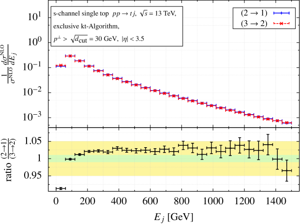
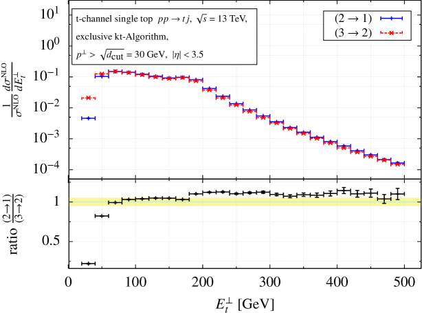
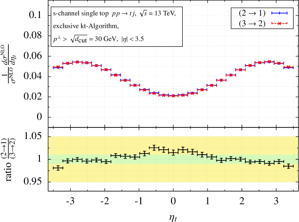
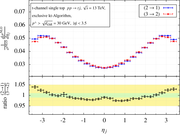
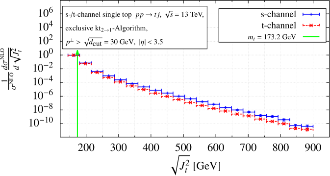
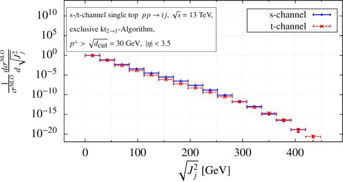
The Matrix Element Method at NLO, as described in ref. [24], is only sensitive to normalised distributions (shapes) but not to the total number of measured events. Obviously, the distributions are affected by the jet algorithm. In fig. 3.4 and fig. 3.5 (and also fig. B.1 to fig. B.6 in appendix B.1) we illustrate the impact of the modified clustering prescription as introduced in ref. [24] and reviewed in the previous section for different variables. Fig. 3.4 and fig. 3.5 (and also fig. B.1 to fig. B.6) show that in most cases the impact of the different recombination schemes is small and at the level of a few per cent only. However, there are also pronounced differences: The shapes of some energy distributions can differ up to in bins near the kinematical threshold (cf. fig. 3.4). This is easily understood by the fact that the prescription strictly keeps the jets on their mass-shell while the masses of the clustered jets can differ severely from the masses of the parent partons. This is studied in detail in fig. 3.6, where we show the mass distribution of the jet containing the top quark and the light jet for the clustering. In the clustering the distribution would be proportional to delta functions: in case of the top jet and in case of the light jet. In particular, at the phase space boundaries this can lead to significant differences, explaining the large effects in the threshold region. In addition, the clustering always maintains exact four momentum conservation and in particular transverse momentum balance also in the case of an unresolved jet.444Note that using the P-scheme where the recombined momentum is defined as the sum of the 4-momenta of the recombined particles 4-momentum conservation is also guaranteed in the recombination. However, particles close to the beam are simply dropped and not recombined. In this case the transverse moment is no longer balanced. The angular distributions do not have a pronounced mass dependence and as a consequence the corresponding differential distributions show only minor differences of a few percent in all bins (cf. fig. 3.5). It is worth mentioning that the aforementioned differences are formally due to higher orders in perturbation theory. The large differences in specific phase space regions may also signal that the NLO corrections are large in these regions and fixed order perturbation theory might become unreliable. Defining the events in terms of variables with only a weak dependence on the clustering prescription may thus also help in improving the reliability of the perturbative description of measured observables.555In all applications usually some reduction on the used variables occurs: Either because some variables are in principle unmeasurable (e. g. neutrino variables) or because the experimental accuracy is not good. The definition of events in terms of four-momenta is then accomplished from the variables by imposing certain kinematics (cf. below).
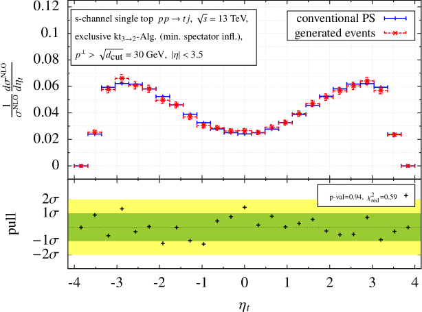

To define an exclusive single top-quark event in , we use the pseudo rapidity of the measured top-quark jet () and the energy, pseudo rapidity and azimuthal angle of the light jet (). Since the decay of the top quark is not considered in the calculation presented here, we use only the rapidity of the top quark and information related to the light jet. From fig. 3.4 and fig. 3.5 (and also fig. B.1 to fig. B.4) we conclude that for these variables the impact of the modified clustering prescription is small. The vector introduced in the previous section, collecting the hadronic variables, is thus given by . In terms of these variables the two (resolved) jet momenta read:
| (3.8a) | |||||
| (3.8b) | |||||
with
Note that the parameterisation of the jet momenta depends on the top-quark mass which occurs as a free parameter. Using
| (3.9) |
and
| (3.10) | |||||
the event weight including NLO corrections reads:
| (3.11) |
In fig. 3.7 the pseudo rapidity distribution of the top-tagged and the energy distribution of the light jet are shown for - and -channel single top-quark production at NLO. The histograms calculated using the conventional parton level Monte-Carlo with subsequent jet clustering are shown as blue lines while the ones filled by the unweighted NLO events are shown as dashed red lines. Their difference normalised to the statistical uncertainty is shown at the bottom of each plot. Again the -value and the reduced of the comparison of the two histograms are shown. Fig. 3.7 illustrates that filling the histograms with the unweighted NLO events perfectly reproduces the distributions calculated with a conventional parton level Monte-Carlo integration. Again we have also checked various other distributions which we do not show here. In all cases we find perfect agreement between the two approaches. We can thus conclude that the generation of unweighted events with NLO accuracy is successfully validated.
3.2.2 Inclusive event definition
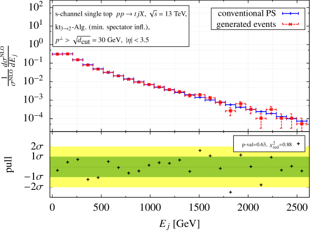
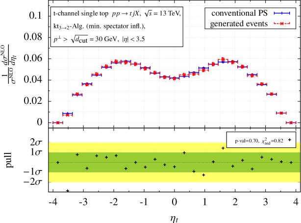
In this section we use an inclusive event definition. We study without a veto on additional jet emission. We note that in the contributions with an additional resolved jet no clustering takes place at NLO accuracy. Taking these contributions into account can therefore only improve the impact of the clustering studied in section 3.2.1 since the relative weight of clustered events is reduced. Hence, we use the same set of variables as before: the pseudo rapidity of the top-quark jet () and the energy, pseudo rapidity and azimuthal angle of the hardest light jet (): . For events with only one top-tagged jet and one light jet the same parameterisation as described in the previous section can be used. In case that an additional jet is resolved (denoted by , denotes the hardest light jet) we use
| (3.12a) | |||||
| (3.12b) | |||||
| (3.12c) | |||||
with
Since we are inclusive in the additional jet the related variables have to be integrated over the allowed range:
The boundaries follow from the definition of the inclusive event sample. For the inclusive event definition we choose the central renormalisation scale and factorisation scale on an event-by-event basis as the total transverse energy of the resolved final state:
| (3.13) |
Using again eq. (3.9) and
| (3.14) | |||||
the -jet contribution to the NLO jet event weight can be obtained from
| (3.15) | |||||
The NLO jet event weight for the inclusive event sample is the sum of the exclusive -jet contribution from eq. (3.11) and the -jet contribution defined above
| (3.16) |
Again we validate the NLO event generation by comparing differential distributions calculated using unweighted events with the distributions determined through a conventional Monte-Carlo integration. Fig. 3.8 shows results of the two approaches for - and -channel single top-quark production. As one can see from fig. 3.8 the two results are in perfect agreement with each other. We have also scrutinised the other distributions of the observables in the inclusive event definition which we do not show here. Again, we find perfect agreement between the two approaches. We thus conclude that the generation of unweighted events including NLO corrections works.
4 Application: MEM at NLO for single top-quark production
In this section we apply the Matrix Element Method including NLO corrections to a hadron collider process. As an application, we analyse the potential to measure the top-quark mass using single top-quark events. To do so, we interpret the unweighted events generated in the previous section as pseudo data and use the Matrix Element Method to extract the top-quark mass. Note that in the unweighting, the NLO event weight has been used. The simulated event sample thus incorporates the NLO corrections.
4.1 Impact of NLO corrections
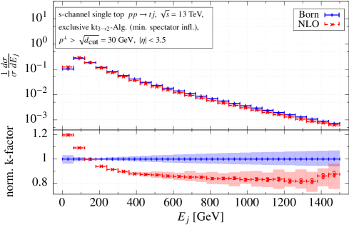
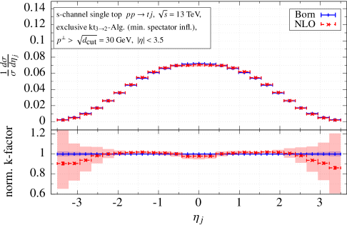
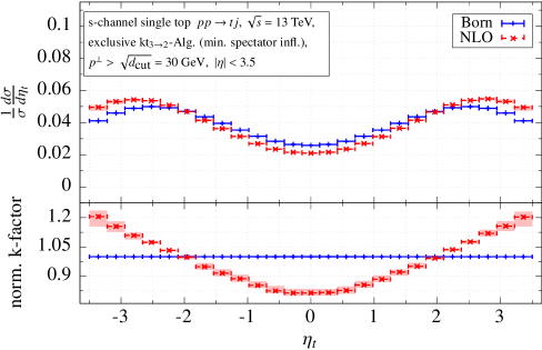
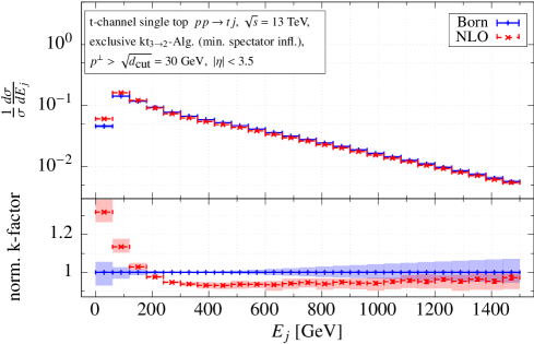
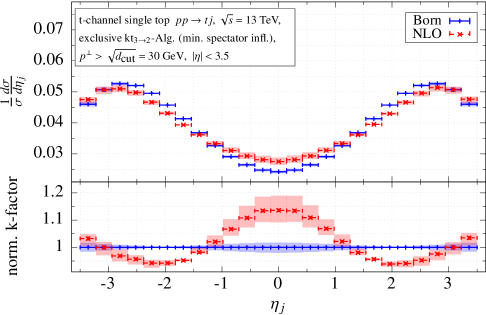
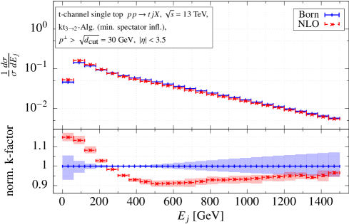
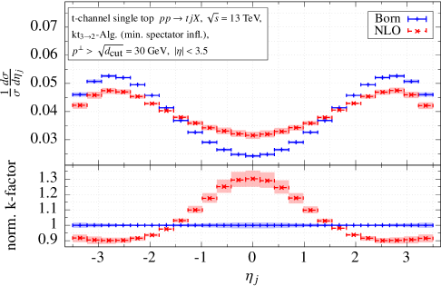
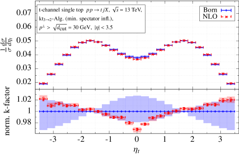
Before applying the Matrix Element Method to simulate a top-quark mass measurement it is instructive to investigate the size of the NLO corrections. Tab. 1 summarises the fiducial Born and NLO cross sections (with and without additional jet veto) for the - and -channel production of a single top quark in association with a light jet.
| -channel | -channel | |||
| excl. | incl. | excl. | incl. | |
| [pb] | ||||
| [pb] | ||||
From Tab. 1 we see that the fiducial -channel cross section with a veto on more than one light jet receives a small negative NLO correction of . The contribution of the additional jet adds to the NLO cross section. The fiducial -channel cross section with jet veto on the other hand receives a big negative NLO correction of while the contribution without jet veto reduces the size of the NLO correction to .
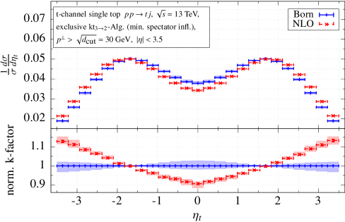
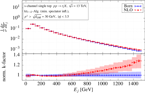
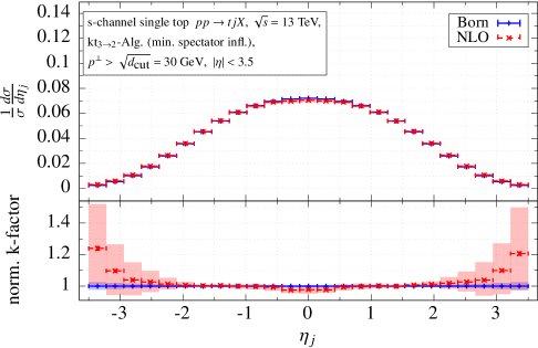
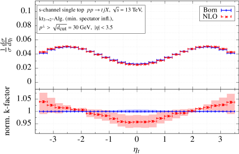
The plots in fig. 4.1 to fig. 4.4 show the impact of the
NLO corrections on the normalised differential distributions. The shaded areas show the simultaneous variation of the renormalisation
and factorisation scale between and (including
statistical errors). At the bottom the k-factors which are defined as the ratio
of the NLO results with respect to the Born results are shown. As can be seen
from fig. 4.1 and fig. 4.2, the impact of
the NLO corrections on the shapes of the -channel (-channel)
distributions ranges from to ( to ).
Varying the renormalisation and factorisation scale results in more
pronounced changes in the NLO than in the Born distributions. This is
especially true in case of the -channel for large values of the
pseudo rapidity. Note that in cases where the real corrections give
large contributions to the NLO corrections—this can happen for
example if a new partonic channel opens—the real corrections may influence
significantly the scale dependence, since this contribution is
essentially leading order and no compensation of the scale variation
takes place (see figures
4.3 and 4.4).
We conclude that the scale variation of the leading-order results does not offer a reliable estimate for the theoretical uncertainty due to missing higher-order corrections in general.
As can be seen from fig. 4.3, not
vetoing the additional resolved jet results in somewhat flatter
k-factors in regions where most of the events are
expected; except for the -channel pseudo rapidity distribution of the
light jet which receives NLO corrections of up to in the
central region.
When using the extended likelihood in the Matrix Element Method the unnormalised
distributions are relevant. For completeness they are given in fig. B.7 to fig. B.8 in appendix B.2.
4.2 Top-quark mass extraction
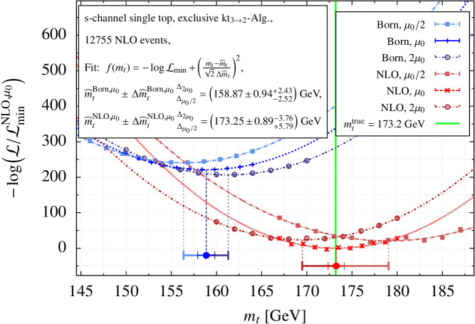
The NLO jet event weights defined in eq. (3.11) and eq. (3.16) can be used to set up likelihood functions as defined in eq. (2.6) and extended likelihood functions as defined in eq. (2.7) at NLO accuracy. Interpreting the unweighted events generated in section 3.2.1 and 3.2.2 as pseudo data, we now apply the Matrix Element Method to them. To investigate the impact of the additional -jet events on the inclusive analysis we choose the relative sizes of the even samples to reflect the fiducial cross sections (cf. table 1):
| (4.1) |
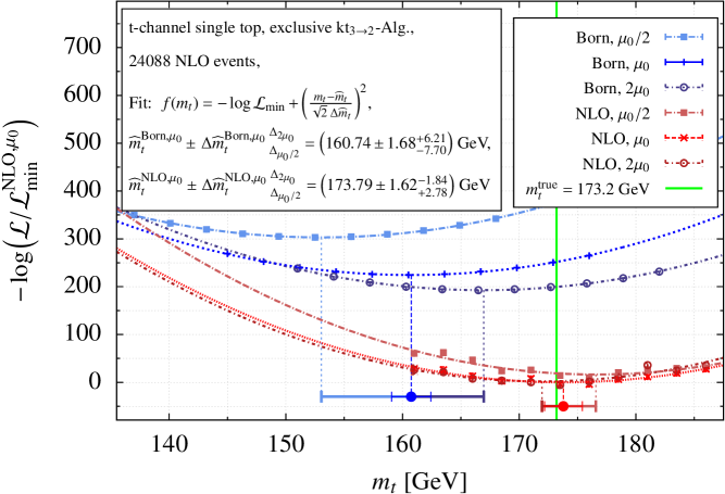
The generated samples of () NLO exclusive -channel (-channel) and () NLO inclusive -channel (-channel) single top-quark events are thus treated as results of different (toy) experiments which we analyse using the Matrix Element Method employing the respective (extended) likelihood functions. In particular, as illustration, the Matrix Element Method is used to extract the top-quark mass. This serves as a consistency check of the procedure and provides another useful check of the numerical implementation. Furthermore, the analysis can be used to estimate the potential of the Matrix Element Method applied to top-quark mass measurements including higher-order corrections. Figure 4.5 shows the negative logarithm of the likelihood (‘log-likelihood’) as a function of the top-quark mass evaluated with the sample of () exclusive NLO -channel (-channel) single top-quark events. For each event sample we calculate the negative logarithm of the likelihood for different values of the top-quark mass. The results for three different scale settings (see also eq. (3.5) for the definition of .) are shown as open-circles (), crosses () and solid squares (). The lower (red) points are obtained using NLO predictions for the event weight in the definition of the likelihood, while the upper (blue) points use the Born approximation for the event weights. The lines connecting the data points show the result of a parabola fit. The vertical line at corresponds to the true value used in the event generation. Fig. 4.5 shows that including the NLO corrections leads to significant smaller values for . The NLO predictions give thus a better description of the unweighted events. This is not a surprise as the events were generated using the NLO predictions of the cross sections. The good agreement should be seen as a consistency check of the approach. The top-quark mass is extracted as the minimum of the negative log-likelihood function. For the -channel (-channel) we obtain for an estimator () employing the NLO likelihood and () in case the LO likelihood is used. In addition, we estimate the uncertainty of the determined mass value. Repeating the mass determination using and a measure for the theoretical uncertainty is calculated from the difference with respect to the result for . The shifts for () are indicated in the legend as superscripts (subscripts ). The scale uncertainty represents a limiting factor on the reachable accuracy. In addition, we quote the statistical uncertainty of the estimator determined from the fit. The results are illustrated as data points in the lower part of the plots with the uncertainties due to the scale variation shown as thick error bars and the statistical uncertainties shown as thin error bars. While for the -channel the mass values extracted using LO, respectively NLO predictions are marginally consistent (taking into account the large scale uncertainty), we find a significant difference of about in case of the -channel, which is not covered by the scale variation.
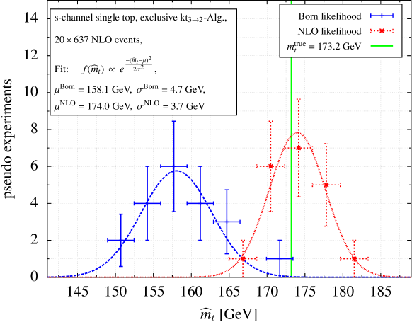
As mentioned before the Maximum Likelihood estimator is prone to introduce a bias in case the data is not well described by the assumed probability distribution. To make sure that this indeed the origin of the aforementioned discrepancy, we investigate the consistency of the procedure by splitting the data sample into subsamples, treating each subsample as an individual experiment. Binning the results based on the subsamples allows to check whether the bias is of systematic origin as suggested before or due to some statistical outliers. The result for the -channel with events per subsample is shown in fig. 4.6. As expected, including the NLO corrections in the evaluation of the event weights, fig. 4.6 shows that no bias is introduced in the estimator. In contrast, employing only the Born approximation in the calculation of the event weights, a significant bias is introduced. Fig. 4.6 illustrates that the shift observed using LO predictions is indeed a consequence of assuming the ‘wrong’ probability distribution for the event sample and not due to a statistical fluctuation, since the results of the 20 pseudo experiments give a consistent picture. We stress that this shift per se does not preclude the application of the Matrix Element Method in LO: the shift can be accounted for by an additional calibration procedure. However, since this calibration introduces additional uncertainties it is preferable make the assumed probability distribution as accurate as possible. While the occurrence of the mass shift using LO or NLO predictions is not surprising we stress that the size of the effect was never precisely quantified before. Furthermore, as mentioned above estimating the leading-order theory uncertainties using scale variation does not provide a reliable estimate of higher order effects. While the calibration may reproduce the true mass value, the uncertainty estimates would be unreliable. In particular, compared to the NLO result the uncertainties could be underestimated.
We shall also comment on the scale uncertainty observed using LO and NLO predictions. While in the -channel the uncertainty due to the scale variation is reduced when going from LO to NLO predictions, this is not the case for the -channel. Varying the scale in the likelihood used to extract the top-quark mass results in a shift of the NLO estimator between and while the Born estimator varies between and . For the -channel, the related uncertainties thus increase when going from LO to NLO, in contrast to the naive expectation. However, the LO predictions are due to electroweak interaction and the scale enters only through the factorisation scale dependence of the parton distribution functions. Furthermore, since the event weight is calculated from normalised distribution, this dependence cancels to some extent in the ratio. As a consequence, the scale variation of the leading-order result does not provide a reliable method to estimate the effect of higher-order corrections. It is thus not surprising that the picture we observe is different from the naive expectation and the uncertainties based on the LO scale variation underestimates the true uncertainty. We also point out that for -channel and -channel production the scale uncertainties dominate. The statistical uncertainties amount to GeV for -channel and GeV for the -channel (in the exclusive -channel (-channel) analysis the event sample contains only () events).
Inclusive event definition
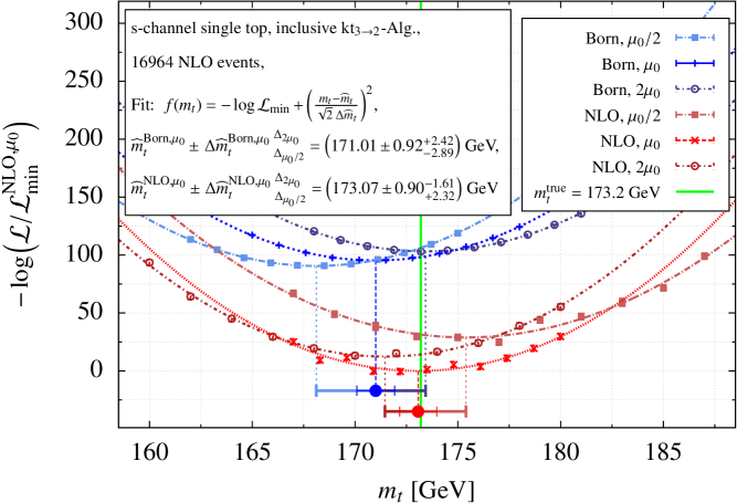
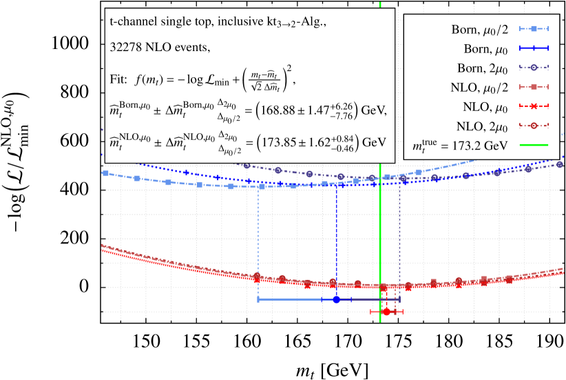
Note that vetoing additional resolved jets requires phase space cuts on the additional radiation. These cuts introduce additional scales into the NLO calculation leading to potentially uncancelled logarithms which might spoil the convergence of perturbation theory. In the inclusive event definition this veto is dropped. Fig. 4.7 shows the corresponding analysis using the inclusive event definition. In difference to the exclusive case discussed before, we observe for both production channels an improvement of the scale uncertainties when going from LO to NLO. For the -channel, the uncertainties are almost reduced by a factor of ten. In case of the -channel the improvement is less impressive. The scale variation of and for the Born estimator is reduced to and in case the NLO likelihood is used. We also note that for the inclusive event definition the difference of between the central values in LO and NLO is now well covered by the scale variation. For both production channels, we find that the extracted top-quark mass is consistent with the true value used in the event generation. While in the -channel the scale uncertainty dominates, the scale uncertainty in the -channel amounts to less than uncertainty of the extracted top-quark mass and the total uncertainty is dominated by the statistical uncertainty. The latter could be reduced using a larger event sample. We also note that the increased sample size of the inclusive events with respect to the exclusive event sample (cf. eq. (4.1)) does not result in improvements of the relative uncertainties of the analyses. As presented further down in eq. (4.2) and eq. (4.3), the inclusive cross section is slightly less sensitive to the top-quark mass which compensates the statistical gain of the larger sample sizes.
Extended likelihood
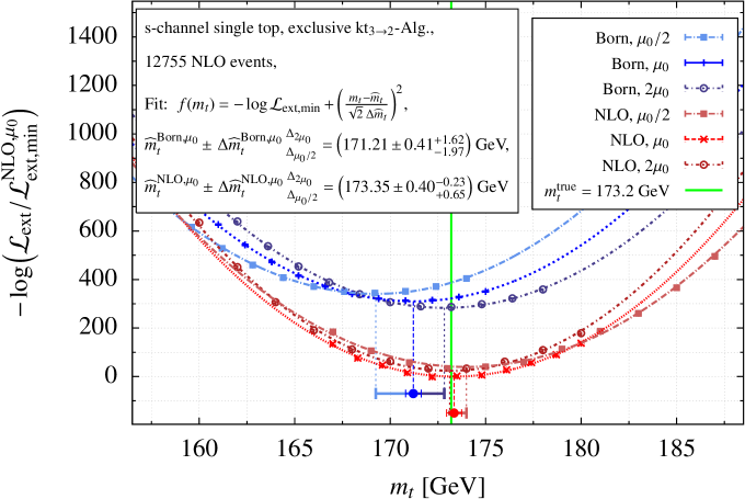
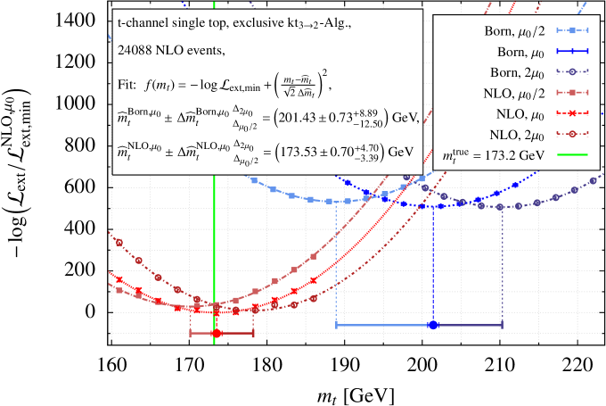
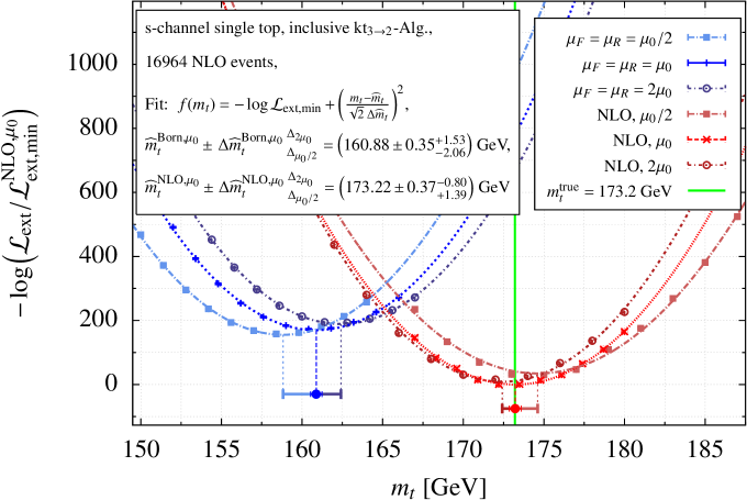
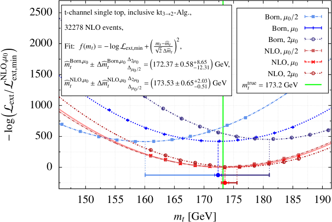
In the previous section we argued that with extended likelihoods the information contained in the total event number may be used to improve the parameter determination. Fig. 4.8 (Fig. 4.9) shows the extended log-likelihoods for -channel and -channel production using the exclusive (inclusive) event definition. As before we observe that using the NLO likelihood correctly reproduces the true mass value used in the event generation. Using the extended Born likelihood the values of the estimators are driven by two competing effects: Reproducing both the NLO distributions and the NLO fiducial cross sections using only Born predictions. When comparing the exclusive analyses presented in fig. 4.5 and fig. 4.7 with the fiducial cross sections given in table 1, the analyses based on extended likelihoods show that the impact of the expected total event numbers is dominating this compromise: In the exclusive case the fiducial -channel cross section receives only a small NLO correction which leaves little room for a shift of the top-quark mass. On the other hand, the exclusive fiducial -channel cross section receives a large negative NLO correction. Hence, the estimator extracted with the extended Born likelihood gets pushed to higher top-quark mass values in order to reduce the Born cross section accordingly. In the inclusive analysis the -jet contribution significantly increases the NLO correction to the fiducial -channel cross section. As a result, the Born estimator is pushed to smaller top-quark mass values to open up more phase space for the Born cross section. In the inclusive -channel the -jet contribution compensates the large negative exclusive NLO correction leaving only little room for a shift in the Born estimator. The shifts of the NLO and Born estimators due to scale variation in the extended likelihoods largely follow the same pattern deduced from table 1 which overall leads to a considerable reduction of the theoretical uncertainty estimates when taking NLO corrections into account. Concentrating on the statistical uncertainties, we observe a significant improvement in case the extended likelihood is used: The uncertainty is roughly reduced by a factor of two.
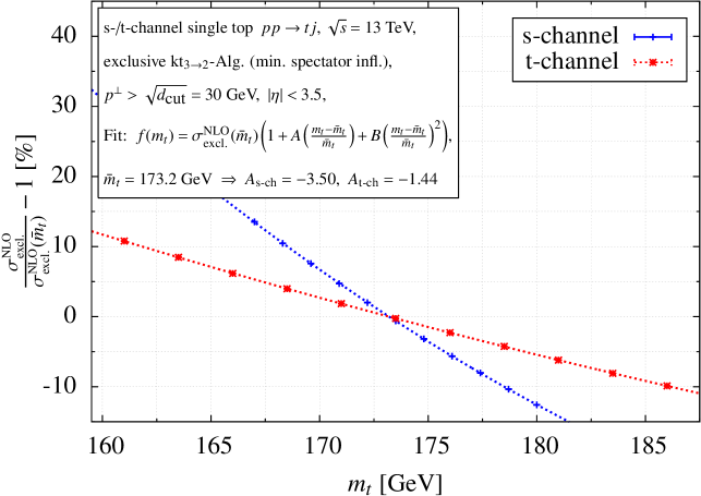

The relative uncertainty fits nicely with the naive expectation based on the assumption that the cross section will be measured with an relative uncertainty of the order where denotes the total event number: In fig. 4.10 we show the dependence of the fiducial exclusive and inclusive cross sections calculated including NLO corrections and infer the top-quark mass sensitivities by approximating the dependence of the cross section on the top-quark mass by a polynomial as presented in refs. [38, 57]. For the top-quark mass sensitivities of the fiducial exclusive cross sections this yields
| (4.2) |
The fiducial inclusive cross sections are slightly less sensitive to the mass of the top-quark
| (4.3) |
From eq. (4.2) and eq. (4.3) we can estimate the relative uncertainties of top-quark mass determinations based on idealised measurements of fiducial cross sections as
| (4.4) |
and
| (4.5) |
To estimate the impact of the information contained in the event sample sizes ( and ) we form weighted averages of the results given in eq. (4.4) and eq. (4.5) and the results of the analyses presented in fig. 4.5 and fig. 4.7 (which are only sensitive to normalised differential cross sections). We find relative uncertainties for the respective weighted averages of () in case of the exclusive -channel (-channel) and () in case of the inclusive -channel (-channel). These improved top-quark mass sensitivities achieved by this simple combination match the relative uncertainties of the extended likelihood analysis presented in fig. 4.8 and fig. 4.9. As mentioned before this gain in sensitivity should be compared with the additional systematic uncertainty due to the imperfect knowledge of the integrated luminosity. To estimate the impact of the uncertainty of the luminosity, we have repeated the analysis varying the luminosity by (see e.g. ref. [58]) . We identify the observed shifts of the extracted top-quark masses of about GeV ( GeV) for the -channel (-channel) as an additional systematic uncertainty. Because of this additional uncertainty the extended likelihood does not lead to a more precise measurement unless the uncertainty of the integrated luminosity is significantly reduced.
The results from the various analyses shown in fig. 4.5 to fig. 4.9 are summarised in table 2 and table 3. As mentioned before, using the NLO likelihood always reproduces the true mass value used in the event generation. Using instead the LO likelihood to extract the top-quark mass can lead to significant deviations from the true value. These deviations tend to be smaller for the inclusive event definition. In most cases the inclusion of the NLO corrections reduces the uncertainty related to the scale variation. However, as mentioned before, one should keep in mind that the LO prediction is a purely electroweak process and the variation of the factorisation scale alone does not give a reliable estimate of higher-order corrections. This is also reflected in the observation that for the -channel the mass values extracted from the exclusive event sample using LO and NLO predictions do not agree within the scale uncertainty.
| estimator [GeV] | |||
|---|---|---|---|
| Likelihood | NLO | ||
| Born | |||
| Extended Likelihood | NLO | ||
| Born | |||
| estimator [GeV] | |||
|---|---|---|---|
| Likelihood | NLO | ||
| Born | |||
| Extended Likelihood | NLO | ||
| Born | |||
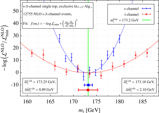
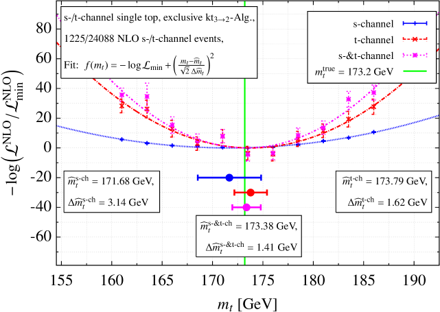
In fig. 4.11 we compare the sensitivity to the top-quark mass for - and -channel single top-quark production for a fixed number of events. The -channel shows a higher mass sensitivity leading as far as the statistical uncertainties are concerned to a more precise mass measurement assuming the same number of events. Because of the higher mass sensitivity of the -channel, the log-likelihood is significantly narrower than the log-likelihood for the -channel leading to a reduction of the statistical uncertainty by roughly a factor compared to the -channel. This factor is also consistent with the results presented for the fiducial cross sections in eq. (4.2). In practice, the higher sensitivity of the -channel is compensated by the times larger event rate of the -channel. It is thus interesting to study the impact of the -channel on a mass measurement assuming a realistic mixture of - and -channel events. Fig. 4.12 illustrates the mass measurement using an event sample with () -channel (-channel) events. As one can see in fig. 4.12 the -channel leads to a significantly smaller uncertainty in the mass extraction. The uncertainty in the -channel is roughly twice as large as in the -channel. Including both channels in the mass extraction leads to a minor improvement of the statistical uncertainty by about MeV compared to the -channel only case. This observation is again consistent with a simple weighted mean of the separate mass extractions from -channel events and -channel events yielding GeV.
5 Conclusion
In this article we have presented the first application of the MEM at NLO to the hadronic production of jets using the example of single top-quark production at the LHC.
Modifying the recombination prescription of conventional jet algorithms by using a clustering inspired by the Catani-Seymour dipole formalism allows to factorise the real phase space such that the unresolved phase space regions can be efficiently integrated numerically. Because of the clustering the clustered jet momenta satisfy four-momentum conservation and the on-shell conditions. The momenta of the resolved jets can thus be used in the virtual matrix element enabling a point-wise cancellation of IR divergences in combination with the real contribution—assuming an IR regularisation scheme has been used in intermediate steps. It is thus possible to define a fully differential event weight for jets instead of partons. As an important application the event weight can be used to generate unweighted jet events distributed according to the NLO cross section. It is also possible to attribute NLO weights to jet events observed in experiments—as needed for the MEM at NLO.
As proof of concept, we have generated events following the NLO cross section for the hadronic - and -channel production of a single top quark in association with a light jet (with an optional veto on additional jet activity). We have checked that the unweighted events reproduce the differential distributions obtained using a conventional parton level Monte-Carlo integration. As a further consistency check, the top-quark mass has been successfully reproduced from the event samples using the MEM at NLO. When extracting the top-quark mass using Born matrix elements in the MEM we find significant biases in the estimators. In particular, we observe that in general the shift is not covered by the theoretical uncertainties estimated using scale variation. While the shift could be taken into account through a calibration procedure most likely the theoretical uncertainties would be underestimated relying on LO results only. Using the Matrix Element Method at NLO accuracy might thus help in reducing the required calibration (together with the associated uncertainty) and providing a reliable estimate of the theoretical uncertainty. Furthermore, when using the Matrix Element Method at NLO accuracy the renormalisation scheme of the extracted parameters is uniquely defined.
We have applied the general algorithm presented in ref. [24] which relies on a modification of the clustering prescription to cover the most general event definitions in terms of any observables that can be constructed from the -momenta of the observed jets.
We stress that the analyses presented in this paper only present the starting point for the MEM at NLO machinery. An important aspect of this article is to serve as a proof of concept and illustrate the potential gain of using then Matrix Element Method at NLO accuracy. Further studies are required to describe more realistic final states: While the inclusion of the top-quark decay in the calculation of the likelihood should be conceptually straightforward more work is needed to incorporate also the effect of a parton shower. (The possibility to combine the approach pursued in refs. [19, 20] with the MEM at NLO framework presented here could for example be investigated.) For more complicated processes the Phase Space Slicing Method used in this article to cancel the IR singularities, should be replaced by a subtraction type method. As already stated in section 2.1, considering non-trivial transfer functions in the framework of the Matrix Element Method at NLO accuracy might require careful studies and dedicated research on its own. With all that in mind, let us point out that the performance of the Matrix Element Method at NLO and LO accuracy should ultimately be compared in the application to events that mimic realistic outcomes of experiments as closely as possible to get the best estimate on what would happen with real data. Nevertheless, despite some limitations the studies presented in this work illustrate that missing higher-order corrections in the theoretical predictions might not only introduce biases in the extracted estimators but may also render the inferred systematic uncertainty estimates unreliable. Under the assumption that fixed-order NLO calculations give a better approximation of real data than LO ones, we expect these effects to play a role in the experimental application of the Matrix Element Method as well. For future studies it will be worthwhile to repeat the corresponding analyses with events obtained from an independent, state-of-the-art NLO event generator with a parton shower that can be tuned to data like e.g. POWHEG (see ref. [59]) or MG5aMC@NLO (see ref. [60]). This will allow to further quantify whether effects of similar size to the above findings are also to be expected in parameter extractions when the method is applied to real data.
Acknowledgements
We would like to thank Markus Schulze for his careful reading of the manuscript and his valuable comments. We acknowledge useful discussions with our colleagues of the ATLAS collaboration, in particular: Patrick Rieck, Sören Stamm and Oliver Kind. This work is supported by the German Federal Ministry for Education and Research (grant 05H15KHCAA).
Appendix A Phase space parameterisation adapted to the Phase Space Slicing Method
A.1 Final-state clustering with final-state spectator
For massive partons , , the phase space can be factorised in terms of a phase space of jets and the dipole phase space measure related to the clustered parton:
| (A.1) |
When employing the Phase Space Slicing Method it is useful to express the integration via the invariants
| (A.2) |
with
| (A.3) |
and
| (A.4) |
as
| (A.5) | |||||
The Källén function is defined as
| (A.6) |
The integration boundaries read
with the relative velocities between and or given by
The phase space parameterisation corresponds to the following clustering of partons to jets
| (A.7) |
which fulfil momentum conservation () and the on-shell conditions ( for ).
The inversion of the clustering is the same as in ref. [24] with and as defined above.
In a clustering the clustering of two partons would be achieved by summing the two momenta while leaving all other momenta untouched. The difference between the clustering and the clustering as defined in eq. (2.19) can be expressed as
| (A.8) | |||||
For a given unresolved final state pair the spectator might be chosen such that it minimises given above.
A.2 Final-state clustering with initial-state spectator
The phase space of massive partons can be expressed as a phase space of particles convoluted with the dipole phase space :
| (A.9) |
Using the Phase Space Slicing Method it is again useful to use a slightly different parameterisation compared to what has been used in ref. [24]. We use the invariants
| (A.10) |
with
| (A.11) |
and
| (A.12) |
The phase space measure (after convolution with the PDFs and the flux factor) is given by
The integration boundaries read
The phase space parameterisation corresponds to the clustering of partons to jets
| (A.14) | |||||
| (A.15) |
which fulfils momentum conservation () and the on-shell conditions ( and for .).
The inversion of the clustering is the same as in ref. [24] with and as defined above.
A.3 Initial-state clustering with final-state spectator
The phase space of massive and one massless parton can be expressed as a convolution of the phase space of massive jets and the dipole phase space for the emission of an additional massless parton from the initial state with a massive final-state spectator. All statements from section A.2 can be carried over by the replacements and , and (see also ref. [24]).
The phase space parameterisation corresponds to the clustering of partons to jets
| (A.17) |
which fulfils momentum conservation () and the on-shell conditions (, ).
In a clustering the unresolved additional radiation associated with the beam would be removed from the list of momenta without changing the other final-state momenta. So the difference between the clustering defined in eq. (2.20) and the clustering can be expressed as (see eq. (A.3))
| (A.18) |
For a given unresolved final state parton the beam particle and the spectator might be chosen such that given above is minimised.
A.4 Initial-state clustering with initial-state spectator
In case of initial-state clustering with an initial-state spectator the phase space can again be written as a convolution :
| (A.19) |
When employing a Phase Space Slicing Method it is useful to express the integration after convolution with the PDFs and the flux factor via the invariants
| (A.20) |
with
| (A.21) |
and
| (A.22) |
The phase space measure (after convolution with the PDFs and the flux factor) is given by
| (A.23) | |||||
The integration boundaries read
The phase space parameterisation corresponds to the following clustering of (massless/massive) partons to (massless/massive) jets:
| (A.24) |
with
| (A.25) |
and the Lorentz boost transforming into given by
| (A.26) |
The inverse boost is obtained by exchanging and . All outgoing momenta are transformed to balance the transverse momentum. Momentum conservation () and on-shell conditions (, ) are not affected by the boost.
The inversion of the clustering is the same as in ref. [24] with and as defined above.
The sum of the jet momenta in this clustering is given by
| (A.27) |
while the sum of the partonic momenta is given by
| (A.28) |
From eq. (A.24) the influence of the clustering with respect to the clustering defined in eq. (2.20) follows as
| (A.29) |
For a given unresolved final state parton the beam particle and the spectator might be chosen such that given above is minimised.
Appendix B Additional figures
B.1 Comparison of and clustering
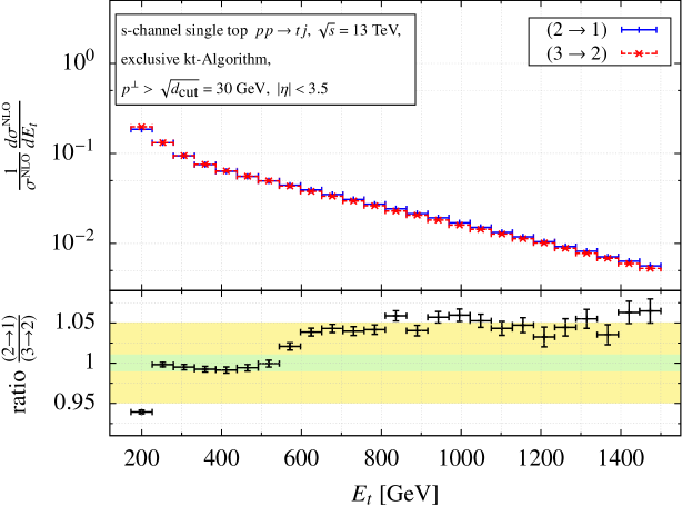
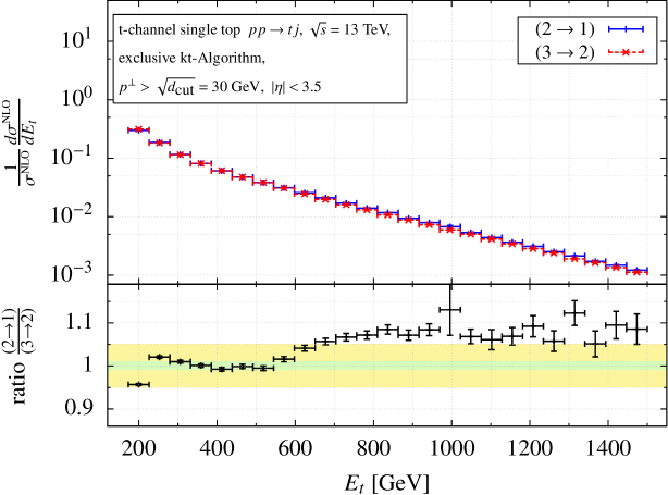
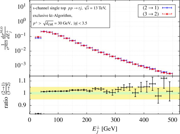
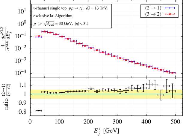
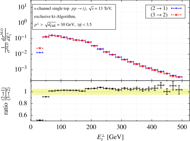
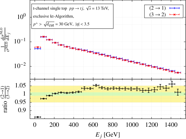
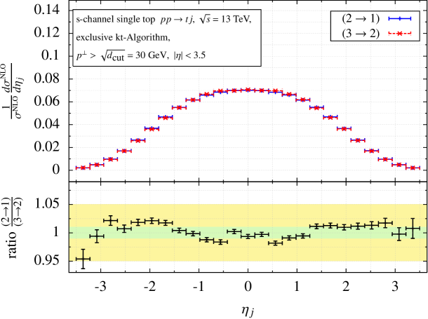
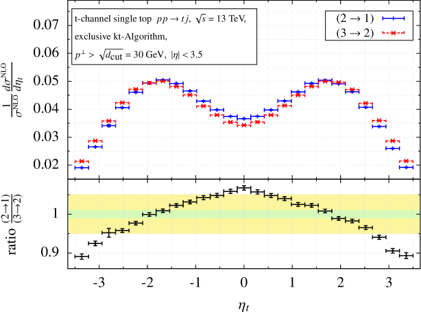
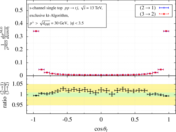
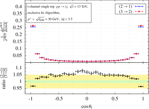
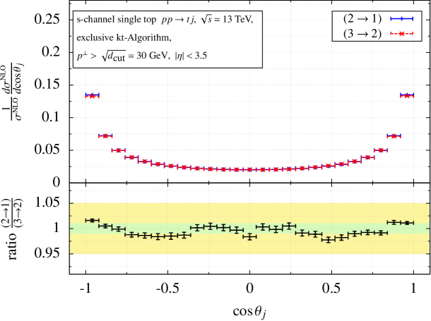
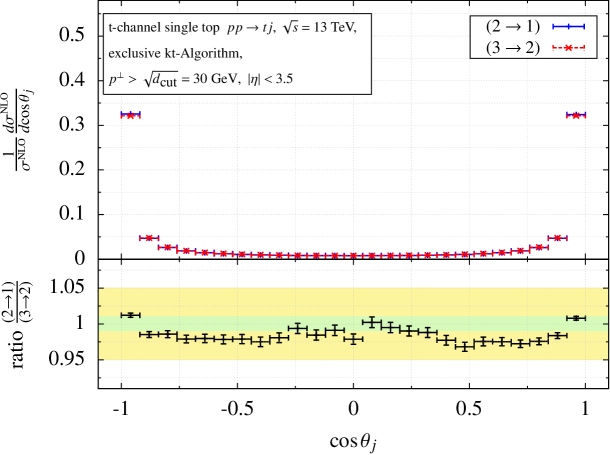
B.2 NLO corrections to differential distributions and k-factors
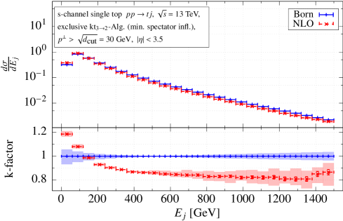
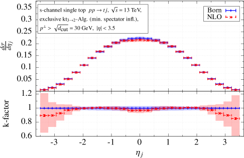
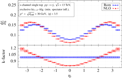
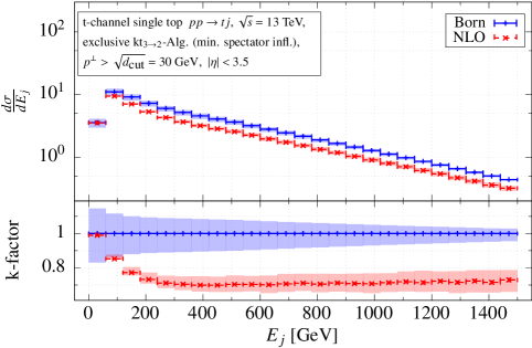
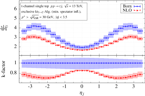
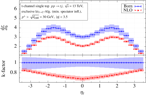
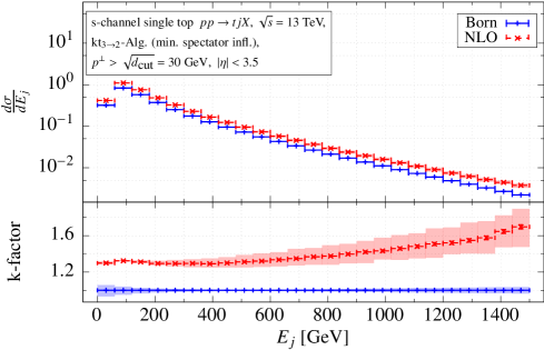
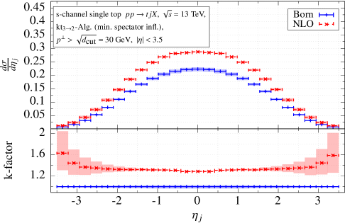
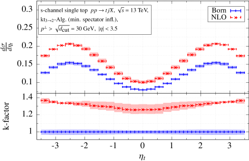
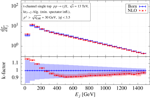
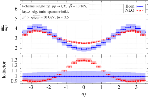
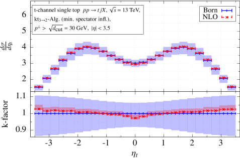
References
- [1] K. Kondo, Dynamical Likelihood Method for Reconstruction of Events With Missing Momentum. 1: Method and Toy Models, J. Phys. Soc. Jap. 57 (1988) 4126–4140.
- [2] K. Kondo, Dynamical likelihood method for reconstruction of events with missing momentum. 2: Mass spectra for processes, J. Phys. Soc. Jap. 60 (1991) 836–844.
- [3] D0 Collaboration, B. Abbott et al., Measurement of the Top Quark Mass in the Dilepton Channel, Phys. Rev. D60 (1999) 052001, [hep-ex/9808029].
- [4] D0 Collaboration, V. M. Abazov et al., A precision measurement of the mass of the top quark, Nature 429 (2004) 638–642, [hep-ex/0406031].
- [5] CDF Collaboration, A. Abulencia et al., Top quark mass measurement from dilepton events at CDF II with the matrix-element method, Phys. Rev. D74 (2006) 032009, [hep-ex/0605118].
- [6] F. Fiedler, A. Grohsjean, P. Haefner, and P. Schieferdecker, The Matrix Element Method and its Application in Measurements of the Top Quark Mass, Nucl. Instrum. Meth. A624 (2010) 203–218, [arXiv:1003.1316].
- [7] A. Giammanco and R. Schwienhorst, Single top-quark production at the Tevatron and the LHC, arXiv:1710.10699.
- [8] D. E. Ferreira de Lima, O. Mattelaer, and M. Spannowsky, Reconstructing the invisible with matrix elements, arXiv:1712.03266.
- [9] A. V. Gritsan, R. Röntsch, M. Schulze, and M. Xiao, Constraining anomalous Higgs boson couplings to the heavy flavor fermions using matrix element techniques, Phys. Rev. D94 (2016), no. 5 055023, [arXiv:1606.03107].
- [10] C. Englert, O. Mattelaer, and M. Spannowsky, Measuring the Higgs-bottom coupling in weak boson fusion, Phys. Lett. B756 (2016) 103–108, [arXiv:1512.03429].
- [11] ATLAS Collaboration, G. Aad et al., Evidence for single top-quark production in the -channel in proton-proton collisions at 8 TeV with the ATLAS detector using the Matrix Element Method, Phys. Lett. B756 (2016) 228–246, [arXiv:1511.05980].
- [12] CMS Collaboration, V. Khachatryan et al., Search for a Standard Model Higgs Boson Produced in Association with a Top-Quark Pair and Decaying to Bottom Quarks Using a Matrix Element Method, Eur. Phys. J. C75 (2015), no. 6 251, [arXiv:1502.02485].
- [13] P. Artoisenet, P. de Aquino, F. Maltoni, and O. Mattelaer, Unravelling via the Matrix Element Method, Phys. Rev. Lett. 111 (2013), no. 9 091802, [arXiv:1304.6414].
- [14] P. Artoisenet et al., A framework for Higgs characterisation, JHEP 11 (2013) 043, [arXiv:1306.6464].
- [15] I. Anderson et al., Constraining anomalous HVV interactions at proton and lepton colliders, Phys. Rev. D89 (2014), no. 3 035007, [arXiv:1309.4819].
- [16] J. R. Andersen, C. Englert, and M. Spannowsky, Extracting precise Higgs couplings by using the matrix element method, Phys. Rev. D87 (2013), no. 1 015019, [arXiv:1211.3011].
- [17] P. Artoisenet, V. Lemaitre, F. Maltoni, and O. Mattelaer, Automation of the matrix element reweighting method, JHEP 12 (2010) 068, [arXiv:1007.3300].
- [18] J. Alwall, A. Freitas, and O. Mattelaer, The Matrix Element Method and QCD Radiation, Phys. Rev. D83 (2011) 074010, [arXiv:1010.2263].
- [19] D. E. Soper and M. Spannowsky, Finding physics signals with shower deconstruction, Phys. Rev. D84 (2011) 074002, [arXiv:1102.3480].
- [20] D. E. Soper and M. Spannowsky, Finding physics signals with event deconstruction, Phys. Rev. D89 (2014), no. 9 094005, [arXiv:1402.1189].
- [21] J. M. Campbell, W. T. Giele, and C. Williams, The Matrix Element Method at Next-to-Leading Order, JHEP 11 (2012) 043, [arXiv:1204.4424].
- [22] J. M. Campbell, R. K. Ellis, W. T. Giele, and C. Williams, Finding the Higgs boson in decays to using the matrix element method at Next-to-Leading Order, Phys. Rev. D87 (2013), no. 7 073005, [arXiv:1301.7086].
- [23] C. Williams, J. M. Campbell, and W. T. Giele, Event-by-event weighting at next-to-leading order, PoS RADCOR2013 (2013) 037, [arXiv:1311.5811].
- [24] T. Martini and P. Uwer, Extending the Matrix Element Method beyond the Born approximation: Calculating event weights at next-to-leading order accuracy, JHEP 09 (2015) 083, [arXiv:1506.08798].
- [25] R. Baumeister and S. Weinzierl, Matrix element method at next-to-leading order for arbitrary jet algorithms, Phys. Rev. D95 (2017), no. 3 036019, [arXiv:1612.07252].
- [26] CMS Collaboration, S. Chatrchyan et al., Measurement of the single-top-quark -channel cross section in collisions at TeV, JHEP 12 (2012) 035, [arXiv:1209.4533].
- [27] ATLAS Collaboration, G. Aad et al., Comprehensive measurements of -channel single top-quark production cross sections at TeV with the ATLAS detector, Phys. Rev. D90 (2014), no. 11 112006, [arXiv:1406.7844].
- [28] CMS Collaboration, V. Khachatryan et al., Measurement of the t-channel single-top-quark production cross section and of the CKM matrix element in pp collisions at = 8 TeV, JHEP 06 (2014) 090, [arXiv:1403.7366].
- [29] Measurement of the Inclusive and Fiducial Cross-Section of Single Top-Quark -Channel Events in Collisions at = 8 TeV, Tech. Rep. ATLAS-CONF-2014-007, CERN, Geneva, Mar, 2014.
- [30] CMS Collaboration, A. M. Sirunyan et al., Cross section measurement of -channel single top quark production in pp collisions at 13 TeV, Phys. Lett. B772 (2017) 752–776, [arXiv:1610.00678].
- [31] ATLAS Collaboration, M. Aaboud et al., Measurement of the inclusive cross-sections of single top-quark and top-antiquark -channel production in collisions at = 13 TeV with the ATLAS detector, JHEP 04 (2017) 086, [arXiv:1609.03920].
- [32] CMS Collaboration Collaboration, Fiducial t channel single top-quark cross section at 8 TeV, Tech. Rep. CMS-PAS-TOP-15-007, CERN, Geneva, 2015.
- [33] CMS Collaboration Collaboration, Single top t-channel differential cross section at 8 TeV, Tech. Rep. CMS-PAS-TOP-14-004, CERN, Geneva, 2014.
- [34] CMS Collaboration Collaboration, Measurement of the differential cross section for -channel single-top-quark production at , Tech. Rep. CMS-PAS-TOP-16-004, CERN, Geneva, 2016.
- [35] B. Harris, E. Laenen, L. Phaf, Z. Sullivan, and S. Weinzierl, The Fully differential single top quark cross-section in next to leading order QCD, Phys.Rev. D66 (2002) 054024, [hep-ph/0207055].
- [36] Q.-H. Cao and C.-P. Yuan, Single top quark production and decay at next-to-leading order in hadron collision, Phys. Rev. D71 (2005) 054022, [hep-ph/0408180].
- [37] J. M. Campbell and R. K. Ellis, MCFM for the Tevatron and the LHC, Nucl. Phys. Proc. Suppl. 205-206 (2010) 10–15, [arXiv:1007.3492].
- [38] P. Kant, O. M. Kind, T. Kintscher, T. Lohse, T. Martini, S. Mölbitz, P. Rieck, and P. Uwer, HatHor for single top-quark production: Updated predictions and uncertainty estimates for single top-quark production in hadronic collisions, Comput. Phys. Commun. 191 (2015) 74–89, [arXiv:1406.4403].
- [39] K. Cranmer and T. Plehn, Maximum significance at the LHC and Higgs decays to muons, Eur. Phys. J. C51 (2007) 415–420, [hep-ph/0605268].
- [40] R. J. Barlow, Extended maximum likelihood, Nucl. Instrum. Meth. A297 (1990) 496–506.
- [41] G. Cowan, Statistical data analysis. Oxford University Press, 1998.
- [42] S. Catani and M. Seymour, A General algorithm for calculating jet cross-sections in NLO QCD, Nucl.Phys. B485 (1997) 291–419, [hep-ph/9605323].
- [43] S. Catani, S. Dittmaier, M. H. Seymour, and Z. Trocsanyi, The Dipole formalism for next-to-leading order QCD calculations with massive partons, Nucl.Phys. B627 (2002) 189–265, [hep-ph/0201036].
- [44] S. Frixione, Z. Kunszt, and A. Signer, Three jet cross-sections to next-to-leading order, Nucl. Phys. B467 (1996) 399–442, [hep-ph/9512328].
- [45] S. Frixione, A General approach to jet cross-sections in QCD, Nucl. Phys. B507 (1997) 295–314, [hep-ph/9706545].
- [46] S. Catani, Y. L. Dokshitzer, M. H. Seymour, and B. R. Webber, Longitudinally invariant clustering algorithms for hadron hadron collisions, Nucl. Phys. B406 (1993) 187–224.
- [47] M. Cacciari, G. P. Salam, and G. Soyez, The Anti-k(t) jet clustering algorithm, JHEP 04 (2008) 063, [arXiv:0802.1189].
- [48] M. Cacciari, G. P. Salam, and G. Soyez, FastJet User Manual, Eur. Phys. J. C72 (2012) 1896, [arXiv:1111.6097].
- [49] G. P. Salam, Towards Jetography, Eur. Phys. J. C67 (2010) 637–686, [arXiv:0906.1833].
- [50] W. T. Giele and E. W. N. Glover, Higher order corrections to jet cross-sections in e+ e- annihilation, Phys. Rev. D46 (1992) 1980–2010.
- [51] W. T. Giele, E. W. N. Glover, and D. A. Kosower, Higher order corrections to jet cross-sections in hadron colliders, Nucl. Phys. B403 (1993) 633–670, [hep-ph/9302225].
- [52] A. Martin, W. Stirling, R. Thorne, and G. Watt, Parton distributions for the LHC, Eur.Phys.J. C63 (2009) 189–285, [arXiv:0901.0002].
- [53] N. D. Gagunashvili, Pearson’s chi-square test modifications for comparison of unweighted and weighted histograms and two weighted histograms, PoS ACAT (2007) 060.
- [54] R. Brun and F. Rademakers, ROOT: An object oriented data analysis framework, Nucl. Instrum. Meth. A389 (1997) 81–86.
- [55] I. Antcheva et al., ROOT: A C++ framework for petabyte data storage, statistical analysis and visualization, Comput. Phys. Commun. 180 (2009) 2499–2512, [arXiv:1508.07749].
- [56] L. Moneta, I. Antcheva, and R. Brun, Recent developments of the ROOT mathematical and statistical software, J. Phys. Conf. Ser. 119 (2008) 042023.
- [57] J. M. Campbell, R. Frederix, F. Maltoni, and F. Tramontano, NLO predictions for t-channel production of single top and fourth generation quarks at hadron colliders, JHEP 10 (2009) 042, [arXiv:0907.3933].
- [58] ATLAS Collaboration, M. Aaboud et al., Luminosity determination in pp collisions at = 8 TeV using the ATLAS detector at the LHC, Eur. Phys. J. C76 (2016), no. 12 653, [arXiv:1608.03953].
- [59] S. Frixione, P. Nason, and C. Oleari, Matching NLO QCD computations with Parton Shower simulations: the POWHEG method, JHEP 11 (2007) 070, [arXiv:0709.2092].
- [60] J. Alwall, R. Frederix, S. Frixione, V. Hirschi, F. Maltoni, O. Mattelaer, H. S. Shao, T. Stelzer, P. Torrielli, and M. Zaro, The automated computation of tree-level and next-to-leading order differential cross sections, and their matching to parton shower simulations, JHEP 07 (2014) 079, [arXiv:1405.0301].