A new holographic dark energy model in Brans-Dicke theory with logarithmic scalar field

Abstract

We study a holographic dark energy model in the framework of Brans-Dicke (BD) theory with taking into account the interaction between dark matter and holographic dark energy. We use the recent observational data sets, namely SN Ia compressed Joint Light-Analysis(cJLA) compilation, Baryon Acoustic Oscillations (BAO) from BOSS DR12 and the Cosmic Microwave Background (CMB) of Planck 2015. After calculating the evolution of the equation of state as well as the deceleration parameters, we find that with a logarithmic form for the BD scalar field the phantom crossing can be achieved in the late time of cosmic evolution. Unlike the conventional theory of holographic dark energy in standard cosmology ($\omega_{D}=0$), our model results a late time accelerated expansion. It is also shown that the cosmic coincidence problem may be resolved in the proposed model. We execute the statefinder and Om diagnostic tools and demonstrate that interaction term does not play a significant role. Based on the observational data sets used in this paper it seems that the best value with $1\sigma$ and $2\sigma$ confidence interval are $\Omega_{m}=0.268^{+0.008~{}+0.010}_{-0.007~{}-0.009}$, $\alpha=3.361^{+0.332~{}+0.483}_{-0.401~{}-0.522}$, $\beta=5.560^{+0.541~{}+0.780}_{-0.510~{}-0.729}$, $c=0.777^{+0.023~{}+0.029}_{-0.017~{}-0.023}$ and $b^{2}=0.045$, according to which we find that the proposed model in the presence of interaction is compatible with the recent observational data.
Keywords: Holographic dark energy; Brans-Dicke theory; Coincidence problem
PACS numbers: 95.36.+x, 95.35.+d, 98.80.-k

1 Introduction

Nowadays it is strongly believed that some exotic matter with negative pressure, usually called dark energy (DE), is responsible for the accelerated expansion of our universe. Although so far lots of models have been proposed for dark energy, but it still remains one of the open issues in cosmology [1]. Among these models, the holographic dark energy (HDE) has attracted much attention in recent years [2]. This proposal is based on the holographic principle according to which all of the information saved in a certain region of space can be extracted from its boundary area and are limited by an IR cutoff [3]. It can be shown that the energy density of HDE is related to the cutoff, $L$, as $\rho_{D}=3c^{2}M_{p}^{2}/L^{2}$ [4]. Recalling that the black hole entropy (and thus its information) is also related to its horizon area (say $L^{2}$), it seems that the models of HDE are like the black hole physics and modifications of black hole laws due to for instance, modified and quantum gravity will affect the energy density of HDE and so new cosmological consequences may arise from it.

In this paper, we are going to study a HDE model in the context of BD theory of gravity and by using of the combination of recent observational data sets (SN Ia + BAO + CMB) we fix the relevant free parameters. To do this, we will choose a logarithmic form for the BD scalar field [5] which its aim is to check better agreement with observations and for the energy density of HDE we will take the form which have been proposed in [6]. In the presented model, we deal with the recent accelerated expansion and some other problems associated with the DE models like cosmic coincidence problem in a flat FRW geometry. We also investigate the differences between interacting and non-interacting modes and their relation to resolve the coincidence problem.

2 The model

Let us start with the BD gravity theory characterized with the action

$$S=\int d^{4}x{\sqrt{-g}\Big{[}\frac{1}{2}\big{(}-\phi R+\frac{w}{\phi}g^{\mu\nu}\partial_{\mu}\phi\partial_{\nu}\phi\big{)}+L_{m}\Big{]}},$$ (1)

where $R$ is the Ricci scalar, $w$ is the BD parameter, $\phi$ is the BD scalar field and $L_{m}$ denotes the matter Lagrangian density. We assume a homogeneous and isotropic FRW universe which is described by the line element

$$ds^{2}=-dt^{2}+a^{2}(t)\left(\frac{dr^{2}}{1-kr^{2}}+r^{2}d\Omega^{2}\right),$$ (2)

where $k=0,\pm 1$ and $a(t)$ are the curvature index and scale factor respectively. For a flat universe ($k=0$) the above action leads the following equations of motion

$$\frac{3}{4w}\phi^{2}H^{2}-\frac{\dot{\phi}^{2}}{2}+\frac{3}{2w}H\dot{\phi}\phi=\rho_{m}+\rho_{D},$$ (3)

$$\frac{-\phi^{2}}{4w}\left(\frac{2\ddot{a}}{a}+H^{2}\right)-\frac{1}{w}H\dot{\phi}\phi-\frac{1}{2w}\ddot{\phi}\phi-\frac{\dot{\phi}^{2}}{2}\left(1+\frac{1}{w}\right)=p_{D},$$ (4)

$$\ddot{\phi}+3H\dot{\phi}-\frac{3}{2w}\left(\frac{\ddot{a}}{a}+H^{2}\right)\phi=0,$$ (5)

where $\rho_{D}$ and $\rho_{m}$ are the energy densities of DE and dark matter (DM) respectively, $p_{D}$ is the pressure of DE and $H=\dot{a}/a$ is the Hubble function. As in [5], we assume a logarithmic relation between BD scalar field and scale factor which is claimed that it may avoid a constant result for the deceleration parameter:

$$\phi=\phi_{0}\ln(\alpha+\beta a),$$ (6)

where $\phi_{0}$, $\alpha>1$ and $\beta>0$ are some constants. In [6] a new model of HDE is proposed which is based on the DGP braneworld theory. In such a extra dimensional cosmology the four-dimensional FRW universe is embedded as a brane in a five-dimensional flat (Minkowski) bulk. The motivations to add the DE to this model is studied in [7] and by adding DE to DGP in [6] a new modified model of HDE is resulted according to which we can write the energy density of HDE as

$$\rho_{D}=\frac{3c^{2}\phi^{2}}{4wL^{2}}(1-\frac{\epsilon L}{3r_{c}}),$$ (7)

where $r_{c}=\frac{M^{2}_{p}}{2M^{3}_{5}}=\frac{G_{5}}{2G_{4}}$ stands for the crossover length scale, $\epsilon=\pm 1$ corresponds to the two branches (self-accelerated and normal) of solution [8] and $L=H^{-1}$ is the Hubble horizon as the system’s IR cutoff. The $\epsilon=+1$ is related to the self-accelerating solution in which the universe may enter an accelerating phase in the late time without additional dark energy component. When $L\ll 3r_{c}$, above equation reduces to usual HDE density. In what follows, by this choice for the system’s IR cutoff and fitting the free parameters by use of the latest observational data, we study the evolution of DE density, equation of state (EoS), deceleration parameters, ratio of DE density to density of total matter of the universe and apply diagnostic tools to find characteristics of the model.

3 Interacting model

In the presence of non-gravitational interaction between DE and DM the continuity equations can be written as

$$\dot{\rho}_{m}+3H\rho_{m}=Q,$$ (8)

$$\dot{\rho}_{D}+3H(1+\omega_{D})\rho_{D}=-Q.$$ (9)

where $\omega_{D}=\frac{p_{D}}{\rho_{D}}$ is the EoS parameter of DE. We define the dimensionless density parameters as

$$\Omega_{m}=\frac{4w\rho_{m}}{3\phi^{2}H^{2}},$$ (10)

$$\Omega_{D}=c^{2}(1-\frac{\epsilon}{3Hr_{c}}),$$ (11)

where $r_{c}=\frac{1}{4H^{2}\Omega_{r_{c}}}$. With $L=H^{-1}$ and using (6) the time derivative of equation (7) results

$$\dot{\rho}_{D}=\rho_{D}\left(\frac{\dot{\phi}}{\phi}+2\frac{\dot{H}}{H}\right)+2c^{2}\epsilon\phi\sqrt{\Omega_{r_{c}}}\dot{H}{H}.$$ (12)

The behavior of interaction with different $Q$-terms have been studied in [10]. In this work we take a simple interaction term as $Q=3b^{2}H\rho_{D}$, by use of which and with the help of equations (6), (7), (10), (11) and (8) we obtain

$$\frac{\dot{H}}{H^{2}}=\frac{\frac{\beta a}{(\alpha+\beta a)\ln(\alpha+\beta a)}\Omega_{D}-\frac{\beta^{3}a^{3}}{(\alpha+\beta a)^{3}(\ln(\alpha+\beta a))^{2}}+\frac{\beta^{2}a^{2}}{(\alpha+\beta a)^{2}\ln(\alpha+\beta a)}-2\frac{\beta a}{(\alpha+\beta a)\ln(\alpha+\beta a)}+\frac{3}{2}(\Omega_{D}(b^{2}+1)-1)}{1-\frac{\beta^{2}a^{2}}{(\alpha+\beta a)^{2}(\ln(\alpha+\beta a))^{2}}+2\frac{\beta a}{(\alpha+\beta a)\ln(\alpha+\beta a)}-\frac{1}{2}(c^{2}+\Omega_{D})}.$$ (13)

Taking time derivative of equation (11) we obtain

$$\dot{\Omega}_{D}=\frac{2}{3}\epsilon c^{2}\sqrt{\Omega_{r_{c}}}\frac{\dot{H}}{H}.$$ (14)

In order to see how the density parameter of HDE evolves, we define $\Omega^{\prime}_{D}=\frac{\dot{\Omega}_{D}}{H}$, where the prime denotes derivative with respect to $x=\ln a$. Then from equation (13) and (14) we have

$$\Omega^{\prime}_{D}=(c^{2}-\Omega_{D})\frac{\frac{\beta a}{(\alpha+\beta a)\ln(\alpha+\beta a)}(\Omega_{D}-2)-\frac{\beta^{3}a^{3}}{(\alpha+\beta a)^{3}(\ln(\alpha+\beta a))^{2}}+\frac{\beta^{2}a^{2}}{(\alpha+\beta a)^{2}\ln(\alpha+\beta a)}+\frac{3}{2}(\Omega_{D}(b^{2}+1)-1)}{1-\frac{\beta^{2}a^{2}}{(\alpha+\beta a)^{2}(\ln(\alpha+\beta a))^{2}}+2\frac{\beta a}{(\alpha+\beta a)\ln(\alpha+\beta a)}-\frac{1}{2}(c^{2}+\Omega_{D})},$$ (15)

where again the prime denotes derivative with respect to $x=\ln a$. The dimensionless HDE density parameter $\Omega_{D}$, as a function of $1+z=a^{-1}$ is plotted in figure 1. As this figure shows, at the early times ($z\rightarrow\infty$), density parameter tends to zero and at the late time ($z\rightarrow-1$) it reaches to 1, that is a DE dominated era and the coupling constant does not make a major change to this behavior.

Now, let us compute the EoS parameter for DE. This may be done by combining the equations (12), (9) and (13) to get

$$\begin{split}\omega_{D}=-1-b^{2}-\frac{2\beta a}{3(\alpha+\beta a)\ln(\alpha+\beta a)}~{}~{}~{}~{}~{}~{}~{}~{}~{}~{}~{}~{}~{}~{}~{}~{}~{}~{}~{}~{}~{}~{}~{}~{}~{}~{}~{}~{}~{}~{}~{}~{}~{}~{}~{}~{}~{}~{}~{}~{}~{}~{}~{}~{}~{}~{}~{}~{}~{}~{}~{}~{}~{}~{}~{}~{}~{}~{}~{}~{}~{}~{}~{}~{}~{}~{}~{}~{}~{}~{}~{}~{}~{}~{}~{}~{}~{}~{}~{}~{}~{}~{}~{}~{}~{}~{}~{}~{}~{}\\ ~{}~{}~{}~{}-(\frac{\Omega_{D}+c^{2}}{3\Omega_{D}})\frac{\frac{\beta a}{(\alpha+\beta a)\ln(\alpha+\beta a)}(\Omega_{D}-2)-\frac{\beta^{3}a^{3}}{(\alpha+\beta a)^{3}(\ln(\alpha+\beta a))^{2}}+\frac{\beta^{2}a^{2}}{(\alpha+\beta a)^{2}\ln(\alpha+\beta a)}+\frac{3}{2}(\Omega_{D}(b^{2}+1)-1)}{1-\frac{\beta^{2}a^{2}}{(\alpha+\beta a)^{2}(\ln(\alpha+\beta a))^{2}}+2\frac{\beta a}{(\alpha+\beta a)\ln(\alpha+\beta a)}-\frac{1}{2}(c^{2}+\Omega_{D})}.\end{split}$$ (16)

Another important parameter by means of which we can distinguish accelerated or decelerated expansion is the deceleration parameter (DP) with definition

$$q=-\frac{a\ddot{a}}{\dot{a}^{2}}=-1-\frac{\dot{H}}{H^{2}}.$$ (17)

With the help of equations (13) this parameter can be calculated independently of the EoS parameter as

$$q=-1-\frac{\frac{\beta a}{(\alpha+\beta a)\ln(\alpha+\beta a)}\Omega_{D}-\frac{\beta^{3}a^{3}}{(\alpha+\beta a)^{3}(\ln(\alpha+\beta a))^{2}}+\frac{\beta^{2}a^{2}}{(\alpha+\beta a)^{2}\ln(\alpha+\beta a)}-2\frac{\beta a}{(\alpha+\beta a)\ln(\alpha+\beta a)}+\frac{3}{2}(\Omega_{D}(b^{2}+1)-1)}{1-\frac{\beta^{2}a^{2}}{(\alpha+\beta a)^{2}(\ln(\alpha+\beta a))^{2}}+2\frac{\beta a}{(\alpha+\beta a)\ln(\alpha+\beta a)}-\frac{1}{2}(c^{2}+\Omega_{D})}.$$ (18)

The other form of the DP in terms of the EoS parameter comes from equations (4)-(6):

$$q=\frac{3\omega_{D}\Omega_{D}-\frac{2\beta^{2}a^{2}}{(\alpha+\beta a)^{2}\ln(\alpha+\beta a)}+\frac{2\beta a}{(\alpha+\beta a)\ln(\alpha+\beta a)}+\frac{\beta^{2}a^{2}(1+\frac{1}{w})}{w(\alpha+\beta a)^{2}\ln(\alpha+\beta a)^{2}}+1}{2+\frac{\beta a}{(\alpha+\beta a)\ln(\alpha+\beta a)}}.$$ (19)

In figures 2 we have plotted the EoS and DP which both, with high accuracy, show a transition from a deceleration phase to an accelerating universe. We see that the sign of $\omega_{D}$ depends on the sign of logarithm terms. In the early times when $(a\rightarrow 0)$ all logarithmic terms tend to zero and finally we get a function that by choosing suitable parameters can reach the phantom era $\omega_{D}<-1$ without necessity of interaction between DE and DM. Also, in present time and by consideration of the fact that for $r_{c}\gg 1$ we have $\Omega_{r_{c}}\rightarrow 0$ (and then $\Omega_{D}=c^{2}$), we reach $\omega_{D}=0$, that is nothing but the standard cosmology. There is no acceleration with Hubble horizon as IR cutoff. Indeed, it is shown that EoS in non-interacting model with Hubble horizon as IR cutoff cannot be able to define cosmic acceleration [9]. Despite of this fact, equation (16) stemmed from DGP braneworld with logarithmic scalar field in BD theory by using Hubble horizon demonstrates accelerated cosmic expansion.

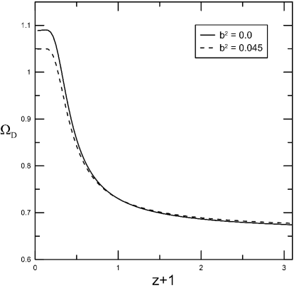
Figure 1: Density parameter ($\Omega_{D}$) versus redshift.

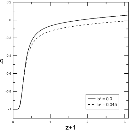
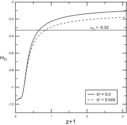
Figure 2: EoS and DP versus redshift.

In late time the logarithmic terms vanish and approximately we have $q\approx\frac{1+3\omega_{D}\Omega_{D}}{2}$. On the other hand, as is clear from figures 1 and 2, $\omega_{D}\rightarrow-1$ in this limit and so $q\approx\frac{1-3\Omega_{D}}{2}$. Now, let us to examine $\Omega_{D}$. For the late time $\Omega_{D}>1$, we have calculated approximately ($\Omega_{D}=1.08$), then for DP we must have ($q=-1.31$) which the phantom realm is successfully recovered. For all values $\Omega_{D}>1/3$, we have an accelerating expansion. Therefore, one can infer that in the matter dominated universe (early times) the expansion is decelerated and for DE dominated universe (late times) we have accelerated expansion.

4 Coincidence problem

In this section we will deal with the cosmic coincidence problem [11], in the framework of the presented model. Following the formalism proposed in [12] we determine the coupling value between dark energy and dark matter. Let us define

$$\zeta_{HDE}=1+\omega=\frac{\rho_{HDE}+p_{HDE}}{\rho_{HDE}},$$ (20)

$$\zeta_{m}=\frac{\rho_{m}+p_{m}}{\rho_{m}},$$ (21)

where $\zeta_{m}=1$ when $p_{m}=0$. To find how the density ratio $r=\rho_{m}/\rho_{D}$ evolves with redshift, we have

$$\dot{r}=\frac{dr}{dt}=\frac{\rho_{m}}{\rho_{HDE}}\Big{[}\frac{\dot{\rho}_{m}}{\rho_{m}}-\frac{\dot{\rho}_{HDE}}{\rho_{HDE}}\Big{]}.$$ (22)

With the use of (8) and (9) we have

$$\dot{r}=r\Big{[}\frac{Q}{\rho_{m}}+\frac{Q}{\rho_{NHDE}}+3H(\zeta_{HDE}-1)\Big{]},$$ (23)

which with $Q=3b^{2}(\rho_{m}+\rho_{D})$, takes the form

$$\dot{r}=3H[r(\zeta_{HDE}-1)+(1+r)^{2}b^{2}].$$ (24)

Thus, the equation $\dot{r}=0$ has the solutions

$$r_{\pm}=\frac{1-\zeta_{HDE}}{2b^{2}}-1\pm\Big{[}\Big{(}\frac{1-\zeta_{HDE}}{2b^{2}}-1\Big{)}^{2}-1\Big{]}^{\frac{1}{2}}.$$ (25)

Since the negative $b^{2}$s violate the second law of thermodynamics [13], we assume $b^{2}>0$. Indeed, observational constraints on the coupling constant have shown that the coupling parameter is a small positive value[14]. Under this condition the expression in the above square root will be positive if $\zeta\leq 1-4b^{2}$ or $\zeta\geq 1$. To address the cosmic coincidence problem [15], we rewrite the density ration as

$$r=-1+\frac{1}{\Omega_{D}}+\frac{2\beta a}{\Omega_{D}(\alpha+\beta a)\ln(\alpha+\beta a)}-\frac{2}{3}\frac{\beta^{2}a^{2}\omega}{\Omega_{D}(\alpha+\beta a)^{2}(\ln(\alpha+\beta a))^{2}},$$ (26)

in which we have used the relations (3), (6), (7) and (12). This equation shows $r$ depends on the scale factor, which in turn is a function of time. By ignoring the last two terms in the early times of cosmic evolution this equation reduces to $r=-1+\frac{1}{\Omega_{D}}$. However, as is shown in [16] the rate of time variation of $r$ is very slow compared to the scale factor. Therefore, with a good approximation we may write

$$r_{0}\approx-1+\frac{1}{\Omega_{D}},$$ (27)

where by $0$ we mean the value at the present time. Since according to the observational data [17], the value of the parameter $c$ is restricted: $0.5<c<1$ , the value of $\Omega_{D}$ varies in the interval $[0,1]$ and so we have $r_{0}\sim\mathcal{O}(1)$, see figure 3. This analysis shows that although the value of the parameter $c$ is important when one is going to determine the time varying form of the value of $r$, it does not play a major role in resolving the cosmic coincidence problem. The fact that $r_{0}\sim\mathcal{O}(1)$ in the early and late times shows that the cosmic coincidence is no longer seems to be a problem in this model.

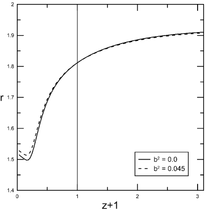
Figure 3: Variation of $r$ in terms of the redshift.

5 Statefinder diagnosis pair

Despite that the cosmic evolution is defined by the Hubble parameter as the rate of expansion and by the deceleration parameter accelerated or decelerated expansion is determined, these two parameters cannot clearly distinguish diverse models of DE. So, the progression in cosmological data during the last decade leads us to go beyond these two parameters. In order to perform more exact calculation concerning this issue a new diagnostic pair for dark energy has been proposed [18]. This pair $(r,s)$ which is called Statefinder is a geometrical diagnostic and allows us to characterize the properties of dark energy. Its definition is as follows

$$r=\frac{\dddot{a}}{aH^{3}}=1+\frac{\ddot{H}}{H^{3}}+3\frac{\dot{H}}{H^{2}},\hskip 14.22636pts=\frac{r-1}{3(q-\frac{1}{2})}.$$ (28)

To evaluate this pair in our model, all we need is to compute $\frac{\ddot{H}}{H^{3}}$ which may be obtained by taking a derivative of the relation (13). The result is

$$\begin{split}\frac{\ddot{H}}{H^{3}}=\frac{1}{1-\frac{\beta^{2}a^{2}}{(\alpha+\beta a)^{2}\ln(\alpha+\beta a)^{2}}+\frac{2\beta a}{(\alpha+\beta a)\ln(\alpha+\beta a)}-\frac{1}{2}(c^{2}+\Omega_{D})}\Big{(}\frac{\Omega^{\prime}_{D}\beta a}{(\alpha+\beta a)\ln(\alpha+\beta a)}~{}~{}~{}~{}~{}~{}~{}~{}~{}~{}~{}~{}~{}~{}~{}~{}\\ ~{}~{}~{}~{}+\frac{3\beta^{4}a^{4}}{(\alpha+\beta a)^{4}\ln(\alpha+\beta a)^{2}}(3+\frac{2}{\ln(\alpha+\beta a)})+\frac{\beta^{2}a^{2}}{(\alpha+\beta a)^{2}\ln(\alpha+\beta a)}(4-\Omega_{D})~{}~{}~{}~{}~{}~{}~{}~{}~{}~{}~{}~{}~{}~{}\\ ~{}-\frac{2\beta^{3}a^{3}}{(\alpha+\beta a)^{3}\ln(\alpha+\beta a)}(1+\frac{2}{\ln(\alpha+\beta a)})-\frac{2\beta a}{(\alpha+\beta a)\ln(\alpha+\beta a)}(\Omega_{D}-2)~{}~{}~{}~{}~{}~{}~{}~{}~{}~{}~{}~{}~{}~{}~{}~{}~{}\\ ~{}~{}~{}+\frac{\beta^{2}a^{2}}{(\alpha+\beta a)^{2}\ln(\alpha+\beta a)^{2}}(2-\Omega_{D})+\frac{3}{2}(b^{2}+1)\Omega^{\prime}_{D}-\big{(}\frac{\Omega_{D}\beta a}{(\alpha+\beta a)\ln(\alpha+\beta a)}(\Omega_{D}-2)~{}~{}~{}~{}~{}\\ ~{}~{}~{}+\frac{\beta^{2}a^{2}}{(\alpha+\beta a)^{2}\ln(\alpha+\beta a)}(1-\frac{\beta a}{(\alpha+\beta a)\ln(\alpha+\beta a)})+\frac{3}{2}((b^{2}+1)\Omega_{D}-1)\big{)}~{}~{}~{}~{}~{}~{}~{}~{}~{}~{}~{}~{}~{}~{}~{}~{}~{}~{}\\ ~{}~{}~{}\big{(}\frac{2\beta^{3}a^{3}}{(\alpha+\beta a)^{3}\ln(\alpha+\beta a)^{2}}(1+\frac{1}{\ln(\alpha+\beta a)})+\frac{2\beta a}{(\alpha+\beta a)\ln(\alpha+\beta a)}~{}~{}~{}~{}~{}~{}~{}~{}~{}~{}~{}~{}~{}~{}~{}~{}~{}~{}~{}~{}~{}~{}~{}~{}~{}~{}~{}~{}~{}\\ ~{}~{}~{}~{}-\frac{\beta^{2}a^{2}}{(\alpha+\beta a)^{2}\ln(\alpha+\beta a)}(2+\frac{4}{\ln(\alpha+\beta a)})-\frac{1}{2}\Omega^{\prime}_{D}\big{)}\Big{)}+(\frac{\dot{H}}{H^{2}})^{2}.~{}~{}~{}~{}~{}~{}~{}~{}~{}~{}~{}~{}~{}~{}~{}~{}~{}~{}~{}~{}~{}~{}~{}~{}~{}~{}~{}~{}~{}~{}~{}~{}~{}\end{split}$$ (29)

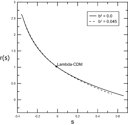
Figure 4: Statefinder pair.

With the help of this relation, we have plotted the statefinder pair ($r$ in terms of $s$) in figure 4. It is seen from this figure that as the universe expands, by increasing the parameter $r$ the parameter $s$ decreases (from positive to negative values). The point $(r,s)=(1,0)$ corresponds to the $\Lambda$CDM model. The state finder trajectory indicates the Chaplygin gas behavior (where $s<0,r>1$) and the phantom like behavior (where $s>0,r<1$).

6 Om-Diagnostic

In order to study and differentiating different stages of the universe, the Om-diagnostic tool has been proposed [20]. Using this tool and according to resulted curves in the final plot, one can distinguish the behavior of DE model and divide it into two sections. Phantom-like ($\omega_{D}<-1$) behavior corresponds to the positive values in the Om(x) trajectories and quintessence ($\omega_{D}>-1$) comes from its negative value. The Om-diagnostic tool can be explained as

$$\mbox{Om}(x)=\frac{h(x)^{2}-1}{x^{3}-1},$$ (30)

where $h(x)=H(x)/H_{0}$ and $x=ln(z+1)^{-1}$. The evolution of Om-diagnostic tool in terms of the redshift is plotted in figure 5. It can be seen that for both non-interacting and interacting models the trajectories present negative values which show the quintessence behavior of the universe. Also, it is clear that in the late time ($z<0$) the positive value of trajectories implies phantom behavior which indicates uniformity with the equation of state parameter as seen in figure 2.

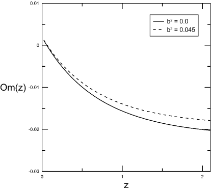
Figure 5: The Om-diagnostic tool versus $z$.

7 Data analysis methods

In this section, we fit present model using the recent observational data sets including SN Ia, BAO and CMB. We have used the minimized chi-square test and obtain the best fit values of the free parameters for $1\sigma$ and $2\sigma$ confidence region.
For the SN Ia data sets, we use the cJLA data set of 31 check points (30 bins) with the range of redshift $0.01<z<1.3$ [21]. The corresponding $\chi^{2}$ function is

$$\chi^{2}_{SNIa}=r^{t}C^{-1}_{b}r,$$ (31)

in which

$$r=\mu_{b}-M-5log_{10}d_{L},$$ (32)

where where $\mu_{b}$ is the observational distance modulus, $M$ is a free normalization parameter and $C_{b}$ is the covariance matrix of $\mu_{b}$, see Table F.2 in [21]. Also, the dimensionless luminosity distance is defined as

$$d_{L}=\frac{c(1+z)}{H_{0}}\int_{0}^{z^{\prime}}\frac{dz^{\prime}}{[(1+z^{\prime})^{2}(1+\Omega_{m}z^{\prime})-z^{\prime}(2+z^{\prime})\Omega_{D}]^{0.5}}.$$ (33)

For BAO we use data of BOSS DR12 including six BAO data points [22]. The $\chi^{2}_{BAO}$ function is defined as

$$\chi^{2}_{BAO}=X^{t}C_{BAO}^{-1}X,$$ (34)

which for $X$ we can write

$$X=\left(\begin{array}[]{c}\frac{D_{M}(0.38)r_{s,fid}}{r_{s}(z_{d})}-1512.39\\ \frac{H(0.38)r_{s}(z_{d})}{r_{s}(z_{d})}-81.208\\ \frac{D_{M}(0.51)r_{s,fid}}{r_{s}(z_{d})}-1975.22\\ \frac{H(0.51)r_{s}(z_{d})}{r_{s}(z_{d})}-90.9\\ \frac{D_{M}(0.61)r_{s,fid}}{r_{s}(z_{d})}-2306.68\\ \frac{H(0.51)r_{s}(z_{d})}{r_{s}(z_{d})}-98.964\end{array}\right),$$ (35)

where $r_{s,fid}=$147.78 Mpc is the sound horizon of fiducial model, $D_{M}(z)=(1+z)D_{A}(z)$ is the comoving angular diameter distance. The sound horizon at drag epoch $r_{s}(z_{d})$ may be expressed as

$$r_{s}(z_{d})=\int_{z_{d}}^{\infty}\frac{c_{s}(z)}{H(z)}dz,$$ (36)

where $c_{s}=1/\sqrt{3(1+R_{b}/(1+z))}$ is the sound speed with $R_{b}=31500\Omega_{b}h^{2}(2.726/2.7)^{-4}$. The covariance matrix can be downloaded from the online files of [22]:

$$C^{-1}_{BAO}=\begin{pmatrix}624.707&23.729&325.332&8.34963&157.386&3.57778\\ 23.729&5.60873&11.6429&2.33996&6.39263&0.968056\\ 325.332&11.6429&905.777&29.3392&515.271&14.1013\\ 8.34963&2.33996&29.3392&5.42327&16.1422&2.85334\\ 157.386&6.39263&515.271&16.1422&1375.12&40.4327\\ 3.57778&0.968056&14.1013&2.85334&40.4327&6.25936\end{pmatrix}.$$ (37)

Probing the whole expansion history until the last scattering phase, we use Planck 2015 for CMB [23]. The $\chi^{2}_{CMB}$ function is

$$\chi^{2}_{CMB}=q_{i}-q^{data}_{i}Cov^{-1}_{CMB}(q_{i},q_{j}),$$ (38)

where $q_{1}=R(z_{*})$, $q_{2}=l_{a}(z_{*})$ and $q_{3}=\omega_{b}$. $Cov_{CMB}$ is the covariance matrix [23]. The data of Planck 2015 are

$$q^{data}_{1}=1.7382,\hskip 14.22636ptq^{data}_{2}=301.63,\hskip 14.22636ptq^{data}_{3}=0.02262.$$ (39)

The acoustic scale $l_{A}$ can be defined as

$$l_{A}=\frac{3.14d_{L}(z_{*})}{(1+z)r_{s}(z_{*})},$$ (40)

where $r_{s}(z_{*})$ is the comoving sound horizon at the decoupling time ($z_{*}$). The redshift of the decoupling time is [24]

$$z_{*}=1048\left[1+0.00124(\Omega_{b}h^{2})^{-0.738}\right]\left[1+g_{1}(\Omega_{m}h^{2})^{g_{2}}\right],$$ (41)

where

$$g_{1}=\frac{0.0783(\Omega_{b}h^{2})^{-0.238}}{1+39.5(\Omega_{b}h^{2})^{-0.763}},~{}~{}~{}g_{2}=\frac{0.560}{1+21.1(\Omega_{b}h^{2})^{1.81}}.$$ (42)

The CMB shift parameter is [25]

$$R=\sqrt{\Omega_{m_{0}}}\frac{H_{0}}{c}r_{s}(z_{*}).$$ (43)

Finally, the total $\chi^{2}$ is

$$\chi^{2}_{total}=\chi^{2}_{SNIa}+\chi^{2}_{BAO}+\chi^{2}_{CMB}.$$ (44)

By minimizing the above quantity we can perform the best-fit values of the free parameters. Considering the $1\sigma$ and $2\sigma$confidence level, the best-fit values of $\alpha$, $\beta$, $c$ and $\Omega_{m0}$ are shown in table 1.

Parameters	cJLA + BOSS DR12 + Planck2015
$\Omega_{m}$	$0.268^{+0.008~{}+0.010}_{-0.007~{}-0.009}$
$\alpha$	$3.361^{+0.332~{}+0.483}_{-0.401~{}-0.522}$
$\beta$	$5.560^{+0.541~{}+0.780}_{-0.510~{}-0.729}$
$c$	$0.777^{+0.023~{}+0.029}_{-0.017~{}-0.023}$
$b^{2}$	$0.045$
$M$	$10.7$

Table 1: 68.3% and 95.4% error marginalized result for each parameter.

By using of the latest observational data sets namely cJLA, Boss DR12 and Planck 2015, we have plotted 1D marginalized posterior distributions and 2D confidence region of the important parameters of the current model in figure 6.

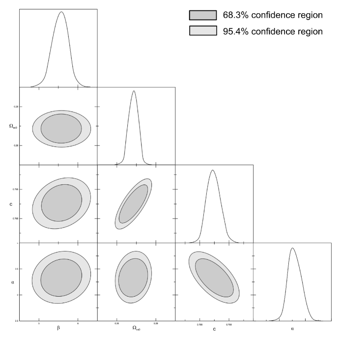
Figure 6: The 2D 68.3% and 95.4% confidence level for $\alpha$, $\beta$, $\Omega_{m0}$ and c.

8 Summary

In this paper we have applied a new HDE model (firstly proposed in [6] inspired by the DGP braneworld theory) to the BD gravity in both interacting ($b^{2}=0.045$-fitted with the recent observational data) and non-interacting ($b^{2}=0$) cases. The Hubble radius $L=H^{-1}$ plays the role of the system’s IR cutoff. Following [5], we have taken a logarithmic BD scalar field which gives a dynamical DP. Then we evaluated and plotted the density parameter, EoS and DP in terms of redshift. We found that in both interacting and non-interacting levels, the corresponding universe is expanding with accelerating rate. Our numerical results shows that the acceleration of accelerated expansion of the universe increases exponentially after $z=0.75$. The DP for both interacting and non-interacting models resulted an universe with accelerating expansion and undergoes from matter to DE dominated universe approximately at $z\approx 0.55$ which is consistent with recent observational data $0.4<z<1$ [19] and mimics the phantom dark energy at the late time. We also performed the statefinder diagnosis pair tool with different value of $c$ parameter which leads to different trajectories in $s-r$ plane. Since the $\Lambda$CDM is the main standard model of dark energy, hence we have tried to measure the deviation of the points in $s-r$ plane from the point $(r,s)=(1,0)$ correspond to the $\Lambda$CDM. Using the state finder pair tool indicated a behavior similar to Chaplygin gas ($s<0,r>1$).
In the language of the Om-diagnostic tool, its variation in terms of the redshift by taking $x=ln(1+z)^{-1}$, shows negative values which implies the quintessence behavior. Finally, in order to check compatibility with observational data and fitting the free parameters, we used cJLA compilation for SNIa, six observational points of BAO from BOSS DR12 and Planck 2015 for CMB. This combination of the resent observational data sets results in $\Omega_{m}=0.268^{+0.008~{}+0.010}_{-0.007~{}-0.009}$, $\alpha=3.361^{+0.332~{}+0.483}_{-0.401~{}-0.522}$, $\beta=5.560^{+0.541~{}+0.780}_{-0.510~{}-0.729}$, $c=0.777^{+0.023~{}+0.029}_{-0.017~{}-0.023}$ and $b^{2}=0.045$ with $1\sigma$ and $2\sigma$ confidence interval.
Acknowledgement
We would like to thank the referee for insightful comments which improved the quality of the paper. This work has been supported financially by Research council of the Central Tehran Branch, Islamic Azad University.

References

-
[1]
K. Bamba, S. Capozziello, S. Nojiri and S. D. Odintsov,
Astrophys. Space Science 342 (2012) 155 (arXiv:
1205.3421 [gr-qc])
S. Tsujikawa, Dark energy: investigation and modeling (arXiv: 1004.1493 [astro-ph.CO])
M. Li, X.-D. Li, S. Wang and Y. Wang, Commun. Theor. Phys. 56 (2011) 525 (arXiv: 1103.5870 [astro-ph.CO])
B. Wang, E. Abdalla, F. Atrio-Barandela and D. Pavon, Dark Matter and Dark Energy Interactions: Theoretical Challenges, Cosmological Implications and Observational Signatures (arXiv: 1603.08299 [astro-ph.CO]) -
[2]
S. Wang, Y. Wang and M. Li, Holographic Dark Energy
(arXiv: 1612.00345 [astro-ph.CO])
B. Wang, Y. Gong and E. Abdalla, Phys. Lett. B 624 (2005) 141 (arXiv: hep-th/0506069)
M. Li, X.-D. Li, S. Wang, Y. Wang and X. Zhang, JCAP 0912 (2009) 014 (arXiv: 0910.3855 [astro-ph.CO])
M Ito, Europhys. Lett. 71 (2005) 712 (arXiv: hep-th/0405281)
H. Wei and S. N. Zhang, Phys. Rev. D 76 (2007) 063003 (arXiv: 0707.2129 [astro-ph]) -
[3]
G. ’tHooft, Dimensional Reduction in Quantum Gravity (arXiv: gr-qc/9310026)
L. Susskind, J. Math. Phys. 36 (1995) 6377
A. Cohen, D. Kaplan and A. Nelson, Phys. Rev. Lett. 82 (1999) 4971 -
[4]
M. Li, Phys. Lett. B 603 (2004) 1
Q. G. Huang and M. Li, JCAP 0408 (2004) 013 - [5] P. Kumar and C.P. Singh, Astrophys. Space Sci. 362 (2017) 52 (arXiv: 1609.02751 [gr-qc])
- [6] A. Sheykhi, M. H. Dehghani and S. Ghaffari, Int. J. Mod. Phys. D 25 (2016) 1650018 (arXiv: 1506.02505 [gr-qc])
- [7] K. Nozari, N. Behrouz and A. Sheykhi, Int. J. Theor. Phys. 52 (2013) 2351
- [8] C. Deffayet, Phys. Lett. B 502 (2001) 199
- [9] S. D. H. Hsu, Phys. Lett. B 594 (2004) 13 (arXiv: hep-th/0403052)
-
[10]
L. Amendola, Phys. Rev. D 62 (2000) 043511 (arXiv: astro-ph/9908023)
L. Amendola, Phys. Rev. D 60 (1999) 043501 (arXiv: astro-ph/9904120)
B. Wang, Y. Gong and E. Abdalla, Phys. Lett. B 624 (2005) 141
G. Caldera-Cabral, R. Maartens and L. A. Ureoa-Lopez, Phys. Rev. D 79 (2009) 063518
Z.-K. Guo, N. Ohta, and S. Tsujikawa, Phys. Rev. D 76 (2007) 023508
G. Huey and B. D. Wandelt, Phys. Rev. D 74 (2006) 023519 (arXiv: astro-ph/0407196) - [11] D. Pavon and W. Zimdah, Phys. Lett. B 628 (2005) 206 (arXiv: gr-qc/0505020)
- [12] Z.-K. Guo and Y.-Z. Zhang, Phys. Rev. D 71 (2005) 023501
- [13] D. Pavon and B. Wang, Gen. Rel. Grav. 41 (2009) 1 (arXiv: 0712.0565 [gr-qc])
- [14] C. Feng, B. Wang, E. Abdalla and R.-K. Su, Phys. Lett. B 665 (2008) 111 (arXiv: 0804.0110 [astro-ph])
-
[15]
D. Pavon and W. Zimdahl, Phys. Lett. B 628 (2005)
206 (arXiv: gr-qc/0505020)
N. Banerjee and D. Pavon, Phys. Lett. B 647 (2007) 477 (arXiv: gr-qc/0702110)
H. Zhang, H. Yu, Z.-H. Zhu and Y. Gong, Phys. Lett. B 678 (2009) 331 - [16] S. del Campo, R. Herrera and D. Pavon, Phys. Rev. D 78 (2008) 021302 (arXiv: 0806.2116 [astro-ph])
-
[17]
M. Li, X.-D. Li, Y.-Z. Ma, X. Zhang and Z. Zhang, JCAP 09 (2013)
021 (arXiv: 1305.530 [astro-ph.CO])
L. Xu, Phys. Rev. D. 87 (2013) 043525 (arXiv: 1302.2291 [astro-ph.CO]) -
[18]
V. Sahni, T. D. Saini, A. A. Starobinsky and U. Alam,
JETP Lett. 77 (2003) 201 (arXiv: astro-ph/0201498)
U. Alam, V. Sahni, T. D. Saini and A. A. Starobinsky, Mon. Not. Roy. Astron. Soc. 344 (2003) 1057 (arXiv: astro-ph/0303009) - [19] V. Salvatelli, A. Marchini, L. Lopez-Honorez and O. Mena, Phys. Rev. D 88 (2013) 023531 (arXiv: 1304.7119 [astro-ph.CO])
- [20] V. Sahni, A. Shafieloo and A. A. Starobinsky, Phys. Rev. D 78 (2008) 103502 (arXiv: 0807.3548 [astro-ph])
- [21] M. Betoule, et al. Astron. Astrophys. 568 (2014) A22 (arXiv: 1401.4064 [astro-ph.CO])
- [22] S. Alam, et al. MNRS 2617-2652 (2017) 470
- [23] P. A. R. Ade, et al. Astron. Astrophys. 594 (2016) A13
- [24] W. Hu and N. Sugiyama, Astrophys. J. 471 (1996) 542
- [25] Y. Wang and P. Mukherjee, Phys. Rev. D 76 (2007) 103533 (arXiv: astro-ph/0703780)