Maximum-Likelihood Power-Distortion Monitoring for GNSS Signal Authentication
Abstract
We propose an extension to the so-called PD detector. The PD detector jointly monitors received power and correlation profile distortion to detect the presence of GNSS carry-off-type spoofing, jamming, or multipath. We show that classification performance can be significantly improved by replacing the PD detector’s symmetric-difference-based distortion measurement with one based on the post-fit residuals of the maximum-likelihood estimate of a single-signal correlation function model. We call the improved technique the PD-ML detector. In direct comparison with the PD detector, the PD-ML detector exhibits improved classification accuracy when tested against an extensive library of recorded field data. In particular, it is (1) significantly more accurate at distinguishing a spoofing attack from a jamming attack, (2) better at distinguishing multipath-afflicted data from interference-free data, and (3) less likely to issue a false alarm by classifying multipath as spoofing. The PD-ML detector achieves this improved performance at the expense of additional computational complexity.
Index Terms:
satellite navigation systems, Global Positioning System, navigation security, GNSS spoofing, GNSS jamming, GNSS authenticationI Introduction
Civil GNSS receivers are susceptible to counterfeit spoofing signals [1, 2, 3, 4]. To defend against spoofing attacks, several algorithms have been developed and reported in the literature. A comprehensive review of GNSS spoofing detection methods is provided in [5], where methods are broadly categorized as (1) cryptographic techniques, (2) geometric techniques that exploit angle-of-arrival diversity, or (3) signal processing techniques that do not fall into categories (1) or (2), such as the PD detector [6].
Within the latter category, the subset of techniques which do not require additional hardware and can be implemented via a firmware update are particularly attractive for widespread adoption. Of these, the PD detector, which jointly monitors received power and correlation profile distortion, has been shown to reliably alarm in the presence of carry-off-type spoofing or jamming attacks while maintaining a low multi-channel false alarm rate, when tested against 27 high quality data recordings [6].
An appealing attribute of the PD detector is simplicity: its received power and correlation profile distortion measurements are computationally lightweight and amenable to analysis. However, when tested in [6] against an extensive set of empirical data, the PD detector was shown to incorrectly classify most instances of spoofing as jamming, and its % single-channel false alarm rate (false declaration of interference-free or multipath-afflicted signals as spoofing or jamming), is too high for some applications of practical interest. This correspondence article extends the PD detector to address these shortcomings, and for compactness, it is intended to be read alongside the original PD detector paper [6].
The PD detector’s shortcomings stem from two undesirable features of the symmetric difference (SD) as a measure of distortion. First, the standard SD involves only a pair of complex correlation function taps and is not particularly sensitive to correlation function distortion not aligned with these taps. Thus, if the SD taps are closely spaced around the prompt correlation tap, then the SD can be a good distortion measure during the initial stage of a carry-off-type spoofing attack, but quickly becomes insensitive as the attack proceeds. Second, the SD depends on the receiver’s code tracking loop to align its pair of taps symmetrically about the authentic correlation peak. But even in the absence of spoofing or significant multipath, thermal noise prevents the code tracking loop from achieving perfectly symmetric alignment. As a consequence, the SD tends to exaggerate the actual distortion under the null (thermal noise only) and jamming hypotheses.
The PD-ML detector’s distortion measure avoids both of these limitations. It begins by measuring the correlation function at many more than two taps, which offers two advantages: (1) the PD-ML detector can be made sensitive to distortion far from the prompt tap, thus extending the range of spoofing-to-authentic code offsets over which it can detect spoofing, and (2) the PD-ML detector’s measure of distortion can be made independent of the receiver’s code and carrier tracking loops in the sense that small tracking errors in no way affect the reported distortion. This is done by exploiting data from the additional taps to obtain the maximum-likelihood estimates of the amplitude, code phase, and carrier phase of the correlation peak in a single-signal correlation function model. After removing this estimated correlation function model from each of the correlation taps, the PD-ML detector takes as its distortion measure the squared magnitude of the normalized post-fit residuals. As will be shown, distortion measured in this way permits more accurate classification of jamming, multipath, and spoofing than distortion based on a simple symmetric difference.
Herein, we adopt, without alteration, several aspects of the PD detector [6]. In particular, the signal models (Section II of [6]), probability distributions (Section III of [6]), and the Monte-Carlo-type Bayes-optimal decision rule design strategy developed (Section VI of [6]). This correspondence, a significant extension of our conference paper [7], exploits multi-tap maximum-likelihood multipath estimation and demonstrates the proposed PD-ML detector’s advantages through a direct comparison with the original PD detector on the same experimental data recordings and using the same Bayes-optimal detector design strategy as presented in [6]. Details of the PD-ML detector are presented in Section III, followed by simulated (Section IV) and experimental (Section VI) evaluation of its classification performance. All source code required to generate decision rules using the PD-ML detector is publicly available at https://github.com/navSecurity/P-D-defense.
II Signal Models
For a thorough discussion of the GNSS signal models adopted in this work, starting with the pre–correlation signal model, the reader is directed to the paper on the PD detector [6]. However, to provide the context necessary to understand this paper’s proposed extension to the PD detector, a brief review of the single-interferer post-correlation model assumed in [6], which is adapted from [8], is presented here. This model gives the complex-valued receiver correlation function at some arbitrary code offset, or lag, , as
| (1) |
where is the average value of the automatic gain control scaling factor over the th accumulation interval, and , , are the complex correlation function components corresponding to the authentic signal, the interference signal, and thermal noise, respectively.
Just as in [6], the correlation components for the authentic and interference signal, and , are assumed to be modeled as
where is the GNSS auto-correlation function, and, at the th accumulation interval, is the average value of the authentic signal’s power, is the average interference signal’s power advantage over the authentic signal (i.e., ), and is the average value of the code offset , with being the true code phase of the authentic signal and being the receiver’s estimate of the same. Similar definitions follow for , , and [6].
The thermal noise component of the correlation function, , is modeled as having independent in-phase (real) and quadrature (imaginary) components, each modeled as a zero-mean Gaussian white discrete-time process:
As discussed in [9], thermal noise is correlated in the lag domain. For samples within of each other, where is the chip-width of the GNSS signal, correlation in is modeled as
Here, ∗ denotes the complex conjugate and is the variance of the in-phase and quadrature components of , which is related to the spectral density of a white noise process that is modeled as the sum of two independent components associated with thermal noise and multi-access noise. The spectral density of the thermal noise, , is assumed to be constant whereas the spectral density of the multi-access noise, , is assumed to be variable, as detailed in [6]. When averaging over an accumulation interval the variance is given as .
III Measurement Models
Like the PD detector, the PD-ML detector simultaneously monitors received power and correlation function distortion. Its received power monitor is identical to the PD detector’s, as described in [6], but its distortion monitor differs considerably. This section develops the measurement model for the PD-ML detector’s distortion monitor.
The PD-ML detector models the in-phase and quadrature (IQ) samples of the correlation function as a function of only the authentic signal and thermal noise, neglecting in (1). It employs a maximum-likelihood estimator to estimate the authentic signal’s amplitude, code phase, and carrier phase, and takes the squared magnitude of the normalized post-fit residuals as its measure of correlation profile distortion.
Maximum-likelihood estimation based on GNSS correlation data is well-established in the literature [10, 11, 12, 13, 14]. It is routinely employed within high-end GNSS receivers for multipath mitigation. This paper’s distortion monitor adapts the particular maximum-likelihood estimator developed in [14], as described subsequently, though other approaches could be adopted in the PD-ML detector in a straight-forward manner.
III-A Multi–Tap Maximum–Likelihood Correlation Function Estimator
Let be the number of signal taps devoted to maximum-likelihood estimation. For convenience, we assume that is odd and that taps are distributed, so the centermost tap is approximately aligned with the receiver’s estimated correlation function peak and the remaining taps are spaced evenly across the range . The uniform tap interval is
and the vector of tap locations is given by
with representing the th tap location, .
Modeling the correlation function as interference-free (i.e., for all ), the complex-valued th tap at time index is expressed in terms of the authentic signal’s gain-controlled amplitude , carrier phase , and code phase as
| (2) |
The parameters are estimated according to this model by an adaptation of the maximum likelihood technique in [14]. This approach separates estimation of the code phase from estimation of amplitude and carrier phase by exploiting the linear relationship
| (3) |
where and the observation matrix is
| (4) |
First, a coarse search is performed by setting the code phase estimate for and, for each candidate , solving for the maximum-likelihood estimate of :
| (5) |
where is the Toeplitz matrix that accounts for the correlation of the complex Gaussian thermal noise among the taps [14]. The th element of is , where is the tap spacing.
The cost corresponding to each set of estimates , is calculated as
| (6) |
where the norm is defined such that . The two sets of estimates yielding the smallest cost are extracted. Because the cost is proportional to the negative log likelihood function, the set with the minimum cost is the maximum likelihood estimate.
In a second step, a refined code phase estimate is obtained by a bisecting search between the two lowest-cost code phase estimates. At each bisection point, new amplitude and carrier phase estimates are determined by re-evaluating (5). The process is repeated until is no longer significantly reduced. Upon convergence, the resulting estimates are accepted as the maximum-likelihood estimates , and the corresponding is taken as the distortion measurement . A small indicates that the single-signal model (III-A) accurately fits the correlation function data at time ; a large indicates the opposite, suggesting that multipath or spoofing interference is present. This is illustrated in Fig. 1, where the top panel illustrated a nominal scenario and the bottom panel represents a spoofing scenario.
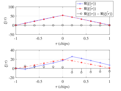
This distortion metric is more informative than the symmetric difference metric used in [6] because it (1) exploits data from taps, whereas the symmetric difference only uses two, and (2) is insensitive to noise- or dynamics-induced misalignment of the prompt tap (located at ) with the authentic signal peak, whereas the symmetric difference falsely reports distortion in this circumstance.
IV Decision Rule
Design of the PD-ML’s decision rule follows the same procedure outlined in the PD detector [6], but with the new distortion metric replacing the symmetric difference. First, we simulate the post-correlation model (1) using the same model priors, parameter probability distributions, and probability transition mechanisms for each hypothesis as in [6]. The hypotheses are denoted for , where the null hypothesis corresponds to the interference-free case, and correspond respectively to multipath, spoofing, and jamming. For each Monte-Carlo sample under each hypothesis, a power measurement is made as in [6] and a distortion measurement is made as described above.
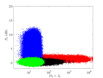
Fig. 2. shows the power-distortion measurements from a Monte-Carlo simulation with taps. One can observe the following behavior of the new distortion metric :
-
•
Under (interference-free): is small, as only thermal noise is present.
-
•
Under (multipath-afflicted): is similar to that of the case when multipath is weak but attains a significant magnitude as multipath severity increases.
-
•
Under (spoofing): overlaps with that of multipath (), but exhibits a much wider range.
-
•
Under (jamming): is nearly indistinguishable from distortion under , as jamming has little effect on the gain-controlled correlation function.
Based on the simulated data shown in Fig. 2, decision regions corresponding to a Bayes-optimal decision rule for a parameter-dependent cost were found as described in [6]. Fig. 3 shows the optimum decision regions for .
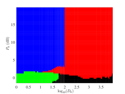
Figs. 2 and 3 are analogous to Figs. 6 and 7 within [6]. When comparing these figures for PD and PD-ML, the most notable difference being that the PD-ML’s distortion metric extends over a much larger domain than the PD detector (i.e., notice the logarithmic scale in Figs. 2 and 3). This increased distortion sensitivity could potentially lead to better discrimination between jamming and spoofing and, likewise, between interference free and multipath-afflicted.
Table I shows classification statistics as evaluated by applying the Bayes-optimal rule to a validation set of Monte-Carlo-generated measurements that used the same assumptions as the distributions shown in Fig. 2. This table reveals that the PD-ML detector exhibits similar theoretical performance to the PD detector. Both tend to misclassify multipath () as interference free () because of the low cost assigned to this error when multipath is mild. Otherwise, the PD-ML detector, like the PD detector, exhibits high detection power and a low false alarm rate.
| Decision | True Scenario | |||
|---|---|---|---|---|
| 0.9947 | 0.9083 | 0.0670 | 0.0039 | |
| 0 | 0.0698 | 0.0117 | 0 | |
| 0.0043 | 0.0214 | 0.8463 | 0.0155 | |
| 0.0010 | 0.0005 | 0.0750 | 0.9806 | |
The sensitivity of the PD-ML detector’s performance to the number of taps was explored. Starting from taps, the entire design process was repeated for several choices of of decreasing value. Performance generally decreased with reduced . It was found that at least taps were needed to maintain a level of theoretical detector performance comparable with that of the PD detector (Table I of [6]).
V Experimental Data
An independent evaluation of PD-ML was carried out against 27 empirical GNSS data recordings, including 6 recordings of various spoofing scenarios [15], 14 multipath-dense scenarios, 4 jamming scenarios of different power levels, and 3 scenarios exhibiting negligible interference beyond thermal and multi-access noise. The details of the data sets, including their source, are given Table II of [6]. To ensure a fair and direct comparison with the PD detector, these data were pre-processed using the same approach as in [6].
VI Experimental Results
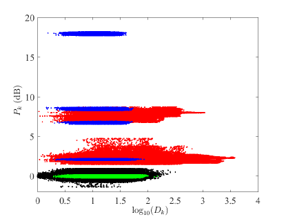
This section presents the experimental performance assessment of the PD-ML detector based on the decision regions shown in Fig. 3 being applied to the observations, shown in Fig. 4, derived from the 27 experimental data recordings. Table II summarizes the PD-ML detector’s overall performance against the experimental data in terms of classification statistics.
| Decision | True Scenario | |||
| 0.8500 | 0.4337 | 0.0001 | 0 | |
| 0.1500 | 0.5632 | 0 | 0 | |
| 0 | 0.0031 | 0.8289 | 0.2176 | |
| 0 | 0 | 0.1676 | 0.7824 | |
When comparing this table to the corresponding one for the PD detector (Table III in [6]), the important result is that classification performance accuracy under a spoofing attack is improved more than four-fold. That is, with the PD detector, spoofing attacks were classified as jamming for 82% of experimental spoofing detection trials. This is reduced to only 17% with the PD-ML detector. All but 0.01% of spoofing or jamming attacks result in an alarm. Compared to the PD-ML detector, there is nearly a two-fold decrease in spoofing false alarms under (multipath). Finally, the PD-ML detector correctly classifies of the multipath data, compared to only 12% with the PD detector.
Thus, although the PD-ML detector does not enjoy any significant advantage over the PD detector when tested against Monte-Carlo-simulated data (Table I), it significantly outperforms the PD detector when tested against the empirical dataset. A likely explanation is that the PD-ML detector’s greater number of correlation taps (for Table II, ) allow spoofer-induced distortion to be readily detected over a wider range of spoofer-to-authentic code phase offset.
The PD-ML detector was also applied to the especially stealthy tb7 attack [16], which mounts a nulling attack during the beginning of the attack before pull-off. This attack would be extremely difficulty to realize outside the laboratory. Soon after pull-off begins, the PD-ML detector correctly classifies the attack as spoofing. Against the attack portion of the scenario, its decision rates were : 17%, : 17%, : 66%, and : 0%, as compared to : 14%, : 10%, : 70%, and : 6% for the PD detector. The PD-ML detector’s attack detection power is lower than the PD detector’s on this attack, but it never mis-attributes spoofing as jamming. This can be attributed to especially subtle nature of this attack. In particular, a larger portion of the period prior to pull-off is labeled as multipath by the PD-ML detector due to the authentic signal being nulled.
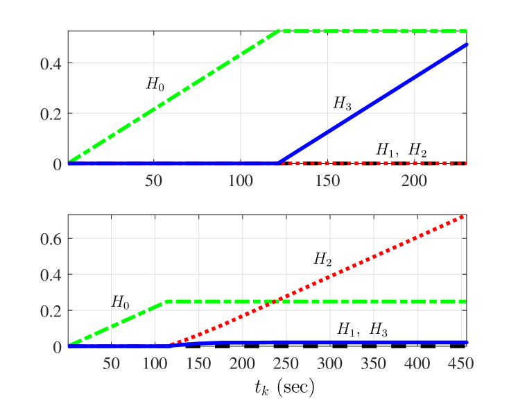
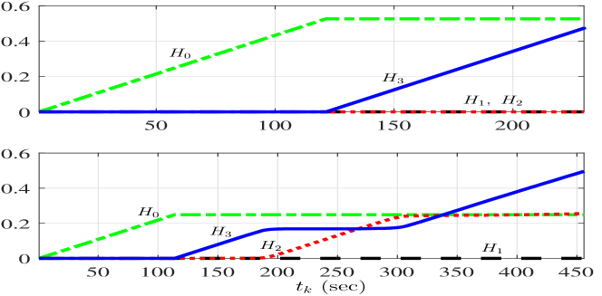
The PD-ML detector’s superior spoofing vs. jamming classification is further illustrated in of Fig. 5, which shows the single-channel cumulative time history of the detector’s decisions for example jamming and spoofing attack scenarios using both the proposed PD-ML detector and the original PD detector. Within Fig. 5, 5(b) shows the reproduced Fig. 10 from [6] and illustrates the performance of the PD detector. In Fig. 5(a), detection is assessed against the same attack scenarios using the proposed PD-ML detector. Like the PD detector, in the jamming scenario (top panels), the attack is detected immediately at its onset, and continuously declared thereafter. In the spoofing scenario (bottom panels), the attack is detected immediately, and briefly classified as jamming because the spoofer’s near-perfect initial code-phase alignment causes little distortion (and, indeed, little harm to the receiver). However, as the spoofer begins its pull-off, the PD-ML detector correctly declares the attack to be spoofing and does so for the remainder of the attack. This is different from the PD detector in Fig. 5(b) , which declares the attack as an almost equal blend of jamming and spoofing as the pull-off proceeds.
Finally, when comparing the PD-ML detector to the PD detector is it important to point out that the PD-ML detector’s distortion metric requires more computational complexity. In particular, the PD detector’s distortion metric simply subtracts two taps to determine symmetric difference [6]. In contrast, the PD-ML detector requires a Maximum-Likelihood estimation of the correlation function and requires access to multiple tap data. Further, this estimator is executed multiple times. First over a coarse search for the code-phase and then during a refinement stage via bisection. As such, one should consider complexity against performance when deciding to the chose the PD-ML detector or the PD detector.
VII Conclusions
This paper presented the PD-ML detector, an extension to the recently-proposed PD detector. The PD-ML detector employs a maximum-likelihood multipath estimator and uses the magnitude of its post-fit residuals to monitor distortion, as opposed to the PD detector’s use of a symmetric difference. Like the PD detector, the PD-ML detector traps a would-be attacker between simultaneous monitoring of received power and complex correlation function distortion. In a head-to-head evaluation based on 27 high-quality experimental recordings of attack and non-attack scenarios, the PD-ML detector was shown to be significantly better at classifying spoofing vs. jamming, exhibiting a nearly four-fold improvement. In addition, the PD-ML detector was shown to significantly improve the classification of multipath data. The improved performance improvement comes at the expense of the additional computational complexity associated with producing correlation products from a larger number of taps and processing these with a maximum-likelihood estimator. Thus, depending on the application, the simpler PD detector may be more favorable despite the better classification performance offered by the PD-ML detector. In future work, it will be important to evaluate the the sensitivity of both the PD-ML and PD detectors on receiver’s with a narrower front-end bandwidth (i.e., 2 MHz).
The code for the PD-ML detector has been made available at the same repository as the PD detector: https://github.com/navSecurity/P-D-defense [17].
Acknowledgements
Jason Gross’s work on this project was supported in part by a West Virginia University Big XII Faculty Fellowship. Todd Humphreys’s work on this project has been supported by the National Science Foundation under Grant No. 1454474 (CAREER) and by the Data-supported Transportation Operations and Planning Center (DSTOP), a Tier 1 USDOT University Transportation Center.
References
- [1] T. E. Humphreys, B. M. Ledvina, M. L. Psiaki, B. W. O’Hanlon, and P. M. Kintner, Jr., “Assessing the spoofing threat: Development of a portable GPS civilian spoofer,” in Proceedings of the ION GNSS Meeting. Savannah, GA: Institute of Navigation, 2008.
- [2] D. P. Shepard, T. E. Humphreys, and A. A. Fansler, “Evaluation of the vulnerability of phasor measurement units to GPS spoofing attacks,” International Journal of Critical Infrastructure Protection, vol. 5, no. 3-4, pp. 146–153, 2012.
- [3] A. J. Kerns, D. P. Shepard, J. A. Bhatti, and T. E. Humphreys, “Unmanned aircraft capture and control via GPS spoofing,” Journal of Field Robotics, vol. 31, no. 4, pp. 617–636, 2014.
- [4] J. Bhatti and T. Humphreys, “Hostile control of ships via false GPS signals: Demonstration and detection,” Navigation, Journal of the Institute of Navigation, vol. 64, no. 1, 2017.
- [5] M. L. Psiaki and T. E. Humphreys, “GNSS spoofing and detection,” Proceedings of the IEEE, vol. 104, no. 6, pp. 1258–1270, 2016.
- [6] K. D. Wesson, J. N. Gross, T. E. Humphreys, and B. L. Evans, “GNSS signal authentication via power and distortion monitoring,” IEEE Transactions on Aerospace and Electronic Systems, 2018, to be published; preprint available at https://arxiv.org/abs/1702.06554.
- [7] J. Gross and T. E. Humphreys, “GNSS spoofing, jamming, and multipath interference classification using a maximum-likelihood multi-tap multipath estimator,” Proceedings of the ION International Technical Meeting, Jan. 2017.
- [8] R. D. J. van Nee, “Spread-spectrum code and carrier synchronization errors caused by multipath and interference,” IEEE Transactions on Aerospace and Electronic Systems, vol. 29, no. 4, pp. 1359–1365, 1993.
- [9] A. J. Van Dierendonck, P. Fenton, and T. Ford, “Theory and performance of narrow correlator spacing in a GPS receiver,” Navigation, Journal of the Institute of Navigation, vol. 39, no. 3, pp. 265–283, Fall 1992.
- [10] R. D. Van Nee, J. Siereveld, P. C. Fenton, and B. R. Townsend, “The multipath estimating delay lock loop: approaching theoretical accuracy limits,” in Position Location and Navigation Symposium, 1994., IEEE. IEEE, 1994, pp. 246–251.
- [11] B. R. Townsend, P. C. Fenton, K. J. DIERENDONCK, and D. R. NEE, “Performance evaluation of the multipath estimating delay lock loop,” Navigation, vol. 42, no. 3, pp. 502–514, 1995.
- [12] M. Lentmaier and B. Krach, “Maximum likelihood multipath estimation in comparison with conventional delay lock loops,” in The 19th International Technical Meeting of the Institute of Navigation Satellite Division, ION GNSS 2006. The Institute of Navigation, USA, 2006.
- [13] M. Sahmoudi and M. G. Amin, “Fast iterative maximum-likelihood algorithm (fimla) for multipath mitigation in the next generation of gnss receivers,” IEEE Transactions on Wireless Communications, vol. 7, no. 11, 2008.
- [14] N. Blanco-Delgado and F. D. Nunes, “Multipath estimation in multicorrelator gnss receivers using the maximum likelihood principle,” IEEE Transactions on Aerospace and Electronic Systems, vol. 48, no. 4, pp. 3222–3233, 2012.
- [15] T. E. Humphreys, J. A. Bhatti, D. P. Shepard, and K. D. Wesson, “The Texas Spoofing Test Battery: Toward a standard for evaluating GNSS signal authentication techniques,” in Proceedings of the ION GNSS Meeting, 2012, http://radionavlab.ae.utexas.edu/texbat.
- [16] T. Humphreys, “TEXBAT data sets 7 and 8,” 2016, http://radionavlab.ae.utexas.edu/datastore/texbat/texbat_ds7_and_ds8.pdf.
- [17] “P-D Defense Software Repository https://github.com/navSecurity/P-D-defense,” https://doi.org/10.5281/zenodo.1193667, accessed: 2018-03-06.