Pixel-Level Statistical Analyses of Prescribed Fire Spread

Abstract

Wildland fire dynamics is a complex turbulent dimensional process. Cellular automata (CA) is an efficient tool to predict fire dynamics, but the main parameters of the method are challenging to estimate. To overcome this challenge, we compute statistical distributions of the key parameters of a CA model using infrared images from controlled burns. Moreover, we apply this analysis to different spatial scales and compare the experimental results to a simple statistical model. By performing this analysis and making this comparison, several capabilities and limitations of CA are revealed.

1 Introduction

Wildland fire dynamics involve both complex fuel geometries and three-dimensional turbulent flow. Measuring, modeling, and predicting the behavior of fire under realistic conditions is a major technical and computational challenge. The fundamental impact of turbulence in the surface boundary layer and in the self-generated convective flow leads to difficulties relating the smaller scale flow and heat transfer to larger scale fire spread. Understanding these dynamics is nevertheless essential for natural resource conservation, and for developing tools to protect life and property.

Much effort has been put into developing efficient numerical simulations on both discrete systems, such as cellular automata (CA) [25, 1, 4, 9, 22], and continuous systems, typically represented by a set of partial differential equations (PDEs) [24, 18, 14, 11], or using both in conjunction [15, 6]. PDE models incorporate the complex physics involved in wildfire, such as the chemistry, radiation, and fluid dynamics, but these methods can be too computationally expensive to be used in a real-time framework. Alternatively, the discrete, lattice-type approach, with individual elements or cells having defined states (for example unburnt and burnt) has the advantage of being computationally fast, but may be difficult to relate to the actual properties of the fuel and other environmental conditions.

The basic CA approach, with probabilities for changing state defined by some rules, is the simplest case of a discretized model governing the behavior of fire propagation [21]. The possible states of a cell in a CA model for wildfires includes burnt, ignited, and combustible. Two of the most important parameters for the basic CA model are the transition probabilities between these states, and the amount of time a cell remains in each of the states (burn time). We compute spatial statistics of probabilities by analyzing infrared (IR) images from prescribed burns. The images were derived from an IR camera with a spatial resolution of 1cm² and a time resolution of 1 Hz. These images have been successfully used for other studies such as O’Brien et al. [17] who analyzed the radiant power output.

Related Work

CA codes have been used in the past to understand fire dynamics with the commonality that each of these models have to choose rules for the propagation of the fire. The main choices are the probability that a fire spreads from a burnt to an unburnt cell, which cells the fire can spread to, the amount of time that a burning cell remains burning, and a fire-atmosphere coupling. While it is clear that the probabilities of spread are important, the burn time also plays a significant role, and brings with it a measure of fuel load. With increasing burn time comes increasing probability of the combustion of a neighboring area. In addition, the spatial scales: resolution and domain size, and effective time step of the CA model must be chosen.

Achtemeier [1, 3] developed a CA model called “Rabbit Rules”. The model draws a parallel between a propagating fire and a population of rabbits that are moving, reproducing, and dying. In addition, nonlocal effects are included by coupling the heated plume generated by the fire to either a model for the atmosphere [2] or meteorological measurements. Dahl et al. [8] developed a coupled fire-atmosphere approach using CA called a raster-based methodology. Their spread rate is computed from a number of input variables using the Rothermel model [19]. Both “Rabbit Rules” and raster-based models represent fire dynamics as a complex diffusive process, and the characteristics of this diffusion depend on the nature of the probabilities used for driving the ignition and combustion of natural fuels, the burn times of these fuels, and the probability of new ignition sites through spotting. Almeida and Macau [5] presented a stochastic CA model that contains several parameters thought to be relevant to the fire spread. Their “D” is related to fuel concentration, “I” is probability of ignition, and “B” is the probability that a cell remains burning once ignited. They make the argument that this persistence is also a combustion latency, or potential to ignite a neighbor, in turn a function of the burn time.

Trunfio et al. [23] showed that it is possible and overall more advantageous to utilize a cell-based fire spread model that effectively does not limit the size or shape of a single cell. This mitigates the constrained directions of travel and neighborhood size given by the inherent shapes and angles of a cell which is constant in shape and size. With less computational cost, a grid of dynamic cell shapes is a significant improvement over methods with static cell shapes.

When combined with PDE models, CA can be an extremely powerful tool for investigating fire spread. An example of this is diffusion-limited aggregation models, which Clarke et al. [6] compared to real experimental burns and found that the pixels in the simulation capture the correct result roughly 80% of the time. More recently, groups have been actively pursuing more data-driven CA models which incorporate real fire data to improve accuracy [16, 13].

Despite these advances, large numbers of parameters remain chosen by some combination of empirical evidence or objective fitting procedure, typically based on on integral measures such as burn area rather than the detailed transitions from one cell to another. In this paper, we use robust experimental data from relatively small burn plots with light to moderate fuel characteristics to determine the detailed statistical properties of the fire spread under various conditions. The analysis provides several essential parameters that are required in a CA code. In addition, we analyze the validity of local versus nonlocal transition probabilities at several different scales for these particular prescribed burns. By computing the parameters for an empirical CA method, the method can be potentially applied to conditions outside the range of the data [7].

Outline of the paper

In Section 2, parameters of a CA method are extracted from experimental data. Section 3 describes a simple model for predicting fire spread and it is compared with experimental results. Section 4 analyzes the effect of scale by considering the CA parameters of aggregated cells. Finally, the results are further discussed and concluding remarks are made in Section 5.

2 Extracting Cellular Automata Parameters

We present several basic statistics that are extracted at the pixel level from an IR time series of a controlled burn. Namely, we determine the probabilities of a pixel igniting (assuming the pixel has the potential of lighting on fire, i.e. necessary fuel) when its closest neighbors are burning in the previous time step, thus quantifying the probability and direction of wildfire spread. We also compute burn time distributions of the pixels.

In all, 40 datasets comprising of time series of IR temperature of experimental prescribed burns are analyzed. Hence, each dataset is a time series of IR images where each pixel is a temperature value at a given 1cm $\times$ 1cm location in space and time. For each dataset, we construct distributions for the burn time, and the direction and probability of spread. In Section 3, we compare the experimental data to a simple local model that captures the aggregated fire spread in these experiments. Finally, in Section 4, we examine any changes in these distributions when pixels are aggregated to form larger pixels.

2.1 Basic Statistical Analysis

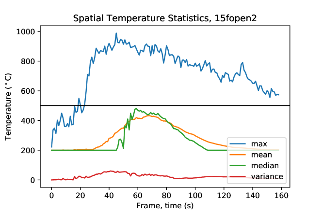
We start by computing basic spatial statistics of a time series of images: the mean, median, maximum, and standard deviation of the temperature values of each frame. To illustrate the typical behavior, in Figure 1 we plot these quantities for the dataset 15fopen2, a prescribed fire from 2015 in a longleaf pine flatwoods forest plot with no trees in the field of view. As the IR camera was calibrated to measure temperatures above 200°C, the results are determined with this background rather than ambient temperature. For this particular fire, there is a sudden increase in the mean and maximum temperature near $t=20$s which indicates that a significant number of pixels have ignited. We use the maximum temperature achieved at this time, about 500°C, to define a threshold between the burning and non-burning states. The choice is somewhat arbitrary in the sense that heterogeneous fuels imply a range of ignition temperatures; other choices are possible but lead to similar results.

Figure 1: Basic temperature statistics of a single dataset (15fopen2). The IR camera is calibrated to measure temperatures above 200°C. The black line indicates a temperature of 500°C that we use to distinguish between burning and non-burning pixels.

2.2 Pixel Burn Times

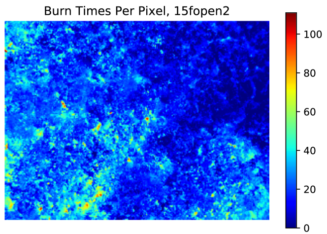
With a value separating burning and non-burning states, we can compute the burn time of each pixel for the same burn. Figure 2 shows the number of time steps that each pixel was above the 500°C threshold. Our estimates of burn time are directly relevant to the fire spread rate since longer burning time can overcome low probability of ignition and maintain fire spread. For instance, Almeida and Macau’s stochastic model [5] contains a universal parameter for the probability that a pixel burns (their “B”), which is a representation of the burn time, and this exerts an important control on fire spread in their model.

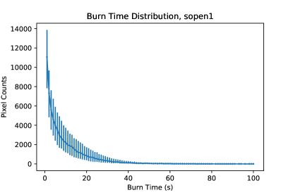
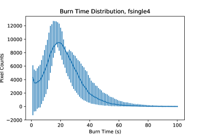
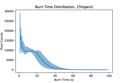
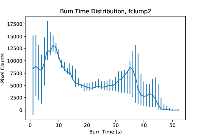
In addition to spatial maps of pixel burn times, we present burn time distributions of the 40 datasets. These distributions can be organized into four general trends, and representative distributions from each group are shown (Figure 3). The error is estimated with a $\pm 50^{\circ}$C range on the defined burn threshold. Note that the maximum burn time in the bottom right distribution is about half the size of the other three distributions. These distributions are described further Section 5.

Figure 2: The burn times for each pixel using a 500^∘C threshold. The colors indicate the number of time steps that each pixel burned.

Figure 3: Four burn time distributions with $50^{\circ}$C error bars that are representatives of the 40 datasets. Top left: A burn time distribution with exponential decay with an $e$-folding time of approximately four seconds. This is the most common distribution and can be found in twenty-four of our datasets. Top Right: Burn time distribution with a characteristic single peak in the distribution. This behavior is found in six of our datasets. Bottom Left: Burn time distribution with the characteristic of leveling off for several seconds before decreasing roughly exponentially. This behavior is found in eight of our datasets, including the dataset 15fopen2 in Figures 1 and 2. Bottom Right: Burn time distribution with the bi-modal characteristic of two distinct peaks in the burn time distribution. Only one fire shows this characteristic.

2.3 Probability of Spread

Another key parameter of a CA model is the probability of spread. We compute probabilities of a pixel igniting when any number of its nearest eight neighbors are on fire. Spotting can be included by defining the nearest neighbors to include additional layers of nearby pixels. In this work, however, we will coarsen the grid by aggregating pixels (Section 4), and this has the effect of reducing the amount of spotting.

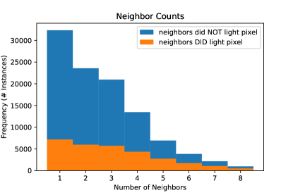
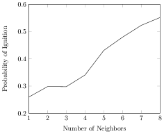
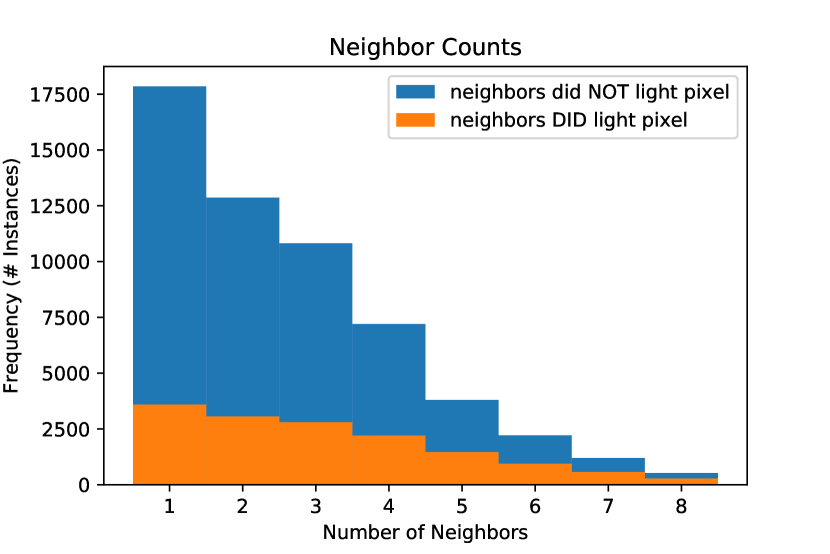
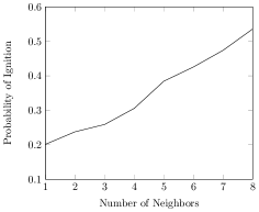
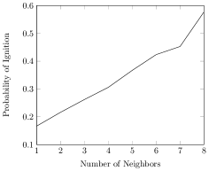
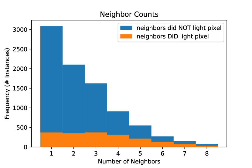
To calculate the probability of a fire spreading between pixels, we first identify pixels that are newly ignited in each frame. For each of these pixels, we count the number of nearest neighbors that were on fire. This gives a statistic of the likelihood of a pixel igniting given the condition that some number of its neighbors are burning. We can perform the same count for pixels that did not ignite when at least one of its neighbors was on fire. We plot these two values as a histogram in the left side of Figure 4. We exclude the case of newly ignited pixels where zero neighbors were on fire since this corresponds to spotting, a phenomenon that we are not investigating in this analysis. In the right plot of Figure 4, the histogram is used to compute the distribution of a pixel igniting.

Figure 4: Left: The number of instances where an unburnt pixel’s nearest neighbors did (orange) and did not (blue) cause ignition. Right: The probability of a pixel igniting conditioned on the number of its neighbors being on fire. For example, if four of an unburnt pixel’s neighbors are on fire, then it has approximately a 35% chance of igniting at the next time step.

3 A Simple Model for Fire Spread

A factor in fire spread that we have not explicitly treated in this analysis is wind. Wind can be modelled in a CA code by choosing probabilities of one pixel igniting another that are directionally dependent. For example, if there is no wind, then every burning neighbor of an unburnt pixel has the same probability of igniting this pixel. However, if there is a strong eastward wind then the burning neighbors to the left are the most likely to ignite an unburnt pixel.

We propose a basic two parameter model to understand the effect of the wind on the data. The parameters are the following.

1. $M$ is the number of neighbors that have the ability of igniting an unburnt pixel.

2. $p$ is the probability that one of these neighbors ignites an unburnt pixel.

The two extreme cases are $M=1$, where only one neighbor can ignite a pixel (high wind case), and $M=8$ where any pixel can ignite a neighboring pixel (no wind case). We let $X$ be the event of an unburnt pixel igniting at the next time step and $Y$ be the number of neighbors of this unburnt pixel that are currently burning. For a fixed $p$ and $M$, we are interested in computing $p(X\>|\>Y=N)$ which is the probability that an unburnt pixel ignites, given that it currently has $N$ burning neighbors.

These probabilities can be computed analytically. For example, if only one neighbor can ignite a pixel ($M=1$), then

$$p(X\>|\>Y=N)=\frac{N}{8}p.$$

In the other extreme, if any neighbor can ignite a pixel ($M=8$), then

$$p(X\>|\>Y=N) =\left(1+(1-p)+\cdots+(1-p)^{N-1}\right)p$$

$$=\frac{1-(1-p)^{N}}{1-(1-p)}p$$

$$=1-(1-p)^{N}.$$

The expressions for these probabilities become unwieldy for other values of $M$, so we use a Monte-Carlo approach to compute the probabilities. For a fixed $M$, $p$, and $N$, $10^{6}$ randomly selected configurations of burning neighbors are chosen, and for each burning neighbor that is able to ignite the unburnt pixel, we draw a random number to determine if the unburnt pixel is ignited. This method is verified with analytic expressions for the probabilities with $M=2$ and $M=3$ (not reported in this paper).

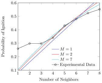
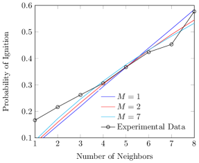
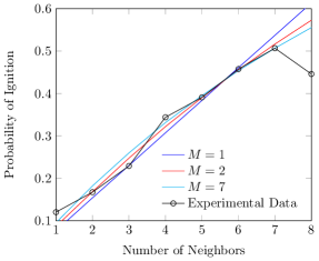
To find the best possible probability for each value of $M$, we compute the value of $p$ that minimizes the root mean square (RMS) for $N=1,\ldots,8$ between the Monte-Carlo method and the experimental data in Figure 4. This is done by choosing the optimal $p$ at an equispaced partitioning of $[0,1]$, and then using the value of $p$ that minimizes the RMS to choose lower and upper limits for a new search region. We iterate this procedure until the first two digits of the RMS is unchanging. For each value of $M$, we report the best probability of spread $p$ and the RMS value in Table 1. In Figure 5, we plot the experimental data and the best model fits when $M=1,2,7$. The other values of $M$ are similar to $M=7$. While the smallest RMS value is achieved when seven neighbors can ignite an unburnt pixel, this RMS value is comparable to other simulations where fewer neighbors have the ability to ignite a pixel. In particular, even if only 3 pixels can ignite an unburnt pixel, a RMS of almost 20% can be achieved for experimental data from complex dynamics with a very simple CA model. Further discussion of this behavior is described in Section 5.

$M$	$p$	RMS
1	0.6394	0.2563
2	0.3772	0.2139
3	0.2671	0.2016
4	0.2059	0.1952
5	0.1679	0.1928
6	0.1402	0.1897
7	0.1192	0.1885
8	0.1100	0.1891

Table 1: The best probability of spread $p$ for each choice of the number $M$ of neighbors that can ignite an unburnt pixel. Also reported is the root mean square error.

Figure 5: The probabilities of ignition for a different number of neighbors that can ignite an unburnt pixel (solid lines). The circled line is the experimental data from Figure 4.

4 Pixel Aggregation

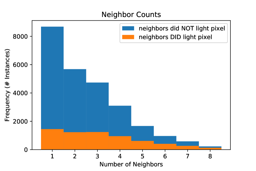
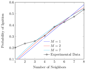
By only using the eight nearest neighbors as potential ignition sources for an unburnt pixel, we are ignoring ignition due to spotting. Given the spatial resolution of 1cm² of the IR images, it is unreasonable to assume that fire spreads to only its neighboring pixels at the 1 Hz speed of the camera. In reality, spotting occurs due to radiative and convective transport of heat, or by transport of an ember. To investigate the effect of spotting and to examine the fire dynamics at larger spatial scales, we aggregate groups of $3\times 3$, $5\times 5$, and $10\times 10$ pixels. We use the maximum temperature of the pixels in the aggregate to assign a temperature to the aggregate. The maximum value is used instead of the mean since the mean would be skewed by the 200°C threshold of the IR camera. We repeat the statistics reported in Figure 4 for these new aggregated pixels, and the results are in Figure 6.

We also repeat our probabilistic model for the aggregated pixel data sets. As before, for each number $M$ of pixels that can ignite an unburnt neighbor, we find the probability $p$ that minimizes the RMS over the number of burning neighbors $N$. For the $10\times 10$ aggregation, we do not include the $N=8$ entry in the RMS as this value seems to be an outlier which is feasible since there are very few instances when a $10\times 10$ unburnt aggregated pixel has 8 burning neighbors (see Figure 6(e)). The model fits are in Figure 7 and the optimal probabilities and RMS are in Table 2.

5 Discussion

Empirical data is needed to validate and inform new modelling tools in wildland fire [7]. Cellular automata codes rely on probabilistic rules to determine fire dynamics, and we have used 40 IR datasets from controlled burns to analyze two of the main parameters common in fire modeling using CA methods. We have focused on the burn times of a pixel and the probability of a unburnt pixel being ignited by its burning neighbors. We also analyzed the effect of the spatial resolution on these probabilities. Finally, we compared a simple model for fire spread to the experimental data at different aggregate resolutions.

First, the burn times depend strongly on the fuel type, moisture, wind speed, and other factors [10], but we found that from these 40 datasets, the burn times could be binned into four distributions plotted in Figure 3. Most of the datasets’ burn times have a distribution with a small mean (only a few seconds) and exponential decay (top left). This corresponds to a fast burning homogeneous fuel type. Another set of fire observations are represented by a mean closer to 20 seconds with an exponential decay (top right). This corresponds to a slower burning homogeneous fuel type. The third distribution (bottom left) has both a slow burning and fast burning fuels which indicates a heterogeneous fuel type. Finally, a single data set has a distribution with a large variance and a shorter maximum burn time (bottom right), and this corresponds to an even more heterogeneous fuel type. The 40 datasets have several variables, including the density of the trees and the moisture of the vegetation. Most of the datasets whose distribution resembles the top left plot of Figure 3 come from the drier vegetation, while the all of the datasets that resemble top right plot are from plots with a wetter vegetation.

One conclusion that our analysis reveals is that a single parameter for the burn time probability—many CA models make this assumption—is not applicable since the burn time distributions are wide. However, these prior burn time distributions (Figure 3) can be improved by using the experimental data to create a posterior distribution. That is, by using a Bayesian approach, the burn times, which are related to the fuel type, can be incorporated.

The probability of spread is described in terms of the number of burning neighbors. That is, given a newly ignited pixel, we determine how many of its neighbors are burning at the previous time step. The most common occurring instance is only one burning neighbor, while eight burning neighbors happens less frequently. To analyze these probabilities for larger grids, we aggregated pixels and computed the same probabilities. At all the resolutions we observed that most pixels are ignited by only one burning neighbor, while the fewest are ignited by eight neighbors. Moreover, the probability of ignition (right plots of Figures 4 and 6) verify, unsurprisingly, that the probability of ignition increases with the number of burning neighbors, and this probability distribution is essential for a CA model.

More interestingly, a simple model for fire spread captures features of these transition probabilities. First, for the unaggregated pixels (Figure 5), the model does a good job of capturing the experimental data when there are three or more burning neighbors. However, the model severely underestimates the probability of spread if only one or two neighbors are burning. In this case, we expect that much of the fire spread is nonlocal from convective heating and small-scale spotting, and our model does not account for these nonlocal effects. This hypothesis is further supported by analyzing the aggregated cells. In these cases, the effective spotting becomes less prevalent, and we expect that the leading cause of new ignition is neighboring pixels.

In Figure 7 and Table 2, we see that the fit between the model and the experimental data improves as larger pixels are considered. In particular, an RMS of less than 5% is achieved when considering pixels that are 10cm². This suggests that the resolution of the camera was high enough to observe the fine scale processes of combustion and that some averaging over these processes is needed to produce stable statistics of fire spread, a result that was confirmed by Loudermilk et al. [12]. The degree of averaging necessary was found to be 10cm² in these experiments.

The spatial structure of burn times (e.g. Figure 2) is a small-scale example of the fuel bed complexity that can result from even the simplest of rules. For instance [20] describes a simulated tree population model with instantaneous fire spread and zero burn time. Real wildland systems have finite spread rate but their model shows how the fuel itself (they simulated trees but it could be any fuel) can spontaneously develop complex spatial structure.

Differentiating between the three prevalent types of fire (i.e. head fire, backing fire, and flanking fire) is important because the different types of fire have different probabilities for spreading. With a similar statistical analysis we can differentiate these different types of fire spread with the appropriate images, we will be able to further constrain these probabilities and use them to build models with more intrinsic fidelity to fire propagation, and fewer unknown parameters, leading to more accurate predictions.

(a) $3\times 3$ aggregated groups.

(b) $3\times 3$ aggregated groups.

(c) $5\times 5$ aggregated groups.

(d) $5\times 5$ aggregated groups.

(e) $10\times 10$ aggregated groups.

(f) $10\times 10$ aggregated groups.

Figure 6: Left: The number of instances where an unburnt aggregated pixel’s nearest neighbors did (orange) and did not (blue) cause ignition at different levels of aggregation. Right: The probability of an aggregated pixel igniting conditioned on the number of its aggregated neighbors being on fire.

$M$	$p$	RMS
1	0.5779	0.1734
2	0.3321	0.1459
3	0.2339	0.1355
4	0.1810	0.1333
5	0.1436	0.1301
6	0.1247	0.1296
7	0.1061	0.1284
8	0.0948	0.1287

(a) $3\times 3$ aggregated groups.

$M$	$p$	RMS
1	0.5843	0.1389
2	0.3256	0.1111
3	0.2306	0.1052
4	0.1765	0.1005
5	0.1378	0.1001
6	0.1188	0.0956
7	0.1028	0.0959
8	0.0896	0.0938

(b) $5\times 5$ aggregated groups.

$M$	$p$	RMS
1	0.6137	0.0643
2	0.3463	0.0443
3	0.2403	0.0426
4	0.1825	0.0432
5	0.1498	0.0406
6	0.1261	0.0436
7	0.1090	0.0436
8	0.0956	0.0450

(c) $10\times 10$ aggregated groups.

Table 2: The best probability of spread $p$ for each choice of the number $M$ of neighbors that can ignite an unburnt aggregated pixel. Also reported is the root mean square error.

(a) $3\times 3$ aggregated groups.

(b) $5\times 5$ aggregated groups.

(c) $10\times 10$ aggregated groups.

Figure 7: The probabilities of ignition for a different number of neighbors that can ignite an unburnt pixel (solid lines). The circled line is the experimental data from Figure 6.

References

- [1] Gary L. Achtemeier. ”Rabbit Rules” – An Application of Stephen Wolfram’s “New Kind of Science” to Fire Spread Modeling. In Fifth symposium on fire and forest meteorology, pages 16–20, 2003.
- [2] Gary L. Achtemeier. Planned Burn-Piedmont. A local operational numerical meteorological model for tracking smoke on the ground at night: model development and sensitivity tests. International Journal of Wildland Fire, 14(1):85–98, 2005.
- [3] Gary L. Achtemeier. Field validation of a free-agent cellular automata model of fire spread with fire–atmosphere coupling. International Journal of Wildland Fire, 22:148–156, 2013.
- [4] G. Albinet, G. Searby, and D. Stauffer. Fire propagation in a 2-D random medium. Journal de Physique, 47(1):1–7, 1986.
- [5] Rodolfo Maduro Almeida and Elbert Einstein Nehrer Macau. Stochastic Cellular Automata Model for Wildland Fire Spread Dynamics. Journal of Physics: Conference Series, 285(1):012038, 2011.
- [6] Keith C. Clarke, James A. Brass, and Phillip J. Riggan. A cellular automaton model of wildfire propagation and extinction. Photogrammetric Engineering & Remote Sensing, 60(11):1355–1367, 1994.
- [7] Miguel G. Cruz, Martin E. Alexander, and Andrew L. Sullivan. Mantras of wildland fire behaviour modelling: facts or fallacies? International Journal of Wildland Fire, 26(11):973–981, 2017.
- [8] Nathan Dahl, Haidong Xue, Xiaolin Hu, and Ming Xue. Coupled fire–atmosphere modeling of wildland fire spread using DEVS-FIRE and ARPS. Natural Hazards, 77(2):1013–1035, 2015.
- [9] J. A. M. S. Duarte. Bushfire Automata and Their Phase Transitions. International Journal of Modern Physics C, 8(02):171–189, 1997.
- [10] Eunmo Koo, Patrick Pagni, John Woychesse, Scott Stephens, David Weise, and Jeremy Huff. A Simple Physical Model for Forest Fire Spread Rate. Fire Safety Science, 8:851–862, 2005.
- [11] Rodman Linn, Jon Reisner, Jonah J. Colman, and Judith Winterkamp. Studying wildfire behavior using FIRETEC. International Journal of Wildland Fire, 11(4):233–246, 2002.
- [12] E. Louise Loudermilk, Gary L. Achtemeier, Joseph J. O’Brien, J. Kevin Hiers, and Benjamin S. Hornsby. High-resolution observations of combustion in heterogeneous surface fuels. International Journal of Wildland Fire, 23:1016–1026, 2014.
- [13] Hussam Mahmoud and Akshat Chulahwat. A Probabilistic Cellular Automata Framework for Assessing the Impact of WUI Fires on Communities. Procedia Engineering, 198:1111–1122, 2017.
- [14] J. Margerit and O. Séro-Guillaume. Richards’ model, Hamilton-Jacobi equation and temperature field equations of forest fires. In Proceedings of the III International Conference on Forest Fire Research and 14th Conference on Fire and Forest Meteorology, volume 1, pages 281–294, 1998.
- [15] Vicenç Méndez and Josep E Llebot. Hyperbolic reaction-diffusion equations for a forest fire model. Physical Review E, 56(6):6557, 1997.
- [16] Vasileios G. Ntinas, Byron E. Moutafis, Giuseppe A. Trunfio, and Georgios Ch. Sirakoulis. Parallel fuzzy cellular automata for data-driven simulation of wildfire spreading. Journal of Computational Science, 21:469–485, 2017.
- [17] Joseph J. O’Brien, E. Louise Loudermilk, Benjamin Hornsby, Andrew T. Hudak, Benjamin C. Bright, Matthew B. Dickinson, J. Kevin Hiers, Casey Teske, and Roger D. Ottmar. High-resolution infrared thermography for capturing wildland fire behaviour: RxCADRE 2012. International Journal of Wildland Fire, 25(1):62–75, 2016.
- [18] Gwynfor D. Richards. An elliptical growth model of forest fire fronts and its numerical solution. International Journal for Numerical Methods in Engineering, 30(6):1163–1179, 1990.
- [19] Richard C. Rothermel. A mathematical model for predicting fire spread in wildland fuels. USDA Forest Service research paper INT, 115, 1972.
- [20] K. Schenk, B. Drossel, S. Clar, and F. Schwabl. Finite-size effects in the self-organized critical forest-fire model. The European Physical Journal B-Condensed Matter and Complex Systems, 15(1):177–185, 2000.
- [21] A. Sullivan. Wildland surface fire spread modelling, 1990-2007. 3: Simulation and mathematical analogue models. International Journal of Wildland Fire, 18:387–403, 2009.
- [22] A.L. Sullivan and I.K. Knight. A hybrid cellular automata/semi-physical model of fire growth. In Proceedings of the Seventh Asia-Pacific Conference on Complex Systems, pages 6–10, 2004.
- [23] Giuseppe A. Trunfio, Donato D’Ambrosio, Rocco Rongo, William Spataro, and Salvatore Di Gregorio. A New Algorithm for Simulating Wildfire Spread through Cellular Automata. ACM Transactions on Modeling and Computer Simulation, 22(1):6, 2011.
- [24] S.D. Watt, A.J. Roberts, and R.O. Weber. Dimensional reduction of a bushfire model. Mathematical and Computer Modelling, 21(9):79–83, 1995.
- [25] Stephen Wolfram. Statistical mechanics of cellular automata. Reviews of Modern Physics, 55(3):601–644, 1983.