Learning a Complete Image Indexing Pipeline

Abstract

To work at scale, a complete image indexing system comprises two components: An inverted file index to restrict the actual search to only a subset that should contain most of the items relevant to the query; An approximate distance computation mechanism to rapidly scan these lists. While supervised deep learning has recently enabled improvements to the latter, the former continues to be based on unsupervised clustering in the literature. In this work, we propose a first system that learns both components within a unifying neural framework of structured binary encoding.

1 Introduction

Decades of research have produced powerful means to extract features from images, effectively casting the visual comparison problem into one of distance computations in abstract spaces. Whether engineered or trained using convolutional deep networks, such vector representations are at the core of all content-based visual search engines. This applies particularly to example-based image retrieval systems where a query image is used to scan a database for images that are similar to the query in some way: in that they are the same image but one has been edited (near duplicate detection), or because they are images of the same object or scene (instance retrieval), or because they depict objects or scenes from the same semantic class (category retrieval).

Deploying such a visual search system requires conducting nearest neighbour search in a high-dimensional feature space. Both the dimension of this space and the size of the database can be very large, which imposes severe constraints if the system is to be practical in terms of storage (memory footprint of database items) and of computation (search complexity). Exhaustive exact search must be replaced by approximate, non-exhaustive search. To this end, two main complementary methods have emerged, both relying on variants of unsupervised vector quantization (VQ). The first such method, introduced by Sivic and Zisserman [25] is the inverted file system. Inverted files rely on a partitioning of the feature space into a set of mutually exclusive bins. Searching in a database thus amounts to first assigning the query image to one or several such bins, and then ranking the resulting shortlist of images associated to these bins using the Euclidean distance (or some other distance or similarity measure) in feature space.

The second method, introduced by Jegou et al. [15], consists of using efficient approximate distance computations as part of the ranking process. This is enabled by feature encoders producing compact representations of the feature vectors that further do not need to be decompressed when computing the approximate distances. This type of approaches, which can be seen as employing block-structured binary representations, superseded the (unstructured) binary hashing schemes that dominated approximate search.

Despite its impressive impact on the design of image representations [11, 1, 10, 23], supervised deep learning is still limited in what concerns the approximate search system itself. Most recent efforts focus on supervised deep binary hashing schemes, as discussed in the next section. As an exception, the work of Jain et al. [13] employs a block-structured approach inspired by the successful compact encoders referenced above. Yet the binning mechanisms that enable the usage of inverted files, and hence large-scale search, have so far been neglected.

In this work we introduce a novel supervised inverted file system along with a supervised, block-structured encoder that together specify a complete, supervised, image indexing pipeline. Our design is inspired by the two methods of successful indexing pipelines described above, while borrowing ideas from [13] to implement this philosophy.

Our main contributions are as follows: (1) We propose the first, to our knowledge, image indexing system to reap the benefits of deep learning for both data partitioning and feature encoding; (2) Our data partitioning scheme, in particular, is the first to replace unsupervised VQ by a supervised approach; (3) We take steps towards learning the feature encoder and inverted file binning mechanism simultaneously as part of the same learning objective; (4) We establish a wide margin of improvement over the existing baselines employing state-of-the art deep features, feature encoders and binning mechanism.

2 Background

Approximating distances through compact encoding

Concerning approximate distance computations, two main approaches exist. Hashing methods [26], on the one hand, employ Hamming distances between binary hash codes. Originally unsupervised, these methods have recently benefited from progress in deep learning [27, 28, 30, 17, 18, 19, 7], leading to better systems for category retrieval in particular. Structured variants of VQ, on the other hand, produce fine-grain approximations of the high-dimensional features themselves through very compact codes [3, 8, 9, 12, 15, 16, 20, 29] that enable look-up table-based efficient distance computations. Contrary to recent hashing methods, VQ-based approaches have not benefited from supervision so far. However, Jain et al. [13] recently proposed a supervised deep learning approach that leverages the advantages of structured compact encoding and yields state-of-the-art results on several retrieval tasks. Our work extends this supervised approach towards a complete indexing pipeline, that is, a system that also includes an inverted file index.

Scanning shorter lists with inverted indexes

For further efficiency, approximate search is further restricted to a well chosen fraction of the database. This pruning is carried out by means of an Inverted File (IVF), which relies on a partitioning of the feature space into Voronoi cells defined using $K$-means clustering [14, 2]. Two things should be noted: The method to build the inverted index is unsupervised and it is independent from the way subsequent distance approximations are conducted (e.g., while VQ is used to build the index, short lists can be scanned using binary embeddings [14]). In this work, we propose a unifying supervised framework. Both the inverted index and the encoding of features are designed and trained together for improved performance. In the next section, we expose in more detail the existing tools to design IVF/approximate search pipelines, before moving to our proposal in Section 4.

3 Review of image indexing

Image indexing systems are based on two main components: (i) an inverted file and (ii) a feature encoder. In this section we describe how these two main components are used in image indexing systems, thus laying out the motivation for the method we introduce in §4.

Inverted File (IVF)

An inverted file relies on a partition of the database into mutually exclusive bins, a subset of which is searched at query time. The partitioning is implemented by means of VQ [25, 15, 2]: Given a vector $\bm{x}\in\mathbb{R}^{d}$ and a codebook $\bm{D}=[\bm{d}_{k}\in\mathbb{R}^{d}]_{k=1}^{N}$, the VQ representation of $\bm{x}$ in $\bm{D}$ is obtained by solving

$$n=\operatorname*{argmin}\nolimits_{k}\|\bm{x}-\bm{d}_{k}\|_{2}^{2},$$ (1)

where $n$ is the codeword index for $\bm{x}$ and $\bm{d}_{n}$ its reconstruction. Given a database $\{\bm{x}_{i}\}_{i}$ of image features, and letting $n_{i}$ represent the codeword index of $\bm{x}_{i}$, the database is partitioned into $N$ index bins $\mathcal{B}_{n}$. These bins, stored along with metadata that may include the features $\bm{x}_{i}$ or a compact representation thereof, is known as an inverted file. At query time, the bins are ranked by decreasing pertinence $n_{1},\ldots,n_{N}$ relative to the query feature $\bm{x}^{*}$ so that

$$\|\bm{x}^{*}-\bm{d}_{n_{1}}\|\leq\ldots\leq\|\bm{x}^{*}-\bm{d}_{n_{N}}\|,$$ (2)

i.e., by increasing order of reconstruction error. Using this sorting, one can specify a target number of images $T$ to retrieve from the database and search only the first $B$ bins so that $\sum_{k=1}^{B-1}\left|\mathcal{B}_{n_{k}}\right|\leq T\leq\sum_{k=1}^{B}\left|\mathcal{B}_{n_{k}}\right|$.

It is important to note that all existing state-of-the-art indexing methods employ a variant of the above described mechanism that relies on $K$-means-learned codebooks $\bm{D}$. To the best of our knowledge, ours is the first method to reap the benefits of deep learning to build an inverted file.

Feature encoder

The inverted file outputs a shortlist of images with indices in $\bigcup_{k=1}^{B}\mathcal{B}_{n_{k}}$, which needs to be efficiently ranked in terms of distance to the query This is enabled by compact feature encoders that allow rapid distance computations without decompressing features. It is important to note that the storage bitrate of the encoding affects – besides storage cost – search speed, as higher bitrates means that bins need to be stored in secondary storage, where look-up speeds are a significant burden.

State-of-the art image indexing systems use feature encoders that employ a residual approach: A residual is computed from each database feature $\bm{x}$ and its reconstruction $\bm{d}_{n}$ obtained as part of the inverted file bin selection in (1):

$$\bm{r}_{n}=\bm{x}-\bm{d}_{n}.$$ (3)

This residual is then encoded using a very high resolution quantizer. Several schemes exist [6, 15] that exploit structured quantizers to enable low-complexity, high-resolution quantization, and herein we describe product quantizers and related variants [15, 20, 8]. Such vector quantizers employ a codebook $\bm{C}\in\mathbb{R}^{d\times K^{M}}$ with codewords that are themselves additions of codewords from $M$ smaller constituent codebooks $\bm{C}_{m}=\left[\bm{c}_{m,k}\right]_{k}\in\mathbb{R}^{d\times K},m=1,\ldots,M$, that are orthogonal ($\forall m\neq l,\bm{C}_{m}^{\textrm{T}}\bm{C}_{l}=\bm{0}$):

$$\bm{C}=\Big{[}\sum\nolimits_{m=1}^{M}\bm{c}_{m,k_{m}}\Big{]}_{(k_{1},\ldots,k_{M})\in(1,\ldots,K)^{M}}.$$ (4)

Accordingly, an encoding of $\bm{r}$ in this structured codebook is specified by the indices $(k_{1},\ldots,k_{M})$ which uniquely define the codeword $\bm{c}$ from $\bm{C}$, i.e., the reconstruction of $\bm{r}$ in $\bm{C}$. Note that the bitrate of this encoding is $M\log_{2}(K)$.

Asymmetric distance computation

Armed with such a representation for all database vectors, one can very efficiently compute an approximate distance between a query $\bm{x}^{*}$ and all database features $\bm{x}\in\{\bm{x}_{i},i\in\cup_{k=1}^{B}\mathcal{B}_{n_{k}}\}$ in top-ranked bins. The residual of $\bm{x}^{*}$ for bin $\mathcal{B}_{n}$ is

$$\bm{r}_{n}^{*}=\bm{x}-\bm{d}_{n}$$ (5)

and the approach is asymmetrical in that this uncompressed residual is compared to the compressed, reconstructed residual representation $\bm{c}$ of the database vectors $\bm{x}$ in bin $\mathcal{B}_{n}$ using the distance

$$\|\bm{r}_{n}^{*}-\bm{c}\|_{2}^{2}=\sum_{m=1}^{M}\|\bm{r}_{n}^{*}-\bm{c}_{m,k_{m}}\|_{2}^{2}.$$ (6)

We define the look-up tables (LUT)

$$\bm{z}_{n,m}\triangleq\left[\;\|\bm{r}_{n}^{*}-\bm{c}_{m,k}\|_{2}^{2}\;\right]_{k}\in\mathbb{R}^{K}$$ (7)

containing the distances between $\bm{r}_{n}^{*}$ and all codewords of $\bm{C}_{m}$. Building these LUTs enables us to compute (6) using $\sum_{m=1}^{M}\bm{z}_{m}[k_{m}]$, an operation that requires only $M$ table look-ups and additions, establishing the functional benefit of the encoding $(k_{1},\ldots,k_{M})$.

To gain some insight into the above encoding, consider the one-hot representation $\bm{b}_{m}$ of the indices $k_{m}$ given by

$$\bm{b}_{m}=\big{[}\llbracket l=k_{m}\rrbracket\big{]}_{l}\in\mathcal{K}_{K},$$ (8)

where $\llbracket\cdot\rrbracket$ denotes the Iverson brackets and

$$\mathcal{K}_{K}\triangleq\{\bm{a}\in\{0,1\}^{K},\|\bm{a}\|_{1}=1\}.$$ (9)

Using stacked column vectors

$$\bm{b} =\textsc{{col}}\left(\bm{b}_{1},\ldots,\bm{b}_{M}\right)\in\mathcal{K}_{K}^{M}\textrm{ and }$$ (10)

$$\bm{z}_{n} =\textsc{{col}}\left(\bm{z}_{n,1},\ldots,\bm{z}_{n,M}\right)\in\mathbb{R}_{+}^{MK},$$ (11)

distance (6) can be expressed as follows:

$$\|\bm{r}_{n}^{*}-\bm{c}\|_{2}^{2}=\bm{z}_{n}^{\textrm{T}}\bm{b}.$$ (12)

Namely, computing approximate distances between a query $\bm{x}^{*}$ and the database features $\bm{x}\in\{\bm{x}_{i},i\in\mathcal{B}_{n}\}$ amounts to computing an inner-product between a bin-dependent mapping $\bm{z}_{n}\in\mathbb{R}^{MK}$ of the query feature $\bm{x}^{*}$ and a block-structured binary code $\bm{b}\in\mathcal{K}_{M}^{K}$ derived from $\bm{x}$. A search then consists of computing all such approximate distances for the $B$ most pertinent bins and then sorting the corresponding images in increasing order of these distances.

It is worth noting that most of the recent supervised binary encoding methods [27, 28, 30, 17, 18, 19, 7] do not use structured binary codes of the form $\bm{b}$ in (12). The main exception being SuBiC [13], which further uses a sorting score that is an inner product of the same form as (12).

4 A complete indexing pipeline

The previous section established how state-of-the-art large-scale image search systems rely on two main components: an inverted file and a functional residual encoder that produces block-structured binary codes. While compact binary encoders based on deep learning have been explored in the literature, inverted file systems continue to rely on unsupervised $K$-means codebooks.

In this section we first revisit the SuBiC encoder [13], and then show how it can be used to implement a complete image indexing system that employs deep learning methodology both at the IVF stage and compact encoder stage.

4.1 Block-structured codes

Figure 1: The SuBiC encoder operates on the feature vector $\bm{x}$ produced by a CNN to enable learning of (relaxed) block-structured codes ($\tilde{\bm{b}}$) $\bm{b}$. Blue, yellow, and green blocks are active, respectively, only at training time, only at testing time and at training/testing times.

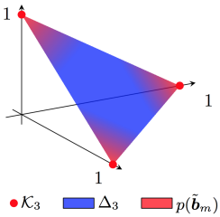
Figure 2: The discrete set $\mathcal{K}_{3}$ of one-hot encoded vectors, its convex-hull $\Delta_{3}$, and the distribution of relaxed blocks $\tilde{\bm{b}}_{m}$ enforced by the SuBiC entropy losses. Omitting the negative batch entropy loss (19) would result in situations where $p(\tilde{\bm{b}}_{m})$ is concentrated near only $k<3$ of the elements in $\mathcal{K}_{3}$.

Figure 3: Proposed indexing architecture. The proposed indexing architecture consists of a bin selection component, a residual computation component, and a feature encoder. We use blocks with square corners (labeled with a weights matrix) to denote fully-connected linear operations, potentially followed by a ReLU or softmax (SM) nonlinearity. Blue, yellow, and green blocks are active, respectively, only at training time, only at testing (i.e. database indexing / querying) time and at training/testing times. The residual block can be disabled to define a new architecture, as illustrated by the switch at the bottom of the diagram.

The SuBiC encoder in Fig. 1 was the first to leverage supervised deep learning to produce a block-structured code of the form $\bm{b}\in\mathcal{K}_{K}^{M}$ in (10). At learning time, the method relaxes the block-structured constraint. Letting

$$\Delta_{K}=\big{\{}\bm{a}\in\mathbb{R}_{+}^{K}\textrm{ s.t. }\sum\nolimits_{k}\bm{a}[k]=1\big{\}}$$ (13)

denote the convex hull of $\mathcal{K}_{K}$, said relaxation

$$\tilde{\bm{b}}\in\Delta_{K}^{M}$$ (14)

is enforced by means of a fully-connected layer of output size $KM$ and ReLU activation with output $\bm{z}$ that is fed to a block softmax non-linearity that operates as follows: Let $\bm{z}_{m}$ denote the $m$-th block of $\bm{z}\in\mathbb{R}^{KM}$ such that $\bm{z}=\textsc{{col}}\left(\bm{z}_{1},\ldots,\bm{z}_{M}\right)$. Likewise, let $\tilde{\bm{b}}_{m}\in\Delta_{K}$ denote the $m$-th block of the relaxed code $\tilde{\bm{b}}\in\Delta_{K}^{M}$. The block softmax non-linearity operates by applying a standard softmax non-linearity to each block $\bm{z}_{m}$ of $\bm{z}$ to produce the corresponding block $\tilde{\bm{b}}_{m}$ of $\tilde{\bm{b}}$:

$$\tilde{\bm{b}}_{m}=\left[\frac{\exp\left(\bm{z}_{m}[k]\right)}{\sum_{l}\exp\left(\bm{z}_{m}[l]\right)}\right]_{k}.$$ (15)

At test time, the block-softmax non-linearity is replaced by a block one-hot encoder that projects $\tilde{\bm{b}}$ unto $\Delta_{K}^{M}$. In practice, this can be accomplished by means of one-hot encoding of the index of the maximum entry of $\bm{z}_{m}$:

$$\bm{b}_{m}=\big{[}\;\llbracket k=\operatorname*{argmax}(\bm{z}_{m})\rrbracket\;\big{]}_{k}.$$ (16)

The approach of [13] introduced two losses based on entropy that enforce the proximity of $\tilde{\bm{b}}$ to $\mathcal{K}_{K}^{M}$. The entropy of a vector $\bm{p}\in\Delta_{K}$, defined as

$$\textrm{E}(\bm{p})=\sum\nolimits_{k=1}^{K}\bm{p}[k]\log_{2}\left(\bm{p}[k]\right),$$ (17)

has a minimum equal to zero for deterministic distributions $\bm{p}\in\mathcal{K}_{K}$, motivating the use of the entropy loss

$$\ell_{\mathrm{E}}(\tilde{\bm{b}})\triangleq\sum\nolimits_{m=1}^{M}\textrm{E}(\tilde{\bm{b}}_{m})$$ (18)

to enforce the proximity of the relaxed blocks $\tilde{\bm{b}}_{m}$ to $\mathcal{K}_{K}$.This loss on its own, however, could lead to situations where only some elements of $\mathcal{K}_{K}$ are favored (c.f. Fig. 2), meaning that only a subset of the support of the $\bm{b}_{m}$ is used.

Yet entropy likewise has a maximum of $\log_{2}(K)$ for uniform distributions $\bm{p}=\frac{1}{K}\bm{1}$. This property can be used to encourage uniformity in the selection of elements of $\mathcal{K}_{K}$ by means of the negative batch entropy loss, computed for a batch $\mathcal{A}=\{\tilde{\bm{b}}^{(i)}\}_{i}$ of size $|\mathcal{A}|$ using

$$\ell_{\mathrm{B}}\left(\mathcal{A}\right)\triangleq-\sum\nolimits_{m=1}^{M}\textrm{E}\Big{(}\frac{1}{|\mathcal{A}|}\sum_{i}\tilde{\bm{b}}_{m}^{(i)}\Big{)}.$$ (19)

For convenience, we define the SuBiC loss computed on a batch $\mathcal{A}$ as the weighted combination of the two entropy losses, parametrized by the hyper-parameters $\mu,\gamma\in\mathbb{R}_{+}$:

$$\ell_{\mathrm{S}}^{\mu,\gamma}\big{(}\mathcal{A}\big{)}\triangleq\frac{\mu}{|\mathcal{A}|}\sum\nolimits_{\tilde{\bm{b}}\in\mathcal{A}}\ell_{\mathrm{E}}(\tilde{\bm{b}})+\gamma\ell_{\mathrm{B}}\left(\mathcal{A}\right).$$ (20)

It is important to point out that, unlike the residual encoder described in §3, the SuBiC approach operates on the feature vector $\bm{x}$ directly. Indeed, the SuBiC method is only a feature encoder, and does not implement an entire indexing framework.

4.2 A novel indexing pipeline

We now introduce our proposed network architecture that uses the method of [13] described above to build an entire image indexing system. The system we design implements the main ideas of the state-of-the-art pipeline described in §3.

Our proposed network architecture is illustrated in Fig. 3. The input to the network is the feature vector $\bm{x}$ consisting of activation coefficients obtained by running a given image $\bm{I}$ through a CNN feature extractor. We refer to this feature extractor as the base CNN of our system.

Similarly to the design philosophy described in §3, our indexing system employs an IVF and a residual feature encoder. Accordingly, the architecture in Fig. 3 consists of two main blocks, Bin selection and Encoder, along with a Residual block that links these two main components.

Bin selection

The first block, labeled Bin selection in Fig. 1 can be seen as a SuBiC encoder employing a single block (i.e. $M=1$) of size $N$, with the block one-hot encoder substituted by an argmax operation. The block consists of a single fully-connected layer with weight matrix $\bm{W}_{1}$ and ReLU activation followed by a second activation using softmax. When indexing a database image $\bm{I}$, this block is responsible for choosing the bin $\mathcal{B}_{n}$ that $\bm{I}$ is assigned to, using the argmax of the coefficients $\bm{z}^{\prime}$.

Given a query image $\bm{I}^{*}$, the same binning block is responsible for sorting the bins in decreasing order of pertinence $\mathcal{B}_{n_{1}}\cdots\mathcal{B}_{n_{N}}$ using the coefficients $\bm{z}^{\prime*}\in\mathbb{R}^{N}_{+}$ so that

$$\bm{z}^{\prime*}[n_{1}]\geq\ldots\geq\bm{z}^{\prime*}[n_{N}],$$ (21)

in a manner analogous to (2).

(Residual) feature encoding

Inspired by the residual encoding approach described in §3, we consider a block analogous to the residual computation of (3) and (5). The approach consists of building a vector (denoting ReLU as $\sigma$)

$$\bm{R}_{2}\sigma(\bm{R}_{1}\tilde{\bm{b}}^{\prime}),$$ (22)

that is analogous to the reconstruction $\bm{d}_{n}$ of $\bm{x}$ obtained from the encoding $n$ following the IVF stage (c.f. (1) and discussion thereof), and subtracts it from a linear mapping of $\bm{x}$:

$$\bm{r}=\bm{Q}\bm{x}-\bm{R}_{2}\sigma(\bm{R}_{1}\tilde{\bm{b}}^{\prime}).$$ (23)

Besides the analogy to indexing pipelines, one other motivation for the above approach is to provide information to the subsequent feature encoding from the IVF bin selection stage (i.e. $\tilde{\bm{b}}^{\prime}$) as well as the original feature $\bm{x}$. For completeness, as illustrated in Fig. 3, we also consider architectures that override this residual encoding block, setting $\bm{r}=\bm{x}$ directly.

The final stage consists of an $M$-block SuBiC encoder operating on $\bm{r}$ and producing test-time encodings $\bm{b}\in\mathcal{K}_{K}^{M}$, and training-time relaxed encoding $\tilde{\bm{b}}\in\Delta_{K}^{M}$. Note that, unlike the residual approach described in §3, our approach does not incurr the extra overhead required to compute LUTs using (7).

Searching

Given a query image $\bm{I}^{*}$, it is first fed to the pipeline in Fig. 3 to obtain (i) the activation coefficients $\bm{z}^{\prime*}$ at the output of the $\bm{W}_{1}$ layer and (ii) the activation coefficients $\bm{z}^{*}$ at the output of the $\bm{W}_{2}$ layer. The IVF bins are then ranked as per (21) and all database images $\big{\{}\bm{I}_{i},~{}i\in\bigcup_{k=1}^{B}\mathcal{B}_{n_{k}}\big{\}}$ in the $B$ most pertinent bins are sorted, based on their encoding $\bm{b}_{i}$, according to their score

$$\bm{z}^{\prime*{\textrm{T}}}\bm{b}_{i}.$$ (24)

Training

We assume we are given a training set $\{(\bm{I}^{(i)},y^{(i)})\}_{i}$ organized into $C$ classes, where label $y^{(i)}\in(1,\ldots,C)$ specifies the class of the $i$-th image. Various works on learning for retrieval have explored the benefit of using ranking losses like the triplet loss and the pair-wise loss as opposed to the cross-entropy loss succesfully used in classification tasks [11, 27, 28, 30, 17, 18, 19, 7, 5]. Empirically, we have found that the cross-entropy loss yields good results in the retrieval task, and we adopt it in this work.

Given an image belonging to class $c$ and a vector $\bm{p}\in\Delta_{C}$ that is an estimate of class membership probabilities, the cross-entropy loss is given by (the scaling is for convenience of hyper-parameter cross-validation)

$$\ell\left(\bm{p},c\right)=-\frac{1}{\log_{2}{C}}\log_{2}\bm{p}[c].$$ (25)

Accordingly, we train our network by enforcing that the relaxed block-structured codes $\tilde{\bm{b}}^{\prime}$ and $\tilde{\bm{b}}$ are good feature vectors that can be used to predict class membership. We do so by feeding each vector to a soft-max classification layer (layers $\bm{C}_{1}$ and $\bm{C}_{2}$ in Fig. 3, respectively), thus producing estimates of class membership $\bm{s}^{\prime}$ and $\bm{s}$ in $\Delta_{C}$ (c.f. Fig. 3) from which we derive two possible task-related losses. Letting $\mathcal{T}$ denote a batch specified as a set of training-pair indices, these two losses are

$$L_{1,\alpha}=\frac{1}{|\mathcal{T}|}\sum_{i\in\mathcal{T}}\Big{[}\alpha\ell\big{(}\bm{s}^{\prime(i)},y^{(i)}\big{)}+\ell\big{(}\bm{s}^{(i)},y^{(i)}\big{)}\Big{]}$$ (26)

$$\textrm{ and }L_{2}=\frac{1}{|\mathcal{T}|}\sum_{i\in\mathcal{T}}\ell\big{(}\bm{s}^{\prime(i)}+\bm{s}^{(i)},y^{(i)}\big{)},$$ (27)

where the scalar $\alpha\in\{0,1\}$ is a selector variable. In order to enforce the proximity of the $\tilde{\bm{b}}^{\prime}$ and $\tilde{\bm{b}}$ to $\mathcal{K}_{N}$ and $\mathcal{K}_{K}^{M}$, respectively, we further employ the loss

$$\Omega_{\mathcal{H}}=\ell_{\mathrm{S}}^{\mu_{1},\gamma_{1}}\big{(}\{\tilde{\bm{b}}^{\prime(i)}\}_{i\in\mathcal{T}}\big{)}+\ell_{\mathrm{S}}^{\mu_{2},\gamma_{2}}\big{(}\{\tilde{\bm{b}}^{(i)}\}_{i\in\mathcal{T}}\big{)},$$ (28)

which depends on the four hyper-parameters $\mathcal{H}=\{\mu_{1},\gamma_{1},\mu_{2},\gamma_{2}\}$ (we disuss heuristics for their selection if §5).

Accordingly, the general learning objective for our system is

$$F_{*}=L_{*}+\Omega_{\mathcal{H}},$$ (29)

and we consider three variants thereof:

(SuBiC-I) a non-residual variant with objective $F_{1,1}$ corresponding to independently training the bin selection block and the feature encoder;

(SuBiC-R) a residual variant with objective $F_{1,0}$ where the bin selection block is pre-trained and held fixed during learning; and

(SuBiC-J) a non-residual variant with objective $F_{2}$.

5 Experiments

Method	Oxford5K	Oxford5K*	Paris6K	Holidays	Oxford105K	Paris106K
DIR [11]	84.94	84.09	93.58	90.32	83.52	89.10
PQ [15]	46.57	39.45	57.57	48.23	38.73	42.23
SuBiC [13]	53.25	46.06	71.28	60.52	46.88	58.27

Table 1: Instance retrieval with encoded features. Performance (mAP) comparison using $64$-bit codes, first row shows reference results with original uncompressed features. When bounding box information is used for Oxford5K dataset, the performance degrades for both PQ and SuBiC, shown in column Oxford5K*, as both are trained on full images.

Figure 4: Large-scale image retrieval with complete pipelines Plots of mAP vs. (average) shortlist size $T$. For all methods except IMI-PQ, the $n$-th plotted point is obtained from all images in the first $B=2^{n}$ bins. For IMI-PQ, the mAP is computed on the first $T$ responses.

Figure 5: IMI variant of our approach and comparison for fixed encoder Comparison of an IMI variant of our method to the baselines, when using the same (non-residual) feature encoder. Note the substantial relative improvements of SuBiC-I-IMI.

Datasets

For large-scale image retrieval, we use three publicly available datasets to evaluate our approach: Oxford5K [21], Paris6K [22] and Holidays [14]. For large-scale experiments, we add 100K and 1M images from Flickr (Flickr100K and Flickr100K1M respectively) as a noise set. For Oxford5K, bounding box information is not used. For Holidays, images are used without correcting orientation.

For training, we use the Landmarks-full subset of the Landmarks dataset [4], as in [11]. We could only get 125,610 images for the full set due to broken URLs. In all our experiments and for all approaches we use Landmarks-full as the training set.

For completeness, we also carry out category retrieval [13] test using the Pascal VOC and Caltech-101 datasets. For this test, our method is trained on ImageNet.

Base features

The base features $\bm{x}$ are obtained from the ResNet version of the network proposed in [11]. This network extends the ResNet-101 architecture with region of interest pooling, fully connected layers, and $\ell_{2}$-normalizations to mimic the pipeline used for instance retrieval. Their method enjoys state-of-the-art performance for instance retrieval, motivating its usage as base CNN for this task.

Hyper-parameter selection

For all three variants of our approach (SuBiC-I, SuBiC-J, and SuBiC-R), we use $N=4096$ bins, and a SuBiC-$(8,256)$ encoder having $M=8$ blocks of $K=256$ block size (corresponding to $8$ bytes per encoded feature). These parameters correspond to commonly used values for indexing systems. To select the four hyper-parameters $\mathcal{H}=\{\mu_{1},\gamma_{1},\mu_{2},\gamma_{2}\}$ (c.f. (29)) we first cross-validate just the bin selection block to choose $\mu_{1}=5.0$ and $\gamma_{1}=6.0$. With these values fixed, we then cross-validate the encoder block to obtain $\mu_{2}=0.6$ and $\gamma_{2}=0.9$. We use the same values for all three variants of our system.

Evaluation of feature encoder

First of all, we evaluate how SuBiC encoding performs on all the test datasets compared to the PQ unsupervised vector quantizer. We use $M=8$ and $K=256$ setups for both codes. SuBiC is trained for 500K batches of 200 training images, with $\mu=0.6$ and $\gamma=0.9$. The results reported in Table 1 show that, as expected, SuBiC outperforms PQ, justifying its selection as a feature encoder in our system. For reference, the first row in the table gives the performance with uncompressed features. While high, each base feature vector has a storage footprint of 8 Kilo bytes (assuming 4-byte floating points). SuBiC and PQ, on the other hand, require only 8 bytes of storage per feature ($1000\times$ less).

Baseline indexing systems

We compare all three variants of our proposed indexing system against two existing baselines, as well as a straightforward attempt to use deep hashing as an IVF system:

(IVF-PQ) This approach uses an inverted file with $N=4096$ bins followed by a residual PQ encoder with $M=8$ blocks and constituent codebooks of size $K=256$ (c.f. (4)), resulting in an 8-byte feature size. The search employs asymmetric distance computation. During retrieval, the top $B=2^{n}$, lists are retrieved, and, for each $n=1,2,\ldots$ the average mAP and average aggregate bin size $T$ are plotted.

(IMI-PQ) The Inverted Multi-Index (IMI) [2] extends the standard IVF by substituting a product quantizer with $M=2$ and $K=4096$ in place of the vector quantizer. The resulting IVF has more than 16 million bins, meaning that, for practical testing sets (containing close to 1 million images), most of the bins are empty. Hence, when employing IMI, we select shortlist sizes $T$ for which to compute average mAP to create our plots. Note that, given the small size of the IMI bins, the computation of the look-up tables $\bm{z}_{n}$ (c.f. (7)) represents a higher cost per-image for IMI than for IVF. Furthermore, the fragmented memory reads required can have a large impact on speed relative to the contiguous reads implicit in the larger IVF bins.

(DSH-SuBiC) In order to explore possible approaches to include supervision in the IVF stage of an indexing system, we further considered using the DSH deep hash code [19] as a bin selector, carefully selecting the regularization parameter to be 0.03 by means of cross-validation. We train this network to produce 12-bit image representations corresponding to $N=4096$ IVF bins, where each bin has an associated hash code. Images are indexed using their DSH hash, and at query time, the Hamming distance between the query’s 12-bit code and each bin’s code is used to rank the lists. For the encoder part, we used SuBiC with $M=8$ and $K=256$, the same used in Tab. 1.

Large-scale indexing

Fig 4 shows the mAP performance versus average number of retrieved images $T$ for all three variants as well as the baselines described above. Note that the number of retrieved images is a measure of complexity, as for IVF, the time complexity of the system is dominated by the approximate distance computations in (12). For IMI, on the other hand, there is a non-negligible overhead on top of the approximate distance computation related to the large number of bins, as discussed above.

We present results for three datastets (Oxford5K, Paris6K, Holidays), on three different database scales (the original dataset, and when also including noise datasets of $100K$ and $1M$ images). Note that on Oxford5K and Paris6K, both SuBiC-I and SuBiC-J enjoy large advantages relative to all three baselines – at $T=300$, the relative advantage of SuBiC-I over the IMI-PQ is 19% at least. SuBiC-R likewise enjoys an advangate on the Paris6K dataset, and performs comparably to the baselines on Oxford5K.

On Holidays  SuBiC-I outperforms IVF-PQ by a large margin ($18\%$ relative), but not outperform IMI-PQ. As discussed above, this comparison does not reflect the overhead implicit in an IMI index. To illustrate this overhead, we note that, when 1M images are indexed, the average (non-empty) bin size for IMI is 18.3, meaning that approximately 54.64 memory accesses and look-up table constructions need to be carried out for each IMI query per 1K images. This compares to an average bin size of 244.14 for IVF, and accordingly 4.1 contiguous memory reads and look-up table constructions. Note, on the other hand, that SuBiC-I readily outperforms IVF-PQ in all Holidays experiments.

Concerning the poor performance of SuBiC-R on Holidays, we believe this is due to poor generalization ability of the system because of the three extra fully-connected layers.

IMI extension

Given the high performance of IMI for the Holidays experiments in Fig. 4, we further consider an IMI variant of our SuBiC-I architecture. To implement this approach, we learn a SuBiC-$(2,4096)$ encoder (with $\mu=4$ and $\gamma=5$). Letting $\bm{z}_{m}^{\prime}$ denote the $m$-th block of $\bm{z}^{\prime}$, the $(k,l)\in(1,\ldots,4096)^{2}$ bins of SuBiC-IMI are sorted based on the score $\bm{z}^{\prime}_{1}[k]+\bm{z}^{\prime}_{2}[l]$. For fairness of comparison, we use the same SuBiC$-(8,256)$ feature encoder for all methods including the baselines, which are IVF and IMI with unsupervised codebooks (all methods are non-residual). The results, plotted in Fig. 5, establish that, for the same number of bins, our method can readily outperform the baseline IMI (and IVF) methods. Furthermore, given that we use the best performing feature encoder (SuBiC) for all methods, this experiment also establishes that the SuBiC based binning system that we propose outperforms the unsupervised IVF and IMI baselines.

Figure 6: Category retrieval Comparing SuBiC-I and SuBiC-R to IVF-PQ on the category retrieval task. joint-residual to non-joint SuBiC and IVFPQ for category retrieval on Pascal and Caltech101. All methods are trained on VGG-M-128 features of ImageNet images.

Category retrieval

For completeness, we also carry out experiments in the category retrieval task which has been the main focus of recent deep hashing methods [27, 28, 30, 17, 18, 19, 7]. In this task, a given query image is used to rank all database images, with a correct match occuring for database images of the same class as the query image. For category retrieval experiments, we use VGG-M-128 base features [24], which have established good performance for classification tasks, and a SuBiC-$(1,8192)$ for bin selection. We use the ImageNet training set (1M+ images) to train, and the test (training) subsets of Pascal VOC and Caltech-101 as a query (respectively, database) set. We present results for this task in Fig. 6. Note that, unlike the Holidays experiments in Fig. 4, SuBiC-R performs best on Caltech-101 and equally well to SuBiC-I on Pascal VOC, a consequence of the greater size and diversity of the ImageNet datasets relative to the Landmarks dataset.

6 Conclusion

We present a full image indexing pipeline that exploits supervised deep learning methods to build an inverted file as well as a compact feature encoder. Previous methods have either employed unsupervised inverted file mechanisms, or employed supervision only to derive feature encoders. We establish experimentally that our method achieves state of the art results in large scale image retrieval.

References

- [1] R. Arandjelovic, P. Gronat, A. Torii, T. Pajdla, and J. Sivic. NetVLAD: CNN architecture for weakly supervised place recognition. In Proc. Int. Conf. Computer Vision, 2016.
- [2] A. Babenko and V. Lempitsky. The inverted multi-index. In Proc. Conf. Comp. Vision Pattern Rec., 2012.
- [3] A. Babenko and V. Lempitsky. Additive quantization for extreme vector compression. In Proc. Conf. Comp. Vision Pattern Rec., 2014.
- [4] A. Babenko, A. Slesarev, A. Chigorin, and V. Lempitsky. Neural codes for image retrieval. In Proc. Europ. Conf. Computer Vision, 2014.
- [5] C. Bilen, J. Zepeda, and P. Perez. The CNN News Footage Datasets : Enabling Supervision in Image Retrieval. EUSIPCO, 2016.
- [6] Y. Chen, T. Guan, and C. Wang. Approximate nearest neighbor search by residual vector quantization. Sensors, 10(12):11259–11273, 2010.
- [7] T.-T. Do, A.-D. Doan, and N.-M. Cheung. Learning to hash with binary deep neural network. In Proc. Europ. Conf. Computer Vision, 2016.
- [8] T. Ge, K. He, Q. Ke, and J. Sun. Optimized product quantization for approximate nearest neighbor search. In Proc. Conf. Comp. Vision Pattern Rec., 2013.
- [9] T. Ge, K. He, and J. Sun. Product sparse coding. In Proc. Conf. Comp. Vision Pattern Rec., 2014.
- [10] Y. Gong, L. Wang, R. Guo, and S. Lazebnik. Multi-scale orderless pooling of deep convolutional activation features. In Proc. Europ. Conf. Computer Vision, 2014.
- [11] A. Gordo, J. Almazán, J. Revaud, and D. Larlus. Deep image retrieval: Learning global representations for image search. In Proc. Europ. Conf. Computer Vision, 2016.
- [12] H. Jain, P. Pérez, R. Gribonval, J. Zepeda, and H. Jégou. Approximate search with quantized sparse representations. In Proc. Europ. Conf. Computer Vision, 2016.
- [13] H. Jain, J. Zepeda, P. Pérez, and R. Gribonval. SuBiC: A supervised, structured binary code for image search. In Proc. Int. Conf. Computer Vision, 2017.
- [14] H. Jegou, M. Douze, and C. Schmid. Hamming embedding and weak geometric consistency for large scale image search. Proc. Europ. Conf. Computer Vision, 2008.
- [15] H. Jégou, M. Douze, and C. Schmid. Product quantization for nearest neighbor search. IEEE Trans. Pattern Anal. Machine Intell., 33(1):117–128, 2011.
- [16] Y. Kalantidis and Y. Avrithis. Locally optimized product quantization for approximate nearest neighbor search. In Proc. Conf. Comp. Vision Pattern Rec., 2014.
- [17] H. Lai, Y. Pan, Y. Liu, and S. Yan. Simultaneous feature learning and hash coding with deep neural networks. In Proc. Conf. Comp. Vision Pattern Rec., 2015.
- [18] K. Lin, H.-F. Yang, J.-H. Hsiao, and C.-S. Chen. Deep learning of binary hash codes for fast image retrieval. In Conf. Comp. Vision Pattern Rec. Workshops, 2015.
- [19] H. Liu, R. Wang, S. Shan, and X. Chen. Deep supervised hashing for fast image retrieval. In Proc. Conf. Comp. Vision Pattern Rec., 2016.
- [20] M. Norouzi and D. Fleet. Cartesian k-means. In Proc. Conf. Comp. Vision Pattern Rec., 2013.
- [21] J. Philbin, O. Chum, M. Isard, J. Sivic, and A. Zisserman. Object retrieval with large vocabularies and fast spatial matching. In Proc. Conf. Comp. Vision Pattern Rec., 2007.
- [22] J. Philbin, O. Chum, M. Isard, J. Sivic, and A. Zisserman. Lost in quantization: Improving particular object retrieval in large scale image databases. In Proc. Conf. Comp. Vision Pattern Rec., 2008.
- [23] A. S. Razavian, H. Azizpour, J. Sullivan, and S. Carlsson. CNN features off-the-shelf: An astounding baseline for recognition. In Conf. Comp. Vision Pattern Rec. Workshops, 2014.
- [24] K. Simonyan and A. Zisserman. Very deep convolutional networks for large-scale image recognition. arXiv:1409.1556, 2014.
- [25] J. Sivic and A. Zisserman. Video Google: A text retrieval approach to object matching in videos. In Proc. Int. Conf. Computer Vision, 2003.
- [26] J. Wang, H. T. Shen, J. Song, and J. Ji. Hashing for similarity search: A survey. arXiv preprint arXiv:1408.2927, 2014.
- [27] R. Xia, Y. Pan, H. Lai, C. Liu, and S. Yan. Supervised hashing for image retrieval via image representation learning. In Proc. AAAI Conf. on Artificial Intelligence, 2014.
- [28] R. Zhang, L. Lin, R. Zhang, W. Zuo, and L. Zhang. Bit-scalable deep hashing with regularized similarity learning for image retrieval and person re-identification. IEEE Trans. Image Processing, 24(12):4766–4779, 2015.
- [29] T. Zhang, C. Du, and J. Wang. Composite quantization for approximate nearest neighbor search. In Proc. Int. Conf. Machine Learning, 2014.
- [30] F. Zhao, Y. Huang, L. Wang, and T. Tan. Deep semantic ranking based hashing for multi-label image retrieval. In Proc. Conf. Comp. Vision Pattern Rec., 2015.