Gaussian approximation potential modeling of lithium intercalation in carbon nanostructures

Abstract

We demonstrate how machine-learning based interatomic potentials can be used to model guest atoms in host structures. Specifically, we generate Gaussian approximation potential (GAP) models for the interaction of lithium atoms with graphene, graphite, and disordered carbon nanostructures, based on reference density-functional theory (DFT) data. Rather than treating the full Li–C system, we demonstrate how the energy and force differences arising from Li intercalation can be modeled and then added to a (prexisting and unmodified) GAP model of pure elemental carbon. Furthermore, we show the benefit of using an explicit pair potential fit to capture “effective” Li–Li interactions, to improve the performance of the GAP model. This provides proof-of-concept for modeling guest atoms in host frameworks with machine-learning based potentials, and in the longer run is promising for carrying out detailed atomistic studies of battery materials.

I Introduction

Understanding and controlling the atomistic processes during charging and discharging of batteries is a key requirement for developing next-generation energy-storage solutions. Among the most abundant technologies today are lithium (Li) ion batteries in which the cathode is typically a complex oxide, whereas the anode is most commonly made of graphite or other carbonaceous nanostructures. Wu et al. (2003); Kaskhedikar and Maier (2009); Etacheri et al. (2011) Intercalation mechanisms and reactivity of Li in these materials have been widely studied using a range of experimental techniques. Nishimura et al. (2008); Balke et al. (2010); Pecher et al. (2017)

In today’s battery-materials research, first-principles computations are routinely used to complement experiments and even to make predictions, usually based on density-functional theory (DFT). Ceder et al. (1998); Meng and Arroyo-de Dompablo (2009); Islam and Fisher (2014); Stratford et al. (2017) On the anode side, fundamental DFT studies have dealt with both the pristine intercalation compound LiC₆ (e.g., Refs. 11 and 12) and with Li adsorption on pristine and defective graphene. Khantha et al. (2004); Rytkönen et al. (2007); Persson et al. (2010); Fan et al. (2012); Lee and Persson (2012); Zhou et al. (2012); Liu et al. (2013, 2014) For example, in Ref. 15, the authors measured the diffusivity of Li in highly ordered pyrolytic graphite and compared to theoretical diffusivities, using the nudged-elastic-band (NEB) method to map out the activation barrier for an individual atomic jump and feeding these barriers into kinetic Monte Carlo simulations.

Due to the computational cost and scaling behavior of DFT, all these simulations are restricted to relatively small systems, up to a few hundred atoms at most and short time scales. This can be feasible when studying a well-defined unit cell (such as in many crystalline oxide cathode materials), Islam and Fisher (2014) but becomes very problematic when attempting to simulate disordered or even amorphous systems (such as carbon nanostructures in anodes), which require large simulation cells. In principle, empirical interatomic potentials, which are much less computationally demanding, can be used to describe metal atoms in complex environments. Li and Merz (2017) For example, an Li–C parameter set has been developed for the widely used reactive force field (ReaxFF):Han et al. (2005) this method has been applied to fracture and failure mechanisms of carbonaceous electrodes in the presence of Li, Yang et al. (2013); Huang et al. (2013) and, more recently, in a new implementation, to Li clusters aggregating on graphene surfaces.Raju et al. (2015) Very recently, ReaxFF was combined with neutron diffraction and pair distribution function analysis to trace Li atoms in carbonaceous anode materials in real space. McNutt et al. (2017)

Nonetheless, inherent challenges remain for any empirical interatomic potential. Examples that are directly relevant to carbon nanostructures include a poor description of ductile versus brittle failure in carbon nanotubes (which can be remedied by appropriate environment-dependent cutoffs) Pastewka et al. (2008, 2012) and the fact that vastly different carbon nanostructures are obtained from annealing amorphous precursors, depending on which particular interatomic potential is chosen. de Tomas et al. (2016)

In this work, we introduce an alternative route toward atomistic modeling of Li intercalation, taking the increasingly popular approach of building accurate yet fast interatomic potentials using machine-learning (ML) techniques applied to DFT reference data. We show how Gaussian approximation potential (GAP) models can be generated by fitting to the energy and force differences that Li atoms induce in graphitic and amorphous carbon structures. Rather than focusing on ideal graphite alone, we aim for transferability and therefore include a large number of disordered and higher-energy structures. We analyze the accuracy limits of any difference-based interatomic potential with a finite cutoff radius, validate our GAP model against DFT reference data, and discuss the application to molecular-dynamics (MD) simulations.

II Theory and methods

II.1 Machine-learning-based potentials: a brief overview

To overcome the limits both of DFT methods and empirical interatomic potentials, a popular strategy in condensed-phase simulations is to “machine-learn” from DFT reference data and subsequently use this to construct a computationally much faster potential. These ML methods perform a high-dimensional fit to the DFT potential-energy surface for a limited set of preselected configurations and then interpolate energies and forces for other structures of interest. In contrast to empirical potentials (which are also often fitted to DFT data), ML models impose no particular functional form and so can fully flexibly adapt to data; this avoids bias in construction, but also requires careful fitting and testing to rule out unphysical behavior. Over recent years, ML-based interatomic potentials using artificial neural networks, Behler and Parrinello (2007); Artrith et al. (2011); Sosso et al. (2012); Artrith and Urban (2016); Smith2017 ; Hajinazar et al. (2017); Faraji et al. (2017); Kobayashi2017 Gaussian process regression, Bartók et al. (2010); Szlachta et al. (2014); Deringer and Csányi (2017) or other algorithms Botu and Ramprasad (2015); Seko et al. (2015); Li2015 ; Shapeev (2016); Kruglov2017 ; Podryabinkin2017 ; Huan2017 have been attracting growing interest. They were successfully used to describe complex atomistic processes, such as the crystallization of the phase-change material GeTe Sosso et al. (2013, 2015); Gabardi2017 or various high-pressure phase transitions in elemental solids. Behler et al. (2008); Khaliullin et al. (2011); Eshet et al. (2012) The ability to reach close-to-DFT accuracy at much lower computational cost makes them particularly promising tools for studying disordered and amorphous systems.Sosso et al. (2013); Deringer and Csányi (2017) The current state of the field has been reviewed, for example, in Refs. 54 and 55.

Notwithstanding their usefulness, ML-based interatomic potentials face challenges as well. Among the most central ones is the need for large reference databases of DFT data that cover many very different scenarios, such as transition states, defects, and surfaces. This challenge becomes particularly pressing with increasing chemical complexity: for elemental solids, systematic reference databases can be constructed (as discussed, e.g., in Ref. 39), but for binary, ternary, or quaternary chemical systems the complexity grows very quickly. Intercalated atoms represent a special case, which we will discuss in the following.

II.2 Difference-based fitting for atom intercalation

Li intercalation, representative of the more general scenario of guest atoms in host species, involves two elemental components but not on equal footing. In the present case, a GAP model for the host (carbon) structure is already available,Deringer and Csányi (2017) to which we aim to add Li guest atoms in a second step. This is particularly relevant as the nonlocality (the expected error in the ML fit) is quite sizeable for amorphous carbon, on the order of 1 eV Å^-1 for interatomic forces, imposing a natural and insurmountable bound on the achievable accuracy of finite-range potentials.Deringer and Csányi (2017) (Nonetheless, this GAP model enables accurate predictions for structural and mechanical properties of amorphous carbon, as shown in detail in Refs. 40 and 56.) By contrast, the force nonlocality that arises from Li insertion in these structures is much smaller, as will be seen in the following.

Figure 1: Overview of the approach employed here. Rather than fitting directly to energies (and forces) for LiC_x systems, we repeat the DFT computations for the same structures without Li, and fit a GAP model to the energy and force differences. The latter is combined with a previous GAP model for C–C interactions (Ref. 40). A baseline model for long-range Li–Li interactions is subtracted from the reference dataset prior to fitting, and added back onto the output. Summing up the terms yields the total GAP energy for the system under study, and similar procedures hold for the forces on atoms.

Rather than aiming at an explicit description of the full Li–C binary system, we therefore propose to perform a fit for the energy differences arising from inserting an Li atom into a C matrix, as sketched in Fig. 1; that is, we seek an ML representation for the intercalation energy

$$\Delta E_{\rm DFT}\equiv E_{\rm DFT}({\rm LiC}_{x})-E_{\rm DFT}({\rm C}_{x})-E_{\rm DFT}({\rm Li})$$ (1)

as a function of the atomic coordinates involved. In addition, the first derivative of the energy difference yields the force difference, which makes it feasible to fit a model including forces, and thus increases the amount of available data.

The energy for the pure carbon framework, $E_{\rm DFT}({\rm C}_{x})$, is already accessible through our GAP model for amorphous carbon. Deringer and Csányi (2017) The flexibility of this model has been exemplified very recently by using it for random structure searching, leading to the identification of several hitherto unknown hypothetical carbon allotropes.Deringer et al. (2017) We tested the quality of the initial, pure carbon GAP specifically for ten snapshots from MD simulations with guest atoms (see below), in which we removed the Li atoms and performed static computations for the remaining, distorted carbon-only structures: this gave a root-mean-square energy error on the order of 0.05 eV/at. against DFT. Hence, using this elemental carbon GAP, we can predict the energy for the pure host framework during a simulation, i.e., we have direct access to $E_{\rm GAP}({\rm C}_{x})$. Furthermore, the energy of an isolated Li atom, $E_{\rm DFT}({\rm Li})$, is constant and does not need to be part of the ML framework.

In this work, we therefore construct a new GAP model for the energy difference, $\Delta E_{\rm DFT}$, using established methods which will be described below. Note that while the discussion here focuses on energies for simplicity, the overall fitting process involves the forces on atoms as well, and it employs a sparsification procedure to select only representative atomic environments from the multitude of configurations in the reference database.Mahoney2009 A detailed description of the fitting procedure is found in Ref. 59.

The ideas outlined here are developed in the GAP framework, but they are expected to be readily transferable to other implementations of ML-based potential fitting. Indeed, while this manuscript was in preparation, we became aware of very recent work by Li et al., Li2017a who generated a neural-network potential for Cu adatoms in amorphous Ta₂O₅. In this case, the host structure is fixed (and its energy obtained directly from DFT evaluations), but the idea of fitting to energy differences induced by an adatom (there, Cu; here, Li) is very similar. In addition, Li et al. pointed out how such an ML-based potential can be used to perform accurate NEB computations, which can subsequently be combined with kinetic Monte Carlo modeling.Li2017a

II.3 Structural descriptors

How does one “teach” chemical structure to an ML algorithm? This choice of a mathematical prescription for encoding atomic environments, of so-called “descriptors”, is indeed crucial for the success of any ML-based interatomic potential. Bartók et al. (2013) Many-body descriptors have been successfully used: Behler and Parrinello (2007); Bartók et al. (2010) all neighbors of a given atom are included up to a specified cutoff distance. We have recently shown how non-parametric two- and three-body (distance and angle) terms can be combined with a many-body descriptor in the GAP framework; Deringer and Csányi (2017) this improves the robustness of the fit, especially when describing highly disordered liquid and amorphous structures. Our GAP model for Li intercalation uses similar ideas but additionally needs to distinguish Li–C and Li–Li interactions, and utilizes a total of four descriptors:

• a two-body term for Li–C interactions;

• a two-body term for Li–Li interactions; both use the distance between atoms as a simple scalar descriptor coordinate;

• a three-body term for the angles that an Li atom forms with two neighboring carbon atoms; and finally

• a many-body term that includes all C neighbors of a given Li atom, up to a specified cutoff radius, $r_{\rm cut}$.

Summing over these four descriptors as indicated by the superscript “$(d)$”, each expressed through general vectors ${\bf{q}}^{(d)}$, and using a scaling parameter $\delta^{(d)}$ for the different contributions, gives the final expression:

$$\Delta E_{\rm GAP}= \sum_{d}\left\{\delta^{(d)}\sum_{i}\sum_{t}\alpha^{(d)}_{t}K^{(d)}\left({\bf{q}}^{(d)}_{i},{\bf{q}}^{(d)}_{t}\right)\right\},$$ (2)

where $\alpha^{(d)}_{t}$ are fitting coefficients, and $K^{(d)}$ is a similarity measure or kernel that compares the $i$-th environment in the trial structure to the $t$-th one in the reference dataset (from which $N_{t}$ points are drawn). For two- and three-body interactions, we use a simple squared exponential kernel,Bartók et al. (2010)

$$K^{(d)}\left({\bf{q}}^{(d)}_{i},{\bf{q}}^{(d)}_{t}\right)=\exp\left[-\frac{1}{2}\sum_{\xi}\frac{(q_{\xi,i}^{(d)}-q_{\xi,t}^{(d)})^{2}}{\theta^{2}}\right],$$ (3)

where the index $\xi$ runs over the individual components of the descriptor vector, and the parameter $\theta$ controls the selectivity of the kernel.

For many-body interactions, we employ the Smooth Overlap of Atomic Positions (SOAP) approach Bartók et al. (2013) that has been previously used for generating GAP models, Szlachta et al. (2014); Deringer and Csányi (2017) for restraining refinements of diffraction data, Cliffe et al. (2017) and for classifying molecular and condensed-phase structures. De et al. (2016) SOAP expands the neighbor density around a given atom $a$ into a basis set of orthogonal, atom-centered functions,

$$\rho_{a}({\bf{r}})=\sum_{nlm}c^{(a)}_{nlm}\,g_{n}(r)Y_{lm}(\hat{\bf{r}}),$$ (4)

where $g_{n}(r)$ denote radial basis functions and $Y_{lm}(\hat{\bf{r}})$ are spherical harmonics, up to a specified maximum value of $n$ and $l$ (here, we choose $n_{\max}=l_{\max}=10$). The expansion coefficients $c^{(a)}_{nlm}$ are then used to form the power spectrum,

$$p^{(a)}_{nn^{\prime}l}=\sqrt{\frac{8\pi^{2}}{2l+1}}\sum_{m}\left(c^{(a)}_{nlm}\right)^{\ast}c^{(a)}_{n^{\prime}lm},$$ (5)

which makes it possible to conveniently evaluate the similarity between two atomic environments in the form of a dot product:

$$k({\bf{q}}^{\rm(MB)}_{a},{\bf{q}}^{\rm(MB)}_{t})=\sum_{nn^{\prime}l}p^{(a)}_{nn^{\prime}l}\,p^{(t)}_{nn^{\prime}l}={\bf{q}}^{\rm(MB)}_{a}\cdot{\bf{q}}^{\rm(MB)}_{t}.$$ (6)

Finally, to better distinguish between different environments, we raise this similarity measure to a small positive power $\zeta$, leading to the final expression

$$K^{\rm(MB)}({\bf{q}}^{\rm(MB)}_{a},{\bf{q}}^{\rm(MB)}_{t})=\left|{\bf{q}}^{\rm(MB)}_{a}\cdot{\bf{q}}^{\rm(MB)}_{t}\right|^{\zeta}$$ (7)

(here, we choose $\zeta=4$). The remaining parameters used for the GAP model are provided in Table 1.

II.4 Effective Li–Li potential

Up to this point, we have discussed the fitting to energy and force differences (Eq. 2; Sec. II.B), and we tried to combine this with previous GAP fitting strategies that were successfully used for our elemental carbon model (Sec. II.C). Deringer and Csányi (2017) However, direct application of these methods did not lead to a satisfactory description of Li–Li dynamics (see below), and we found an additional methodological step to be necessary.

Despite getting satisfactory fits to $\Delta E_{\rm DFT}$, the source of the problem was traced back to the fact that in terms of absolute value, the largest contribution to $\Delta E_{\rm DFT}$ is coming from individual Li insertion energies (typically $>\!1$ eV), but the dynamics of Li atoms is governed to a significant extent by Li–Li interactions, which are comparatively much weaker (typically $\sim 0.1$ eV). This weaker interaction is difficult to tease out from the data. Therefore we introduce an effective Li-Li interaction term, which we calculate with DFT explicitly, and fit directly with a pair potential (we use a two-body GAP term for this). This effective potential is subtracted from the DFT data prior to fitting the rest of the model, and then added back to obtain the full ML model (Fig. 1). Thus, the end result is an accurate fit to $\Delta E_{\rm DFT}$, but which also has an explicit term that is designed to capture effective Li–Li pair interactions, including the long-range behavior, as well as possible.

Let us consider a carbon framework in which two Li atoms (“A” and “B”) are intercalated. The total energy of this system, $E_{\rm AB}$, is accessible via DFT, and we decompose it into the energy of the Li-free system, $E_{\rm free}$, and a number of additional terms induced by the guest atoms:

$$E_{\rm AB}=E_{\rm free}+\delta E_{\rm A}+\delta E_{\rm B}+V_{\rm eff}^{\rm Li-Li},$$ (8)

where $\delta E_{\rm A}$ and $\delta E_{\rm B}$ correspond to changes in energy of the system due to the presence of either Li atom on its own, viz.

$$\delta E_{A}\equiv E_{\rm A}-E_{\rm free},$$

$$\delta E_{B}\equiv E_{\rm B}-E_{\rm free},$$

and the final term is the effective Li–Li interaction potential, which is precisely what we are looking for. Rearranging gives

$$V_{\rm eff}^{\rm Li-Li}= E_{\rm AB}-E_{\rm free}-\delta E_{\rm A}-\delta E_{\rm B}$$

$$= E_{\rm AB}-E_{\rm free}-\left[E_{\rm A}-E_{\rm free}\right]-\left[E_{\rm B}-E_{\rm free}\right]$$

$$= E_{\rm AB}-E_{\rm A}-E_{\rm B}+E_{\rm free}.$$ (9)

In other words, an effective Li–Li potential can be extracted from sets of DFT computations which have pairs of atoms present (AB), one or the other removed (A/B), and finally both removed (“free”), all for the same carbon framework (Fig. 2a). Similar expressions can be derived for the forces on atoms.

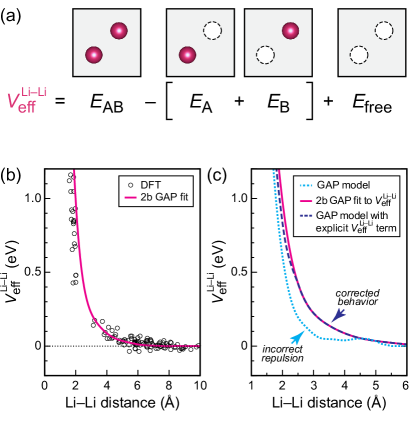
Figure 2: An effective, machine-learned potential for Li–Li interactions. (a) Schematic illustration of how the effective potential can be obtained from sets of DFT computations with atoms A and B either present or absent (Eq. 9). (b) Results of this evaluation for a range of structures with different A–B distances, showing original DFT data (circles) and a two-body (2b) GAP model that has been fitted to these data (magenta line). (c) Potential-energy scan for two Li atoms in vacuum, as a function of their interatomic distance. The dotted, light blue line shows the result of a direct GAP fit (not including the effective potential)—this underestimates the repulsion at around 3 Å, and therefore led to spurious Li–Li correlations in preliminary simulations (cf. Fig. 6 below). Including $V_{\rm eff}^{\rm Li-Li}$ in the full model (dashed, navy line) alleviates this problem.

We performed sets of such DFT computations, taking care to sample various Li–Li distances, both the strong repulsion at around 2 Å of separation and the longer-range behavior beyond 3 Å. We then fitted a 2-body GAP model to the combined data (Fig. 2b). Note that these two datasets were performed using CASTEP and VASP, respectively. This does not lead to an inconsistency since only energy differences are used here, and the absolute energy data do not enter this fit.

We stress the simplified nature of this potential: it is fitted using a two-body descriptor only, that is, it depends only on the distance between two Li atoms. Its cutoff is 9 Å, significantly longer than typically used values for short-range GAPs.

This effective potential is subtracted from the input data that enter the differential fit (Eq.  10), and subsequently it is added back to give the final, corrected result. We illustrate the need for this procedure in Fig. 2c. There, we have performed a simple diagnostic test by computing the interaction energy of two free Li atoms. An initial version of the GAP model (not including $V_{\rm eff}^{\rm Li-Li}$; dotted, light blue line) significantly underestimates the repulsion at 2–3 Å separation. In consequence, running GAP-driven MD simulations with this preliminary model led to an incorrect behavior in the Li–Li radial distribution function—that is, to an unphysical Li–Li attraction at distances at up to 4 Å. By including $V_{\rm eff}^{\rm Li-Li}$ in the full GAP model, the physical behavior is correctly recovered (dashed, navy line).

The final expression for the energy in our combined GAP model hence reads

$$E_{\rm GAP}({\rm LiC}_{x})= \,E_{\rm GAP}({\rm C}_{x})+E_{\rm DFT}({\rm Li})$$

$$+V_{\rm eff}^{\rm Li-Li}+\Delta E_{\rm GAP};$$ (10)

that is, we approximate the intercalation energy as

$$\Delta E_{\rm DFT}\approx V_{\rm eff}^{\rm Li-Li}+\Delta E_{\rm GAP}.$$ (11)

We note the analogy of the above to how molecular solids and liquids are treated using the molecular many-body expansion. Bartok2013a Beyond this particular system, we believe that such approaches will be of more general interest for those ubiquitous scenarios where relatively weak interactions need to be treated in ML-based materials simulations.

Table 1: Key parameters for the GAP models created in this work (as outlined in Fig. 1): we first fit an effective Li–Li two-body potential (Sec. II.4; parameters given in italics), and then fit a combined model for $\Delta E$ to data from which $V_{\rm eff}^{\rm Li-Li}$ has been subtracted. The notation follows the definitions in the text. $r_{\Delta}$ is a transition width for SOAP;Bartók et al. (2013) $\xi$ denotes the dimensionality of the descriptor (i.e., its number of components), and $\theta$ and $\sigma_{\rm at}$ control the smoothness of the respective kernels.

		$\Delta E$ model
		2-body	2-body	3-body	SOAP
	$V_{\rm eff}^{\rm Li-Li}$	Li–Li	Li–C	C–Li–C	Li–C
$r_{\rm cut}$ (Å)	9.0	2.5	5.5	3.5	4.5
$r_{\Delta}$ (Å)					0.5
$\xi$	1	1	1	3	606
$\delta^{(d)}$	1	10	1	0.1	0.1
$\theta$	2.2	0.8	0.8	1.2
$\sigma_{\rm at}$ (Å)					0.5
$N_{t}$ (total)	32	12	20	200	3500

III Computational details

III.1 Training database and model fitting

Initial training data were generated by randomly placing Li atoms in slightly (randomly) distorted graphite (24 atoms/cell), graphene (24 atoms/cell), and amorphous carbon (64 atoms/cell) structures (maximum Li concentration 10 atomic %). The latter were generated by quenching from the melt at different densities following Ref. 40 and using the GAP model introduced there. Single-point DFT computations were performed for all these structures: as we need the energy and force differences for fitting, reference computations for the Li-free structures were also required. To save computational time, one single Li-free structure can be used to generate several structures with one or several Li atoms present.

In most cases, we enforced a minimum Li–C distance of 1.5 Å in the training data (“hard-sphere constraint”); to accurately describe high-energy structures, we included a small amount of data where the minimum distance was lower, down to 0.70 Å. We attempted to sample configuration space widely; however, structures in which unphysically high energies ($>20$ eV/Li) or forces ($>80$ eV Å^-1) occurred were excluded (after testing several limits). The final training set contains 561 graphite, 192 graphene, and 1664 amorphous configurations.

Based on these training data, the GAP was fitted in an iterative fashion. We started by a model that only contains a two-body descriptor for Li–C interactions, and chose the parameters so as to strike a compromise between accuracy and simplicity (that is, achieving reasonable values for $r_{\rm cut}$ and $N_{t}$). Once these were optimized, the next descriptor was added (Table 1); this process was repeated until the introduction of new descriptors led to no further improvements. The potential parameter files and DFT reference database are available as described in the Data Access Statement at the end of this paper; the GAP prediction and training codes are available at http://www.libatoms.org.

III.2 DFT computations

Reference DFT computations, both for the fitting of the potential and its validation, were carried out in the local-density approximation (LDA), which had been used for the initial carbon potential due to its conceptual simplicity and its satisfactory description of the graphite interlayer distance.Deringer and Csányi (2017) In future work, it will likely be beneficial to explore the effect of advanced dispersion-correction methods such as many-body dispersion corrections,Gobre2013 but this does not affect the questions and concepts under study in this work. It is further known that the description of Li intercalation in graphite can be further improved by higher-level DFT and by Quantum Monte Carlo (QMC) methods. Ganesh et al. (2014) These are not the target here, however, due to their much higher computational cost, and since the fitting procedure is independent of the underlying DFT methodology. With more computational power available, it should be possible to fit to these quantum-mechanical methods in the future.

Single-point energy and force computations were carried out using CASTEP,Clark et al. (2005) following protocols in our previous work. Deringer and Csányi (2017) Reciprocal space was sampled on meshes with a maximum spacing of 0.03 Å^-1. The halting criterion for SCF iterations was $\Delta E<10^{-8}$ eV. Pseudopotentials were generated on-the-fly, with a plane-wave energy cutoff of 650 eV, and a correction for finite-basis errors was employed. Francis and Payne (1990)

To obtain reference data for dynamical properties of interest, viz. radial and bond-angle distributions as well as vibrational densities of states, additional DFT-based MD simulations were performed using the Vienna Ab initio Simulation Package (VASP),Kresse and Hafner (1993); Kresse and Furthmüller (1996); Kresse and Joubert (1999) the projector augmented-wave method, Blöchl (1994) and the LDA. In these simulations, the Brillouin zone was sampled at the $\Gamma$ point, which is standard practice for obtaining long MD trajectories. The plane-wave energy cutoff was 500 eV. The temperature was set to 1,000 K and controlled by a Nosé–Hoover thermostat. MD simulations were performed for 75 ps with a time step of 1 fs; the last 50 ps of the trajectories were sampled for analysis. The same or similar settings were chosen for GAP-driven MD simulations wherever possible.

IV Results and discussion

IV.1 Locality and target accuracy

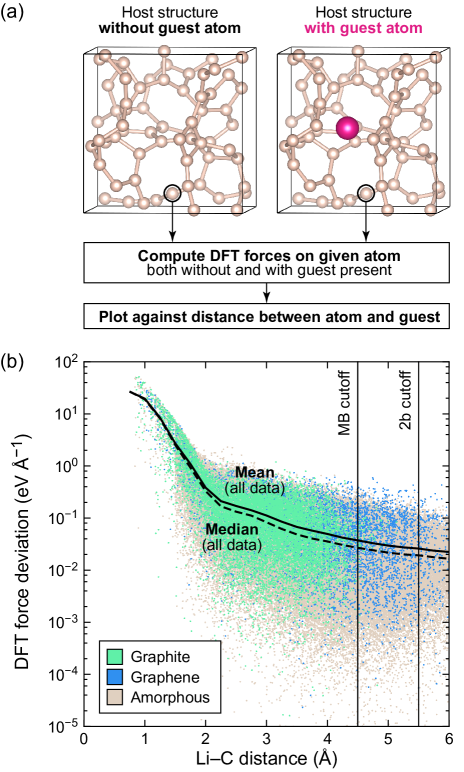
Figure 3: Locality tests for guest atoms in host structures: quantifying the maximum possible accuracy for a finite-range interatomic potential. (a) Sketch of the procedure using an exemplary amorphous carbon structure. (b) Results for a large database of graphite (green), graphene (blue), and amorphous carbon (gray) structures, with and without a single Li atom inserted in each. The mean (solid line) and median (dashed line) are collected with a binning interval of 0.25 Å.

Our potential is fitted with the assumption of locality: interactions beyond a given cutoff radius are not part of the model, and therefore a natural bound is placed on how accurate any finite-range potential can be. We have previously demonstrated how locality can be assessed for crystalline and amorphous compounds: by defining a fixed sphere around an atom in a structure, perturbing all atoms outside this sphere, and measuring the forces on the central atom as a function of sphere size. Bartók et al. (2010); Deringer and Csányi (2017) Here, we are interested in the force differences due to Li insertion, and therefore have an easier way of quantifying locality: we inspect the force components on each carbon atom in a structure with and without a single Li atom intercalated (Fig. 3a), and plot the difference (for each of the three Cartesian force components individually) as a function of how far this particular atom is away from the intercalated Li.

To make the interpretation of the data easier, we collect them with a binning interval of 0.25 Å and calculate the arithmetic mean and median values for each bin (solid and dashed lines in Fig. 3b); as their behavior is qualitatively similar, we focus on the mean in the following. The trends with Li–C distance reveal two distinct regimes: up to 2 Å, the mean deviation (which we take to indicate the expected force error of the potential) drops steeply but remains very high, as this is the region of strong Li–C interactions, not of typical cutoff radii. From 2 Å onwards, the mean still declines, indicating a remaining degree of nonlocality in the system, which would require a potential with a cutoff of $>6$ Å. However, this value must be chosen as a compromise: too large cutoffs will drastically increase the amount of required DFT reference data and also the complexity of the GAP (making it more computationally expensive in runtime). The cutoffs we use are indicated by a vertical line: note that the two-body (pairwise) descriptor extends wider than the many-body (SOAP) descriptor, and we only expect the potential to reach the accuracy relating to the latter.

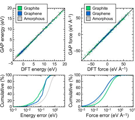
Figure 4: Top: Numerical validation of the GAP, using energies (left) and the Cartesian components of forces on atoms (right), as compared to DFT reference data. Bottom: Cumulative distributions for Li insertion energy errors per atom and force component errors, respectively. A point on these lines means that $y$ percent of the data exhibit an error of $x$ or less: the further left, the lower the error; the higher up, the higher the confidence.

This locality analysis, performed for the three different types of configurations individually (Fig. 3b), reveals similar trends but a different spatial extent: this simply mirrors the size of the supercells used, which are smallest for graphite (green) and largest for amorphous carbon (gray). Inspecting the mean as in Fig. 3b, but now for each set and at around 4.0 Å, we find deviations of 0.10, 0.08, and 0.05 eV Å^-1 for graphene, graphite, and amorphous configurations, respectively. Hence, intercalation in graphitic structures shows slightly higher nonlocality; this is qualitatively consistent with previous findings for different forms of elemental carbon. Deringer and Csányi (2017)

IV.2 Numerical errors

The most straightforward test for the quality of the GAP (or any ML potential) is computing energies and forces for the DFT database and comparing them point-by-point to the reference values. In the present work, we are studying an intercalation system, and since the host framework can be sufficiently described by the initial pure-carbon potential (Sec. II.B), we will here focus on the numerical errors for Li intercalation energies. We will show throughout this paper that, even in the presence of a notable residual numerical error, our potential can predict physical properties correctly.

The resulting energy (per atom) and force scatterplots are presented in Fig. 4. Although the overall correlation appears to be satisfactory, the numerical errors for the Li intercalation energy are notable: the root-mean-square (mean absolute) energy errors are 0.37 (0.29) eV/at., respectively. We re-iterate that the DFT reference database includes a large number of amorphous configurations on purpose, as well as small Li–C distances (below 1 Å in a few cases; Fig. 3b). Indeed, for the amorphous subset of DFT data, the errors are highest (RMSE of 0.43 eV/at.), whereas for the graphite and graphene subsets they are lower (0.17 and 0.19 eV/at., respectively). For the present proof-of-concept study, it was our target to sample configuration space as broadly as possible, and to show that this set of training data suffices to recover the dynamics of Li atoms in graphitic-like frameworks. In future work, it may be interesting to fit to larger databases sampled from GAP-driven MD trajectories, and thus to sample a more constrained region of configuration space, in turn achieving higher numerical accuracy.

Importantly, despite the notable residual energy error, the present version of the GAP performs very well in reproducing dynamical properties in MD trajectories, as will be shown in Sec. IV.C below. We believe that this is partly due to a satisfactory reconstruction of the interatomic forces. The root-mean-square and mean absolute errors are 0.25 and 0.12 eV Å^-1 (Fig. 4b), respectively, and are significantly better than those for our initial carbon GAP (on the order of 1 eV Å^-1; Ref. 40). This can be compared to a mean absolute error of 0.06 eV Å^-1 for a state-of-the-art ML model tested on distorted crystal structures of Al,Botu and Ramprasad (2015) or to an RMSE of 0.46 eV Å^-1 for a highly succcessful neural-network potential for amorphous GeTe.Sosso et al. (2012) Naturally, the more distorted and diverse the local atomic environments, the larger the overall error will become. We stress that even with a residual force error, the previous potential had afforded very accurate predictions of structural, mechanical, and surface properties.Deringer and Csányi (2017) Indeed, looking at numerical errors alone appears to be not enough when benchmarking effective potentials for amorphous materials.

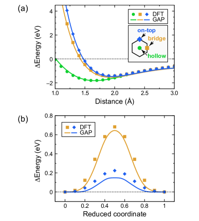
Figure 5: Tests of the GAP (line) versus DFT (symbols) for two basic atomistic processes: the adsorption of an Li atom on high-symmetry sites of a graphene sheet (a), and the diffusion of an Li atom between two potential-minimum sites in graphite across two high-symmetry pathways (b).

As less comprehensive but more demonstrative tests, we next computed characteristic energy profiles for the most fundamental atomic-scale mechanisms in the Li–graphite system. We traced the energy profiles of an Li atom that is adsorbed on different high-symmetry sites of a graphene sheet, and of an Li atom that diffuses through pristine graphite, performing DFT computations for reference that are not included in the fit. All three high-symmetry adsorption sites are correctly captured by the GAP (Fig. 5a), including the clear preference for the hollow site, and the behavior both at short and long distances is correctly reproduced. The two diffusion pathways in graphite are also qualitatively correctly described (Fig. 5b), albeit a deviation from the DFT data is visible; as the overall energy differences involved are smaller, the relative error is slightly more pronounced. Still, this result is satisfactory as the GAP has to reconstruct the pathway based on the training data, which do not include the precise pathway itself. It is also noted that our numerical tests are highly simplified, by assuming a perfectly ordered graphite structure; in contrast, experimentally determined diffusion activation energies of Li in different carbonaceous materials span a wide range (see, e.g., Ref. 73).

IV.3 Molecular-dynamics simulations

The most important question, however—and one that is very difficult to describe with DFT—, is the description of diffusion through molecular-dynamics (MD) simulations. Recall that for highly ordered systems, diffusivities have been extracted from NEB simulations of individual jumps, Persson et al. (2010); Islam and Fisher (2014) using the Arrhenius equation, but this is not easily possible in disordered and amorphous structures as there is a plethora of different pathways to be considered, each with their own associated barrier. A seminal study described DFT-driven MD simulations of Li intercalation in carbon nanotubes, but also pointed out the limitations of the method.Meunier et al. (2002) This underlines why new and flexible interatomic potentials are needed for such applications.

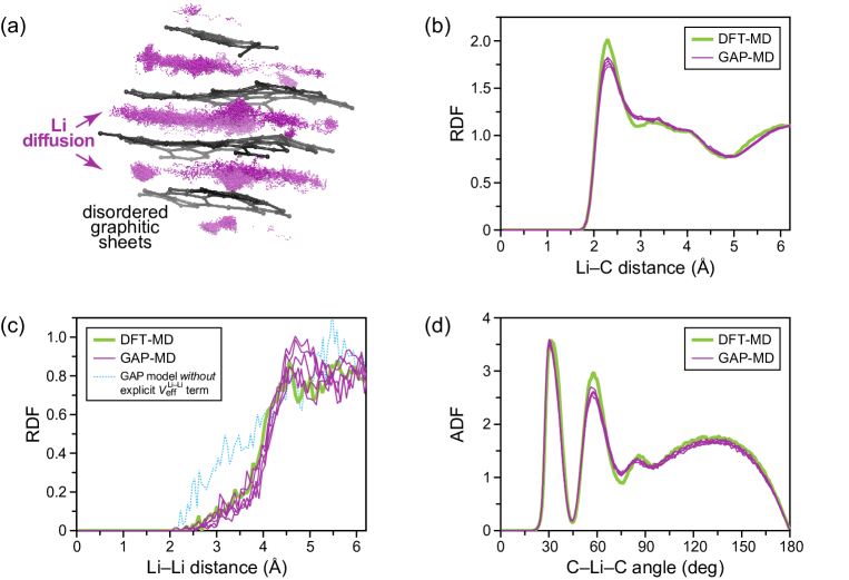
Figure 6: Molecular-dynamics simulations of Li diffusion in a graphite-like framework at 1,000 K. Results of GAP-MD have been structurally benchmarked against DFT-MD data. (a) Exemplary GAP-MD trajectory, visualized by plotting coordinates of Li atoms at equally spaced time intervals as purple dots, whereas the carbon framework is shown at a single time step to ease visibility. (b) Radial distribution function (RDF) analysis for Li–C contacts in this DFT-MD trajectory (green) and for five separate GAP-MD trajectories computed in the same structure (purple). (c) Same for the Li–Li RDF. One exemplary dataset is shown for a GAP-MD simulation using a potential without an effective Li–Li potential included (Sec. II.4), and this clearly evidences overestimated Li–Li interactions at distances up to 4 Å (dashed light blue line). (d) Same for the angular distribution function (ADF), determined for all C–Li–C angles with a maximum bond length of 3.0 Å.

To directly assess the performance of our GAP, we performed MD simulations of an ensemble of four Li atoms in a disordered graphite-like structure (Fig. 6a); the latter consists of predominantly sp²-bonded sheets, reminiscent of graphite but with several defects (five- and seven-membered rings, as well as a covalently bonded link between two sheets). This provides us with a suitable test system which allows us to probe the interaction of Li atoms with a diverse range of environments; the simulation cell is small enough to be amenable to DFT computations, and so we can generate benchmark results for properties of interest. While we have only been able to obtain a single DFT-MD trajectory, we performed several parallel GAP-MD runs due to the much lower computational cost; each of these started from the same structure but with different initial velocities.

To probe the interaction of Li atoms both with the carbon framework and with one another, we inspect the radial distribution function (RDF) and angular distribution function (ADF) curves (Fig. 6b–d). The agreement for both is highly satisfactory, especially given a certain inherent scatter in the GAP data (which is not a consequence of the method but of the system size) and the fact that our model has only been trained on small idealized graphite and graphene configurations as well as on fully amorphous structures.

The Li–C RDF (Fig. 6b) is the most direct structural “fingerprint” of Li intercalation: it shows a maximum at around 2.3 Å both in DFT- and GAP-driven MD. Small differences remain, in that the GAP-derived peak is slightly less pronounced; this is concomitant with a lowering of the average coordination number, obtained by integrating over the first RDF peak up to 2.6 Å, from 7.3 (DFT) to 6.9 (GAP). The Li–Li RDF (Fig. 6c), likewise, is an important quality criterion: it is where we observed the need for including an effective Li–Li potential in the final GAP model (Sec. II.4), and the latter correctly reproduces the very low likelihood of finding two Li atoms within 4 Å of one another. By contrast, the erroneous behavior already discussed above is clearly seen at the hand of one exemplary GAP-MD trajectory driven by a model without this effective potential (dashed, light blue line). In addition to these RDF analyses, the ADF in Fig. 6d is a more complex structural indicator, and is also very satisfactorily reproduced by GAP-MD.

We assume that the remaining small differences, in part, may be due to likewise small differences in the underlying DFT methods: different implementations and pseudopotentials are used for generating the GAP reference data and the DFT-MD trajectory. Still, the GAP reproduces all general structural features.

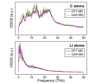
Figure 7: Vibrational densities of states (VDOS), plotted for individual MD trajectories as in Fig. 6b–c, and separately for the host structure (top) and guest atoms (bottom).

As a final means of validation, we extract from the trajectories the vibrational densities of states (VDOS), using the velocity–velocity autocorrelation function. This provides information about the atomic motion in the simulations and a link between local structure and diffusion dynamics. We inspect the VDOS individually, both for the host framework and the Li atoms, in Fig. 7. There is good agreement between DFT and GAP data, and the general features of the VDOS are well reproduced by our model. This is particularly so in the higher-frequency range ($>15$ THz), which relates mostly to interatomic interactions (such as bond-stretching vibrations). At lower frequencies, we observe small discrepancies, while the general trends are preserved. This frequency range is commonly associated with the diffusion process, and so the above can be understood considering the short run-time of the calculation and especially the small size of the systems (again, both are due to the inherent computational and scaling limitations of the DFT benchmark, and do not change the principal validity of our tests).

V Conclusions

Machine-learning-based interatomic potentials for guest atoms in host structures can be created by fitting to the energy and force differences which they induce. We exemplified this for Li intercalation in graphitic and disordered carbon structures, using the GAP framework to construct an interatomic potential model. Notwithstanding notable remaining numerical energy errors, reaching up to $\approx 0.4$ eV/atom for Li insertion, the potential shows satisfactory force accuracy and good transferability, and it can correctly describe the structural and vibrational properties of Li diffusion in a carbonaceous framework during high-temperature molecular-dynamics simulations. The approach is expected to be more general and can likely be applied to other classes of ML-based potentials. In the long run, this promises to establish difference-based ML potentials as a useful simulation method for electrochemistry and other technologically relevant applications.

Supplementary Material

Potential parameter files are provided as Supplementary Material.