Leading Digits of Mersenne Numbers

Abstract.

It has long been known that sequences such as the powers of $2$ and the factorials satisfy Benford’s Law; that is, leading digits in these sequences occur with frequencies given by $P(d)=\log_{10}(1+1/d)$, $d=1,2,\dots,9$. In this paper, we consider the leading digits of the Mersenne numbers $M_{n}=2^{p_{n}}-1$, where $p_{n}$ is the $n$-th prime. In light of known irregularities in the distribution of primes, one might expect that the leading digit sequence of $\{M_{n}\}$ has worse distribution properties than “smooth” sequences with similar rates of growth, such as $\{2^{n\log n}\}$. Surprisingly, the opposite seems to be the true; indeed, we present data, based on the first billion terms of the sequence $\{M_{n}\}$, showing that leading digits of Mersenne numbers behave in many respects more regularly than those in the above smooth sequences. We state several conjectures to this effect, and we provide an heuristic explanation for the observed phenomena based on classic models for the distribution of primes.

1. Introduction

1.1. Benford’s Law

If the leading digits (in base $10$) of the sequence $2$, $4$, $8$, $16$, $32$, $64$, $128$, $256$, $512$, $1024$, … of powers of $2$ are tabulated, one finds that the digit $1$ occurs around $30.1\%$ of the time, the digit $2$ occurs around $17.6\%$ of the time, while the digit $9$ occurs only around $4.6\%$ of the time. This is an instance of Benford’s Law, an empirical “law” that says that leading digits in many real-world and mathematical data sets tend to follow the Benford distribution, depicted in Figure 1, and given by

(1.1) $$P(d)=\log_{10}\left(1+\frac{1}{d}\right),\quad d=1,2,\dots,9.$$

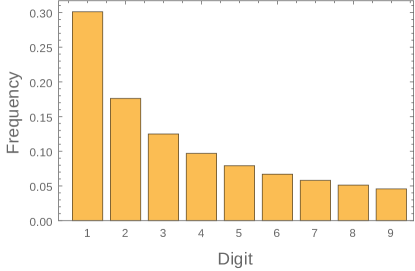
Figure 1. The Benford distribution, $P(d)=\log_{10}(1+1/d)$.

The peculiar first-digit distribution given by (1.1) is named after Frank Benford [6], who in 1938 compiled extensive empirical evidence for the ubiquity of this distribution across a wide range of real-life data sets, though it had been observed some fifty years earlier by the astronomer Simon Newcomb [31]. In recent decades, Benford’s Law has received renewed interest, in part because of its applications as a tool in fraud detection. For general background on Benford’s Law and its applications we refer to the articles by Hill [18] and Raimi [33], the in-depth survey by Berger and Hill [7], and the recent books by Berger and Hill [8], Miller [28], and Nigrini [32]. Additional references can be found in the online bibliographies [5], [9], and [20].

1.2. Benford’s Law in mathematics

From a mathematical point of view, Benford’s Law is closely connected with the theory of uniform distribution modulo $1$ [22]. In 1977 Diaconis [14] used this connection to prove rigorously that Benford’s Law holds for a class of exponentially growing sequences which includes the powers of $2$ and the sequence of factorials. That is, each of these sequences $\{a_{n}\}$ satisfies

(1.2) $$\lim_{N\to\infty}\frac{1}{N}\#\left\{n\leq N:\text{$a_{n}$ has leading digit $d$}\right\}=\log_{10}\left(1+\frac{1}{d}\right),\quad d=1,2,\dots,9.$$

Table 1 illustrates this result for the sequence of powers of $2$. The agreement between actual leading digit counts and the expected counts based on the Benford frequencies (1.1) is uncannily good: The Benford predictions are within $\pm 10$ of the actual counts among the first billion terms of the sequence.

Digit	Count	Benford Prediction	Error
1	301029995	301029995.66	-0.66
2	176091267	176091259.06	7.94
3	124938729	124938736.61	-7.61
4	96910014	96910013.01	0.99
5	79181253	79181246.05	6.95
6	66946788	66946789.63	-1.63
7	57991941	57991946.98	-5.98
8	51152528	51152522.45	5.55
9	45757485	45757490.56	-5.56

Table 1. Actual versus predicted counts of leading digits among the first $10^{9}$ terms of the sequence $\{2^{n}\}$. The predicted counts are given by $NP(d)$, where $N=10^{9}$ is the number of terms, $d$ is the digit, and $P(d)=\log_{10}(1+1/d)$ is the Benford frequency for digit $d$, given by (1.1).

More recently, Hürliman [19] investigated Benford’s Law for a variety of classical arithmetic sequences and special numbers such as the Catalan numbers. Massé and Schneider [27] established Benford’s Law for a large class of arithmetic sequences defined by growth conditions. In particular, they showed that Benford’s Law holds for sequences of the form $\lambda n^{R(n)}e^{S(n)}$, where $\lambda>0$ and $R(n)$ and $S(n)$ are polynomials satisfying some mild conditions. Examples covered by their results include the sequences $\{2^{n^{h}}\}$, where $h$ is a fixed positive integer, and $\{n^{n^{\alpha}}\}$, where $\alpha>0$.

Table 2 gives a numerical illustration of these results, based on leading digit data for the first $10^{9}$ terms of the sequences $\{2^{n^{2}}\}$, $\{2^{n\log n}\}$, and $\{n^{n}\}$. In all three cases, the deviation between the predicted and actual counts of leading digits is in the order of $10^{4}$. While not nearly as small as the errors for the sequence $\{2^{n}\}$, these deviations are comparable to the squareroot type deviation one would expect for a random sequence.

Digit	Benford Prediction	$\{2^{n^{2}}\}$	$\{2^{n\log n}\}$	$\{n^{n}\}$
1	301029995.66	2954.34	16567.34	6820.34
2	176091259.06	-6673.06	-11543.06	-10500.06
3	124938736.61	121.39	16785.39	-17051.61
4	96910013.01	-59.01	3205.99	-4763.01
5	79181246.05	7.95	-16409.05	20660.95
6	66946789.63	8897.37	6000.37	-3421.63
7	57991946.98	-3733.98	-1566.98	21179.02
8	51152522.45	236.55	-9687.45	-6807.45
9	45757490.56	-1751.56	-3352.56	-6116.56

Table 2. Deviations from predicted counts for leading digits among the first $10^{9}$ terms of the sequences $\{2^{n^{2}}\}$, $\{2^{n\log n}\}$, $\{n^{n}\}$.

1.3. Limitations of Benford’s Law

Sequences of polynomial or slower rate of growth such as the sequence of squares do not satisfy Benford’s Law in the above asymptotic density sense, though in many cases Benford’s Law can be shown to hold in some weaker form, for example, with the natural asymptotic density replaced by other notions of density; see Massé and Schneider [25] for a survey.

The failure of Benford’s Law for sequences of polynomial growth is due to the fact that the leading digits of such sequences stay constant over long enough intervals to prevent the asymptotic relation (1.2) from taking hold. For example, $n^{2}$ has leading digit $1$ whenever $n$ falls into an interval of the form $[10^{k},\sqrt{2}\cdot 10^{k})$, $k=1,2,\dots$. If (1.2) were to hold, then only a fraction $\log_{10}2\approx 0.301$ of these terms would have leading digit $1$.

In recent work [11] we exhibited another limitation to Benford’s Law for arithmetic sequences: Namely, exponentially growing sequences such as those in Table 2 tend to have very poor local Benford distribution properties, even though, from a global point of view, they provide an excellent match to Benford’s Law. For example, for the sequence $\{2^{n^{h}}\}$, where $h$ is a positive integer, $k$-tuples of leading digits of consecutive terms in the sequence do behave “independently” when $k\leq h$, but not when $k>h$.

1.4. Benford’s Law for arithmetic sequences

The current state of knowledge on the validity of Benford’s Law for “smooth” arithmetic sequences can be summarized as follows:

• Sequences such as the squares that grow at linear or polynomial rate. Benford’s Law does not hold in the usual asymptotic density sense, though it may hold with respect to other density notions such as analytic or logarithmic densities [25].

• Sequences such as $\{2^{n}\}$, $\{2^{n^{2}}\}$, or $\{n^{n}\}$ that grow at faster than polynomial rate, but whose logarithms grow at polynomial rate. Large classes of such sequences have been shown to satisfy Benford’s Law [27]. On the other hand, as shown in [11], such sequences tend to have poor local distribution properties, with the quality of the local fit to Benford’s Law being closely tied to the rate of growth of the sequence: Faster growing sequences generally are better behaved at the local level with respect to Benford’s Law.

• Sequences whose logarithms grow at faster than polynomial rate. Extrapolating from the results for the case of polynomial growth, one may expect such sequences to generally satisfy Benford’s Law, both at the global and the local level, in the sense that the associated leading digit sequence behaves like a sequence of independent Benford-distributed random variables. This can indeed be shown to be the case for “almost all” doubly exponential sequences [11], though proofs of Benford’s Law for specific sequences of doubly exponential growth such as $\{2^{2^{n}}\}$ remain elusive; see the remark at the end of [27].

1.5. Sequences involving prime numbers

The above-mentioned results focus on the leading digit behavior of “smooth” sequences, i.e., sequences of the form $\{f(n)\}$, where $f(x)$ is some well-behaved function of $x$. One can ask similar questions about sequences that are defined in terms of prime numbers. The sequence of prime numbers $\{p_{n}\}$ itself does not satisfy Benford’s Law for the same reason that polynomial sequences do not satisfy this law: Since $p_{n}\sim n\log n$ as $n\to\infty$ (see, for example, Theorem 4.1 in [1]), the rate of growth of $\{p_{n}\}$ is too slow for the asymptotic relation (1.2) to take hold. However, a number of authors have shown that the primes satisfy various weaker forms of this law; see Whitney [37], Schatte [34], Cohen and Katz [13], Fuchs and Letta [16], Luque and Lacasa [23], Eliahou et al. [15], and Massé and Schneider [25].

In light of the above heuristic, it is reasonable to expect that Benford’s Law holds for sufficiently fast growing sequences defined in terms of prime numbers. Massé and Schneider [26] showed that this is indeed the case for the sequence $\{P_{n}\}$ of primorial numbers defined by $P_{n}=\prod_{k=1}^{n}p_{k}$.

1.6. The Mersenne numbers

In this paper we consider another classic sequence involving prime numbers, the Mersenne numbers, defined as

(1.3) $$M_{n}=2^{p_{n}}-1.$$

The first twenty terms of this sequence are given in Table 3.

$n$	$p_{n}$	$M_{n}=2^{p_{n}}-1$
1	2	3
2	3	7
3	5	31
4	7	127
5	11	2047
6	13	8191
7	17	131071
8	19	524287
9	23	8388607
10	29	536870911

$n$	$p_{n}$	$M_{n}=2^{p_{n}}-1$
11	31	2147483647
12	37	137438953471
13	41	2199023255551
14	43	8796093022207
15	47	140737488355327
16	53	9007199254740991
17	59	576460752303423487
18	61	2305843009213693951
19	67	147573952589676412927
20	71	2361183241434822606847

Table 3. The first $20$ Mersenne numbers, $M_{n}=2^{p_{n}}-1$.

Since $p_{n}\sim n\log n$, the sequence $\{M_{n}\}$ has a rate of growth between that of the sequences $\{2^{n}\}$ and $\{2^{n^{2}}\}$, and very similar to that of the sequence $\{2^{n\log n}\}$. In terms of the above hierarchy, it is a sequence of type (II). Thus, one might expect the sequence $\{M_{n}\}$ to have excellent global, but poor local distribution properties with respect to Benford’s Law.

From a global point of view, the behavior is indeed as expected. We show that the sequence $\{M_{n}\}$ satisfies Benford’s Law and we provide numerical evidence suggesting that the quality of the fit is comparable to that of other sequences of similar rate of growth.

On the other hand, the local distribution of leading digits of $\{M_{n}\}$ is completely different from that of other sequences of type (II), and more like that of sequences of type (III). An illustration of these differences is given in Figure 2, which shows the distribution of “waiting times” between successive occurrences of $1$ as leading digit for the sequences $\{M_{n}\}$, $\{2^{n}\}$, $\{2^{n\log n}\}$, and $\{2^{n^{2}}\}$. Only the Mersenne sequence, $\{M_{n}\}$, exhibits the geometric waiting time distribution that one would expect for a random sequence of Benford-distributed digits. The other three sequences have distinctly different waiting time distributions.

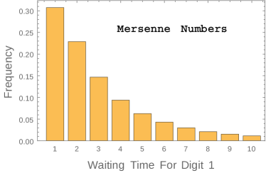
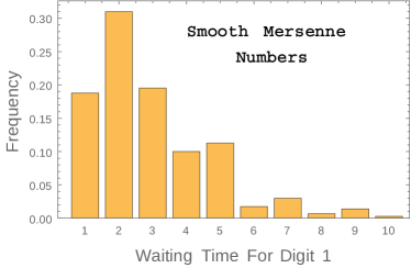
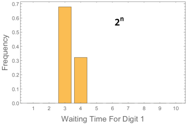
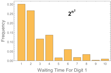
Figure 2. The distribution of “waiting times” between occurrences of leading digit $1$ for the sequence of Mersenne numbers $M_{n}=2^{p_{n}}-1$ (top left chart), and for three “smooth” sequences with similar rates of growth: $\{2^{n\log n}\}$ (top right), $\{2^{n}\}$ (bottom left), and $\{2^{n^{2}}\}$ (bottom right). Of these four sequences only the Mersenne sequence exhibits a geometric waiting time distribution.

This surprising discrepancy between the local Benford distribution properties of the sequence $\{M_{n}\}$ and similar “smooth” sequences is the main finding of this paper. We conjecture that, in contrast to smooth sequences such as those in Tables 1 and 2, the sequence of leading digits of $\{M_{n}\}$ behaves like a sequence of independent Benford-distributed random variables. We provide numerical evidence in support of this conclusion, and we give an heuristic explanation for the apparent discrepancy in the behaviors of $\{M_{n}\}$ and similar smooth sequences.

1.7. Outline of paper

The remainder of this paper is organized as follows: In Section 2 we state our main conjectures and results. In Section 3 we describe the numerical data on which these conjectures are based and the approach we have taken to generate the data. In Section 4 we show that $\{M_{n}\}$ satisfies Benford’s Law, and we provide numerical data on the quality of the fit. In Section 5 we present experimental data supporting our conjectures on the local distribution of leading digits of $\{M_{n}\}$. In Section 6 we show that smooth sequences with similar rates of growth do not satisfy these conjectures. Section 7 contains a summary of our findings, along with some remarks and open questions.

2. Summary of Results and Conjectures

2.1. Notations and definitions

Given a positive real number $x$, we denote by $D(x)$ the leading (i.e., most significant) digit of $x$ in base $10$. More precisely, we define $D(x)$ by

(2.1) $$D(x)=d\Longleftrightarrow d\cdot 10^{k}\leq x<(d+1)10^{k}\quad\text{for some $k\in\mathbb{Z}$}$$

for $d\in\{1,2,\dots,9\}$. Note that this definition does not require $x$ to be an integer; for example, we have $D(\pi)=3$ and $D(0.0314)=3$. We let $P(d)=\log_{10}(1+1/d)$ denote the Benford frequency for digit $d$, as defined in (1.1).

Definition 2.1 (Global Benford Distribution).

A sequence $\{a_{n}\}$ of positive real numbers is said to be Benford distributed (or, equivalently, said to satisfy Benford’s Law) if

(2.2) $$\lim_{N\to\infty}\frac{1}{N}\#\{n\leq N:D(a_{n})=d\}=P(d)\quad\text{for $d=1,2,\dots,9$.}$$

Definition 2.2 (Local Benford Distribution).

Let $k$ be a positive integer. A sequence $\{a_{n}\}$ of positive real numbers is called locally Benford distributed of order $k$ if

(2.3) $$\lim_{N\to\infty} \frac{1}{N}\#\{n\leq N:D(a_{n+i})=d_{i}\quad(i=0,1,\dots,k-1)\}$$

$$\qquad=P(d_{0})P(d_{1})\dots P(d_{k-1})\quad\text{for $d_{i}=1,\dots,9$ ($i=0,1,\dots,k-1$).}$$

Remarks 2.3.

(1) Definition 2.1 is one of several common definitions of Benford’s Law used in the literature. We chose this particular version over others in the literature because of its simplicity and intuitiveness.

(2) The case $k=1$ in (2.3) reduces to the definition (2.2) of a (global) Benford distributed sequence. It is immediate from the definition that a sequence that is locally Benford distributed of order $k$ is also locally Benford distributed of any order $k^{\prime}\leq k$. Thus, the concept of local Benford distribution of a sequence refines that of Benford distribution and establishes a hierarchy of classes of sequences with successively stronger local distribution properties.

(3) The above definitions can be extended in a natural way to other bases, and we expect that most of our results and conjectures remain valid for such generalized versions of Benford’s Law. We decided to focus on the standard case of base $10$ in order to avoid unnecessary notational complications. All of the features we expect to hold in the general case are already present in base $10$.

Given a sequence $\{a_{n}\}$ of positive real numbers and $d\in\{1,2,\dots,9\}$, we define sequences $\{n_{i}^{(d)}\}$ by

(2.4) $$\{n_{1}^{(d)}<n_{2}^{(d)}<n_{3}^{(d)}<\cdots\} =\{n\in\mathbb{N}:D(a_{n})=d\},$$

and we let

(2.5) $$w_{i}{(d)} =n_{i+1}^{(d)}-n_{i}^{(d)}.$$

In other words, the numbers $n_{i}^{(d)}$ are the successive indices $n$ at which $a_{n}$ has leading digit $d$, and the numbers $w_{i}^{(d)}$ are the “waiting times”, or gaps, between these occurrences.

If $\{a_{n}\}$ is Benford distributed, then the numbers $n_{i}^{(d)}$ occur with asymptotic frequency $P(d)$, so the average gap between these numbers is $1/P(d)$, i.e., we have

(2.6) $$\lim_{N\to\infty}\frac{1}{N}\sum_{i\leq N}w_{i}(d)=\frac{1}{P(d)}\quad\text{for $d=1,2,\dots,9$.}$$

In fact, it is not hard to see that the converse is also true. That is, (2.6) holds if and only if $\{a_{n}\}$ is Benford distributed.

In general, the average statement (2.6) is all we can say about the waiting times of a sequence that is Benford distributed. However, for sequences that are locally “well behaved” we expect more to be true: Namely, we expect the waiting times between these occurrences to have geometric distribution with mean $1/P(d)$. We thus make the following definition.

Definition 2.4 (Benford Distributed Waiting Times).

A sequence $\{a_{n}\}$ of positive real numbers is said to have Benford distributed waiting times if

(2.7) $$\lim_{N\to\infty}\frac{1}{N}\#\left\{i\leq N:w_{i}(d)=k\right\} =P(d)(1-P(d))^{k-1}$$

for $$d=1,2,\dots,9 k=1,2,\dots$$ and .

It is not hard to see that a sequence that is locally Benford distributed of any order $k$ has Benford distributed waiting times. Thus, we have the chain of implications:

Locally Benford distributed of any order $$k$$, (2.3)

$$\Downarrow$$

Benford distributed waiting times, (2.7)

$$\Downarrow$$

Average waiting time property, (2.6)

$$\Updownarrow$$

$$\text{Benford's Law, \eqref{eq:benford3}}.$$

2.2. Global distribution properties

Recall the definition of the Mersenne numbers:

$$M_{n}=2^{p_{n}}-1,$$

where $p_{n}$ denotes the $n$-th prime.

Theorem 2.5 (Benford Law for $\{M_{n}\}$).

The sequence $\{M_{n}\}$ is Benford-distributed i.e., satisfies (2.2).

This result is a consequence of a theorem of Vinogradov [36] and may be known to experts in the field, but we were unable to find a specific reference in the literature. We will supply a proof in Section 4.

In light of this result, it is natural to consider the size of the error in the Benford approximation for the frequencies of leading digits of $\{M_{n}\}$, i.e., the quantities

(2.8) $$E_{d}(N)=\#\{n\leq N:D(M_{n})=d\}-NP(d).$$

As Tables 1 and 2 show, for smooth sequences the size of this error can vary dramatically, from a logarithmic or even bounded error in the case of $\{2^{n}\}$ to the squareroot size oscillations typically associated with random sequences. Our data (see Section 4) suggests that the sequence $\{M_{n}\}$ falls into the latter class.

Conjecture 2.6 (Benford Error for $\{M_{n}\}$).

The Benford errors $E_{d}(N)$ defined by (2.8) satisfy

$$E_{d}(N)=O(N^{1/2+\epsilon})\quad\text{and}\quad E_{d}(N)\not=O(N^{1/2-\epsilon})$$

for any fixed $\epsilon>0$.

2.3. Local distribution properties

We now turn to the local distribution properties of the leading digits of $\{M_{n}\}$. We make the following conjectures.

Conjecture 2.7 (Local Benford Distribution of $\{M_{n}\}$).

The sequence $\{M_{n}\}$ is locally Benford distributed of any order $k$. That is, for any positive integer $k$, the leading digits of $k$-tuples of consecutive terms in this sequence behave like $k$ independent Benford-distributed random variables.

Conjecture 2.8 (Benford Waiting Times for $\{M_{n}\}$).

The sequence $\{M_{n}\}$ has Benford-distributed waiting times. That is, the waiting times between occurrences of leading digit $d$ behave like geometric random variables with parameter $p=P(d)$.

These conjectures are motivated by the numerical data we will present in Section 5 of this paper, and by heuristic arguments, described in Section 7 and based on classical conjectures about the local distribution of primes.

In stark contrast to the behavior of $\{M_{n}\}$ predicted by these conjectures, the following result shows that smooth sequences with similar growth rates do not satisfy the conjectures.

Theorem 2.9 (Failure of Local Benford Law for Mersenne-like Smooth Sequences).

Let $\{a_{n}\}$ be a sequence of positive real numbers such that the logarithmic differences

$$\Delta\log a_{n}=\log a_{n+1}-\log a_{n}$$

satisfy

(2.9) $$\Delta\log a_{n}\to\infty\quad(n\to\infty)$$

and

(2.10) $$\Delta\log a_{n+1}=\Delta\log a_{n}+O\left(\frac{1}{n}\right)\quad(n\to\infty).$$

Then:

• $\{a_{n}\}$ is not locally Benford distributed of order $k$ when $k\geq 2$.

• $\{a_{n}\}$ does not have Benford distributed waiting times.

The theorem applies to a large class of smooth sequences with growth rates similar to that of the Mersenne numbers. In particular, it is easy to check that conditions (2.9) and (2.10) hold for the sequences $\{n!\}$, $\{n^{n}\}$, and $\{2^{n\log n}\}$. Thus we have the following corollary.

Corollary 2.10.

The sequences $\{n!\}$, $\{n^{n}\}$, and $\{2^{n\log n}\}$ are not locally Benford distributed of order $2$ (or larger) and do not have Benford distributed waiting times.

For more general results of this type see [11].

Figure 2 illustrates the difference in the waiting time behavior between the sequence of Mersenne numbers, $\{M_{n}\}$, and the sequence of “smooth Mersenne numbers”, $\{2^{n\log n}\}$. For the sequence of Mersenne numbers the waiting time distribution resembles a geometric distribution very closely, while for its smooth analog, the waiting times seem to have an irregular distribution that is quite far from a geometric distribution.

3. Description of Data and Implementation Notes

3.1. Description of data

Our analysis is based on the leading digits of the first billion terms of the following sequences:

• Mersenne numbers. The Mersenne numbers, defined as $M_{n}=2^{p_{n}}-1$, where $p_{n}$ is the $n$-th prime, form our main object of investigation.

• Random Mersenne numbers. Random Mersenne numbers form one of our “control” sequences against which we compare the leading digit behavior of the Mersenne numbers. They are defined as $M_{n}^{*}=2^{p_{n}^{*}}-1$, where $\{p_{n}^{*}\}$ is a sequence of “random” primes obtained by declaring an integer $n\geq 3$ to be a prime with probability $1/\log n$.

• Smooth Mersenne numbers. The sequence of “smooth” Mersenne numbers, defined as $2^{n\log n}$, constitutes our second main “control” sequence for the Mersenne numbers. The smooth Mersenne numbers are essentially the numbers obtained by replacing the $n$-th prime, $p_{n}$, in the definition of $M_{n}$ by its smooth asymptotic, $n\log n$.

• Other “smooth” sequences. Additional smooth sequences we have used as points of comparisons in some of our analyses are the sequences $\{2^{n}\}$ and $\{2^{n^{2}}\}$.

3.2. Generating the leading digits

Because of the size of the numbers involved (for example, the billionth Mersenne number has more than six billion decimal digits), computing the necessary sequences of leading digits is a nontrivial task. For our primary sequence, the Mersenne numbers, we proceeded as follows:

1. Generate the prime numbers $p_{n}$, $n=1,2,\dots,10^{9}$, using an optimized version of the sieve of Eratosthenes, obtained from http://primesieve.org.

2. For each such $p_{n}$, compute $\{p_{n}\log_{10}2\}$, where $\{t\}$ denotes the fractional part of $t$, and determine the unique integer $d\in\{1,2,\dots,9\}$ such that

   $$\log_{10}d\leq\{p_{n}\log_{10}2\}<\log_{10}(d+1).$$

   This value of $d$ is the leading digit of $2^{p_{n}}$ in base $10$. To get accurate values of leading digits, we used the REAL data type from the C++ library iRRAM, http://irram.uni-trier.de, a library for error-free real arithmetic (see Müller [30]).

3. To obtain the leading digits for the Mersenne numbers $2^{p_{n}}-1$, observe that $2^{p_{n}}-1$ and $2^{p_{n}}$ have the same leading digit unless $p_{n}=2$ or $p_{n}=3$. Indeed, if $2^{m}-1$ has leading digit $d$, then $d\cdot 10^{k}\leq 2^{m}-1<(d+1)\cdot 10^{k}$ for some nonnegative integer $k$, which implies $d\cdot 10^{k}\leq 2^{m}<(d+1)\cdot 10^{k}$ unless $2^{m}=(d+1)10^{k}$. But the latter equation can only hold if $k=0$, i.e., if $2^{m}=d+1\leq 10$. Thus, except for the two terms corresponding to $p_{1}=2$ and $p_{2}=3$, the leading digit of $2^{p_{n}}$ obtained in the previous step is also the leading digit of the Mersenne number $2^{p_{n}}-1$. Adjusting for the two exceptional terms gives the leading digit sequence for the Mersenne numbers.

Leading digits of the various smooth analogs of the Mersenne numbers were generated in the same way, with the sequence of prime numbers in the first step replaced by the appropriate smooth sequence.

3.3. Generating random Mersenne numbers

Random Mersenne numbers were generated in the same way as Mersenne numbers, with the sequence of primes, $\{p_{n}\}$, replaced by a sequence of random primes, $\{p_{n}^{*}\}$, obtained as follows:

1. For each $n\geq 3$ generate a random real number $R_{n}$ in the interval $[0,1]$. As random number generator we used the uniform_real_distribution function from the C++ standard library.

2. If $R_{n}\leq 1/\log n$, declare $n$ to be a random prime.

3. Let $p_{1}^{*}<p_{2}^{*}<\cdots<p_{10^{9}}^{*}$ be the ordered sequence of the first $10^{9}$ random primes obtained.

The second step ensures that the random primes generated occur with density $1/\log n$, which is the actual density of prime numbers near $n$. Indeed, by a classic form of the prime number theorem (see, for example, Theorem 8.15 in [4]) we have

$$\#\{n\leq N:n\text{ is prime }\}=\int_{2}^{N}\frac{1}{\log x}dx+O\left(N\exp\left(-c\sqrt{\log N}\right)\right),$$

where $c$ is a positive constant.

3.4. Implementation notes

Most of the computations were carried out at the Taub node of the Illinois Campus Computing Cluster, https://campuscluster.illinois.edu/hardware/#taub, a multi-core high performance computing platform running Scientific Linux 6.1, with 96 GB of RAM. The primary data sets of leading digits were generated and analyzed with C++ programs, compiled with GNU g++ -std=c++11. Generating one billion leading digits took around 5–10 hours of CPU time. Python 3.4 was used for additional lighter weight analysis and string manipulation.

4. Global Distribution Properties

4.1. Empirical data on global distribution. Evidence for Conjecture 2.6

We begin by presenting numerical data on the frequencies of leading digits in the sequence of Mersenne numbers $M_{n}=2^{p_{n}}-1$. Table 4 shows the actual counts for leading digits among the first billion Mersenne numbers, along with the predicted counts based on the Benford frequencies (1.1). In all cases, the actual and predicted counts agree to at least three digits.

Digit	Count	Benford Prediction	Error
1	301032256	301029995.66	2260.34
2	176095018	176091259.06	3758.94
3	124946964	124938736.61	8227.39
4	96901940	96910013.01	-8073.01
5	79176717	79181246.05	-4529.05
6	66950369	66946789.63	3579.37
7	57993513	57991946.98	1566.02
8	51145193	51152522.45	-7329.45
9	45758030	45757490.56	539.44

Table 4. Actual versus predicted counts of leading digits among the first $10^{9}$ Mersenne numbers. The predicted counts are given by $NP(d)$, where $N=10^{9}$ is the number of terms, $d$ is the digit, and $P(d)=\log_{10}(1+1/d)$ is the Benford frequency for digit $d$, given by (1.1).

The errors in Table 4 appear to be roughly of the squareroot size predicted by Conjecture 2.6. For a more detailed analysis, we compare these errors to those in a random model in which the events “$M_{n}$ has leading digit $d$”, $n=1,2,\dots$, are assumed to be independent events with probability $P(d)=\log_{10}(1+1/d)$. Under this assumption, the Central Limit Theorem yields that the number of terms with leading digit $d$ among the first $N$ terms $M_{n}$ is approximately normally distributed with mean $NP(d)$ and standard deviation $\sqrt{N\cdot P(d)(1-P(d))}$. This motivates normalizing the error to a z-score, defined as

(4.1) $$z(d,N)=\frac{\#\{n\leq N:D(M_{n})=d\}-NP(d)}{\sqrt{N\cdot P(d)(1-P(d))}}.$$

Figure 3 shows the behavior of these z-scores as functions of $N$ for the digits $1$, $2$, $5$, and $9$. In all cases, the z-scores exhibit the typical random walk type behavior associated with sequences of independent Bernoulli random variables.

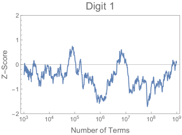
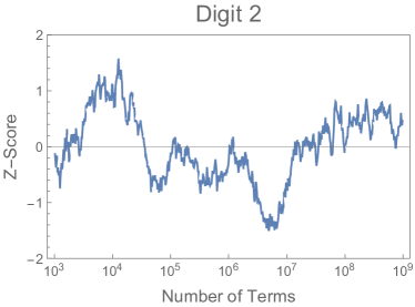
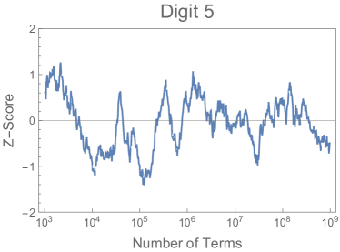
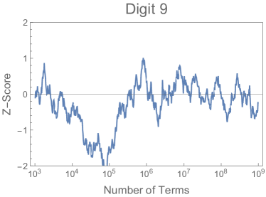
Figure 3. The behavior of the normalized errors, given by the z-scores (4.1), in the leading digit counts for Mersenne numbers for digits $1$, $2$, $5$, and $9$. In all cases, the z-scores exhibit the typical random-like behavior one would observe if the digits were to occur independently with Benford frequencies (1.1).

Additional insight is provided by the two charts of Figure 4, which show the distribution of z-scores $z(d,N)$, as $N$ runs through the geometrically spaced sample points $N_{i}=\lfloor 10^{3}\cdot 1.05^{i}\rfloor$, $i=1,2,\dots,696$. The box-whisker chart on the left shows, for each digit $d$, the median, quartiles, and extreme values of the corresponding set of z-scores. The histogram on the right displays the combined distribution of these z-scores for all digits $d$. In particular, the data shows that all z-scores sampled fall into the interval $[-3,3]$ and that most are spread out over the subinterval $[-1,1]$. In other words, within the data we have sampled the error in the Benford approximation for leading digit counts is within a factor $\pm 3$ of $\sqrt{N\cdot P(d)(1-P(d))}$, and the latter quantity represents the “typical” size of the error. This lends strong support to Conjecture 2.6, which states that the error is order $O(N^{1/2+o(1)})$, but not of smaller order of magnitude.

In fact, it may be the case that these errors, after normalizing by $\sqrt{N\cdot P(d)(1-P(d))}$, converge, in an appropriate sense (for example, in the sense of logarithmic density), to a standard normal distribution. This would represent a significant refinement of Conjecture 2.6.

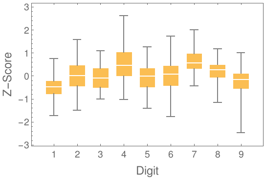
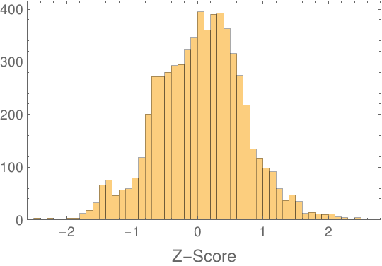
Figure 4. The distribution of the normalized errors, given by the z-scores (4.1), in the leading digit counts for Mersenne numbers. The box-whisker chart shows the distribution of z-scores $z(d,N)$ for each individual digit $d$. The histogram shows the combined distribution of these z-scores over all digits $d$.

4.2. Proof of Theorem 2.5

To conclude this section, we show that the sequence $\{M_{n}\}$ satisfies Benford’s Law. The proof is short, but it relies on two key results from the literature. The first result introduces an important tool in establishing Benford’s Law for mathematical sequences, namely the concept of uniform distribution modulo $1$.

Definition 4.1 (Uniform Distribution Modulo $1$).

A sequence of real numbers $\{u_{n}\}$ is called uniformly distributed modulo $1$ if it satisfies

(4.2) $$\lim_{N\to\infty}\frac{1}{N}\#\{n\leq N:\{u_{n}\}\leq t\}=t\quad(0\leq t\leq 1),$$

where $\{x\}$ denotes the fractional part of $x$.

The connection between uniform distribution and Benford’s Law is given in the following proposition, due to Diaconis [14, Theorem 1].

Proposition 4.2 (Diaconis).

Let $\{a_{n}\}$ be a sequence of positive real numbers. If the sequence $\{\log_{10}a_{n}\}$ is uniformly distributed modulo $1$, then $\{a_{n}\}$ satisfies Benford’s Law.

The second ingredient in the proof is the following result of Vinogradov [36] (see also Iwaniec and Kowalski [21, Theorem 21.3]).

Proposition 4.3 (Vinogradov).

Let $\alpha$ be an irrational number. Then the sequence $\{\alpha p_{n}\}$ is uniformly distributed modulo $1$.

Proof of Theorem 2.5.

Let $u_{n}=\log_{10}M_{n}$. By Proposition 4.2, to show that $\{M_{n}\}$ satisfies Benford’s Law, it suffices to show that the sequence $\{\log_{10}M_{n}\}$ is uniformly distributed modulo $1$. Now,

(4.3) $$\log_{10}M_{n}=\log_{10}(2^{p_{n}}-1)=(\log_{10}2)p_{n}+o(1)\quad(n\to\infty).$$

Since $\log_{10}2$ is irrational, Proposition 4.3 implies that the sequence $\{(\log_{10}2)p_{n}\}$ is uniformly distributed modulo $1$. To conclude that $\{\log_{10}M_{n}\}$ is also uniformly distributed modulo $1$, it suffices to observe that if $\{u_{n}\}$ is uniformly distributed modulo $1$, then any sequence $\{u_{n}^{*}\}$ satisfying $u_{n}^{*}=u_{n}+o(1)$ as $n\to\infty$ is also uniformly distributed modulo $1$. The latter claim follows immediately from the definition (4.2) of uniform distribution modulo $1$. ∎

Remark 4.4.

An interesting question is to what extent the error in the uniform distribution result of Proposition 4.3 depends on diophantine approximation properties of $\alpha$. We are not aware of any results of this type in the literature, though such error bounds could in principle be obtained from appropriate exponential sum estimates (e.g., Theorem 4.2 in Banks and Shparlinski [2]) via the Erdös-Turan inequality as in the proof of [22, Chapter 2, Theorem 3.2]. The resulting error bounds would, however, likely be quite far from being best-possible.

5. Local Distribution Properties

5.1. Empirical data on waiting times. Evidence for Conjecture 2.8

We begin by providing data in support of the waiting time conjecture, Conjecture 2.8. Figure 5 shows the distribution of waiting times between occurrences of leading digit $1$ among the first $10^{9}$ terms of the sequence of Mersenne numbers, along with the analogous distributions for three “control” sequences: “random” Mersenne numbers, $2^{p_{n}^{*}}-1$, where $\{p_{n}^{*}\}$ is a sequence of random primes (see Section 3); “smooth” Mersenne numbers, defined as $2^{n\log n}$; and the sequence $\{2^{n^{2}}\}$.

For each of these sequences, the observed frequencies for waiting times $1,2,\dots,10$ are shown along with the “theoretical” frequencies, given by

(5.1) $$P(\text{waiting time between $1$'s is $k$})=p(1-p)^{k-1},\quad k=1,2,\dots,$$

where $p=\log_{10}2$ is the Benford probability for leading digit $1$. For the Mersenne numbers and random Mersenne numbers the agreement between the predicted and actual waiting time distribution is very good. By contrast, the smooth analogs of $M_{n}$, shown in the bottom two charts of Figure 5, have a noticeably different waiting time distribution.

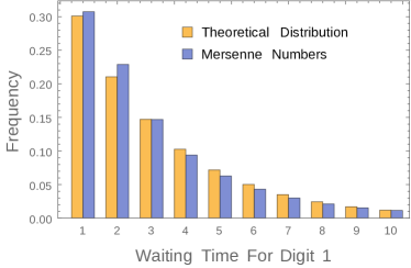
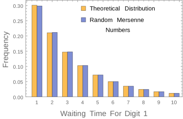
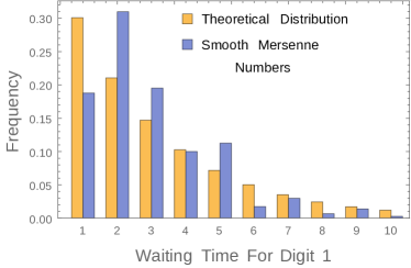
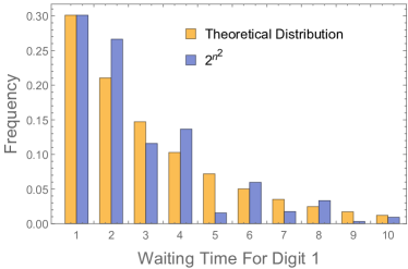
Figure 5. The distribution of “waiting times” between occurrences of leading digit $1$ among the first $10^{9}$ terms of four sequences: the Mersenne numbers $M_{n}=2^{p_{n}}-1$; “random” Mersenne numbers, $2^{p_{n}^{*}}-1$, where $p_{n}^{*}$ denote “random” primes; “smooth” Mersenne numbers, $2^{n\log n}$; and the sequence $\{2^{n^{2}}\}$. Of these four sequences only the Mersenne sequence and its random analog exhibit a geometric waiting time distribution.

For another perspective on the behavior of the waiting times between leading digits, we consider the waiting time frequencies as functions of the number of terms in the sequence. For the Mersenne sequence the results are shown in Figure 6: The observed frequencies are close to the predicted frequencies at all sample points, and the agreement improves as the number of terms increases.

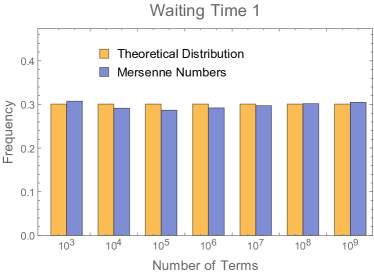
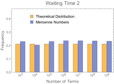
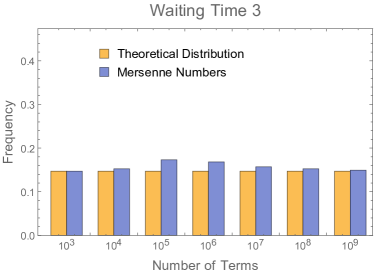
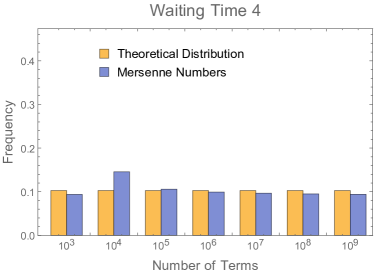
Figure 6. Frequencies of waiting time $k$ (where $k=1,2,3,4$) between occurrences of leading digit $1$ among the first $10^{i}$ Mersenne numbers ($i=3,\dots,9$), along with the theoretical frequencies given by (5.1).

Figure 7 shows the same set of waiting time frequencies for the sequence of smooth Mersenne numbers. Here the behavior is completely different from the case of Mersenne numbers. Not only do the observed frequencies differ significantly from the theoretical distribution, they also exhibit large oscillations as the number of terms increases, suggesting that a limit distribution does not exist.

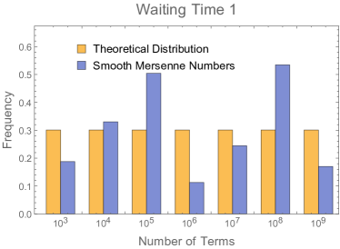
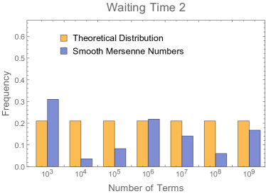
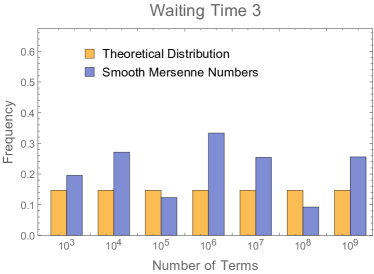
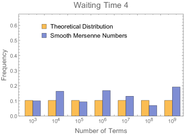
Figure 7. Frequencies of waiting time $k$ (where $k=1,2,3,4$) between occurrences of leading digit $1$ among the first $10^{i}$ smooth Mersenne numbers ($i=3,\dots,9$), along with the theoretical frequencies given by (5.1).

5.2. Empirical data on local distribution of leading digits. Evidence for Conjecture 2.7

We next consider Conjecture 2.7, which predicts that, for any fixed positive integer $k$, $k$-tuples of leading digits of consecutive terms behave like $k$ independent Benford-distribution random variables. That is, each tuple $(d_{1},\dots,d_{k})$ of leading digits is predicted to occur with asymptotic frequency

(5.2) $$P(d_{1},\dots,d_{k})=\prod_{i=1}^{k}P(d_{i})=\prod_{i=1}^{k}\log_{10}\left(1+\frac{1}{d_{i}}\right).$$

For $k=1$, (5.2) reduces to the (global) Benford distribution, which we had considered in Section 4. The case $k=2$ therefore is the first test case for local Benford distribution properties of a sequence. We have focused our numerical computations on this case as for larger $k$-values the densities become too small to yield meaningful numerical data within the computable range. However, indirect evidence that the behavior predicted by Conjecture 2.7 also holds when $k\geq 3$ is provided by our data on waiting time distributions: The frequencies for waiting time $k$ between occurrences of a given leading digit depend on the joint distribution of $(k+1)$-tuples of leading digits. Thus, the close agreement that we found between observed and predicted waiting time frequencies for the sequence of Mersenne numbers suggests that this sequence does indeed have the predicted joint distribution (5.2).

Table 5 shows the observed and predicted frequencies of four pairs $(d_{1},d_{2})$ of leading digits among the first $10^{9}$ terms of the sequences of Mersenne numbers, random Mersenne numbers, and smooth Mersenne numbers.

$(d_{1},d_{2})$	Prediction	Mersenne	Random Mersenne	Smooth Mersenne
$(1,1)$	0.09062	0.09252	0.08989	0.05748
$(1,2)$	0.05301	0.04916	0.05072	0.07228
$(2,1)$	0.05300	0.05811	0.05447	0.01503
$(2,2)$	0.03101	0.02905	0.02963	0.01863

Table 5. Actual versus predicted frequencies of selected pairs $(d_{1},d_{2})$ of leading digits among the first $10^{9}$ terms of the sequences of Mersenne numbers, random Mersenne numbers, and smooth Mersenne numbers. The predicted frequencies are those given by (5.2).

Figure 8 shows these frequencies as a function of the number of terms in the sequence. For the Mersenne and random Mersenne numbers, the frequencies indeed seem to converge to their predicted values, (5.2), thus lending support to Conjecture 2.7. On the other hand, for the smooth Mersenne numbers, the behavior is completely different: The frequencies of pairs of leading digits exhibit a distinct oscillating behavior and do not seem to converge to a limit. Moreover, they do not seem to be symmetric; for example, the pair $(1,2)$ occurs about four times as often as the pair $(2,1)$ among the first $10^{9}$ terms in the sequence.

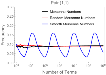
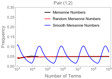
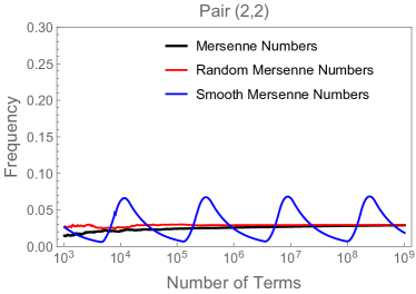
Figure 8. The distribution of pairs $(d_{1},d_{2})$ of leading digits of successive terms in the sequences of Mersenne numbers, random Mersenne numbers, and smooth Mersenne numbers. The behavior of the latter sequence is distinctly different from that of the former two sequences. For the Mersenne and random Mersenne sequences the frequencies appear to converge to the expected limit, given in the first column of Table 5, while for the smooth Mersenne numbers these frequencies exhibit an oscillating behavior.

For additional insight and support for Conjecture 2.7, we consider the variation distance between the observed and predicted pair distributions. The variation distance (or total variation distance) is a standard distance measure for probability distributions. Given discrete probability distributions $P$ and $Q$ on a (finite or countable) probability space $\Omega$, the variation distance between $P$ and $Q$ is defined as

(5.3) $$\operatorname{d_{TV}}(P,Q)=\frac{1}{2}\sum_{\omega\in\Omega}|P(\omega)-Q(\omega)|.$$

In the case $\Omega$ is the set of $k$-tuples $(d_{1},\dots,d_{k})$, $d_{i}=1,2,\dots,9$, and $P$ the predicted distribution on this set given by (5.2), this definition reduces to

(5.4) $$\operatorname{d_{TV}}(P,Q)=\frac{1}{2}\sum_{d_{1},\dots,d_{k}=1}^{9}\left|P(d_{1})\dots P(d_{k})-Q(d_{1},\dots,d_{k})\right|,$$

where $P(d)=\log_{10}(1+1/d)$ are the individual Benford frequencies for digit $d$.

Conjecture 2.7 can be restated in terms of the variation distance $\operatorname{d_{TV}}$: The conjecture is equivalent to the statement $\operatorname{d_{TV}}(Q_{N},P)\to 0$ as $N\to\infty$, where $P$ is the predicted distribution given by (5.2) and $Q_{N}=Q_{N}(d_{1},\dots,d_{k})$ denotes the observed frequency of the tuple of leading digits $(d_{1},\dots,d_{k})$ among the first $N$ Mersenne numbers.

Figure 9 shows the behavior of this variation distance for $k=1$ and $k=2$ for the sequences of Mersenne numbers, random Mersenne numbers, and smooth Mersenne numbers. For $k=1$ the behavior is essentially the same for all three sequences: In all cases, the variation distance clearly converges to $0$. This is consistent with the global Benford distribution properties of these sequences discussed earlier.

For the case $k=2$, however, significant differences emerge. The most noticeable difference is that, for the sequence of smooth Mersenne numbers, the variation distance does not decay as the number of terms increases, but oscillates between values of around $0.27$ and $0.3$. By contrast, for the Mersenne and random Mersenne sequences, the variation distance decreases as the number of terms increases and appears to converge slowly to $0$.

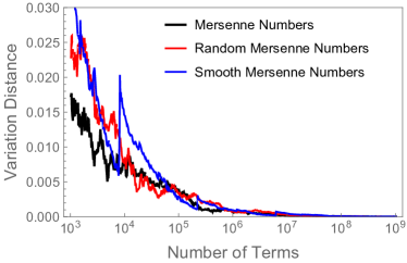
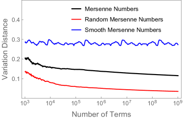
Figure 9. Variation distance between observed and predicted frequencies of $k$-tuples of leading digits for $k=1$ (left figure) and $k=2$ (right figure) in the sequence of Mersenne numbers, random Mersenne numbers, and smooth Mersenne numbers. When $k=1$, the variation distance approaches $0$ in all three cases. When $k=2$, the variation distance appears to approach $0$ for the Mersenne and random Mersenne numbers, but not for the smooth Mersenne numbers.

We conclude this section by commenting on the quality of the approximations in the local distribution of leading digits of Mersenne numbers predicted by Conjectures 2.7 and 2.8. As Figure 9 shows, while the variation distance for frequencies of pairs of leading digits of Mersenne numbers and of random Mersenne numbers both seem to converge to $0$, the rate of convergence is noticeably better for random Mersenne numbers. A similar difference in the quality of the fit can be observed in the distribution of pairs of leading digits in Table 5, and in the waiting time frequencies shown in Figure 5.

A plausible explanation for this difference in the quality of fit between Mersenne numbers and their random analogs is the slow rate of growth of the differences between consecutive primes, $p_{n+1}-p_{n}$, along with divisibility constraints of these differences. These constraints become negligible as $n\to\infty$, but they do have an influence when $n$ is small. For example, for $n\approx 10^{9}$, we expect the differences $p_{n+1}-p_{n}$ to be of average size $\log(10^{9})\approx 20$, and we expect differences between random primes to be of similar order of magnitude. However, for the prime numbers these differences must satisfy additional congruence constraints which significantly restrict the set of $k$-tuples of positive integers that may occur as $k$-tuples of differences between consecutive primes. For example, apart from finitely many exceptions, all elements in such a $k$-tuple of consecutive prime differences must be even, and no two consecutive elements can have the same non-zero remainder modulo $3$. For random primes there are no such constraints other than the restriction to integer values, thus causing random Mersenne numbers to have (initially) better Benford distribution properties on a local scale.

6. Proof of Theorem 2.9

Let $\{a_{n}\}$ be a sequence of positive real numbers satisfying the conditions (2.9) and (2.10) of the theorem. Setting

$$u_{n}=\Delta\log_{10}a_{n}=\log_{10}a_{n+1}-\log_{10}a_{n},$$

these conditions can be written as

(6.1) $$u_{n}\to\infty\quad(n\to\infty)$$

and

(6.2) $$u_{n+1}=u_{n}+O\left(\frac{1}{n}\right),$$

respectively.

Given a positive integer $k$, let $n_{k}$ denote the smallest integer $n$ with $u_{n}\geq k+1/2$. Then

(6.3) $$u_{n_{k}-1}<k+\frac{1}{2}\leq u_{n_{k}}.$$

By condition (6.1), $n_{k}$ is well-defined provided $k$ is sufficiently large, which we shall henceforth assume.

Conditions (6.2) and (6.3) imply

$$u_{n_{k}} =k+\frac{1}{2}+O\left(\frac{1}{n_{k}}\right)$$

and

$$u_{n} =k+\frac{1}{2}+O\left(\frac{n-n_{k}}{n_{k}}\right)\quad(n_{k}\leq n<2n_{k}).$$

It follows that, given $\epsilon>0$, there exists $\delta=\delta(\epsilon)>0$ such that, for sufficiently large $k$,

(6.4) $$\left|u_{n}-k-\frac{1}{2}\right|\leq\epsilon\quad(n_{k}\leq n<(1+\delta)n_{k}).$$

We now show that (6.4) is incompatible with the assumption that $\{a_{n}\}$ is locally Benford distributed of order $2$ (or greater), or that $\{a_{n}\}$ has Benford-distributed waiting times. Indeed, either of these assumptions implies that for all sufficiently large $k$ there exist integers $n$ with $n_{k}\leq n<(1+\delta)n_{k}$ such that $D(a_{n})=D(a_{n+1})=1$. The latter condition is equivalent to

$$\{\log_{10}a_{n}\}\in[0,\log_{10}2)\quad\text{and}\quad\{\log_{10}a_{n+1}\}\in[0,\log_{10}2).$$

Since $u_{n}=\log_{10}a_{n+1}-\log_{10}a_{n}$, it follows that if $D(a_{n})=D(a_{n+1})=1$, then

$$|u_{n}-m|\leq\log_{10}2=0.301\dots\quad\text{for some $m\in\mathbb{Z}$.}$$

This contradicts (6.4) upon choosing $\epsilon=0.1$. This completes the proof of Theorem 2.9.

7. Summary and Concluding Remarks

In this paper we presented the results of a large scale numerical investigation of the distribution of leading digits of the Mersenne numbers $M_{n}=2^{p_{n}}-1$, where $p_{n}$ is the $n$-th prime number. Our main empirical finding is that the leading digits of $\{M_{n}\}$ behave like a sequence of independent Benford-distributed random variables, on both a global and a local scale. The observed local behavior is in stark contrast to the behavior exhibited by other exponentially growing arithmetic sequences, which typically satisfy Benford’s Law on a global scale, but tend to have very poor local Benford distribution properties.

We have provided heuristic and numerical evidence suggesting that it is the statistical irregularities in the distribution of primes that cause the leading digit distribution of the Mersenne numbers, to be unusually regular. On the one hand, replacing the prime numbers $p_{n}$ by their smooth approximations $n\log n$ in the definition of $M_{n}$ yields a leading digit sequence that behaves similarly on a global scale, but has a completely different, and highly irregular, local behavior. On the other hand, replacing the prime numbers $p_{n}$ by appropriately defined “random primes” $p_{n}^{*}$ yields a behavior similar to that displayed by the Mersenne sequence.

This heuristic explanation for the “unreasonably” good fit of Benford’s Law to the sequence of Mersenne numbers is consistent with probabilistic explanations of Benford’s Law in terms of random processes such as repeated multiplications of random quantities; see, for example, Berger and Hill [7], Miller and Nigrini [29], and Chenavier et al. [12].

Our random model for Mersenne numbers is based on the classic Cramér model for the distribution of primes, in which the events “$n$ is prime”, $n=3,4,\dots$, are independent events, occurring with probability $1/\log n$. This essentially says that primes occur according to a Poisson process with interarrival times increasing at a rate $\log n$. Whether the actual sequence of primes behaves in this way is still conjectural, but Gallagher [17] (see also Soundararajan [35]) showed that, under the assumption of a generalized prime $k$-tuples conjecture, this is indeed the case. The close agreement between the leading digit behavior of the Mersenne numbers and that of a random analog of these numbers in which the primes are replaced by random primes can be seen as further evidence that the primes indeed behave according to a Poisson process.

We note that, for certain questions, Cramér’s model does not give the correct prediction for the behavior of primes. In particular, Maier [24] showed that the maximal gaps between prime numbers are significantly larger than those predicted by the model. However, these results do not affect the conjectured distribution of gaps based on the Poisson model; see the remark before Section 1.1 in Soundararajan [35].

To conclude this section, we comment on possible extensions and generalizations of the results and conjectures we have presented, and some open questions suggested by these results. The most obvious extension is to leading digits with respect to other bases. We expect all of our results and conjectures to remain valid for leading digits in a general base $b$, provided one excludes trivial situations such as bases that are powers of $2$.

Another natural extension is to sequences of the form $\{a^{p_{n}}\}$. Excluding trivial situations, we expect leading digits in these sequences to behave like those of the Mersenne numbers, $2^{p_{n}}-1$. For example, the proof of Theorem 2.5 shows that any sequence $\{a^{p_{n}}\}$ for which $\log_{10}a$ is irrational satisfies Benford’s Law. Similarly, we expect sequences of this form to have the same local Benford distribution properties as the sequence of Mersenne numbers.

Interestingly, this does not hold for the sequence of primorial numbers, $P_{n}=\prod_{k=1}^{n}p_{k}$, which have a similar rate of growth as the Mersenne numbers, $2^{p_{n}}-1$, but are more “smooth” at a local level. For example, we have $\log M_{n+1}-\log M_{n}\sim(\log 2)(p_{n+1}-p_{n}$), while $\log P_{n+1}-\log P_{n}=\log p_{n+1}$. Indeed, using an argument similar to that in the proof of Theorem 2.9, one can show that the sequence $\{P_{n}\}$ is not locally Benford distributed of order $2$ or larger.

The numerical data we presented in support of Conjecture 2.6 suggests the possibility that the error in the Benford approximation to leading digit counts of Mersenne numbers may be asymptotically normally distributed. This would represent a considerable strengthening of Conjecture 2.6.

A natural question is whether any of the conjectured results about the Mersenne numbers can be proved rigorously. Given our current state of knowledge on the distribution of primes, unconditional results seem unlikely; however, by following the method of Gallagher [17] it may be possible to prove Conjectures 2.7 and 2.8 conditionally, assuming an appropriate version of the prime $k$-tuples conjecture.

In this paper we focused on the distribution of the leading (i.e., leftmost) digit of $M_{n}$. One can ask more generally for the distribution of the $k$-th digit in the base $10$ (or base $b$) expansion of $M_{n}$. For fixed $k$, we expect similar results to hold, with the Benford distribution replaced by an appropriate analog for the $k$-th leading digit. More interesting is the case when $k$ is an increasing function of $n$. In this case, we expect the Benford phenomenon to gradually fade away as $k$ gets larger and the distribution to approach a uniform distribution. For example, it seems plausible that the distribution of the middle digits of the sequence of Mersenne numbers is asymptotically uniform, though results of this type appear to be out of reach given our current state of knowledge. On the other hand, the distribution of the rightmost digit (and, more generally, the $k$-th digit from the right) can be studied using exponential sums, and some results are known for the sequence of Mersenne numbers and similar exponentially growing sequences; see Banks et al. [3] and the references therein.

Acknowledgements.

We thank the referees for a careful reading of the paper and a number of comments that helped improve the paper.

References

- [1] Tom M. Apostol, Introduction to analytic number theory, Springer-Verlag, New York-Heidelberg, 1976, Undergraduate Texts in Mathematics. MR 0434929
- [2] William D. Banks and Igor E. Shparlinski, Prime numbers with Beatty sequences, Colloq. Math. 115 (2009), no. 2, 147–157.. MR 2491740
- [3] William D. Banks, John B. Friedlander, Moubariz Z. Garaev, and Igor E. Shparlinski, Exponential and character sums with Mersenne numbers, J. Aust. Math. Soc. 92 (2012), no. 1, 1–13. MR 2945673
- [4] Paul T. Bateman and Harold G. Diamond, Analytic number theory, Monographs in Number Theory, vol. 1, World Scientific Publishing Co. Pte. Ltd., Hackensack, NJ, 2004, An introductory course. MR 2111739
- [5] Nelson H. F. Beebe, A bibliography of publications about Benford’s law, Heap’s law and Zipf’s law, ftp://ftp.math.utah.edu/public_html/public_html/pub/tex/bib/benfords-law.pdf, 2017.
- [6] Frank Benford, The law of anomalous numbers, Proceedings of the American Philosophical Society 78 (1938), no. 4, 551–572.
- [7] Arno Berger and Theodore P. Hill, A basic theory of Benford’s law, Probab. Surv. 8 (2011), 1–126. MR 2846899
- [8] by same author, An introduction to Benford’s law, Princeton University Press, Princeton, NJ, 2015. MR 3242822
- [9] Arno Berger, Theodore P. Hill, and E. Rogers, Benford online bibliography, http://www.benfordonline.net, Last accessed 11.04.2017.
- [10] Zhaodong Cai, Matthew Faust, A. J. Hildebrand, Junxian Li, and Yuan Zhang, The unreasonable effectiveness of Benford’s Law in mathematics, Preprint.
- [11] Zhaodong Cai, A. J. Hildebrand, and Junxian Li, A local Benford Law for a class of arithmetic sequences, Preprint, http://arXiv.org/1808.01496.
- [12] Nicolas Chenavier, Bruno Massé, and Dominique Schneider, Products of random variables and the first digit phenomenon, Stochastic Processes and their Applications (2017), in press.
- [13] Daniel I. A. Cohen and Talbot M. Katz, Prime numbers and the first digit phenomenon, J. Number Theory 18 (1984), no. 3, 261–268. MR 746863
- [14] Persi Diaconis, The distribution of leading digits and uniform distribution , Ann. Probability 5 (1977), no. 1, 72–81. MR 0422186
- [15] S. Eliahou, B. Massé, and D. Schneider, On the mantissa distribution of powers of natural and prime numbers, Acta Math. Hungar. 139 (2013), no. 1-2, 49–63. MR 3028653
- [16] Aimé Fuchs and Giorgio Letta, Le problème du premier chiffre décimal pour les nombres premiers, Electron. J. Combin. 3 (1996), no. 2, Research Paper 25, The Foata Festschrift. MR 1392510
- [17] Patrick X. Gallagher, On the distribution of primes in short intervals, Mathematika 23 (1976), no. 1, 4–9. MR 0409385
- [18] Theodore P. Hill, The significant-digit phenomenon, Amer. Math. Monthly 102 (1995), no. 4, 322–327. MR 1328015
- [19] Werner Hürlimann, Generalizing Benford’s law using power laws: application to integer sequences, International Journal of Mathematics and Mathematical Sciences 2009 (2009), 45. MR 2533550
- [20] Werner Hürlimann, Benford’s law from 1881 to 2006: a bibliography, http://arxiv.org/ftp/math/papers/0607/0607168.pdf, Last accessed 11.04.2017.
- [21] Henryk Iwaniec and Emmanuel Kowalski, Analytic number theory, American Mathematical Society Colloquium Publications, vol. 53, American Mathematical Society, Providence, RI, 2004. MR 2061214
- [22] Lauwerens Kuipers and Harald Niederreiter, Uniform distribution of sequences, Wiley-Interscience [John Wiley & Sons], New York-London-Sydney, 1974, Pure and Applied Mathematics. MR 0419394
- [23] Bartolo Luque and Lucas Lacasa, The first-digit frequencies of prime numbers and Riemann zeta zeros, Proc. R. Soc. Lond. Ser. A Math. Phys. Eng. Sci. 465 (2009), no. 2107, 2197–2216. MR 2515637
- [24] Helmut Maier, Primes in short intervals, Michigan Math. J. 32 (1985), no. 2, 221–225. MR 783576
- [25] Bruno Massé and Dominique Schneider, A survey on weighted densities and their connection with the first digit phenomenon, Rocky Mountain J. Math. 41 (2011), no. 5, 1395–1415. MR 2838069
- [26] Bruno Massé and Dominique Schneider, The mantissa distribution of the primorial numbers, Acta Arith. 163 (2014), no. 1, 45–58. MR 3194056
- [27] Bruno Massé and Dominique Schneider, Fast growing sequences of numbers and the first digit phenomenon, International Journal of Number Theory 11 (2015), no. 705, 705–719. MR 3327839
- [28] Steven J. Miller (ed.), Benford’s Law: theory and applications, Princeton University Press, Princeton, NJ, 2015. MR 3408774
- [29] Steven J. Miller and Mark J. Nigrini, The modulo 1 central limit theorem and Benford’s law for products, Int. J. Algebra 2 (2008), no. 1-4, 119–130. MR 2417189
- [30] Norbert Müller, The iRRAM: Exact arithmetic in C++, Computability and Complexity in Analysis, Springer, 2001, pp. 222–252.
- [31] Simon Newcomb, Note on the frequency of use of the different digits in natural numbers, Amer. J. Math. 4 (1881), no. 1-4, 39–40. MR 1505286
- [32] Mark Nigrini, Benford’s law: Applications for forensic accounting, auditing, and fraud detection, vol. 586, John Wiley & Sons, 2012.
- [33] Ralph A. Raimi, The first digit problem, Amer. Math. Monthly 83 (1976), no. 7, 521–538. MR 0410850
- [34] Peter Schatte, On -summability and the uniform distribution of sequences, Math. Nachr. 113 (1983), 237–243. MR 725491
- [35] Kannan Soundararajan, The distribution of prime numbers, Equidistribution in number theory, an introduction, NATO Sci. Ser. II Math. Phys. Chem., vol. 237, Springer, Dordrecht, 2007, pp. 59–83. MR 2290494
- [36] I. M. Vinogradov, The method of trigonometrical sums in the theory of numbers, Trav. Inst. Math. Stekloff 23 (1947), 109. MR 0029417
- [37] Raymond E. Whitney, Initial digits for the sequence of primes, Amer. Math. Monthly 79 (1972), 150–152. MR 0304337