Statistical estimation in a randomly structured branching population

Abstract.

We consider a binary branching process structured by a stochastic trait that evolves according to a diffusion process that triggers the branching events, in the spirit of Kimmel’s model of cell division with parasite infection. Based on the observation of the trait at birth of the first $n$ generations of the process, we construct nonparametric estimator of the transition of the associated bifurcating chain and study the parametric estimation of the branching rate. In the limit $n\rightarrow\infty$, we obtain asymptotic efficiency in the parametric case and minimax optimality in the nonparametric case.

Mathematics Subject Classification (2010): 62G05, 62M05, 60J80, 60J20, 92D25.
Keywords: Branching processes, bifurcating Markov chains, statistical estimation, geometric ergodicity, scalar diffusions.

1. Introduction

1.1. Motivation

The study of structured populations, with a strong input from evolutionary or cell division modelling in mathematical biology (see for instance the textbooks [29, 32] and the references therein) has driven the statistics of branching Markov processes over the last few years. Several models have been considered, with data processed either in discrete or continuous time. In this context, one typically addresses the inference of critical parameters like branching rates, modelled as functions of biological traits like age, size and so on. In many cases, this approach is linked to certain piecewise deterministic Markov models or bifurcating Markov chains (BMC) in discrete time. These models are well understood from a probabilist point of view (in discrete time Guyon [19], Bitseki-Penda et al. [8, 9], in continuous time Bansaye and Méléard [4], Bansaye et al. [3] or more recently Marguet [28] for a general approach). For the statistical estimation, we refer to [10, 16, 17, 23, 5], and the references therein, see also Bitseki-Penda and Olivier [31], de Saporta et al. [14, 15], Azaïs et al. [1] or recently Bitseki-Penda and Roche [7]. In these models, the traits of a population between branching events like cell division evolve through time according to a dynamical system. The next logical step is to replace this deterministic evolution by a random flow, that allows one to account for traits that may have their own random evolution according to some exogeneous input. A paradigmatic example is Kimmel’s model (see Kimmel [24] and Bansaye [2]) where the trait is given by a density of parasites within a cell that evolve according to a diffusion process. The statistical analysis of such models is the topic of the present paper.

We consider a population model with binary division triggered by a trait $x\in\mathcal{X}$ where $\mathcal{X}\subseteq\mathbb{R}$ is an open (possibly unbounded) interval. The trait $\phi_{x}(t)$ of each individual evolves according to

(1) $$d\phi_{x}(t)=r(\phi_{x}(t))dt+\sigma(\phi_{x}(t))dW_{t},\;\;\phi_{x}(0)=x,$$

where $r,\sigma:\mathcal{X}\rightarrow\mathcal{X}$ are regular functions and $(W_{t})_{t\geq 0}$ is a standard Brownian motion. Each individual with trait $x$ dies according to a killing or rather division rate $x\mapsto B(x)$, i.e. an individual with trait $\phi_{x}(t)$ at time $t$ dies with probability $B(\phi_{x}(t))dt$ during the interval $[t,t+dt]$. At division, a particle with trait $y$ is replaced by two new individuals with trait at birth given respectively by $\theta y$ and $(1-\theta)y$ where $\theta$ is drawn according to $\kappa(y)dy$ for some probability density function $\kappa(y)$ on $[0,1]$.The model is described by the traits of the population, formally given as a Markov process

(2) $$X(t)=(X_{1}(t),X_{2}(t),\ldots),\;\;t\geq 0$$

with values in $\bigcup_{k\geq 1}\mathcal{X}^{k}$, where the $X_{i}(t)$ denote the (ordered) traits of the living particles at time $t$. Its distribution is entirely determined by an initial condition at $t=0$ and by the parameters $(r,\sigma,B,\kappa)$.

1.2. Statistical setting by reduction to a bifurcating Markov chain model

We assume we have data at branching events (i.e. at cell division) and we wish to make inference on the parameters of the model. Using the Ulam-Harris-Neveu notation, for $m\geq 0$, let $\mathbb{G}_{m}=\{0,1\}^{m}$ (with $\mathbb{G}_{0}=\{\emptyset\}$) and introduce the infinite genealogical tree

$$\mathbb{T}=\bigcup_{m\in\mathbb{N}}\mathbb{G}_{m}.$$

For $u\in\mathbb{G}_{m}$, set $|u|=m$ and define the concatenation $u0=(u,0)\in\mathbb{G}_{m+1}$ and $u1=(u,1)\in\mathbb{G}_{m+1}$. For $n\geq 0$, let $\mathbb{T}_{n}=\bigcup_{m=0}^{n}\mathbb{G}_{m}$ denote the genealogical tree up to the $n$-th generation and $|\mathbb{T}_{n}|$ denote its cardinality. We denote by $X_{u}$ the trait at birth of an individual $u\in\mathbb{T}$. From the branching events, we assume that we observe

$$\mathbb{X}^{n}=(X_{u})_{u\in\mathbb{U}_{n}},$$

where $\mathbb{U}_{n}\subseteq\mathbb{T}_{n}$ is what we call a regular incomplete tree, that is a connected subtree of $\mathbb{T}_{n}$ that contains at least one individual at the $n$-th generation (see the formal definition 8 in Section 2.2 below) and with cardinality of order $2^{\varrho n}$ for some $0\leq\varrho\leq 1$. This observation scheme is motivated by typical datasets available in biological experiments, see e.g. Robert et al. [34] and the refrences therein: when moving from generation $m-1$ to $m$ (for $m=1,\ldots,n$) we possibly lose some information, quantified by $\varrho$, due to experimental anomalies or simply because of the design of the experimental process (for instance, in the extreme case $\varrho=0$, it may well happen that one observes only a single lineage of the bifurcating process due to experimental constraints, as some datasets studied in [34]). We thus have approximately $2^{\varrho n}$ random variables with value in $\mathcal{X}$ with a certain Markov structure. Asymptotics are taken as $n$ grows to infinity. An example of trajectory is represented on Figure 1 with the associated genealogy.

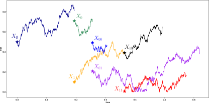
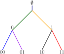
Figure 1. Example of a trajectory and its associated genealogy.

There are several objects of interest that we may try to infer from the data $\mathbb{X}^{n}$. First, one may notice that the Markov structure of $X$ in (2) turns $(X_{u},u\in\mathbb{T})$ into a bifurcating Markov chain according to the terminology introduced Basawa and Zhou [5], later highlighted by Guyon [19]. A bifurcating Markov chain is specified by 1) a measurable state space, here $\mathcal{X}$ (endowed with its Borel sigma-field) with a Markov kernel ${\mathcal{P}}$ from $\mathcal{X}$ to $\mathcal{X}\times\mathcal{X}$ and 2) a filtered probability space $\big{(}\Omega,\mathcal{F},(\mathcal{F}_{m})_{m\geq 0},\mathbb{P}\big{)}$. Following Guyon, [19], Definition 2, we have the

Definition 1.

A bifurcating Markov chain (BMC) is a family $(X_{u})_{u\in\mathbb{T}}$ of random variables with value in $\mathcal{X}$ such that $X_{u}$ is $\mathcal{F}_{|u|}$-measurable for every $u\in\mathbb{T}$ and

(3) $$\mathbb{E}\big{[}\prod_{u\in\mathbb{G}_{m}}\psi_{u}(X_{u},X_{u0},X_{u1})\,\big{|}\,\mathcal{F}_{m}\big{]}=\prod_{u\in\mathbb{G}_{m}}{\mathcal{P}}\psi_{u}(X_{u})$$

for every $m\geq 0$ and any family of (bounded) measurable functions $(\psi_{u})_{u\in\mathbb{G}_{m}}$, where ${\mathcal{P}}\psi(x)=\int_{\mathcal{X}\times\mathcal{X}}\psi(x,y_{1},y_{2}){\mathcal{P}}(x,dy_{1}dy_{2})$ denotes the action of ${\mathcal{P}}$ on $\psi$.

The distribution of $(X_{u})_{u\in\mathbb{T}}$ is thus entirely determined by ${\mathcal{P}}$ and an initial distribution for $X_{\emptyset}$. A key role for understanding the asymptotic behavior of the bifurcating Markov chain is the so-called tagged-branch chain, that consists in picking a lineage at random in the population $(X_{u})_{u\in\mathbb{T}}$: it is a Markov chain with value in $\mathcal{X}$ defined by $Y_{0}=X_{\emptyset}$ and for $m\geq 1$:

$$Y_{m}=X_{\emptyset\epsilon_{1}\ldots\epsilon_{m}},$$

where $(\epsilon_{m})_{m\geq 1}$ is a sequence of independent Bernoulli random variables with parameter $1/2$, independent of $(X_{u})_{u\in\mathbb{T}}$, with transition

(4) $$\mathcal{Q}=(\mathcal{P}_{0}+\mathcal{P}_{1})/2$$

obtained from the marginal transitions of $\mathcal{P}$:

$$\mathcal{P}_{0}(x,dy)=\int_{y_{1}\in\mathcal{X}}\mathcal{P}(x,dy\,dy_{1})\;\;\text{and}\;\;\mathcal{P}_{1}(x,dy)=\int_{y_{0}\in\mathcal{X}}\mathcal{P}(x,dy_{0}dy).$$

Guyon proves in [19] that if $(Y_{m})_{m\geq 0}$ is ergodic with invariant measure $\nu(dx)$ on $\mathcal{X}$, then a convergence of the type

(5) $$\frac{1}{|\mathbb{T}_{n}|}\sum_{u\in\mathbb{T}_{n}}\psi(X_{u},X_{u0},X_{u1})\rightarrow\int_{\mathcal{X}}\mathcal{P}\psi(x)\nu(dx)$$

holds as $n\rightarrow\infty$ for appropriate test functions $g$, almost surely and appended with appropriate central limit theorems (Theorem 19 in [19]). Under appropriate regularity assumptions, an analogous result shall hold when $\mathbb{T}_{n}$ is replaced by a regular incomplete tree $\mathbb{U}_{n}$.

1.3. Main results

In this context, there are several quantities that can be inferred from the data $\mathbb{X}_{n}$ as $n$ grows and that are important in order to understand the dynamics of $(X_{u})_{u\in\mathbb{T}}$. Under suitable assumptions on the stochastic flow (1), the transition $\mathcal{Q}$ admits an invariant measure $\nu$ and we have fast convergence of the tagged-chain $(Y_{m})_{m\geq 1}$ to equilibrium. This enables us to construct in a first part nonparametric estimators of $\nu$ and $\mathcal{Q}$ with an optimal rate of convergence and reveals the structure of the underlying BMC.

However, estimators of $\nu$ and $\mathcal{Q}$ do not give us any insight about the parameters $(r,\sigma,B,\kappa)$ of the model. In a second part, we investigate the inference of the division rate $x\mapsto B(x)$ as a function of the trait $x\in\mathcal{X}$ when the other parameters $r,\sigma$ and $\kappa(x)$ are known. This seemingly stringent assumption is necessary given the observation scheme $\mathbb{X}^{n}$. If extraneous data were available, estimators of the parameters $r,\sigma$ and $\kappa$ could be obtained in a relatively straightforward manner:

• As soon as a discretisation of the values of the flow are available, standard techniques about inference in ergodic diffusions can be applied to recover $x\mapsto r(x)$ and $x\mapsto\sigma(x)^{2}$, see for instance [22, 25].

• The fact that an individual $u$ distributed its traits to its offspring in a conservative way enables one to recover the fraction $\theta_{u}$ distributed among the children. Indeed the individual $u$ born at $b_{u}$ with lifespan $d_{u}-b_{u}$ has trait $\phi_{X_{u}}(d_{u}-b_{u})$ at its time of death. It follows that its children have trait at birth given by

  $$X_{u0}=\theta_{u}\phi_{X_{u}}(d_{u}-b_{u}),\;\;X_{u1}=(1-\theta_{u})\phi_{X_{u}}(d_{u}-b_{u}),$$

  where the $\theta_{u}$ are drawn independently from the distribution $\kappa(x)dx$ and therefore, the relationship $\frac{X_{u_{0}}}{X_{u_{1}}}=\frac{\theta_{u}}{1-\theta_{u}}$ identifies $\theta_{u}$. In turn, the estimation of $x\mapsto\kappa(x)$ reduces to a standard density estimation problem from data $(\theta_{u})_{u\in\mathbb{U}_{n}}$, see for instance [21].

The identification and estimation of the branching rate $x\mapsto B(x)$ from data $\mathbb{X}^{n}$ is more delicate and is the topic of the second part of the paper. Under minimal regularity assumptions developed in Section 2 below, it is not difficult to obtain an explicit representation of the transition $\mathcal{Q}(x,dy)=\mathcal{Q}_{B}(x,dy)=q_{B}(x,y)dy$ that reads

(6) $$q_{B}(x,y)=\int_{0}^{1}\Big{(}\frac{\kappa(z)+\kappa(1-z)}{2z}\Big{)}B(y/z)\sigma(y/z)^{-2}\mathbb{E}\Big{[}\int_{0}^{\infty}e^{-\int_{0}^{t}B(\phi_{x}(s))ds}dL_{t}^{y/z}(\phi_{x})\Big{]}dz,$$

where $L_{t}^{y}(\phi_{x})$ denotes the local time at $t$ in $y$ of the semimartingale $(\phi_{x}(t))_{t\geq 0}$. Assuming $(r,\sigma,\kappa)$ known (or identified by extraneous observation schemes) we study the estimation of $x\mapsto B(x)$ when $B$ belongs to a parametric class of functions $\{B_{\vartheta},\vartheta\in\Theta\}$ for some regular subset of the Euclidean space $\mathbb{R}^{d}$. Under a certain ordering property (Definition 15 in Section 3.2 below) that ensures identifiability of the model and suitable standard regularity properties, we realise a standard maximum likelihood proxy estimation of $B$ thanks to (6) by maximising the contrast

$$\vartheta\mapsto\prod_{u\in\mathbb{U}_{n}^{\star}}q_{B_{\vartheta}}(X_{u^{-}},X_{u}),\;\;\vartheta\in\Theta,$$

(with $\mathbb{U}_{n}^{\star}=\mathbb{U}_{n}\setminus\mathbb{G}_{0}$ and where $u^{-}$ denotes the unique parent of $u$) and we prove that it achieves asymptotic efficiency and discuss its practical implementation. It is noteworthy that for the parametric estimation of $B$, there is no straightforward contrast minimisation procedure (at least we could not find any) whereas $q_{B}(x,y)$ is explicit. The fairly intricate dependence of $B$ in the representation (6) makes however the whole scheme relatively delicate, both mathematically and numerically.

Clearly, other observation schemes are relevant in the context of cell division modelling. For instance, one could consider a (large) time $T>0$ and observe the branching process $X_{t}$ defined in (2) for every $t\in[0,T]$. This entails the possibility to extract the times $(T_{u})$ at which branching events occur, like e.g. in [23]. However, the continuous time setting is drastically different and introduce the additional difficulty of bias sampling, an issue we avoid in the present context. Alternatively, one could consider the augmented statistical experiment where one observes $(X_{u},T_{u})_{u\in{\mathbb{U}}_{n}}$, but the underlying mathematical structure is presumably not simpler. Our results show in particular that for the parametric estimation of the branching rate $B$, although the times at which branching event occur are statistically informative, their observation is not necessary to obtain optimal rates of convergence as soon as $(r,\sigma,\kappa)$ are known.

1.4. Organisation of the paper

Section 2.1 is devoted to the construction of the stochastic model, our assumptions and the accompanying statistical experiments. In particular, we have a nice structure enough so that explicit representations of $\mathcal{P}$ and $\mathcal{Q}$ are available (Proposition 5). We give a first result on the geometric ergodicity of the model via an explicit Lyapunov function in Proposition 6 and derive in Proposition 9 a rate of convergence for the variance of empirical measures of the data $\mathbb{X}^{n}=(X_{u})_{u\in\mathbb{U}_{n}}$ against test functions $\varphi(X_{u})$ or $\psi(X_{u^{-}},X_{u})$ with a sharp control in terms of adequate norms for $\varphi,\psi$ that do not follow from the standard application of the geometric ergodicity of Proposition 6. This is crucial for the subsequent applications to the nonparametric estimation of $\mathcal{Q}$ and its invariant measure $\nu$ that are given in Theorem 12 of Section 3.1. Section 3.2 is devoted to the parametric estimation of the branching rate, where an asymptotically efficient result is proved for a maximum likelihood estimator in Theorem 22. It is based on a relatively sharp study of the transition $\mathcal{Q}$, thanks to local time properties of the stochastic flow that triggers the branching events. Section 4 is devoted to the numerical implementation of the parametric estimator of $B$. In particular, in order to avoid the computational cost of the explicit computation of $q_{\vartheta}(X_{u^{-}},X_{u})$, we take advantage of our preceding results and implement a nonparametric estimator on Monte-Carlo simulations instead, resulting in a feasible procedure for practical purposes. The proofs are postponed to Section 5 and an Appendix Section 6 contains useful auxiliary results.

2. A cell division model structured by a stochastic flow

2.1. Assumptions and well-posedness of the stochastic model

Dynamics of the traits

Remember that $\mathcal{X}\subseteq\mathbb{R}$ is an open, possibly unbounded interval. The flow is specified by $r,\sigma:\mathcal{X}\rightarrow\mathcal{X}$ which are measurable and that satisfy the following assumption:

Assumption 2.

For some $r_{1},\sigma_{1},\sigma_{2}>0$, we have $|r(x)|\leq r_{1}(1+|x|)$ and $\sigma_{1}\leq\sigma(x)\leq\sigma_{2}$, for every $x\in\mathcal{X}$. Moreover, for some $r_{2}>0$, we have $\operatorname*{sgn}(x)r(x)<0$ for $|x|\geq r_{2}$ (with $\operatorname*{sgn}(x)=\mathbf{1}_{\{x>0\}}-\mathbf{1}_{\{x\leq 0\}}$).

Under Assumption 2, there is a unique strong solution to (1) (for instance [30], Theorem 5.2.1.). We denote by $\left(\Phi_{x}(t),t\geq 0\right)$ the unique solution to (1) with initial condition $x\in\mathcal{X}$. In particular, $\left(\Phi_{x}(t),t\geq 0\right)$ is a strong Markov process and is ergodic (cf. [25], Theorem 1.16.). Note that when $\mathcal{X}$ is bounded, the drift condition $\operatorname*{sgn}(x)r(x)<0$ for large enough $x$ can be dropped.

Division events.

An individual with trait $x$ dies at an instantaneous rate $x\mapsto B(x)$, where $B:\mathcal{X}\rightarrow[0,\infty)$ satisfies the following condition:

Assumption 3.

The function $x\mapsto B(x)$ is continuous. Moreover, for some $b_{1},b_{2}>0$ and $\gamma\geq 0$, we have $b_{1}\leq B(x)\leq b_{2}\left|x\right|^{\gamma}+b_{1}$ for every $x\in\mathcal{X}$.

Under Assumptions 2 and 3, the process $X$ in (2) is well defined and the size of the population does not explode in finite time almost-surely, see for instance Marguet [28]. Note that the lower bounds for $\sigma$ and $B$ are not needed for the well-posedness of $X$ but rather for later statistical purposes.

Fragmentation of the trait at division

Finally, we make an additional set of assumptions on the fragmentation distribution $\kappa(z)dz$ that ensures in particular the non-degeneracy of the process.

Assumption 4.

We have

• $\mathrm{supp}(\kappa)\subset[\varepsilon,1-\varepsilon]$ for some $0<\varepsilon<1/2$,

• $\inf_{z\in[\varepsilon,1-\varepsilon]}\kappa(z)\geq\delta$.

This assumption is slightly technical and may presumably be relaxed. We emphasize that the density $\kappa(z)$ needs not be symmetric.

Representations of $\mathcal{P}$ and $\mathcal{Q}$

Under Assumptions 2, 3 and 4, we obtain closed-form formulae for the transition $\mathcal{P}$ defined via (3) and the mean or marginal transition $\mathcal{Q}$ of the BMC $(X_{u})_{u\in\mathbb{T}}$, see (4) that also gives the transition probability of the discrete Markov chain with value in $\mathcal{X}$ corresponding to the trait at birth along an ancestral lineage. These representations are crucial for the subsequent analysis of the variance of the estimators of $\mathcal{P}$ and of the invariant measure $\nu$.

Proposition 5.

Work under Assumptions 2, 3 and 4. For every $x,y,y_{1},y_{2}\in\mathcal{X}$, we have

$$\mathcal{P}(x,dy_{1}dy_{2})=p(x,y_{1},y_{2})dy_{1}dy_{2}\;\;\text{and}\;\;\mathcal{Q}(x,dy)=q(x,y)dy,$$

with

(7) $$p(x,y_{1},y_{2})=\frac{\kappa\big{(}y_{1}/(y_{1}+y_{2})\big{)}}{y_{1}+y_{2}}B\left(y_{1}+y_{2}\right)\sigma(y_{1}+y_{2})^{-2}\mathbb{E}\Big{[}\int_{0}^{\infty}e^{-\int_{0}^{t}B(\phi_{x}(s))ds}dL_{t}^{y_{1}+y_{2}}(\phi_{x})\Big{]}$$

and

(8) $$q(x,y)=\int_{0}^{1}\frac{\widetilde{\kappa}(z)}{z}B(y/z)\sigma(y/z)^{-2}\mathbb{E}\Big{[}\int_{0}^{\infty}e^{-\int_{0}^{t}B(\phi_{x}(s))ds}dL_{t}^{y/z}(\phi_{x})\Big{]}dz,$$

where $\widetilde{\kappa}(z)=\tfrac{1}{2}(\kappa(z)+\kappa(1-z))$ and $L_{t}^{y}(\phi_{x})$ denotes the local time at $t$ in $y$ of the semimartingale $(\phi_{x}(t))_{t\geq 0}$.

Notice that in the case of a symmetric fragmentation kernel, we have $\widetilde{\kappa}=\kappa$.

2.2. Convergence of empirical measures

We study the convergence of empirical means of the form

(9) $$\mathcal{M}_{\mathbb{U}_{n}}(\psi)=\frac{1}{|\mathbb{U}_{n}^{\star}|}\sum_{u\in\mathbb{U}_{n}^{\star}}\psi(X_{u^{-}},X_{u})$$

towards $\nu\mathcal{Q}(\psi)$ if $\mathbb{U}_{n}$ is a rich enough incomplete tree, for test functions $\psi:\mathcal{X}\times\mathcal{X}\rightarrow\mathbb{R}$. (If $\varphi:\mathcal{X}\rightarrow\mathbb{R}$ we set $\mathcal{M}_{\mathbb{U}_{n}}(\varphi)=|\mathbb{U}_{n}|^{-1}\sum_{u\in\mathbb{U}_{n}}\varphi(X_{u})\rightarrow\nu(\varphi)$ and we have a formal correspondence between the two expressions by writing $\psi(x,y)=\varphi(y)$ as a function of the second variable.) In order to derive nonparametric estimators of $\nu$ and $\mathcal{Q}$ by means of kernel functions $\psi$ that shall depend on $n$, we need sharp estimates in terms of $\psi$, see Remark 1) after Proposition 9 below.

Convergence of $\mathcal{Q}$ to equilibrium

Assumptions 2, 3 and 4 imply a drift condition for the Lyapunov function $V(x)=x^{2}$ on $\mathcal{X}$ and a minorisation condition over a small set so that in turn $\mathcal{Q}$ is geometrically ergodic.

Let $\mathbb{Q}=\mathbb{Q}(r_{i},b_{i},\sigma_{i},\gamma,\varepsilon,\delta,i=1,2)$ be the class of all transitions $\mathcal{Q}=\mathcal{Q}(r,\sigma,B,\kappa)$ defined over $\mathcal{X}$ that satisfy Assumptions 2, 3 and 4 with appropriate constants. An invariant probability measure for $\mathcal{Q}$ is a probability $\nu$ on $\mathcal{X}$ such that $\nu\mathcal{Q}=\nu$, where $\nu\mathcal{Q}(dy)=\int_{x\in\mathcal{X}}\nu(dx)\mathcal{Q}(x,dy)$. Define

$$\mathcal{Q}^{r}(x,dy)=\int\mathcal{Q}(x,dz)\mathcal{Q}^{r-1}(z,dy)\;\;\text{with}\;\;\mathcal{Q}^{0}(x,dy)=\delta_{x}(dy)$$

for the $r$-th iteration of $\mathcal{Q}$. For $\varphi:\mathcal{X}\rightarrow\mathbb{R}$, we set

$$|\varphi|_{V}=\sup_{x\in\mathcal{X}}\frac{|\varphi(x)|}{1+V(x)}$$

and write $\nu(\varphi)=\int_{\mathcal{X}}\varphi(x)\nu(dx)$ when no confusion is possible.

Proposition 6 (Convergence to equilibrium).

Work under Assumptions 2, 3 and 4. Then any $\mathcal{Q}\in\mathbb{Q}$ admits an invariant probability distribution $\nu$. Moreover, for $V(x)=x^{2}$, there exist $C=C(\mathcal{Q})>0$ and $\rho=\rho(\mathcal{Q})\in(0,1)$ such that for every $m\geq 1$, the bound

$$\big{|}\mathcal{Q}^{m}\varphi-\nu(\varphi)\big{|}_{V}\leq C\rho^{m}\big{|}\varphi-\nu(\varphi)\big{|}_{V}$$

holds as soon as $|\varphi|_{V}<\infty$. Moreover, $\sup_{\mathcal{Q}\in\mathbb{Q}}C(\mathcal{Q})<\infty$ and $\sup_{\mathcal{Q}\in\mathbb{Q}}\rho(\mathcal{Q})<1$.

In particular, if $|\varphi|_{\infty}=\sup_{x\in\mathcal{X}}|\varphi(x)|$ is finite, we have $\left|\mathcal{Q}^{m}\varphi(x)-\nu(\varphi)\right|\leq C\rho^{m}(1+V(x))|\varphi-\nu(\varphi)|_{\infty}$ for every $x\in\mathcal{X}$.

Sharp controls of empirical variances

Proposition 6 is the key ingredient in order to control the rate of convergence of empirical means of the form (9) for appropriate observation schemes $\mathbb{U}_{n}\subset\mathbb{T}_{n}$.

We need some notation. We denote by $|\cdot|_{1}$ the usual $L^{1}$-norm w.r.t. the Lebesgue measure on $\mathcal{X}\times\mathcal{X}$. For a function $\psi=\mathcal{X}\times\mathcal{X}\rightarrow\mathbb{R}$ we set $\psi^{\star}(x)=\sup_{y\in\mathcal{X}}|\psi(x,y)|$ and $\psi_{\star}(y)=\sup_{x\in\mathcal{X}}|\psi(x,y)|$ and define

$$|\psi|_{\wedge 1}=\min\Big{(}\int_{\mathcal{X}\times\mathcal{X}}|\psi(x,y)|dxdy,\int_{\mathcal{X}}\sup_{x\in\mathcal{X}}|\psi(x,y)|dy\Big{)}.$$

Note in particular that when $\psi(x,y)=\varphi(y)$ is a function of $y$ only, we may have that $|\psi_{\star}|_{1}=\int_{\mathcal{X}}|\varphi(y)|dy$ is finite while $\psi$ is not integrable on $\mathcal{X}\times\mathcal{X}$ as a function of two variables. For a positive measure $\rho$ on $\mathcal{X}$, let also

$$|\psi|_{\rho}=\int_{\mathcal{X}\times\mathcal{X}}|\psi(x,y)|\rho(dx)dy+|\psi|_{\wedge 1}.$$

We write $\mathbb{P}_{\mu}$ for the law of $(X_{u})_{u\in\mathbb{T}}$ with initial distribution $\mu$ for $X_{\emptyset}$. Remember that $V(x)=x^{2}$ from Proposition 6. We shall further restrict our study to transitions $\mathcal{Q}\in\mathbb{Q}$ for which the geometric rate of convergence to equilibrium $\rho=\rho(\mathcal{Q})$ given in Proposition 6 satisfies $\rho(\mathcal{Q})\leq 1/2$. Let $\mathbb{Q}_{1/2}\subset\mathbb{Q}$ denote the set of such transitions.

Remark 7.

It is delicate to check in general that $\rho\leq 1/2$ but it is for instance satisfied in the following example:

• $\phi_{x}(t)$ is an Ornstein-Uhlenbeck process on $\mathcal{X}=\mathbb{R}$: we have $r(x)=-\beta x$ and $\sigma(x)=\sigma$ for every $x\in\mathcal{X}$ and some $\beta,\sigma>0$,

• the division rate is constant: we have $B(x)=b$ for every $x\in\mathcal{X}$ and some $b>0$,

• the fragmentation distribution is uniform: we have $\kappa(z)=1/(1-2\varepsilon)$ on $[\varepsilon,1-\varepsilon]$ for some $\varepsilon>0$.

Adapting the proof of Proposition 24 below to this special case and using the explicit formula of $\rho$ given Theorem 1.2 in [20], we show in Appendix 6.1 that for $B$ small enough, we have $\rho<1/2$ in this example.

Finally we consider observation schemes $\mathbb{U}_{n}$ that satisfy a certain sparsity condition that we quantify in the following definition

Definition 8.

A regular incomplete tree is a subset $\mathbb{U}_{n}\subseteq\mathbb{T}_{n}$ (for $n\geq 1$) such that

• $u\in\mathbb{U}_{n}$ implies $u^{-}\in\mathbb{U}_{n}$,

• We have $0<\liminf_{n\rightarrow\infty}2^{-n\varrho}\big{|}\mathbb{U}_{n}\cap\mathbb{G}_{n}\big{|}\leq\limsup_{n\rightarrow\infty}2^{-n\varrho}\big{|}\mathbb{U}_{n}\cap\mathbb{G}_{n}\big{|}<\infty$ for some $0\leq\varrho\leq 1$.

Proposition 9.

Work under Assumptions 2, 3 and 4. Let $\mu$ be a probability measure on $\mathcal{X}$ such that $\mu(V^{2})<\infty$. Let $\psi:\mathcal{X}\times\mathcal{X}\rightarrow\mathbb{R}$ a bounded function such that $\psi_{\star}$ is compactly supported. If $\mathbb{U}_{n}$ is a regular incomplete tree, the following estimate holds true:

$$\mathbb{E}_{\mu}\big{[}\big{(}\mathcal{M}_{\mathbb{U}_{n}}(\psi)-\nu(\mathcal{Q}\psi)\big{)}^{2}\big{]} \lesssim|\mathbb{U}_{n}|^{-1}\big{(}|\psi^{2}|_{\mu+\nu}+|\psi^{\star}\psi|_{\mu}+\big{(}1+\mu(V^{2})\big{)}|\psi_{\star}|_{1}|\psi|_{\nu}\big{)},$$

where the symbol $\lesssim$ means up to an explicitly computable constant that depends on $\mathcal{Q}$ and on $\text{supp}(\psi_{\star})$ only. Moreover, the estimate is uniform in $\mathcal{Q}\in\mathbb{Q}_{1/2}$.

Several remarks are in order: 1) We have a sharp order in terms of the test functions $\psi$, that behave no worse than $\int_{\mathcal{X}^{2}}\psi^{2}$ under minimal regularity on $\nu$ which is satisfied, see Lemma 27 below (and of course $\mu$, although this restriction could be relaxed). This behaviour is the one expected for instance in the IID case and is crucial for the subsequent statistical application of Theorem 12 where the functions $\psi$ will be kernel depending on $n$. 2) The proof heavily relies on the techniques developed in Biteski Penda et al. [8] or Guyon [19] (more specifically, Theorems 11 and 12 of [19] or Theorem 2.11 and 2.1 of [8], see also [10, 7]). However, we need a slight refinement here, in order to obtain a sharp control in terms of the trial function $\psi$, similar to the behaviour of $\int_{\mathcal{X}^{2}}\psi^{2}$, while the aformentioned references would give a term of order $\sup_{x,y}|\psi(x,y)|$ that would not be sufficiently sharp for the nonparametric statistical analysis. 3) Proposition 9 has an analog in [17] for piecewise deterministic growth-fragmentation models, but our proof is somewhat simpler here and sharper (we do not pay the superfluous logarithmic term in [17]). 4) Finally, note that in Proposition 9, the observation $\mathbb{U}_{n}$ must be deterministic (or at least independent of $(X_{u})_{u\in\mathbb{T}_{n}}$) otherwise biased selection may occur that would result in completely different behaviours of the empirical means (like for instance if $\mathbb{U}_{n}$ is allowed to contain stopping times on the tree).

3. Statistical estimation

3.1. Nonparametric estimation of $\mathcal{Q}$ and $\nu$

Under Assumptions 2, 3 and 4, any $\mathcal{Q}(x,dy)=q(x,y)dy$ admits an invariant probability measure $\nu(dx)=\nu(x)dx$, the regularity of $\nu(x)$ being inherited from that of $\mathcal{Q}$ via $\nu(x)=\int_{\mathcal{X}}q(z,x)\nu(dz)$.

Fix $(x_{0},y_{0})\in\mathcal{X}\times\mathcal{X}$. We are interested in constructing estimators of $q(x_{0},y_{0})$ and $\nu(x_{0})$ from the observation $\mathbb{X}^{n}$ when both functions satisfy some Hölder regularity properties in the vicinity of $(x_{0},y_{0})$. To that end, we need approximating kernels.

Definition 10.

A function $G:\mathcal{X}\rightarrow\mathbb{R}$ is a kernel of order $k$ if it is compactly supported and satisfies $\int_{\mathcal{X}}x^{\ell}G(x)dx={\bf 1}_{\{\ell=0\}}$ for $\ell=0,\ldots,k$.

The construction and numerical tractability of approximating kernels is documented in numerous textbooks, see for instance Tsybakov [36, Chapter 1]. For bandwidth parameters $h,h_{1},h_{2}>0$, we set

$$G_{h}(y)=h^{-1}G(h^{-1}y)$$

and

$$G^{\otimes 2}_{h_{1},h_{2}}(x,y)=h_{1}^{-1}h_{2}^{-1}G(h_{1}^{-1}x)G(h_{2}^{-1}y\big{)}$$

and obtain approximations of $\nu(y_{0})$ and $q(x_{0},y_{0})$ by setting

$$G_{h}\star\nu(y_{0})=\int_{\mathcal{X}}G_{h}(y_{0}-y)\nu(y)dy$$

and

$$G_{h}\star q(x_{0},y_{0})=\int_{\mathcal{X}\times\mathcal{X}}G_{h_{1},h_{2}}^{\otimes 2}(x_{0}-x,y_{0}-y)\nu(x)q(x,y)dxdy.$$

The convergence of $\mathcal{M}_{\mathbb{U}_{n}}(\varphi)$ to $\nu(\varphi)$ suggests to pick $\varphi=G_{h}(x_{0}-\cdot)$. Then $\mathcal{M}_{\mathbb{U}_{n}}(G_{h}(x_{0}-\cdot))$ is close to $G_{h}\star\nu(x_{0})$ for small enough $h$ and can be used as a proxy of $\nu(x_{0})$. We obtain the estimator

$$\widehat{\nu}_{n}(x_{0})=\mathcal{M}_{\mathbb{U}_{n}}\big{(}G_{h}(x_{0}-\cdot)\big{)},$$

specified by the choice of $h>0$ and the kernel $G$. Likewise, with $\psi=G_{h_{1},h_{2}}(x_{0}-\cdot,y_{0}-\cdot)$, an estimator of $q(x_{0},y_{0})$ is obtained by considering the quotient estimator with numerator $\mathcal{M}_{\mathbb{U}_{n}}(\psi)$ that is close to $G_{h_{1},h_{2}}\star\big{(}\nu(\cdot)q(\cdot,\cdot)\big{)}(x_{0},y_{0})$ and denominator $\widehat{\nu}_{n,h}(x_{0})$ in order to balance the superfluous weight $\nu(x_{0})$ in the numerator. We obtain the estimator

$$\widehat{q}_{n}(x_{0},y_{0})=\frac{\mathcal{M}_{\mathbb{U}_{n}}\big{(}G_{h_{1},h_{2}}^{\otimes 2}(x_{0}-\cdot,y_{0}-\cdot)\big{)}}{\mathcal{M}_{\mathbb{U}_{n}}\big{(}G_{h}(x_{0}-\cdot)\big{)}\vee\varpi},$$

specified by the choice of $h,h_{1},h_{2}>0$, a threshold $\varpi>0$ and the kernel $G$. In order to quantify the kernel approximation, we introduce anisotropic Hölder classes. For $\alpha>0$, we write $\alpha=\lfloor\alpha\rfloor+\{\alpha\}$ with $\lfloor\alpha\rfloor$ an integer and $0<\{\alpha\}\leq 1$.

Definition 11.

Let $\alpha,\beta>0$ and $\mathcal{V}_{x_{0}}$ and $\mathcal{V}_{y_{0}}$ be bounded neighbourhoods of $x_{0}$ and $y_{0}$.

• The function $\varphi:\mathcal{V}_{x_{0}}\rightarrow\mathbb{R}$ belongs to the Hölder class $\mathcal{H}^{\alpha}(x_{0})$ if

  (10) $$|\varphi^{(\lfloor\alpha\rfloor)}(y)-\varphi^{(\lfloor\alpha\rfloor)}(x)|\leq C|y-x|^{\{\alpha\}}\;\;\text{for every}\;\;x,y\in\mathcal{V}_{x_{0}}.$$

• The function $\psi:\mathcal{V}_{x_{0}}\times\mathcal{V}_{y_{0}}\rightarrow\mathbb{R}$ belongs to the anisotropic Hölder class $\mathcal{H}^{\alpha,\beta}(x_{0},y_{0})$ if

  $$x\mapsto\psi(x,y_{0})\in\mathcal{H}^{\alpha}(x_{0})\;\;\text{and}\;\;y\mapsto\psi(x_{0},y)\in\mathcal{H}^{\beta}(y_{0})$$

  hold simultaneously.

We obtain a semi-norm on $\mathcal{H}^{\alpha}(x_{0})$ by setting $|\varphi|_{\mathcal{H}^{\alpha}(x_{0})}=\sup_{x\in\mathcal{V}_{x_{0}}}|\varphi(x)|+c_{\alpha}(\varphi),$ where $c_{\alpha}(\varphi)$ is the smallest constant for which (10) holds. Likewise, we equip $\mathcal{H}^{\alpha,\beta}(x_{0},y_{0})$ with the semi-norm $|\psi|_{\mathcal{H}^{\alpha,\beta}(x_{0},y_{0})}=|\psi(\cdot,y_{0})|_{\mathcal{H}^{\alpha}(x_{0})}+|\psi(x_{0},\cdot)|_{\mathcal{H}^{\beta}(y_{0})}$. The space $\mathcal{H}^{\alpha,\beta}(x_{0},y_{0})$ is appended with (semi) Hölder balls

$$\mathcal{H}^{\alpha,\beta}(x_{0},y_{0})(R)=\big{\{}\psi:\mathcal{X}\times\mathcal{X}\rightarrow\mathbb{R},|\psi|_{\mathcal{H}^{\alpha,\beta}(x_{0},y_{0})}\leq R\big{\}},\;\;R>0.$$

We are ready to state our convergence result over transitions $\mathcal{Q}$ that belong to

$$\mathbb{Q}_{1/2}^{\alpha,\beta}(R)=\mathbb{Q}_{1/2}\cap\mathcal{H}^{\alpha,\beta}(x_{0},y_{0})(R),\;\;R>0,$$

with a slight abuse of notation.

Theorem 12.

Work under Assumptions 2, 3 and 4. Assume that the initial distribution $\mu$ is absolutely continuous w.r.t. the Lebesgue measure with a locally bounded density function and satisfies $\mu(V^{2})<\infty$.

Let $\alpha,\beta>0$. Specify $\widehat{\nu}_{n}(y_{0})$ by a kernel of order $k>\max\{\alpha,\beta\}$ and $h=|\mathbb{U}_{n}|^{-1/(2\beta+1)}$ and $\widehat{q}_{n}(x_{0},y_{0})$ with the same kernel and $h_{1}=|\mathbb{U}_{n}|^{-s(\alpha,\beta)/(\alpha\wedge\beta)(2s(\alpha,\beta)+1)}$, $h_{2}=|\mathbb{U}_{n}|^{-s(\alpha,\beta)/\beta(2s(\alpha,\beta)+1)}$ and $\varpi=\varpi_{n}\rightarrow 0$. Then, if $\mathbb{U}_{n}$ is an $\varrho$-regular incomplete tree, for every $R>0$,

$$\sup_{\mathcal{Q}\in\mathbb{Q}_{1/2}^{\alpha,\beta}(R)}\big{(}\mathbb{E}_{\mu}\big{[}\big{(}\widehat{\nu}_{n}(y_{0})-\nu(y_{0})\big{)}^{2}\big{]}\big{)}^{1/2}\lesssim|\mathbb{U}_{n}|^{-\beta/(2\beta+1)}$$

and

$$\sup_{\mathcal{Q}\in\mathbb{Q}_{1/2}^{\alpha,\beta}(R)}\big{(}\mathbb{E}_{\mu}\big{[}\big{(}\widehat{q}_{n}(x_{0},y_{0})-q(x_{0},y_{0})\big{)}^{2}\big{]}\big{)}^{1/2}\lesssim\varpi_{n}^{-1}|\mathbb{U}_{n}|^{-s(\alpha,\beta)/(2s(\alpha,\beta)+1)}$$

hold true, where $s(\alpha,\beta)^{-1}=(\alpha\wedge\beta)^{-1}+\beta^{-1}$ is the effective anisotropic smoothness associated with $(\alpha,\beta)$.

Several remarks are in order: 1) We obtain an optimal result in the minimax sense for estimating $\nu(y_{0})$ and in the case $\beta\geq\alpha$ for estimating $q(x_{0},y_{0})$. This stems from the fact that the representation $\nu(x)=\int_{\mathcal{X}}\nu(y)q(y,x)dy$ henceforth $q\in\mathcal{H}^{\alpha,\beta}$ implies that $\nu\in\mathcal{H}^{\beta}$. In turn, the numerator of $\widehat{q}_{n}(x_{0},y_{0})$ is based on the estimation of the function $\nu(x)q(x,y)\in\mathcal{H}^{\alpha\wedge\beta,\beta}$. 2) In the estimation of $q(x_{0},y_{0})$, we have a superfluous term $\varpi_{n}^{-1}$ in the error that can be taken arbitrarily small, and that comes from the denominator of the estimator. It can be removed, however at a significant technical cost. Alternatively, one can get rid of it by weakening the error loss: it is not difficult to prove

$$\big{(}\mathbb{E}_{\mu}\big{[}\big{(}\widehat{q}_{n}(x_{0},y_{0})-q(x_{0},y_{0})\big{)}^{p}\big{]}\big{)}^{1/p}\lesssim|\mathbb{U}_{n}|^{-s(\alpha,\beta)/(2s(\alpha,\beta)+1)}\;\;\text{for every}\;\;0<p<2,$$

and the result of course also holds in probability. 3) The assumption that $\mu$ is absolutely continuous can also be removed. 4) Finally, a slightly annoying fact is that the estimators $\widehat{\nu}_{n}(x_{0})$ and $\widehat{q}_{n}(x_{0},y_{0})$ require the knowledge of $(\alpha,\beta)$ to be tuned optimally, and this is not reasonable in practice. It is possible to tune our estimators in practice by cross-validation in the same spirit as in [23], but an adaptive estimation theory still needs to be established. This lies beyond the scope of the paper, and requires concentration inequalities, a result we do not have here, due to the fact that the model is not uniformly geometrically ergodic (otherwise, we could apply the same strategy as in [10, 7]).

3.2. Parametric estimation of the division rate

In order to conduct inference on the division rate $x\mapsto B(x)$, we need more stringent assumptions on the model so that we can apply the results of Proposition 9. The main difficulty lies in the fact that we need to apply Proposition 9 to test functions of the form $\psi(x,y)=\log q(x,y)$ when applied to the loglikelihood of the data, and that these functions are possibly unbounded.

A stochastic trait model as a diffusion on a compact with reflection at the boundary

We circumvent this difficulty by assuming that the trait $\phi_{x}(t)$ of each individual evolves in a bounded interval with reflections at the boundary and with no loss of generality, we take $\mathcal{X}=[0,L]$ for some $L>0$. The dynamics of the traits now follows

(11) $$d\phi_{x}(t)=r(\phi_{x}(t))dt+\sigma(\phi_{x}(t))dW_{t}+d\ell_{t},$$

where the solution $(\ell_{t})_{t\geq 0}$ to $\ell_{t}=\int_{0}^{t}(\mathbf{1}_{\{\phi_{x}(s)=0\}}+\mathbf{1}_{\{\phi_{x}(s)=L\}})d\ell_{s}$ accounts for the reflection at the boundary and $(W_{t})_{t\geq 0}$ is a standard Brownian motion. Under Assumption 2 (that reduces here to the boundedness of $r,\sigma$ and the ellipticity of $\sigma$) there exists a unique strong solution to (11), see for instance Theorem 4.1. in [35].

A slight modification of Proposition 5 gives the following explicit formulae for the transitions $\mathcal{P}$ and $\mathcal{Q}$. Remember that by Assumption 4, we have $\text{supp}(\kappa)\subset[\varepsilon,1-\varepsilon]$. Define

$$\mathcal{D}=\big{\{}0<y_{1}\leq\varepsilon L,\ \tfrac{\varepsilon}{1-\varepsilon}y_{1}\leq y_{2}\leq\tfrac{1-\varepsilon}{\varepsilon}y_{1}\big{\}}\cup\big{\{}\varepsilon L\leq y_{1}\leq(1-\varepsilon)L,\ \tfrac{\varepsilon}{1-\varepsilon}y_{1}\leq y_{2}\leq\tfrac{L-y_{1}}{y_{1}}\big{\}}.$$

Then the explicit formula for $p(x,y_{1},y_{2})$ given in (7) remains unchanged provided $(x,y_{1},y_{2})\in\mathcal{X}\times\mathcal{D}$ and it vanishes outside of $\mathcal{X}\times\mathcal{D}$. For $q(x,y)$, the formula (8) now becomes

(12) $$q(x,y)=\int_{y/L}^{1}\frac{\widetilde{\kappa}(z)}{z}B(y/z)\sigma(y/z)^{-2}\mathbb{E}\left[\int_{0}^{\infty}e^{-\int_{0}^{t}B(\phi_{x}(s))ds}dL_{t}^{y/z}(\phi_{x})\right]dz,$$

for $(x,y)\in\mathcal{X}\times[0,(1-\varepsilon)L]$ and $0$ otherwise.

Adapting the proof of Proposition 6 to the case of a diffusion living on a compact interval (formally replacing $[-w,w]$ by $[0,L]$ in the proof of Proposition 24 below) one checks that Proposition 6 remains valid in this setting (applying for instance Theorem 4.3.16 in [11]). In turn, Proposition 9 also holds true in the case of a reflected diffusion. For parametric estimation, the control on the variance of $\mathcal{M}_{\mathbb{U}_{n}}(\psi)$ is less demanding and we will simply need the following

Corollary 13.

Work under Assumptions 2, 3 and 4 in the case of a reflected diffusion on $[0,L]$ for the evolution of the trait $(\phi_{x}(t),\ t\geq 0)$. Let $\psi:\mathcal{X}\times\mathcal{X}\rightarrow\mathbb{R}$. Then, for any probability measure $\mu$, if $\mathbb{U}_{n}$ is a $\varrho$-regular incomplete tree, we have

$$\sup_{\mathcal{Q}\in\mathbb{Q}_{1/2}}\mathbb{E}_{\mu}\big{[}(\mathcal{M}_{\mathbb{U}_{n}}(\psi)-\nu(\mathcal{Q}\psi))^{2}\big{]}\lesssim|\mathbb{U}_{n}|^{-1}\sup_{x,y}\psi(x,y)^{2}.$$

Maximum likelihood estimation

From now on, we fix a triplet $(r_{0},\sigma_{0},\kappa_{0})$ and we let the division rate $x\mapsto B(x)$ belong to a parametric class

$$\mathcal{B}=\big{\{}B:\mathcal{X}\rightarrow\mathbb{R},B(x)=B_{0}(\vartheta,x),x\in\mathcal{X},\vartheta\in\Theta\big{\}},$$

where $x\mapsto B_{0}(x,\vartheta)$ is known up to the parameter $\vartheta\in\Theta$, and $\Theta\subset\mathbb{R}^{d}$ for some $d\geq 1$ is a compact subset of the Euclidean space. In this setting, the model is entirely characterised by $\vartheta$ which is our parameter of interest. A first minimal stability requirement of the parametric model is the following

Assumption 14.

We have $\mathbb{Q}(\mathcal{B})=\{\mathcal{Q}=\mathcal{Q}(r_{0},\sigma_{0},B,\kappa),B\in\mathcal{B}\}\subset\mathbb{Q}_{1/2}$.

A second minimal requirement is the identifiability of the class $\mathcal{B}$, namely the fact that the map

$$B\mapsto\mathcal{Q}(r_{0},\sigma_{0},B,\kappa_{0})$$

from $\mathcal{B}$ to $\mathbb{Q}$ is injective. This is satisfied in particular if $\mathcal{B}$ satisfies a certain orderliness property.

Definition 15.

A class $\mathcal{B}$ of functions from $\mathcal{X}\rightarrow[0,\infty)$ is orderly if $\varphi_{1},\varphi_{2}\in\mathcal{B}$ implies either $\varphi_{1}(x)\leq\varphi_{2}(x)$ for every $x\in\mathcal{X}$ or $\varphi_{2}(x)\leq\varphi_{1}(x)$ for every $x\in\mathcal{X}$.

Proposition 16.

Let $\mathcal{B}$ be orderly in the sense of Definition 15 and $\mathcal{Q}(\mathcal{B})\subset\mathbb{Q}$ for some $(r_{0},\sigma_{0},\kappa_{0})$. Then $B\mapsto\mathcal{Q}(r_{0},\sigma_{0},B,\kappa_{0})$ is injective.

We further stress the dependence on $\vartheta$ by introducing a subscript in the notation whenever relevant. We formally obtain a statistical experiment

$$\mathcal{E}^{n}=\big{\{}\mathbb{P}_{\vartheta}^{n},\vartheta\in\Theta\big{\}}$$

by letting $\mathbb{P}_{\vartheta}^{n}$ denote the law of $\mathbb{X}^{n}=(X_{u},u\in\mathbb{U}_{n})$ under $\mathcal{P}_{\vartheta}$ with initial condition $X_{\emptyset}$ distributed according to $\nu_{\vartheta}$ on the product space $\mathcal{X}^{|\mathbb{U}_{n}|}$ endowed with its Borel sigma-field. Therefore, the process is supposed to be stationary for simplicity. The experiment $\mathcal{E}^{n}$ is dominated by the Lebesgue measure on $\mathcal{X}^{|\mathbb{T}_{n}|}$ and we obtain a likelihood-type function by setting

(13) $$\mathcal{L}_{n}\big{(}\vartheta,(X_{u},u\in\mathbb{U}_{n})\big{)}=\prod_{u\in\mathbb{U}_{n}^{\star}}q_{\vartheta}(X_{u^{-}},X_{u}).$$

Taking any maximiser of (13) we obtain a maximum likelihood estimator

$$\widehat{\vartheta}_{n}\in\operatorname*{argmax}_{\vartheta\in\Theta}\mathcal{L}_{n}\big{(}\vartheta,\mathbb{X}^{n}\big{)}$$

provided a maximiser exists. As noted by a referee, in the case where we observe the full tree, i.e. $\mathbb{U}_{n}=\mathbb{T}_{n}$ and thus $\varrho=1$ in Definition 8, we have access to the observation $(X_{u},X_{u_{0}}+X_{u_{1}})$ for every $u\in\mathbb{T}_{n-1}$. Going back to the expression of the transition density of the bifurcating process itself in (7), we may alternatively maximise the contrast

$$\vartheta \mapsto\prod_{u\in\mathbb{T}_{n}^{\ast}}p_{B_{\vartheta}}(X_{u},X_{u0},X_{u1})$$

$$=\prod_{u\in\mathbb{T}_{n}^{\star}}\frac{\kappa\big{(}X_{u0}/(X_{u0}+X_{u1})\big{)}}{(X_{u0}+X_{u1})\sigma(X_{u0}+X_{u1})^{2}}B_{\vartheta}\left(X_{u0}+X_{u1}\right)\mathbb{E}\Big{[}\int_{0}^{\infty}e^{-\int_{0}^{t}B_{\vartheta}(\phi_{X_{u}}(s))ds}dL_{t}^{X_{u0}+X_{u1}}(\phi_{X_{u}})\Big{]},$$

or equivalently

$$\vartheta\mapsto\prod_{u\in\mathbb{T}_{n}^{\ast}}B_{\vartheta}\left(X_{u0}+X_{u1}\right)\mathbb{E}\Big{[}\int_{0}^{\infty}e^{-\int_{0}^{t}B_{\vartheta}(\phi_{X_{u}}(s))ds}dL_{t}^{X_{u0}+X_{u1}}(\phi_{X_{u}})\Big{]}.$$

In particular, the latter contrast does not depend on $\kappa$ which is merely a nuisance parameter here and that can be ignored, in this specific setting, where one can observe the complete tree $(X_{u},u\in\mathbb{T}_{n})$.

Convergence results and asymptotic efficiency

We first have an existence and consistency result of $\widehat{\vartheta}_{n}$ under the following non-degeneracy assumption that strengthens Assumption 3.

Assumption 17.

The function $B_{0}:\Theta\times\mathcal{X}\rightarrow[0,\infty)$ is continuous and for some positive $b_{3},b_{4}$, we have

$$0<b_{3}\leq\inf_{\vartheta,x}B_{0}(\vartheta,x)\leq\sup_{\vartheta,x}B_{0}(\vartheta,x)\leq b_{4}$$

Moreover, the class $\mathcal{B}=\big{\{}B_{0}(\vartheta,\cdot),\vartheta\in\Theta\big{\}}$ is orderly in the sense of Definition 15.

Theorem 18.

Work under Assumptions 2, 4, 14 and 17. Then, for every $\vartheta\in\Theta$, $\widehat{\vartheta}_{n}$ converges to $\vartheta$ in probability as $n\rightarrow\infty$.

Our next result gives an explicit rate of convergence and asymptotic normality for $\widehat{\vartheta}_{n}$. We need further regularity assumptions.

Assumption 19.

The set $\Theta$ has non empty interior and, for every $x\in\mathcal{X}$ the map $\vartheta\mapsto B_{0}(\vartheta,x)$ is three times continuously differentiable. Moreover, for every $1\leq i,j,k\leq d$:

$$\sup_{\vartheta,x}|\partial_{\vartheta_{i}}B_{0}(\vartheta,x)|+\sup_{\vartheta,x}|\partial^{2}_{\vartheta_{i}\vartheta_{j}}B_{0}(\vartheta,x)|+\sup_{\vartheta,x}|\partial^{3}_{\vartheta_{i}\vartheta_{j}\vartheta_{k}}B_{0}(\vartheta,x)|<\infty.$$

Introduce the Fisher information operator $\Psi(\vartheta)=\nu_{\vartheta}\mathcal{Q}_{\vartheta}\Big{(}(\partial_{\vartheta}\log q_{\vartheta})(\partial_{\vartheta}\log q_{\vartheta})^{T}\Big{)}$ at point $\vartheta\in\Theta$ as the $d\times d$-matrix with entries:

$$\Psi(\vartheta)_{i,j}=\nu_{\vartheta}\mathcal{Q}_{\vartheta}\Big{(}\frac{\partial_{\vartheta_{i}}q_{\vartheta}\,\partial_{\vartheta_{j}}q_{\vartheta}}{q_{\vartheta}^{2}}\Big{)}=\int_{\mathcal{X}\times\mathcal{X}}\frac{\partial_{\vartheta_{i}}q_{\vartheta}(x,y)\,\partial_{\vartheta_{j}}q_{\vartheta}(x,y)}{q_{\vartheta}(x,y)^{2}}\nu_{\vartheta}(x)q_{\vartheta}(x,y)dxdy,$$

for $1\leq i,j\leq d$.

Assumption 20.

For every $\vartheta$ in the interior of $\Theta$, the matrix $\Psi(\vartheta)$ is nonsingular.

Although standard in regular parametric estimation, Assumption 20 is not obviously satisfied even if we have the explicit formula (12), for $q_{\vartheta}(x,y)$, due to its relatively intricate form. We can however show that it is satisfied in the special case of a trait evolving as a reflected diffusion with constant drift. More general parametrisations are presumably possible, adapting the proof delayed until Appendix 6.5.

Proposition 21.

Assume $d=1$, $B_{0}(\vartheta,x)=\vartheta$ for every $x\in\mathcal{X}$, with $\Theta=[\vartheta_{1},\vartheta_{2}]\subset(0,\infty)$, $r(x)=r_{1}<0$ and $\sigma(x)=\sigma_{0}>0$ for every $x\in\mathcal{X}$. Let $\kappa(z)=(1-2\varepsilon)^{-1}$ for every $z\in[\varepsilon,1-\varepsilon]$. There exists an explicit open interval $\mathcal{I}\subset(0,1/2)$ such that Assumption 20 is satisfied as soon as $\varepsilon\in\mathcal{I}$.

We are ready to state our final result on asymptotic normality of $\widehat{\vartheta}_{n}$.

Theorem 22.

Work under Assumptions 2, 4, 14, 17, 19 and 20. For every $\vartheta$ in the interior of $\Theta$, if $\mathbb{U}_{n}$ is a $\varrho$-regular incomplete tree, we have

$$\big{|}\mathbb{U}_{n}\big{|}^{1/2}(\widehat{\vartheta}_{n}-\vartheta)\rightarrow\mathcal{N}\big{(}0,\Psi(\vartheta)^{-1}\big{)}$$

in distribution as $n\rightarrow\infty$, where $\mathcal{N}(0,\Psi(\vartheta)^{-1})$ denote the $d$-dimensional Gaussian distribution with mean $0$ and covariance the inverse of the Fisher matrix $\Psi(\vartheta)$.

Several remarks are in order: 1) Although asymptotically optimal, the practical implementation of $\widehat{\vartheta}_{n}$ is a challenging question that we plan to address in a systematic way. 2) As for classical estimation in diffusion processes (see e.g. [13, 18]), the assumptions of Theorem 22, especially Assumption 20 are standard. However, the fact that they hold true in the simple case of Proposition 21 and a glance at the proof is an indication that they are certainly true in wider generality.

4. Numerical implementation

We consider the implementation of the estimator $\widehat{\vartheta}_{n}$ in the case of a branching population structured by a trait drawn according to a Brownian motion reflected on $[0,1]$, namely

$$\phi_{x}(t)=x+W_{t}+\ell_{t},\;\;\ell_{t}=\int_{0}^{t}(\mathbf{1}_{\{\phi_{x}(s)=0\}}+\mathbf{1}_{\{\phi_{x}(s)=1\}})d\ell_{s},\;\;t\geq 0,$$

where $(W_{t})_{t\geq 0}$ is a standard Brownian motion. We pick $\kappa(z)=(1-2\varepsilon)^{-1}\mathbf{1}_{[\varepsilon,1-\varepsilon]}(z)$ so that an individual with trait $x$ at division splits into two individuals with traits $Ux$ and $(1-U)x$ respectively, where $U$ is uniformly distributed on $[\varepsilon,1-\varepsilon]$. We pick $\varepsilon=10^{-4}$.

4.1. Generation of simulated data

We test our estimation procedure on simulated data. Given a division rate $B$ and an initial trait $x_{0}\in\mathbb{R}$, we construct a dataset constituted of a full tree of size $|\mathbb{T}_{n}|=2^{n+1}-1$ using a queue.

Initialisation step. We begin with one individual in the queue with trait $x_{0}$ at time $0$. It is the ancestor of the population

While step. While the queue is not empty, we pick $u$ in the queue,

• we simulate the dynamics $(\phi_{X_{u}}(t),0\leq t\leq T)$ for the trait of $u$ using the Euler scheme for reflected stochastic differential equations of [26] with initial condition $X_{u}$ and time step $\Delta t$ until time $T$, for some $T$ sufficiently large,

• we draw the lifetime $\zeta_{u}$ of $u$ by rejection sampling,

• if $|u|\leq n-1$, we add to the queue two new individuals with respective traits at birth given by $X_{u0}=\eta x$ and $X_{u1}=(1-\eta)x$ where $\eta$ is a realisation of a uniform random variable on $[\varepsilon,1-\varepsilon]$ and $x=\phi_{X_{u}}(\zeta_{u})$ is the trait of $u$ at division,

• we add the pairs $(X_{u},X_{u0})$ and $(X_{u},X_{u1})$ to the dataset,

• we remove the individual $u$ from the queue.

4.2. Implementation of the maximum likelihood type contrast

We pick $\mathbb{U}_{n}=\mathbb{T}_{n}$. For a given dataset $\mathbb{X}^{n}$, we approximate $\mathcal{L}_{n}\big{(}\vartheta,(X_{u},u\in\mathbb{T}_{n})\big{)}$ using, for a given $\vartheta$, the nonparametric estimator $\widehat{q}_{n}(X_{u^{-}},X_{u})$ introduced in Section 3.1.
More specifically, we implement $\widehat{q}_{n}(x_{0},y_{0})=\tfrac{\mathcal{M}_{\mathbb{U}_{n}}\big{(}G_{h_{1},h_{2}}^{\otimes 2}(x_{0}-\cdot,y_{0}-\cdot)\big{)}}{\mathcal{M}_{\mathbb{U}_{n}}\big{(}G_{h}(x_{0}-\cdot)\big{)}\vee\varpi}$ for every $(x_{0},y_{0})$ on a grid of mesh $n_{1}^{-1}\times n_{2}^{-1}$ of $[0,1]\times[0,1]$ with $n_{1}=n_{2}=200$, $G(x)=(2\pi)^{-1/2}\exp(-x^{2}/2)$, $h=2|\mathbb{T}_{n}|^{-1/3}$, $h_{1}=h_{2}=10^{-1}\cdot h^{1/2}$, $\varpi=10^{-6}$. We next use an interpolation scheme with splines provided by the package Interpolations in Julia [6] to compute the value of the transition at each point of the dataset $(X_{u^{-}},X_{u})\in\mathbb{X}^{n}$. For synthetic data, we pick $n=19$, resulting in a tree of size $2^{20}-1=1\,048\,575$ with initial value $x_{0}=0.5$ and $\Delta t=5\times 10^{-4}$.

4.3. Results

We consider the following parametric classes $B_{0}(\vartheta,x)=\vartheta$ and $B_{1}(\vartheta,x)=1+\vartheta x$. We compute $300$ Monte-Carlo samples of size $|\mathbb{T}_{n}|=2^{15}-1=32\,767$ for $\vartheta=\vartheta_{1}=2$ and $\vartheta=\vartheta_{2}=15$ in both cases. Therefore, we apply our results to four different cases. In each case, we approximate $q_{\vartheta}(X_{u^{-}},X_{u})$ for different values of $\vartheta\in\Theta=[\vartheta_{\min},\vartheta_{\max}]$ and we compute the corresponding $\widehat{\vartheta}_{n}$. We progressively reduce the increment $\Delta\vartheta$ for the choice of $\vartheta$ until the contrast of likelihood starts to be noisy (see Figure 2), adapting at each level the choice for the upper and lower bounds of $\Theta$.

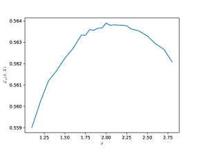
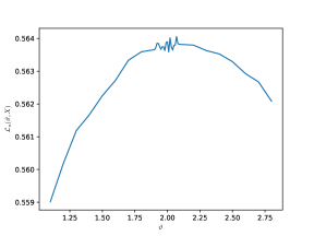
Figure 2. The contrast $\mathcal{L}_{n}\big{(}\vartheta,(X_{u},u\in\mathbb{T}_{n})\big{)}$ for $n=14$ and $B(x,\vartheta)\equiv 2$ with $\Delta\vartheta=0.05$ (left) and $\Delta\vartheta=0.01$ (right). We look at the results only for $\Delta\vartheta=0.05$ because for smaller values of the increment, the noise due to computational errors is too important compared to the different values of the contrast.

The results are displayed in Table 1. We recover the parameter in all four cases, with various accuracies. The most accurate value is obtained for $B_{1}$ with a small value of the parameter, i.e. $\vartheta=2$. We did not reach the optimal accuracy $|\mathbb{T}_{n}^{\star}|^{-1/2}\approx 6\times 10^{-3}$. One could presumably obtain a better accuracy by choosing a finer discretisation of $[0,1]\times[0,1]$ for the computation of the $\widehat{q}_{n}$. But this choice leads to an important increase of the computational time. The results in the case of a linear division rate are less accurate. Those results could also probably be improved using a cross-validation procedure for the choice of the bandwidth parameters $h,h_{1},h_{2}$.

$B$	$\vartheta$	Mean	Std Dev.	$\vartheta_{\min}$	$\vartheta_{\max}$	$\Delta\vartheta$
$B_{0}$	$2$	$1.9908$	$0.0845$	$1.8$	$2.2$	$0.05$
	$15$	$15.029$	$0.4763$	$14$	$16$	$0.25$
$B_{1}$	$2$	$2.1392$	$0.3485$	$1.375$	$3$	$0.125$
	$15$	$15.023$	$0.6425$	$13.75$	$16.5$	$0.25$

Table 1. Results for $B$ in $\mathcal{B}_{1}$ and $\mathcal{B}_{2}$. For each parametric class of functions $\mathcal{B}_{1}$ and $\mathcal{B}_{2}$, we display the results for $\vartheta=2$ and $\vartheta=15$. The third and fourth columns corresponds respectively to the mean value and the standard deviation of $\widehat{\vartheta}_{n}$, computed with $300$ different data sets of size $2^{n+1}-1=32767$. The fifth and sixth columns correspond to a $95\%$ confidence interval. The last column corresponds to the value of the step for the discretisation of $\Theta$, which limits the accuracy of the result.

5. Proofs

5.1. Proof of Proposition 5

We first prove (7). By (3), for any bounded $\psi:\mathcal{X}^{3}\rightarrow\mathbb{R}$ and $x\in\mathcal{X}$, we have

$$\mathcal{P}\psi(x) =\mathbb{E}\Big{[}\int_{0}^{1}\kappa(z)\int_{0}^{\infty}\psi\big{(}x,z\phi_{x}(t),(1-z)\phi_{x}(t)\big{)}B\big{(}\phi_{x}(t)\big{)}e^{-\int_{0}^{t}B(\phi_{x}(s))ds}dtdz\Big{]}$$

(14) $$=\int_{\mathbb{R}}\int_{0}^{1}\psi\big{(}x,y_{0},\tfrac{1-z}{z}y_{0}\big{)}B\big{(}y_{0}/z\big{)}\sigma(y_{0}/z)^{-2}\mathbb{E}\Big{[}\int_{0}^{\infty}e^{-\int_{0}^{t}B(\phi_{x}(s))ds}dL_{t}^{y_{0}/z}(\phi_{x})\Big{]}\frac{\kappa(z)}{z}dzdy_{0}$$

$$=\int_{\mathcal{D}}\psi\big{(}x,y_{0},y_{1}\big{)}\frac{\kappa\big{(}y_{0}/(y_{0}+y_{1})\big{)}}{y_{0}+y_{1}}\frac{B\left(y_{0}+y_{1}\right)}{\sigma(y_{0}+y_{1})^{2}}\mathbb{E}\Big{[}\int_{0}^{\infty}e^{-\int_{0}^{t}B(\phi_{x}(s))ds}dL_{t}^{y_{0}+y_{1}}(\phi_{x})\Big{]}dy_{0}dy_{1},$$

where we set $y_{1}=\frac{1-z}{z}y_{0}$ in order to obtain the last line and where $(L_{t}^{y}(\phi_{x}))_{t\geq 0}$ is the local time of $\phi_{x}$ at $y\in\mathcal{X}$. The integral is taken over the domain

$$\mathcal{D}=\big{\{}(y_{0},y_{1})\in\mathbb{R}^{2},\ \tfrac{\varepsilon}{1-\varepsilon}y_{0}\leq y_{1}\leq\tfrac{1-\varepsilon}{\varepsilon}y_{0}\big{\}}\subset\text{supp}\big{(}(y_{0},y_{1})\mapsto\kappa(y_{0}/(y_{0}+y_{1}))\big{)}$$

therefore the above integral is well defined and the representation (7) is proved. We turn to (8). From (5.1), we get

$$\mathcal{P}_{0}\varphi(x)=\int_{\mathbb{R}}\int_{0}^{1}\varphi(y_{0})B\big{(}y_{0}/z\big{)}\sigma(y_{0}/z)^{-2}\mathbb{E}\Big{[}\int_{0}^{\infty}e^{-\int_{0}^{t}B(\phi_{x}(s))ds}dL_{t}^{y_{0}/z}(\phi_{x})\Big{]}\frac{\kappa(z)}{z}dzdy_{0}$$

and

$$\mathcal{P}_{1}\varphi(x) =\int_{\mathbb{R}}\int_{0}^{1}\varphi\big{(}\tfrac{1-z}{z}y_{0}\big{)}B\big{(}y_{0}/z\big{)}\sigma(y_{0}/z)^{-2}\mathbb{E}\Big{[}\int_{0}^{\infty}e^{-\int_{0}^{t}B(\phi_{x}(s))ds}dL_{t}^{y_{0}/z}(\phi_{x})\Big{]}\frac{\kappa(z)}{z}dzdy_{0}$$

$$=\int_{\mathbb{R}}\int_{0}^{1}\varphi\big{(}y_{1}\big{)}B\big{(}y_{1}/\bar{z}\big{)}\sigma(y_{1}/\bar{z})^{-2}\mathbb{E}\Big{[}\int_{0}^{\infty}e^{-\int_{0}^{t}B(\phi_{x}(s))ds}dL_{t}^{y_{1}/\bar{z}}(\phi_{x})\Big{]}\frac{\kappa(1-\bar{z})}{\bar{z}}d\bar{z}dy_{1},$$

where the second equality is given by two successive changes of variables $y_{1}=\tfrac{1-z}{z}y_{0}$ and $\bar{z}=1-z$. Finally,

$$\mathcal{Q}\varphi(x) =\tfrac{1}{2}\big{(}\mathcal{P}_{0}\varphi(x)+\mathcal{P}_{1}\varphi(x)\big{)}$$

$$=\int_{\mathbb{R}}\int_{0}^{1}\varphi(y)B\big{(}y/z\big{)}\sigma(y/z)^{-2}\mathbb{E}\Big{[}\int_{0}^{\infty}e^{-\int_{0}^{t}B(\phi_{x}(s))ds}dL_{t}^{y/z}(\phi_{x})\Big{]}\frac{\widetilde{\kappa}(z)}{z}dzdy,$$

where $\widetilde{\kappa}(z)=\tfrac{1}{2}(\kappa(z)+\kappa(1-z))$. Since $\text{supp}(\kappa)\subset[\varepsilon,1-\varepsilon]$, the above integrals are well defined and (8) is established.

5.2. Proof of Proposition 6

The proof goes along a classical path: we establish a drift and a minorisation condition in Proposition 23 and 24 below, and then apply for instance Theorem 1.2. in [20], see also the references therein.

Proposition 23 (Drift condition).

Let $V(x)=x^{2}$. Work under Assumptions 2, 3 and 4. There exist explicitly computable $0<v_{1}=v_{1}(\varepsilon)<1$ and $v_{2}=v_{2}(\varepsilon,r_{1},r_{2},\sigma_{1},\sigma_{2},b_{1})>0$ such that

$$\mathcal{Q}V(x)\leq v_{1}V(x)+v_{2}.$$

Proposition 24 (Minorisation condition).

Work under Assumption 2, 3 and 4. For large enough $w>0$, there exists $\lambda\in(0,1)$ and a probability measure $\mu$ on $\mathcal{X}$ such that

$$\inf_{\{x,|x|\leq w\}}\mathcal{Q}(x,\mathcal{A})\geq\lambda\mu(\mathcal{A})$$

for every Borel set $\mathcal{A}\subset\mathcal{X}$.

Proof of Proposition 23.

Fix $x\in\mathcal{X}$ and let $m(\kappa)=\int_{0}^{1}z^{2}\widetilde{\kappa}(z)dz$. By Itô formula, we obtain the decomposition

$$\mathcal{Q}V(x)=\int_{0}^{1}\widetilde{\kappa}(z)\int_{0}^{\infty}\mathbb{E}\Big{[}z^{2}\phi_{x}(t)^{2}B\big{(}\phi_{x}(t)\big{)}e^{-\int_{0}^{t}B(\phi_{x}(s))ds}\Big{]}dtdz=m(\kappa)(I+II+III+IV),$$

where

$$I =x^{2}\int_{0}^{\infty}\mathbb{E}\Big{[}B\big{(}\phi_{x}(t)\big{)}e^{-\int_{0}^{t}B(\phi_{x}(s))ds}\Big{]}dt,$$

$$II =2\int_{0}^{\infty}\mathbb{E}\Big{[}\int_{0}^{t}\phi_{x}(u)r(\phi_{x}(u))du\,B\big{(}\phi_{x}(t)\big{)}e^{-\int_{0}^{t}B(\phi_{x}(s))ds}\Big{]}dt,$$

$$III =\int_{0}^{\infty}\mathbb{E}\Big{[}\int_{0}^{t}\sigma\big{(}\phi_{x}(u)\big{)}^{2}du\,B\big{(}\phi_{x}(t)\big{)}e^{-\int_{0}^{t}B(\phi_{x}(s))ds}\Big{]}dt,$$

$$IV =2\int_{0}^{\infty}\mathbb{E}\Big{[}\int_{0}^{t}\phi_{x}(u)\sigma\big{(}\phi_{x}(u)\big{)}dW_{u}\,B\big{(}\phi_{x}(t)\big{)}e^{-\int_{0}^{t}B(\phi_{x}(s))ds}\Big{]}dt.$$

First, note that $\int_{0}^{\infty}B(\phi_{x}(t))e^{-\int_{0}^{t}B(\phi_{x}(s))ds}dt=1$ holds since $B(\phi_{x}(t))\geq b_{1}>0$ by Assumption 3, therefore $I=x^{2}$ by Fubini’s theorem. We turn to $II$. By Fubini’s theorem again:

$$II =2\,\mathbb{E}\Big{[}\int_{0}^{\infty}\phi_{x}(u)r\big{(}\phi_{x}(u)\big{)}\big{(}\int_{u}^{\infty}B\big{(}\phi_{x}(t)\big{)}e^{-\int_{0}^{t}B(\phi_{x}(s))ds}dt\big{)}du\Big{]}$$

$$=2\,\mathbb{E}\Big{[}\int_{0}^{\infty}\phi_{x}(u)r\big{(}\phi_{x}(u)\big{)}e^{-\int_{0}^{u}B(\phi_{x}(s))ds}du\Big{]}$$

$$=2\int_{\mathbb{R}}zr(z)\sigma(z)^{-2}\mathbb{E}\Big{[}\int_{0}^{\infty}e^{-\int_{0}^{t}B(\phi_{x}(s))ds}dL_{t}^{z}(\phi_{x})\Big{]}dz.$$

where we used again that $e^{-\int_{0}^{\infty}B(\phi_{x}(s))ds}=0$ since $B(\phi_{x}(t))\geq b_{1}>0$ by Assumption 3 for the second equality and the occupation times formula for the last equality. By Assumption 2 we have $zr(z)<0$ for $|z|\geq r_{2}$, therefore:

$$II \leq 2\int_{-r_{2}}^{r_{2}}zr(z)\sigma(z)^{-2}\mathbb{E}\Big{[}\int_{0}^{\infty}e^{-\int_{0}^{t}B(\phi_{x}(s))ds}dL_{t}^{z}(\phi_{x})\Big{]}dz$$

$$\leq 2r_{1}r_{2}(1+r_{1})\sigma_{1}^{-2}\int_{-r_{2}}^{r_{2}}\mathbb{E}\Big{[}\int_{0}^{\infty}e^{-\int_{0}^{t}B(\phi_{x}(s))ds}dL_{t}^{z}(\phi_{x})\Big{]}dz$$

$$\leq 2r_{1}r_{2}(1+r_{1})\sigma_{1}^{-2}\int_{0}^{\infty}e^{-b_{1}t}\mathbb{P}\big{(}-r_{2}\leq\phi_{x}(t)\leq r_{2}\big{)}dt\leq 2r_{1}r_{2}(1+r_{1})\sigma_{1}^{-2}b_{1}^{-1}.$$

using successively Assumption 2, 3 and the occupation times formula. For the term $III$, by Fubini’s theorem, we have

$$III =\int_{0}^{\infty}\mathbb{E}\big{[}\sigma\big{(}\phi_{x}(u)\big{)}^{2}\int_{u}^{\infty}B\big{(}\phi_{x}(t)\big{)}e^{-\int_{0}^{t}B(\phi_{x}(s))ds}\Big{]}du$$

$$=\int_{0}^{\infty}\mathbb{E}\left[\sigma(\phi_{x}(u))^{2}e^{-\int_{0}^{u}B(\phi_{x}(s))ds}\right]du$$

and this last quantity is less than $\sigma^{2}_{2}\int_{0}^{\infty}e^{-b_{1}t}dt=\sigma^{2}_{2}b_{1}^{-1}$ by Assumption 2 and 3. Similarly for the term IV, we have

$$IV =2\,\mathbb{E}\Big{[}\int_{0}^{\infty}\sigma\big{(}\phi_{x}(u)\big{)}\int_{u}^{\infty}B\big{(}\phi_{x}(t)\big{)}e^{-\int_{0}^{t}B(\phi_{x}(s))ds}dtdW_{u}\Big{]}$$

$$=2\,\mathbb{E}\Big{[}\int_{0}^{\infty}\sigma\big{(}\phi_{x}(u)\big{)}e^{-\int_{0}^{u}B(\phi_{x}(s))ds}dW_{u}\Big{]}$$

and this last quantity vanishes. Putting the estimates for $I$, $II$, $III$ and $IV$ together, we conclude

$$\mathcal{Q}V(x)\leq m(\kappa)x^{2}+m(\kappa)(2r_{1}r_{2}(1+r_{1})\sigma_{1}^{-2}+\sigma_{2}^{2})b_{1}^{-1}.$$

Since $\text{supp}(\kappa)\subset[\varepsilon,1-\varepsilon]$, we have $m(\kappa)\leq(1-\varepsilon)^{2}<1$ and this completes the proof with $v_{1}=m(\kappa)$ and $v_{2}=m(\kappa)(2r_{1}r_{2}(1+r_{1})\sigma_{1}^{-2}+\sigma_{2}^{2})b_{1}^{-1}$.

∎

Proof of Proposition 24.

Step 1). Let $x\in[-w,w]$ and $\mathcal{A}\subset\mathcal{X}$ be a Borel set. Applying Assumption 3, introducing the event $\mathcal{W}(\phi_{x}(t))=\{2w\leq\phi_{x}(t)\leq 2w\sqrt{(1-\varepsilon)/\varepsilon)}\}$, applying Fubini’s theorem and a change of variable, we successively obtain

$$\mathcal{Q}(x,\mathcal{A}) =\int_{0}^{1}\widetilde{\kappa}(z)\int_{0}^{\infty}\mathbb{E}\Big{[}\mathbf{1}_{\left\{z\phi_{x}(t)\in\mathcal{A}\right\}}B\big{(}\phi_{x}(t)\big{)}e^{-\int_{0}^{t}B(\phi_{x}(s))ds}\Big{]}dtdz$$

$$\geq b_{1}\int_{0}^{1}\widetilde{\kappa}(z)\int_{0}^{\infty}\mathbb{E}\Big{[}{\bf 1}_{\mathcal{W}(\phi_{x}(t))}\mathbf{1}_{\left\{z\phi_{x}(t)\in\mathcal{A}\right\}}e^{-\int_{0}^{t}B\big{(}\phi_{x}(s)\big{)}ds}\Big{]}dtdz$$

$$=b_{1}\int_{0}^{\infty}\mathbb{E}\Big{[}{\bf 1}_{\mathcal{W}(\phi_{x}(t))}e^{-\int_{0}^{t}B\left(\phi_{x}(s)\right)ds}\int_{0}^{\phi_{x}(t)}\mathbf{1}_{\left\{y\in\mathcal{A}\right\}}\widetilde{\kappa}\big{(}y/\phi_{x}(t)\big{)}\phi_{x}(t)^{-1}dy\Big{]}dt.$$

Using again Fubini’s theorem, we get

$$\mathcal{Q}(x,\mathcal{A})\geq\int_{\mathbb{R}}\mathbf{1}_{\left\{y\in\mathcal{A}\right\}}f(x,y)dy,$$

with $f(x,y)=b_{1}\int_{0}^{\infty}\mathbb{E}\big{[}{\bf 1}_{\mathcal{W}(\phi_{x}(t))}\mathbf{1}_{\left\{y\leq\phi_{x}(t)\right\}}e^{-\int_{0}^{t}B\left(\phi_{x}(s)\right)ds}\widetilde{\kappa}\big{(}y/\phi_{x}(t)\big{)}\phi_{x}(t)^{-1}\big{]}dt.$

Step 2). We now prove that $f$ is bounded below independently of $x$. By Assumption 4, $\widetilde{\kappa}\big{(}y/\phi_{x}(t)\big{)}>\delta$ for all $y\in[\varepsilon\phi_{x}(t),(1-\varepsilon)\phi_{x}(t)]$ so that

$$f(x,y) \geq\delta b_{1}\int_{0}^{\infty}\mathbb{E}\Big{[}{\bf 1}_{\mathcal{W}(\phi_{x}(t))}\mathbf{1}_{\left\{\varepsilon\phi_{x}(t)\leq y\leq(1-\varepsilon)\phi_{x}(t)\right\}}e^{-\int_{0}^{t}B\left(\phi_{x}(s)\right)ds}\phi_{x}(t)^{-1}\Big{]}dt.$$

Next, as $\mathcal{W}(\phi_{x}(t))\bigcap\{\varepsilon\phi_{x}(t)\leq y\leq(1-\varepsilon)\phi_{x}(t)\}\supseteq\mathcal{W}(\phi_{x}(t))\bigcap\{2w\sqrt{\varepsilon(1-\varepsilon)}\leq y\leq 2w(1-\varepsilon)\}$, we get

$$f(x,y)\geq\frac{\delta b_{1}}{2w\sqrt{(1-\varepsilon)/\varepsilon}}\mathbf{1}_{\left\{2w\sqrt{\varepsilon(1-\varepsilon)}\leq y\leq 2w(1-\varepsilon)\right\}}h(x,y),$$

where $h(x,y)=\int_{0}^{\infty}\mathbb{E}\big{[}{\bf 1}_{\mathcal{W}(\phi_{x}(t))}e^{-\int_{0}^{t}B\left(\phi_{x}(s)\right)ds}\big{]}dt$. Let $\Delta=(1+\sqrt{(1-\varepsilon)/\varepsilon})w$ denote the mid-point of the interval $[2w,2w\sqrt{(1-\varepsilon)/\varepsilon}]$. Let also $T^{x}_{y}=\inf\left\{t>0,\phi_{x}(t)\geq y\right\}$ denote the exit time of the interval $(\inf\mathcal{X},y)$ by $(\phi_{x}(t))_{t\geq 0}$. It follows that

$$h(x,y) \geq\mathbb{E}\Big{[}\int_{T_{\Delta}^{x}}^{\infty}{\bf 1}_{\mathcal{W}(\phi_{x}(t))}e^{-\int_{0}^{t}B\left(\phi_{x}(s)\right)ds}dt\Big{]}$$

$$=\int_{0}^{\infty}\mathbb{E}\Big{[}\mathbf{1}_{\mathcal{W}(\phi_{x}(t+T_{\Delta}^{x}))}e^{-\int_{0}^{t+T_{\Delta}^{x}}B\left(\phi_{x}(s)\right)ds}\Big{]}dt$$

$$=\int_{0}^{\infty}\mathbb{E}\Big{[}\mathbf{1}_{\mathcal{W}(\phi_{x}(t+T_{\Delta}^{x}))}e^{-\int_{0}^{T_{\Delta}^{x}}B\left(\phi_{x}(s)\right)ds}e^{-\int_{0}^{t}B\left(\phi_{x}(s+T_{\Delta}^{x})\right)ds}\Big{]}dt$$

$$\geq\int_{0}^{\infty}\mathbb{E}\Big{[}\mathbf{1}_{\mathcal{W}(\phi_{x}(t+T_{\Delta}^{x}))}e^{-T_{\Delta}^{x}\left(b_{2}\Delta^{\gamma}+b_{1}\right)}e^{-\int_{0}^{t}B\left(\phi_{x}(s+T_{\Delta}^{x})\right)ds}\Big{]}dt,$$

by Assumption 3 and because $\phi_{x}(s)\leq\Delta$ for every $s\leq T_{\Delta}^{x}$. Applying the strong Markov property, we further obtain

(15) $$h(x,y)\geq\int_{0}^{\infty}\mathbb{E}\Big{[}\mathbf{1}_{\mathcal{W}(\phi_{\Delta}(t))}e^{-T_{\Delta}^{x}\left(b_{2}\Delta^{\gamma}+b_{1}\right)}e^{-\int_{0}^{t}B\left(\phi_{\Delta}(s)\right)ds}\Big{]}dt$$

since $\phi_{x}(T_{\Delta}^{x})=\Delta$ for $x\leq w<\Delta$. Introduce next $T_{\mathcal{W}}^{\Delta}=\inf\{t\geq 0,\ \phi_{\Delta}(t)\notin[2w,2w\sqrt{(1-\varepsilon)/\varepsilon}]\}$, i.e. the exit time of $[2w,2w\sqrt{(1-\varepsilon)/\varepsilon}]$ by $(\phi_{\Delta}(t))_{t\geq 0}$. By (15) and Assumption 3 again, it follows that

$$h(x,y) \geq\mathbb{E}\Big{[}\int_{0}^{T_{\mathcal{W}}^{\Delta}}\mathbf{1}_{\mathcal{W}(\phi_{\Delta}(t))}e^{-T_{\Delta}^{x}\left(b_{2}\Delta^{\gamma}+b_{1}\right)}e^{-\int_{0}^{t}\left(b_{2}|\phi_{x}(s)|^{\gamma}+b_{1}\right)ds}dt\Big{]}$$

$$\geq\mathbb{E}\left[\int_{0}^{T_{\mathcal{W}}^{\Delta}}\mathbf{1}_{\mathcal{W}(\phi_{\Delta}(t))}e^{-T_{\Delta}^{x}\left(b_{2}\Delta^{\gamma}+b_{1}\right)}e^{-tv_{3}}dt\right],$$

using that $\phi_{x}(t)\leq 2w\sqrt{(1-\varepsilon)/\varepsilon}$ for $t\leq T_{\mathcal{W}}^{\Delta}$ and where $v_{3}=b_{2}(2w\sqrt{(1-\varepsilon)/\varepsilon})^{\gamma}+b_{1}$. Since $\Delta>-w$, the event $\{T_{\Delta}^{x}\leq T_{\Delta}^{-w}\}$ holds almost-surely for every $x\in[-w,w]$ and therefore

(16) $$h(x,y)\geq\mathbb{E}\Big{[}\int_{0}^{T_{\mathcal{W}}^{\Delta}}e^{-T_{\Delta}^{-w}\left(b_{2}\Delta^{\gamma}+b_{1}\right)}e^{-tv_{3}}dt\Big{]}\geq v_{3}^{-1}\mathbb{E}\big{[}e^{-T_{\Delta}^{-w}\left(b_{2}\Delta^{\gamma}+b_{1}\right)}\big{]}\mathbb{E}\big{[}1-e^{-T_{\mathcal{W}}^{\Delta}v_{3}}\big{]}.$$

by the independence of $T_{\mathcal{W}}^{\Delta}$ and $T_{\Delta}^{-w}$. Furthermore, for every $a,x\in\mathcal{X}$ with $x<a$, we have

$$\mathbb{P}\left(T_{a}^{x}<\infty\right) =\lim_{u\rightarrow-\infty}\frac{s(u)-s(x)}{s(u)-s(a)},$$

where $s(x)=\int_{\inf\mathcal{X}}^{x}\exp(-2\int_{\inf\mathcal{X}}^{y}r(z)\sigma(z)^{-2}dz)dy$, is the scale function associated to $(\phi_{x}(t))_{t\geq 0}$. By the classical Feller classification of scalar diffusions (see e.g. Revuz and Yor [33]), we have the equivalence $\mathbb{P}\left(T_{a}^{x}<\infty\right)=0$ if only if $\int_{\inf\mathcal{X}}s(x)dx=0$ but that latter property contradicts Assumption 2. Therefore, there exist $w_{1},\delta_{1}>0$ such that $\mathbb{P}(T_{\Delta}^{-w}\leq w_{1})>\delta_{1}$. It follows that

(17) $$\mathbb{E}\big{[}e^{-T_{\Delta}^{-w}(b_{2}\Delta^{\gamma}+b_{1})}\big{]}\geq\mathbb{E}\big{[}e^{-w_{1}(b_{2}\Delta^{\gamma}+b_{1})}\mathbf{1}_{\{T_{\Delta}^{-w}\leq w_{1}\}}\big{]}\geq\delta_{1}e^{-w_{1}(b_{2}\Delta^{\gamma}+b_{1})}$$

and since $T_{\mathcal{W}}^{\Delta}>0$ almost surely, there exists $\delta_{2}>0$, independent of $x$, such that

(18) $$\mathbb{E}\big{[}1-e^{-T_{\mathcal{W}}^{\Delta}v_{3}}\big{]}>\delta_{2}.$$

Back to (16), putting together (17) and (18), we obtain

$$h(x,y)\geq v_{3}^{-1}\delta_{1}e^{-w_{1}(b_{2}\Delta^{\gamma}+b_{1})}\delta_{2}$$

and eventually

$$f(x,y)\geq\frac{\delta b_{1}\delta_{1}\delta_{2}}{2w\sqrt{(1-\varepsilon)/\varepsilon}v_{3}}\mathbf{1}_{\left\{2w\sqrt{\varepsilon(1-\varepsilon)}\leq y\leq 2w(1-\varepsilon)\right\}}e^{-w_{1}(b_{2}\Delta^{\gamma}+b_{1})}.$$

Step 3). Define the probability measure $\mu(dy)=f(y)dy$ on $\mathcal{X}$ by

$$f(y)=\frac{1}{2w\big{(}1-\varepsilon-\sqrt{\varepsilon(1-\varepsilon)}\big{)}}\mathbf{1}_{\left\{2w\sqrt{\varepsilon(1-\varepsilon)}\leq y\leq 2w(1-\varepsilon)\right\}},$$

and let $\lambda=(1-\varepsilon-\sqrt{\varepsilon(1-\varepsilon)})\frac{b_{1}\delta\delta_{1}\delta_{2}}{\sqrt{(1-\varepsilon)/\varepsilon}v_{3}}e^{-w_{1}\left(b_{2}\Delta^{\gamma}+b_{1}\right)}$. We may assume that $0<\lambda<1$ (the lower bound remains valid if we replace $\delta$ by $\delta^{\prime}<\delta$ for instance) and we thus have established

$$\mathcal{Q}(x,\mathcal{A})\geq\lambda\mu(\mathcal{A}),$$

for an arbitrary Borel set $\mathcal{A}\subset\mathcal{X}$. The proof of Proposition 24 is complete. ∎

5.3. Proof of Proposition 9

Preparations

We first state a useful estimate on the local time of $L_{t}^{y}(\phi_{x})$ as $t\rightarrow\infty$. Its proof is delayed until Appendix 6.2.

Lemma 25.

Work under Assumption 2. For every compact $\mathcal{K}\subset\mathcal{X}$ and for every $t\geq 0$, we have

$$\sup_{x\in\mathcal{X},y\in\mathcal{K}}\mathbb{E}\left[L_{t}^{y}\left(\phi_{x}\right)\right]\lesssim 1+t^{3/2},$$

up to a constant that only depends on $r_{1}$, $r_{2}$ and $\sigma_{2}$. In particular, for every $c>0$, the function

$$y\mapsto\int_{0}^{\infty}e^{-ct}\sup_{x\in\mathcal{X}}\mathbb{E}\left[L_{t}^{y}\left(\phi_{x}\right)\right]dt$$

is well-defined and locally bounded, uniformly over $\mathbb{Q}$.

Lemma 25 enables us to obtain estimates on the action of $\mathcal{P}$ and $\mathcal{Q}$ on functions $\psi:\mathcal{X}\times\mathcal{X}\rightarrow\mathbb{R}$ with nice behaviours that will prove essential for obtaining Proposition 9. We set

$$\mathcal{Q}\psi(x)=\int_{\mathcal{X}}\psi(x,y)q(x,y)dy,\;\;\mathcal{P}(\psi\otimes\psi)(x)=\int_{\mathcal{X}\times\mathcal{X}}\psi(x,y_{1})\psi(x,y_{2})p(x,y_{1},y_{2})dy_{1}dy_{2},$$

where $p(x,y_{1},y_{2})$ and $q(x,y)$ are given in Proposition 5.

Lemma 26.

Work under Assumptions 2, 3 and 4. Let $\psi:\mathcal{X}\times\mathcal{X}\rightarrow\mathbb{R}$ be bounded and such that $\psi_{\star}$ has compact support. There exists a constant $c_{\mathrm{supp}(\psi_{\star})}$ depending on $\mathrm{supp}(\psi_{\star})$ (and $\mathcal{Q}$) such that, for $i=0,1$:

(19) $$|\mathcal{P}_{i}\psi(x)|\leq c_{\mathrm{supp}(\psi_{\star})}\int_{\mathcal{X}}|\psi(x,y)|dy$$

and

$$|\mathcal{P}(\psi\otimes\psi)(x)|\leq c_{\mathrm{supp}(\psi_{\star})}\psi^{\star}(x)\int_{\mathcal{X}}|\psi(x,y)|dy.$$

Note in particular that (19) implies in turn the estimates

(20) $$|\mathcal{Q}\psi(x)|\leq c_{\mathrm{supp}(\psi_{\star})}\int_{\mathcal{X}}|\psi(x,y)|dy,$$

and, for $i=0,1$:

$$|\mathcal{Q}\mathcal{P}_{i}\psi(x)|\leq c_{\mathrm{supp}(\psi_{\star})}^{2}|\psi|_{1}\wedge c_{\mathrm{supp}(\psi_{\star})}\big{|}\int_{\mathcal{X}}\psi_{\star}(y)dy\big{|}\lesssim|\psi|_{\wedge 1}.$$

Proof.

By Assumption 3, we have

$$|\mathcal{P}_{0}\psi(x)| =\Big{|}\int_{0}^{1}\kappa(z)\int_{0}^{\infty}\mathbb{E}\big{[}\psi(x,z\phi_{x}(t))B\big{(}\phi_{x}(t)\big{)}e^{-\int_{0}^{t}B(\phi_{x}(s))ds}\big{]}dtdz\Big{|}$$

$$\leq\int_{0}^{1}\kappa(z)\int_{0}^{\infty}\mathbb{E}\big{[}\big{|}\psi(x,z\phi_{x}(t))\big{|}\big{(}b_{2}\left|\phi_{x}(t)\right|^{\gamma}+b_{1}\big{)}e^{-b_{1}t}\big{]}dtdz$$

$$\leq\int_{0}^{1}\kappa(z)\int_{0}^{\infty}\mathbb{E}\Big{[}\big{|}\psi(x,z\phi_{x}(t))\big{|}\big{(}b_{2}\left|\phi_{x}(t)\right|^{\gamma}+b_{1}\big{)}\int_{t}^{\infty}b_{1}e^{-b_{1}s}ds\Big{]}dtdz.$$

Next, by Fubini’s theorem and the occupation times formula, we derive

$$|\mathcal{P}_{0}\psi(x)| \leq\int_{0}^{1}\kappa(z)\int_{0}^{\infty}b_{1}e^{-b_{1}s}\int_{0}^{s}\mathbb{E}\big{[}|\psi(x,z\phi_{x}(t))|(b_{2}|\phi_{x}(t)|^{\gamma}+b_{1})\big{]}dtdsdz$$

$$\leq\int_{0}^{1}\kappa(z)\int_{0}^{\infty}b_{1}e^{-b_{1}s}\int_{\mathbb{R}}|\psi(x,zy)|(b_{2}|y|^{\gamma}+b_{1})\sigma(y)^{-2}\mathbb{E}[L_{s}^{y}(\phi_{x})]dydsdz$$

$$=\int_{0}^{1}\kappa(z)z^{-1}\int_{0}^{\infty}b_{1}e^{-b_{1}s}\int_{\mathbb{R}}|\psi(x,y)|(b_{2}|y/z|^{\gamma}+b_{1})\sigma(y/z)^{-2}\mathbb{E}[L_{s}^{y/z}(\phi_{x})]dydsdz$$

$$\leq c_{\mathrm{supp}(\psi_{\star})}\int_{\mathbb{R}}|\psi(x,y)|dy,$$

and (19) is proved for $i=0$ with

$$c_{\mathrm{supp}(\psi_{\star})}=\sup_{y\in\text{supp}(\psi_{\star}),x\in\mathcal{X},z\in[\varepsilon,1-\varepsilon]}b_{1}(b_{2}|y/z|^{\gamma}+b_{1})\sigma(y/z)^{-2}z^{-1}\int_{0}^{\infty}e^{-b_{1}s}\mathbb{E}[L_{s}^{y/z}(\phi_{x})]ds.$$

This last quantity is finite by Lemma 25. Following the same steps as for $\mathcal{P}_{1}$ we get (19) for $i=1$. For the second estimate, we have

$$|\mathcal{P}(\psi\otimes\psi)(x)| \leq\int_{0}^{1}\kappa(z)\int_{0}^{\infty}\mathbb{E}\big{[}\big{|}\psi\big{(}x,z\phi_{x}(t)\big{)}\psi\big{(}x,(1-z)\phi_{x}(t)\big{)}\big{|}B(\phi_{x}(t))e^{-\int_{0}^{t}B(\phi_{x}(s))ds}\big{]}dtdz$$

$$\leq\big{|}\mathcal{P}_{0}\psi(x)\big{|}\sup_{y}\big{|}\psi(x,y)\big{|}$$

and we conclude by applying (20). ∎

Completion of proof of Proposition 9

Without loss of generality, we may assume that $\nu(\mathcal{Q}\psi)=0$, the general case being obtained by considering the function $\psi(x,y)-\nu(\mathcal{Q}\psi)$. Of course, the compact support property is lost by adding a constant and one has to be careful when revisiting the estimates of Step 2) to Step 4) below. They exhibit additional error terms that all have the right order using Lemma 26 and the fact that $\mathcal{P}{\bf 1}=\mathcal{Q}{\bf 1}={\bf 1}$.

By (ii) of Definition 8 we may (and will) assume that for some $0\leq\varrho\leq 1$ and some positive constants $c_{1},c_{2}$ that do not depend on $n$, we have

$$c_{1}2^{\varrho m}\leq\big{|}\mathbb{G}_{m}\cap\mathbb{U}_{n}\big{|}\leq c_{2}2^{\varrho m}\;\;\text{for every}\;\;m=1,\ldots,n.$$

We first consider the case $\varrho>0$. The case $\varrho=0$ requires a slightly different method and will be handled in a second phase.

Step 1). We start with a standard preliminary decomposition, see for instance [8, 9], expanding the sum in $u\in\mathbb{U}_{n}^{\star}$.

We have

$$\mathbb{E}_{\mu}[\mathcal{M}_{\mathbb{U}_{n}}(\psi)^{2}] =|\mathbb{U}_{n}^{\star}|^{-2}\mathbb{E}_{\mu}\big{[}\big{(}\sum_{m=1}^{n}\sum_{u\in\mathbb{G}_{m}\cap\mathbb{U}_{n}}\psi(X_{u^{-}},X_{u})\big{)}^{2}\big{]}$$

$$\leq|\mathbb{U}_{n}^{\star}|^{-2}\Big{(}\sum_{m=1}^{n}\Big{(}\mathbb{E}_{\mu}\Big{[}\big{(}\sum_{u\in\mathbb{G}_{m}\cap\mathbb{U}_{n}}\psi(X_{u^{-}},X_{u})\big{)}^{2}\Big{]}\Big{)}^{1/2}\Big{)}^{2}$$

by triangle inequality. Thus Proposition 9 amounts to control

$$\mathbb{E}_{\mu}\big{[}\big{(}\sum_{u\in\mathbb{G}_{m}\cap\mathbb{U}_{n}}\psi(X_{u^{-}},X_{u})\big{)}^{2}\big{]}=I_{m}+II_{m},$$

with

$$I_{m} =\mathbb{E}_{\mu}\big{[}\sum_{u\in\mathbb{G}_{m}\cap\mathbb{U}_{n}}\psi(X_{u^{-}},X_{u})^{2}\big{]},$$

$$II_{m} =\mathbb{E}_{\mu}\big{[}\sum_{u,v\in\mathbb{G}_{m}\cap\mathbb{U}_{n},u\neq v}\psi(X_{u^{-}},X_{u})\psi(X_{v^{-}},X_{v})\big{]},$$

and the convention $\sum_{\emptyset}=0$.

Step 2). The control of the term $I_{m}$ is straightforward: by Lemma 26 we have

$$I_{1} =|\mathbb{G}_{1}\cap\mathbb{U}_{1}|\,\mu(\mathcal{Q}\psi^{2})\leq c_{2}2^{\varrho}c_{\mathrm{supp}(\psi_{\star})}\int_{\mathcal{X}\times\mathcal{X}}\psi(x,y)^{2}\mu(dx)dy\;\;\text{for}\;\;m=1,$$

$$I_{m} =|\mathbb{G}_{m}\cap\mathbb{U}_{m}|\,\mu(\mathcal{Q}^{m}\psi^{2})\leq c_{2}2^{\varrho m}(c_{\mathrm{supp}(\psi_{\star})}^{2}|\psi^{2}|_{1}\wedge c_{\mathrm{supp}(\psi_{\star})}|\psi_{\star}^{2}|_{1})\;\;\text{for}\;\;m\geq 2,$$

therefore $I_{m}\lesssim 2^{\varrho m}|\psi^{2}|_{\mu}$ holds for every $m\geq 1$. In the case $\nu(\mathcal{Q}\psi)\neq 0$, we replace $|\psi^{2}|_{\mu}$ by $|\psi^{2}|_{\mu+\nu}$.

Step 3). We further decompose the main term $II_{m}=III_{m}+IV_{m}$, having

$$III_{m} =\mathbb{E}_{\mu}\big{[}\sum_{w\in\mathbb{G}_{m-1}\cap\mathbb{U}_{n},(w0,w1)\in\mathbb{U}_{n}^{2}}\psi(X_{w},X_{w0})\psi(X_{w},X_{w1})\big{]},$$

$$IV_{m} =\mathbb{E}_{\mu}\big{[}\sum_{u,v\in\mathbb{G}_{m-1}\cap\mathbb{U}_{n},u\neq v}\hskip 5.69054pt\sum_{ui,vj\in\mathbb{U}_{n},i,j=0,1}\psi(X_{u},X_{ui})\psi(X_{v},X_{vj})\big{]}.$$

The control of $III_{m}$ is straightforward:

$$III_{m}=\mathbb{E}_{\mu}\big{[}\sum_{w\in\mathbb{G}_{m-1}\cap\mathbb{U}_{n}}\mathcal{P}(\psi\otimes\psi)(X_{w})\big{]}=|\mathbb{G}_{m-1}\cap\mathbb{U}_{n}|\,\mu\big{(}\mathcal{Q}^{m-1}\mathcal{P}(\psi\otimes\psi)\big{)}.$$

In the same way as for the term $I_{m}$, by Lemma 26, one readily checks that $|III_{m}|\lesssim 2^{\varrho(m-1)}|\psi^{\star}\psi|_{\mu}$.

Step 4). We now turn to the main term $IV_{m}$. Writing here $u\wedge v$ for the most common recent ancestor of $u$ and $v$, conditioning w.r.t. $\mathcal{F}_{|u\wedge v|+1}$ and using the conditional independence of $(X_{u},X_{ui})$ and $(X_{v},X_{vj})$ given $\mathcal{F}_{|u\wedge v|+1}$ thanks to the BMC property (3), we successively obtain

$$IV_{m} =\mathbb{E}_{\mu}\Big{[}\sum_{u,v\in\mathbb{G}_{m-1}\cap\mathbb{U}_{n},u\neq v}\hskip 5.69054pt\sum_{ui,vj\in\mathbb{U}_{n},i,j=0,1}\mathbb{E}_{\mu}\left[\psi(X_{u},X_{ui})\psi(X_{v},X_{vj})\big{|}\mathcal{F}_{|u\wedge v|+1}\right]\Big{]}$$

$$=\mathbb{E}_{\mu}\Big{[}\sum_{u,v\in\mathbb{G}_{m-1}\cap\mathbb{U}_{n},u\neq v}\hskip 5.69054pt\sum_{ui,vj\in\mathbb{U}_{n},i,j=0,1}\mathbb{E}_{\mu}\left[\psi(X_{u},X_{ui})\big{|}\mathcal{F}_{|u\wedge v|+1}\right]\mathbb{E}_{\mu}\left[\psi(X_{v},X_{vj})\big{|}\mathcal{F}_{|u\wedge v|+1}\right]\Big{]}$$

$$=\mathbb{E}_{\mu}\Big{[}\sum_{u,v\in\mathbb{G}_{m-1}\cap\mathbb{U}_{n},u\neq v}\hskip 5.69054pt\sum_{ui,vj\in\mathbb{U}_{n},i,j=0,1}\mathbb{E}_{\mu}\left[\mathcal{P}_{i}\psi(X_{u})\big{|}\mathcal{F}_{|u\wedge v|+1}\right]\mathbb{E}_{\mu}\left[\mathcal{P}_{j}\psi(X_{v})\big{|}\mathcal{F}_{|u\wedge v|+1}\right]\Big{]}$$

$$=\mathbb{E}_{\mu}\Big{[}\sum_{u,v\in\mathbb{G}_{m-1}\cap\mathbb{U}_{n},u\neq v}\hskip 5.69054pt\sum_{ui,vj\in\mathbb{U}_{n},i,j=0,1}\mathcal{Q}^{m-2-|u\wedge v|}\mathcal{P}_{i}\psi(X_{u^{*}})\mathcal{Q}^{m-2-|u\wedge v|}\mathcal{P}_{j}\psi(X_{v^{*}})\Big{]},$$

where $u^{*}$ (respectively $v^{*}$) is the descendant of $u\wedge v$ which is an ancestor of $u$ (respectively $v$). Conditioning further w.r.t. $\mathcal{F}_{\left|u\wedge v\right|}$ we obtain

$$IV_{m} =\mathbb{E}_{\mu}\Big{[}\sum_{u,v\in\mathbb{G}_{m-1}\cap\mathbb{U}_{n},u\neq v}\hskip 5.69054pt\sum_{ui,vj\in\mathbb{U}_{n},i,j=0,1}\mathcal{P}\big{(}\mathcal{Q}^{m-2-|u\wedge v|}\mathcal{P}_{i}\psi\otimes\mathcal{Q}^{m-2-|u\wedge v|}\mathcal{P}_{j}\psi\big{)}(X_{u\wedge v})\Big{]}$$

$$=\sum_{u,v\in\mathbb{G}_{m-1}\cap\mathbb{U}_{n},u\neq v}\hskip 5.69054pt\sum_{ui,vj\in\mathbb{U}_{n},i,j=0,1}\mu\big{(}\mathcal{Q}^{|u\wedge v|}\mathcal{P}(\mathcal{Q}^{m-2-|u\wedge v|}\mathcal{P}_{i}\psi\otimes\mathcal{Q}^{m-2-|u\wedge v|}\mathcal{P}_{j}\psi)\big{)}$$

$$=\sum_{l=1}^{m-1}\sum_{u,v\in\mathbb{G}_{m-1}\cap\mathbb{U}_{n},|u\wedge v|=m-l-1}\hskip 5.69054pt\sum_{ui,vj\in\mathbb{U}_{n},i,j=0,1}\,\mu\big{(}\mathcal{Q}^{m-l-1}\mathcal{P}(\mathcal{Q}^{l-1}\mathcal{P}_{i}\psi\otimes\mathcal{Q}^{l-1}\mathcal{P}_{j}\psi)\big{)},$$

obtaining the last term by rearranging the sum $u,v\in\mathbb{G}_{m-1}$ that expands over indexes $|u|-|u\wedge v|=m-1-|u\wedge v|$ that vary from $1$ to $m-1$. By Lemma 26 and Proposition 6 one obtains the following estimates for all $i,j=0,1$:

$$|\mu\left(\mathcal{Q}^{m-2}\mathcal{P}\left(\mathcal{P}_{i}\psi\otimes\mathcal{P}_{j}\psi\right)\right)|\lesssim|\psi_{\star}|_{1}|\psi|_{\wedge 1}\;\;\text{for}\;\;l=1,$$

and for $l\geq 2$:

$$|\mu\big{(}\mathcal{Q}^{m-l-1}\mathcal{P}(\mathcal{Q}^{l-1}\mathcal{P}_{i}\psi\otimes\mathcal{Q}^{l-1}\mathcal{P}_{j}\psi)\big{)}|\lesssim|\psi|_{\wedge 1}^{2}\,\wedge\,\rho^{2(l-1)}|\psi_{\star}|_{1}^{2}\,\mu\big{(}\mathcal{Q}^{m-l-1}\mathcal{P}((1+V)\otimes(1+V))\big{)}.$$

In the case $\nu(\mathcal{Q}\psi)\neq 0$, we replace $|\psi|_{\wedge 1}$ by $|\psi|_{\nu}$. We claim that

(21) $$\mu\big{(}\mathcal{Q}^{m-l-1}\mathcal{P}((1+V)\otimes(1+V))\big{)}\lesssim 1+\mu(V^{2})$$

and postpone the proof of (21) to Step 6 below. Notice also that for $l=1,\ldots,m-1$,

$$\big{|}\{u\neq v\in\mathbb{G}_{m-1}\cap\mathbb{U}_{n},|u\wedge v|=m-l-1\}\big{|}\lesssim 2^{\varrho m}\times 2^{l},$$

where $2^{\varrho m}$ is an upper bound for the number of choices for $u$ (the first descendant in generation ${m-1}$ of the ancestor from generation $m-l-1$) and $2^{l}$ is the (order of the) number of choices of $v$ (the second descendant, satisfying $u\wedge v\in\mathbb{G}_{m-l-1}$) in the worst case where there is a full subtree with $l$ generations. It follows that for any $p\geq 1$:

$$|IV_{m}| \lesssim 2^{\varrho m}|\psi_{\star}|_{1}|\psi|_{\wedge 1}+2^{\varrho m}\sum_{l=1}^{\infty}2^{l}\big{(}|\psi|_{\wedge 1}^{2}\,\wedge\,\rho^{2(l-1)}|\psi_{\star}|_{1}^{2}\big{(}1+\mu(V^{2})\big{)}\big{)}$$

$$\leq 2^{\varrho m}|\psi_{\star}|_{1}|\psi|_{\wedge 1}+2^{\varrho m}\Big{(}|\psi|_{\wedge 1}^{2}\sum_{l=1}^{p}2^{l}+|\psi_{\star}|_{1}^{2}\big{(}1+\mu(V^{2})\big{)}\sum_{l=p+1}^{\infty}2^{-l}(2\rho)^{2l}\Big{)}$$

$$\lesssim 2^{\varrho m}|\psi_{\star}|_{1}|\psi|_{\wedge 1}+2^{\varrho m}\Big{(}|\psi|_{\wedge 1}^{2}2^{p}+|\psi_{\star}|_{1}^{2}\big{(}1+\mu(V^{2})\big{)}2^{-p}\Big{)}$$

where we crucially used the fact that $\rho\leq 2^{-1}$. Then, taking the infimum over all $p\geq 1$, we get

$$|IV_{m}|\lesssim 2^{\varrho m}|\psi_{\star}|_{1}|\psi|_{\wedge 1}+2^{\varrho m}|\psi_{\star}|_{1}|\psi|_{\wedge 1}\big{(}1+\mu(V^{2})\big{)}\inf_{p\geq 1}\Big{(}\frac{|\psi|_{\wedge 1}}{|\psi_{\star}|_{1}}2^{p}+\frac{|\psi_{\star}|_{1}}{|\psi|_{\wedge 1}}2^{-p}\Big{)}.$$

As $|\psi|_{\wedge 1}\leq|\psi_{\star}|_{1}$, we get that $\inf_{p\geq 1}\Big{(}\frac{|\psi|_{\wedge 1}}{|\psi_{\star}|_{1}}2^{p}+\frac{|\psi_{\star}|_{1}}{|\psi|_{\wedge 1}}2^{-p}\Big{)}\lesssim 1$ and

$$|IV_{m}|\lesssim 2^{\rho m}\big{(}1+\mu(V^{2})\big{)}|\psi_{\star}|_{1}|\psi|_{\wedge 1}.$$

Step 5). Putting together the estimates obtained for $I_{m}$ in Step 2, $III_{m}$ in Step 3 and $IV_{m}$ in Step 4, and recalling $II_{m}=III_{m}+IV_{m}$ we eventually derive:

$$\mathbb{E}_{\mu}\big{[}\big{(}\sum_{u\in\mathbb{G}_{m}\cap\mathbb{U}_{n}}\psi(X_{u^{-}},X_{u})\big{)}^{2}\big{]}\lesssim 2^{\varrho m}\big{(}|\psi^{2}|_{\mu}+|\psi^{\star}\psi|_{\mu}+\big{(}1+\mu(V^{2})\big{)}|\psi_{\star}|_{1}|\psi|_{\wedge 1}\big{)}.$$

In the case $\nu(\mathcal{Q}\psi)\neq 0$, we replace $|\psi^{2}|_{\mu}$ by $|\psi^{2}|_{\mu+\nu}$ and $|\psi|_{\wedge 1}$ by $|\psi|_{\nu}$ as follows from Step 2 and 4. Taking square root, summing in $1\leq m\leq n$, taking square again and normalising by $|\mathbb{U}_{n}^{\star}|^{-2}$ which is of order $2^{-2\varrho n}$, we obtain Proposition 9.

Step 6). It remains to establish (21). We only sketch the argument which is similar to the proof of Proposition 23. First, one obtains

$$\mathcal{P}((1+V)\otimes(1+V))\lesssim 1+\mathcal{Q}V(x)+\mathcal{Q}V^{2}(x),$$

and it follows that

$$\mu(\mathcal{Q}^{m-l-1}\mathcal{P}\big{(}(1+V)\otimes(1+V))\big{)} \lesssim 1+\mu(\mathcal{Q}^{m-l}V)+\mu(\mathcal{Q}^{m-l}V^{2})$$

$$\lesssim 1+\mu(V)+\mu(\mathcal{Q}^{m-l}V^{2})$$

by Proposition 23. Applying Itô’s formula and using Assumptions 2 and 3 on can check that

$$\mathcal{Q}V^{2}(x)\lesssim 1+V(x)^{2}+\mathcal{Q}V(x)\lesssim 1+V(x)^{2}$$

by Proposition 23 again. We obtain (21) by integrating w.r.t. $\mu$. Finally the case $\varrho=0$ has to be treated separately mainly for notational reason, the proof following the same line as in the case $\varrho>0$. We delay it until Appendix 6.3.

5.4. Proof of Theorem 12

Preparations

We first establish local estimates on the invariant density $\nu$.

Lemma 27.

Work under Assumptions 2, 3 and 4. Let $\mathcal{Q}\in\mathbb{Q}$ and let $\nu$ be the associated invariant density of Proposition 6. Let $x_{0}\in\mathcal{X}$. There exist positive constants $c_{i}=c_{i}(x_{0},\mathcal{Q})$ and a bounded neighbourhood $\mathcal{V}_{x_{0}}$ with non-empty interior such that

$$0<c_{1}\leq\inf_{x\in\mathcal{V}_{x_{0}}}\nu(x)\leq\sup_{x\in\mathcal{V}_{x_{0}}}\nu(x)\leq c_{2}.$$

Moreover, $0<\inf_{\mathcal{Q}\in\mathbb{Q}}c_{1}(x_{0},\mathcal{Q})\leq\sup_{\mathcal{Q}\in\mathbb{Q}}c_{2}(x_{0},\mathcal{Q})<\infty.$

Proof.

Let $\mathcal{V}_{x_{0}}=[a,b]\subset\mathcal{X}$ be a bounded neighbourhood of $x_{0}$ and

$$\mathcal{V}_{x_{0}}^{\varepsilon}=\big{[}a/(1-\varepsilon)\wedge a/\varepsilon,\ b/\varepsilon\vee b/(1-\varepsilon)\big{]}.$$

Let $x\in\mathcal{V}_{x_{0}}$. By Proposition 5, using Assumptions 2 and 3, we obtain

$$\nu(x) =\int_{\mathcal{X}}\nu(y)q(y,x)dy$$

$$=\int_{\mathcal{X}}\nu(y)\int_{0}^{1}\frac{\widetilde{\kappa}(z)}{z}B(x/z)\sigma(x/z)^{-2}\mathbb{E}\Big{[}\int_{0}^{\infty}e^{-\int_{0}^{t}B(\phi_{y}(s))ds}dL_{t}^{x/z}(\phi_{y})\Big{]}dzdy$$

$$\leq\int_{\mathcal{X}}\nu(y)\int_{0}^{1}(b_{2}|x/z|^{\gamma}+b_{1})\frac{\widetilde{\kappa}(z)}{z}\sigma_{1}^{-2}\mathbb{E}\Big{[}\int_{0}^{\infty}e^{-b_{1}t}dL_{t}^{x/z}(\phi_{y})\Big{]}dzdy.$$

Noticing that for all $z\in[\varepsilon,1-\varepsilon]$ and $x\in\mathcal{V}_{x_{0}}$, $x/z\in\mathcal{V}_{x_{0}}^{\varepsilon}$ and using Assumption 4, we get

$$\nu(x) \leq(b_{2}|x|^{\gamma}+b_{1})\varepsilon^{-(1+\gamma)}\sigma_{1}^{-2}\int_{\mathcal{X}}\nu(y)\sup_{x\in\mathcal{V}_{x_{0}}^{\varepsilon}}\mathbb{E}\Big{[}\int_{0}^{\infty}e^{-b_{1}t}dL_{t}^{x}(\phi_{y})\Big{]}dy$$

$$=(b_{2}|x|^{\gamma}+b_{1})\varepsilon^{-(1+\gamma)}\sigma_{1}^{-2}b_{1}\int_{\mathcal{X}}\nu(y)\int_{0}^{\infty}e^{-b_{1}t}\sup_{x\in\mathcal{V}_{x_{0}}^{\varepsilon}}\mathbb{E}\big{[}L_{t}^{x}(\phi_{y})\big{]}dtdy,$$

where the last equality comes from the integration by parts formula, see Appendix 6.4 for a detailed version. By Lemma 25, we have $\sup_{x\in\mathcal{V}_{x_{0}}^{\varepsilon}}\mathbb{E}\big{[}L_{t}^{x}\left(\phi_{y}\right)\big{]}\lesssim 1+t^{3/2}$ uniformly over $\mathbb{Q}$ and the first part of the lemma follows. For the second part of the lemma, we have

$$\nu(x) \geq b_{1}\sigma_{2}^{-2}\int_{\mathcal{X}}\nu(y)\inf_{x\in\mathcal{V}_{x_{0}}^{\varepsilon}}\mathbb{E}\Big{[}\int_{0}^{\infty}e^{-b_{2}\int_{0}^{t}|\phi_{y}(s)|^{\gamma}ds-b_{1}t}dL_{t}^{x}(\phi_{y})\Big{]}dy$$

$$\geq b_{1}\sigma_{2}^{-2}\int_{[-N,N]\cap\mathcal{X}}\nu(y)\inf_{x\in\mathcal{V}_{x_{0}}^{\varepsilon}}\mathbb{E}\Big{[}\int_{0}^{T}e^{-(b_{2}M^{\gamma}+b_{1})t}dL_{t}^{x}(\phi_{y}){\bf 1}_{\{\sup_{t\leq T}|\phi_{y}(t)|\leq M\}}\Big{]}dy$$

$$\geq b_{1}\sigma_{2}^{-2}e^{-(b_{2}M^{\gamma}+b_{1})T}\int_{[-N,N]\cap\mathcal{X}}\nu(y)\inf_{x\in\mathcal{V}_{x_{0}}^{\varepsilon}}\mathbb{E}\big{[}L_{T}^{x}(\phi_{y}){\bf 1}_{\{\sup_{t\leq T}|\phi_{y}(t)|\leq M\}}\big{]}dy$$

for arbitrary constants $M,N,T>0$. Since $\mathbb{E}\big{[}L_{T}^{x}(\phi_{y}){\bf 1}_{\{\sup_{t\leq T}|\phi_{y}(t)|\leq M\}}\big{]}\uparrow\mathbb{E}\big{[}L_{T}^{x}(\phi_{y})\big{]}$ uniformly in $(x,y)\in\mathcal{V}_{x_{0}}\times[-N,N]$ as $M$ grows, pick $M$ large enough so that for every $y\in[-N,N]\cap\mathcal{X}$, we have

$$\inf_{x\in\mathcal{V}_{x_{0}}^{\varepsilon}}\mathbb{E}\big{[}L_{T}^{x}(\phi_{y}){\bf 1}_{\{\sup_{t\leq T}|\phi_{y}(t)|\leq M\}}\big{]}\geq\tfrac{1}{2}\inf_{x\in\mathcal{V}_{x_{0}}^{\varepsilon}}\mathbb{E}\big{[}L_{T}^{x}(\phi_{y})\big{]}.$$

Next, we use the fact that Assumption 2 implies that the law of the random variable $\phi_{y}(t)$ admits a density $\rho_{t}(y,x)$ w.r.t. the Lebesgue measure and that this density is bounded away from zero on compact sets in $(y,x)$, see for instance [13, 18]. In turn $\mathbb{E}\big{[}L_{T}^{x}(\phi_{y})\big{]}=\int_{0}^{T}\rho_{t}(y,x)dt\geq\tau_{T}>0$ for some $\tau_{T}$ depending also on $M$ and $N$ and we infer

$$\nu(x)\geq\frac{\tau_{T}}{2}b_{1}\sigma_{2}^{-2}e^{-(b_{2}M^{\gamma}+b_{1})T}\int_{[-N,N]\cap\mathcal{X}}\nu(y)dy$$

and we obtain the result by taking $N$ sufficiently large. The proof is complete. ∎

Completion of proof of Theorem 12

Step 1). Write $\widehat{\nu}_{n}(y_{0})-\nu(y_{0})=I+II$, with

$$I=\frac{1}{|\mathbb{U}_{n}|}\sum_{u\in\mathbb{U}_{n}}G_{h}(y_{0}-X_{u})-\nu(\mathcal{Q}G_{h}(y_{0}-\cdot))\;\;\text{and}\;\;II=G_{h}\star\nu(y_{0})-\nu(y_{0}).$$

We plan to apply Proposition 9 to $I$ with $\psi(x,y)=\varphi(y)=G_{h}(y_{0}-y)$. By Lemma 27, $\nu$ is locally bounded and we check that

$$|\psi^{2}|_{\mu+\nu}\lesssim\int_{\mathcal{X}}|G_{h}(y_{0}-y)^{2}|dy\lesssim h^{-1}\int_{\mathbb{R}}G(y)^{2}dy\lesssim h^{-1},$$

$$|\psi^{\star}\psi|_{\mu}\lesssim\sup_{y}|G_{h}(y)|\int_{\mathbb{R}}|G_{h}(y_{0}-y)|dy\lesssim h^{-1},$$

and

$$|\psi_{\star}|_{1}|\psi|_{\wedge 1}\lesssim\Big{(}\int_{\mathcal{X}}|G_{h}(y_{0}-y)|dy\Big{)}^{2}\lesssim 1.$$

Therefore, by Proposition 9, we have $\mathbb{E}_{\mu}[I^{2}]\lesssim|\mathbb{U}_{n}|^{-1}h^{-1}$ and this term is of order $|\mathbb{U}_{n}|^{-2\beta/(2\beta+1)}$ from the choice of $h$. For the term $II$, Lemma 27 and the representation $\nu(x)=\int_{\mathcal{X}}\nu(y)q(y,x)dy$ show that $\nu\in\mathcal{H}^{\beta}(y_{0})$ as soon as $q\in\mathcal{H}^{\alpha,\beta}(x_{0},y_{0})$. Then, by classical kernel approximation (see e.g. Chapter 1 of the book by Tsybakov [36]) we have that $II^{2}\lesssim h^{2\beta}$ since the order $k$ of the kernel $G$ satisfies $k>\beta$, and thus $II^{2}$ has the same order as $I^{2}$ from the choice of $h$.

Step 2). For the estimation of $q(x_{0},y_{0})$, write

$$\widehat{q}_{n}(x_{0},y_{0})-q(x_{0},y_{0})=I+II,$$

with

$$I=\frac{\mathcal{M}_{\mathbb{U}_{n}}\big{(}G_{h_{1},h_{2}}^{\otimes 2}(x_{0}-\cdot,y_{0}-\cdot)\big{)}-\nu(x_{0})q(x_{0},y_{0})}{\mathcal{M}_{\mathbb{U}_{n}}\big{(}G_{h}(x_{0}-\cdot)\big{)}\vee\varpi_{n}},$$

and

$$II=\frac{q(x_{0},y_{0})\big{(}\nu(x_{0})-\mathcal{M}_{\mathbb{U}_{n}}\big{(}G_{h}(x_{0}-\cdot)\big{)}\vee\varpi_{n}\big{)}}{\mathcal{M}_{\mathbb{U}_{n}}\big{(}G_{h}(x_{0}-\cdot)\big{)}\vee\varpi_{n}}.$$

We have $\big{|}I\big{|}\leq III+IV,$ with

$$III=\varpi_{n}^{-1}\big{|}\mathcal{M}_{\mathbb{U}_{n}}\big{(}G_{h_{1},h_{2}}^{\otimes 2}(x_{0}-\cdot,y_{0}-\cdot)\big{)}-G_{h_{1},h_{2}}^{\otimes 2}\star\nu(x_{0})q(x_{0},y_{0})\big{|}$$

and

$$IV=\varpi_{n}^{-1}\big{|}G_{h_{1},h_{2}}^{\otimes 2}\star\nu(x_{0})q(x_{0},y_{0})-\nu(x_{0})q(x_{0},y_{0})\big{|}.$$

We plan to apply Proposition 9 to bound $III$ with $\psi(x,y)=G_{h_{1},h_{2}}(x_{0}-x,y_{0}-y)$. Using Lemma 27 and the fact that $\mu$ is absolutely continuous, we have $|\psi|_{\mu+\nu}\lesssim|\psi|_{1}$. It readily follows that

$$|\psi^{2}|_{\mu+\nu} \lesssim|G_{h_{1}}(x_{0}-\cdot)^{2}|_{1}|G_{h_{2}}(y_{0}-\cdot)^{2}|_{1}\lesssim h_{1}^{-1}h_{2}^{-1},$$

$$|\psi^{\star}\psi|_{\mu}\;\, \lesssim|G_{h_{1}}(x_{0}-\cdot)\sup_{y}|G_{h_{2}}(y_{0}-y)|G_{h_{1}}(x_{0}-\cdot)G_{h_{2}}(y_{0}-\cdot)|_{1}$$

$$=|G_{h_{1}}(x_{0}-\cdot)^{2}|_{1}\sup_{y}|G_{h_{2}}(y_{0}-y)||G_{h_{2}}(y_{0}-\cdot)|_{1}\lesssim h_{1}^{-1}h_{2}^{-1},$$

and

$$|\psi_{\star}|_{1}|\psi|_{1}\lesssim\sup_{x}|G_{h_{1}}(x_{0}-x)||G_{h_{2}}(y_{0}-\cdot)|_{1}^{2}|G_{h_{1}}(x_{0}-\cdot)|_{1}\lesssim h_{1}^{-1}.$$

We conclude

$$\mathbb{E}_{\mu}\big{[}III^{2}\big{]}\lesssim\varpi_{n}^{-2}|\mathbb{U}_{n}|^{-1}h_{1}^{-1}h_{2}^{-1},$$

and this term has order $\varpi_{n}^{-2}|\mathbb{U}_{n}|^{-2s(\alpha,\beta)/(2s(\alpha,\beta)+1)}$ from the choice of $h_{1}$ and $h_{2}$. By kernel approximation and the fact that $G$ has order $k>\max\{\alpha,\beta\}$, noting that $(x,y)\mapsto\mu(x)q(x,y)\in\mathcal{H}^{\alpha\wedge\beta,\beta}$, we have

$$|IV|\lesssim h_{1}^{\alpha\wedge\beta}+h_{2}^{\beta}\lesssim\varpi_{n}^{-1}|\mathbb{U}_{n}|^{-s(\alpha,\beta)/(2s(\alpha,\beta)+1)}$$

from the choice of $h_{1},h_{2}$.

We turn to the term $II$. We plan to use

$$\big{(}\nu(x_{0})-\mathcal{M}_{\mathbb{U}_{n}}\big{(}G_{h}(x_{0}-\cdot)\big{)}\vee\varpi_{n}\big{)}^{2}\lesssim\big{(}\nu(x_{0})-\mathcal{M}_{\mathbb{U}_{n}}\big{(}G_{h}(x_{0}-\cdot)\big{)}\big{)}^{2}+{\bf 1}_{\big{\{}\mathcal{M}_{\mathbb{U}_{n}}(G_{h}(x_{0}-\cdot))<\varpi_{n}\big{\}}}.$$

Pick $n$ large enough so that $0<\varpi_{n}\leq\tau(x_{0})=\tfrac{1}{2}\inf_{\mathcal{Q}\in\mathbb{Q},x\in\mathcal{V}_{x_{0}}}\nu(x)$, a choice which is possible by Lemma 27. Since $\{\mathcal{M}_{\mathbb{U}_{n}}(G_{h}(x_{0})-\cdot)<\varpi_{n}\}\subset\{\mathcal{M}_{\mathbb{U}_{n}}(G_{h}(x_{0}-\cdot))-\nu(x_{0})<-\tau(x_{0})\}$, we further infer

$$\mathbb{E}_{\mu}\big{[}\big{(}\nu(x_{0})-\mathcal{M}_{\mathbb{U}_{n}}\big{(}G_{h}(x_{0}-\cdot)\big{)}\vee\varpi_{n}\big{)}^{2}\big{]}$$

$$\leq \,\mathbb{E}_{\mu}\big{[}\big{(}\nu(x_{0})-\mathcal{M}_{\mathbb{U}_{n}}\big{(}G_{h}(x_{0}-\cdot)\big{)}\big{)}^{2}\big{]}+\mathbb{P}_{\mu}\big{(}\big{|}\nu(x_{0})-\mathcal{M}_{\mathbb{U}_{n}}\big{(}G_{h}(x_{0}-\cdot)\big{)}\big{|}\geq\tau(x_{0})\big{)}$$

$$\lesssim \,\mathbb{E}_{\mu}\big{[}\big{(}\nu(x_{0})-\mathcal{M}_{\mathbb{U}_{n}}\big{(}G_{h}(x_{0}-\cdot)\big{)}\big{)}^{2}\big{]}.$$

Applying Step 1) of the proof, we derive

$$\mathbb{E}_{\mu}\big{[}II^{2}\big{]}\lesssim\varpi_{n}^{-2}|\mathbb{U}_{n}|^{-2\beta/(2\beta+1)}$$

and this term has negligible order. The proof of Theorem 12 is complete.

5.5. Proof of Proposition 16

Let $s(x)=\int_{0}^{x}\exp\left(-2\int_{0}^{y}\frac{r(z)}{\sigma(z)^{2}}dz\right)$ and $m(x)=\frac{2}{\sigma(x)^{2}s^{\prime}(x)}$. Consider the infinitesimal generator $\mathcal{L}$ associated to the diffusion process (11), written in its divergence form

$$\mathcal{L}f(x)=\frac{1}{m(x)}\frac{d}{dx}\Big{(}\frac{1}{s(x)}\frac{d}{dx}f(x)\Big{)},\;\;f\in\mathcal{D}(\mathcal{L}),$$

with domain $\mathcal{D}(\mathcal{L})$ densely defined on twice continuously differentiable functions $f$ satisfying the boundary condition $f^{\prime}(0)=f^{\prime}(L)=0$. By Itô formula and Fubini’s theorem, for $f\in\mathcal{D}(\mathcal{L})$, we have

$$\int_{\mathcal{X}}f(y)q(x,y)dy =-\int_{0}^{1}\widetilde{\kappa}(z)\mathbb{E}\Big{[}\int_{0}^{\infty}f\left(z\phi_{x}(t)\right)\frac{d}{dt}e^{-\int_{0}^{t}B\left(\phi_{x}(s)\right)ds}dt\Big{]}dz$$

$$=\int_{0}^{1}\widetilde{\kappa}(z)f_{z}(x)dz+\int_{0}^{1}\widetilde{\kappa}(z)\mathbb{E}\Big{[}\int_{0}^{\infty}\mathcal{L}f_{z}\left(\phi_{x}(t)\right)e^{-\int_{0}^{t}B(\phi_{x}(s))ds}dt\Big{]}dz,$$

where we set $f_{z}(x)=f(zx)$ for $z\in[\varepsilon,1-\varepsilon]$ since $\text{supp}(\widetilde{\kappa})\subset[\varepsilon,1-\varepsilon]$ by Assumption 4. Pick $f(x)=\int_{0}^{x}\exp\big{(}2\varepsilon^{-1}\int_{0}^{y}e^{2\int_{0}^{u\varepsilon^{-1}}\frac{|r(v)|}{\sigma(v)^{2}}dv}s(u)^{-1}du\big{)}dy$, and note that

$$f^{\prime\prime}(zx)=\frac{2}{\varepsilon s(zx)}\exp\Big{(}2\int_{0}^{zx\varepsilon^{-1}}\frac{|r(v)|}{\sigma(v)^{2}}dv\Big{)}f^{\prime}(zx).$$

It follows that for $z\geq\varepsilon$ and every $x\in\mathcal{X}$, we have

$$\mathcal{L}f_{z}(x) =\frac{z}{m(x)}\frac{zs(x)f^{\prime\prime}(zx)-s^{\prime}(x)f^{\prime}(zx)}{s^{2}(x)}$$

$$=\frac{zf^{\prime}(zx)}{m(x)s(x)^{2}}\Big{(}\frac{2zs(x)}{\varepsilon s(zx)}e^{2\int_{0}^{zx\varepsilon^{-1}}\frac{|r(v)|}{\sigma(v)^{2}}dv}-e^{-2\int_{0}^{x}\frac{r(v)}{\sigma(v)^{2}}dv}\Big{)}>0.$$

Now let $B_{1},B_{2}:\mathcal{X}\rightarrow[0,\infty)$ be two functions in an orderly class $\mathcal{B}$ according to Definition 15 and write $q_{B_{1}}$ and $q_{B_{2}}$ for the associated transition densities. With no loss of generality, we may (and will) assume that $B_{1}(x)\leq B_{2}(x)$ for every $x\in\mathcal{X}$. Assume that $q_{B_{1}}=q_{B_{2}}$. Since $\text{supp}(\widetilde{\kappa})\subset[\varepsilon,1-\varepsilon]$, we have

$$\int_{\mathcal{X}}f(y)\big{(}q_{B_{1}}(x,y)-q_{B_{2}}(x,y)\big{)}dy$$

$$= \int_{\varepsilon}^{1-\varepsilon}\widetilde{\kappa}(z)\mathbb{E}\Big{[}\int_{0}^{\infty}\mathcal{L}f_{z}(\phi_{x}(t))\big{(}e^{-\int_{0}^{t}B_{1}(\phi_{x}(s))ds}-e^{-\int_{0}^{t}B_{2}(\phi_{x}(s))ds}\big{)}\Big{]}dtdz=0.$$

Our choice of $f$ and the property $B_{1}\leq B_{2}$ implies that the integrand is non-negative. It follows that

$$\widetilde{\kappa}(z)\big{(}e^{-\int_{0}^{t}B_{1}(\phi_{x}(s))ds}-e^{-\int_{0}^{t}B_{2}(\phi_{x}(s))ds}\big{)}=0$$

$dzdt\otimes\mathbb{P}$-a.s. Picking $z$ such that $\widetilde{\kappa}(z)>0$, we obtain $\int_{0}^{t}B_{1}(\phi_{x}(s))ds=\int_{0}^{t}B_{2}(\phi_{x}(s))ds$ $\mathbb{P}$-a.s. for every $t\geq 0$ by continuity of the integrand in $t$. By the occupation times formula, it follows that $\int_{\mathcal{X}}\big{(}B_{1}(y)-B_{2}(y)\big{)}L_{t}^{y}(\phi_{x})dy=0,$ almost-surely, and by the ordering property, $B_{1}(y)=B_{2}(y)$ for every $y$ such that $L_{t}^{y}(\phi_{x})>0$, i.e. for $y\in[\inf_{0\leq s\leq t}\phi_{x}(s),\sup_{0\leq s\leq t}\phi_{x}(s)]\rightarrow\mathcal{X}$ as $t\rightarrow\infty$. The proof of Proposition 16 is complete.

5.6. Proof of Theorem 18

Preparation for the proof

We first establish uniform bounds for $q_{\vartheta}(x,y)$. Remember that in the reflected case, we have $\mathcal{X}=[0,L]$ and $\text{supp}(\kappa)\subset[\varepsilon,1-\varepsilon]$ under Assumption 4.

Lemma 28.

Work under Assumptions 2, 4 and 17. For sufficiently small $\eta>0$, we have:

$$0<\inf_{x\in\mathcal{X},y\in\mathcal{X}_{\eta},\vartheta\in\Theta}q_{\vartheta}(x,y)\leq\sup_{x,y\in\mathcal{X},\vartheta\in\Theta}q_{\vartheta}(x,y)<\infty,$$

where $\mathcal{X}_{\eta}=[0,(1-\varepsilon)L-\eta]$.

Proof.

The proof is close to that of Lemma 27. Let $x\in\mathcal{X}$ and $y\in\mathcal{X}_{\eta}$. We have

$$\inf_{\vartheta\in\Theta}q_{\vartheta}(x,y) \geq b_{3}\sigma_{2}^{-2}\int_{\varepsilon\vee yL^{-1}}^{1-\varepsilon}\frac{\widetilde{\kappa}(z)}{z}\mathbb{E}\big{[}\int_{0}^{\infty}e^{-b_{4}t}dL_{t}^{y/z}(\phi_{x})\big{]}dz$$

$$\geq b_{3}\sigma_{2}^{-2}b_{4}\int_{\varepsilon\vee yL^{-1}}^{1-\varepsilon}\frac{\widetilde{\kappa}(z)}{z}\int_{0}^{\infty}e^{-b_{4}t}\mathbb{E}\big{[}L_{t}^{y/z}(\phi_{x})\big{]}dtdz$$

$$\geq(1-\varepsilon)^{-1}b_{3}\sigma_{2}^{-2}b_{4}\frac{\eta}{L}\int_{0}^{\infty}e^{-b_{4}t}\inf_{x,y\in\mathcal{X}}\mathbb{E}\big{[}L_{t}^{y}(\phi_{x})\big{]}dt$$

According to [12], Section 5, proof of Lemma 5.37, the law of $\phi_{x}(t)$ is absolutely continuous with density $y\mapsto\rho_{t}(x,y)$ that can be taken continuous and that satisfies $\inf_{x,y\in\mathcal{X}}\rho_{t}(x,y)>0$ for every $t>0$. Therefore

$$\inf_{x,y\in\mathcal{X}}\mathbb{E}\big{[}L_{t}^{y}(\phi_{x})\big{]}=\inf_{x,y\in\mathcal{X}}\int_{0}^{t}\rho_{s}(x,y)ds>0$$

and the result follows. The upper bound readily follows from

$$\sup_{\vartheta\in\Theta}q_{\vartheta}(x,y) \leq b_{4}\sigma_{1}^{-2}\Big{(}\int_{\varepsilon}^{1-\varepsilon}\frac{\widetilde{\kappa}(z)}{z}dz\Big{)}\sup_{x,y\in\mathcal{X}}\mathbb{E}\big{[}\int_{0}^{\infty}e^{-b_{3}t}dL_{t}^{y}(\phi_{x})\big{]}$$

$$\leq\varepsilon^{-1}b_{4}\sigma_{1}^{-2}\sup_{x,y\in\mathcal{X}}\mathbb{E}\big{[}\int_{0}^{\infty}e^{-b_{3}t}dL_{t}^{y}(\phi_{x})\big{]}$$

$$=\varepsilon^{-1}b_{4}\sigma_{1}^{-2}b_{3}\sup_{x,y\in\mathcal{X}}\Big{(}\int_{0}^{\infty}e^{-b_{3}t}\mathbb{E}\big{[}L_{t}^{y}(\phi_{x})\big{]}dt\Big{)}$$

which is finite by Lemma 25. ∎

Completion of proof of Theorem 18

This proof is classical (see for instance van der Vaart [37] Theorem 5.14). We nevertheless give it for self-containedness. For $a\in\Theta$, let

$$\mathcal{M}(a,\vartheta)=\int_{\mathcal{X}}\nu_{\vartheta}(dx)\int_{\mathcal{X}}\log q_{a}(x,y)q_{\vartheta}(x,y)dy.$$

First, $a\mapsto\mathcal{M}(a,\vartheta)$ has a unique maximum at $a=\vartheta$, as stems from the inequality $\log(x)\leq 2(\sqrt{x}-1)$ for $x\geq 0$. Indeed

$$\mathcal{M}(a,\vartheta)-\mathcal{M}(\vartheta,\vartheta) =\int_{\mathcal{X}}\nu_{\vartheta}(dx)\int_{\mathcal{X}}\log\frac{q_{a}(x,y)}{q_{\vartheta}(x,y)}q_{\vartheta}(x,y)dy$$

$$\leq\int_{\mathcal{X}}\nu_{\vartheta}(dx)\big{(}\int_{\mathcal{X}}2\sqrt{q_{a}(x,y)}\sqrt{q_{\vartheta}(x,y)}dy-2\big{)}$$

$$\leq-\int_{\mathcal{X}}\nu_{\vartheta}(dx)\int_{\mathcal{X}}\Big{(}\sqrt{q_{a}(x,y)}-\sqrt{q_{\vartheta}(x,y)}\Big{)}^{2}dy\leq 0.$$

Next, writing $m_{\mathcal{U}}(x,y)=\sup_{a\in\mathcal{U}}\log q_{a}(x,y)$, we prove that for every $a\neq\vartheta\in\Theta$, there exists a neighbourhood $\mathcal{U}_{a}$ of $a$ such that:

(22) $$\nu_{\vartheta}\big{(}\mathcal{Q}_{\vartheta}m_{\mathcal{U}_{a}}\big{)}<\nu_{\vartheta}\big{(}\mathcal{Q}_{\vartheta}\log q_{\vartheta}\big{)}=\mathcal{M}(\vartheta,\vartheta).$$

Pick a decreasing sequence of open balls $(\mathcal{U}_{\ell}(a))_{\ell\geq 1}$ around $a$ with vanishing diameters. For every $x,y\in\mathcal{X}$ we have $m_{\mathcal{U}_{\ell}(a)}(x,y)\downarrow\log q_{a}(x,y)$ by continuity of $a\mapsto\log q_{a}(x,y)$ thanks to the continuity of $B_{0}$ according to Assumption 17. By Lemma 28, we also have $\nu_{\vartheta}\big{(}\mathcal{Q}_{\vartheta}m_{\mathcal{U}}\big{)}<\infty$ for any $\mathcal{U}\subset\Theta$ therefore

$$\nu_{\vartheta}\big{(}\mathcal{Q}_{\vartheta}m_{\mathcal{U}_{l}(a)}\big{)}\downarrow\nu_{\vartheta}\big{(}\mathcal{Q}_{\vartheta}\log q_{a})=\mathcal{M}(a,\vartheta)\leq\mathcal{M}(\vartheta,\vartheta)$$

by monotone convergence with equality only if $a=\vartheta$, and this proves the existence of $\mathcal{U}_{a}$ such that (22) holds. We are now ready to prove the consistency result. For $\eta^{\prime}>0$, the compact ball

$$\mathcal{C}_{\eta^{\prime}}(\vartheta)=\{a\in\Theta,|a-\vartheta|\geq\eta^{\prime}\}$$

can be covered by finitely many open neighbourhoods $\mathcal{U}_{a_{1}},\ldots\mathcal{U}_{a_{p}}$ with $a_{i}\in\mathcal{C}_{\eta^{\prime}}(\vartheta)$ and such that (22) holds for every $\mathcal{U}_{a_{i}}$. For $\eta>0$, let

$$m_{\mathcal{U}}^{(\eta)}(x,y)=\sup_{a\in\mathcal{U}}\log q_{a}(x,y){\bf 1}_{\{q_{a}(x,y)\geq\eta\}}.$$

Abbreviating $\mathcal{L}_{n}(a,(X_{u})_{u\in\mathbb{U}_{n}})$ by $\mathcal{L}_{n}(a)$, it follows that

$$|\mathbb{U}_{n}^{\star}|^{-1}\sup_{a\in\mathcal{C}_{\eta^{\prime}}(\vartheta)}\log\mathcal{L}_{n}(a) \leq\max_{1\leq i\leq p}|\mathbb{U}_{n}^{\star}|^{-1}\sum_{u\in\mathbb{T}_{n}^{\star}}m_{\mathcal{U}_{a_{i}}}^{(\eta)}\left(X_{u^{-}},X_{u}\right)$$

(23) $$\rightarrow\max_{1\leq i\leq p}\nu_{\vartheta}\big{(}\mathcal{Q}_{\vartheta}m_{\mathcal{U}_{a_{i}}}\big{)}<\mathcal{M}(\vartheta,\vartheta)$$

in probability as $n\rightarrow\infty$ and letting $\eta\rightarrow 0$, as stems from Corollary 13 and the fact that $\sup_{x,y\in\mathcal{X}_{\eta}}m_{\mathcal{U}_{a_{i}}}(x,y)<\infty$ by Lemma 28. Finally, if $\widehat{\vartheta}_{n}\in\mathcal{C}_{\eta^{\prime}}(\vartheta)$, then, by definition of $\widehat{\vartheta}_{n}$, we have

$$|\mathbb{U}_{n}^{\star}|^{-1}\sup_{a\in\mathcal{C}_{\eta^{\prime}}(\vartheta)}\log\mathcal{L}_{n}(a)\geq|\mathbb{U}_{n}^{\star}|^{-1}\log\mathcal{L}_{n}(\widehat{\vartheta}_{n})\geq|\mathbb{U}_{n}^{\star}|^{-1}\log\mathcal{L}_{n}(\vartheta)>\mathcal{M}(\vartheta,\vartheta)-\epsilon_{n},$$

where $\epsilon_{n}\rightarrow 0$ in probability, as follows from Corollary 13. We conclude the proof by noticing that

$$\big{\{}\widehat{\vartheta}_{n}\in\mathcal{C}_{\eta^{\prime}}(\vartheta)\big{\}}\subset\big{\{}|\mathbb{U}_{n}^{\star}|^{-1}\sup_{a\in\mathcal{C}_{\eta^{\prime}}(\vartheta)}\mathcal{L}_{n}(a)\geq\mathcal{M}(\vartheta,\vartheta)-\epsilon_{n}\big{\}}$$

and the fact that the probability of this last event converges to $0$ by (23) as $n\rightarrow\infty$.

5.7. Proof of Theorem 22

Preparation for the proof

We start by proving some useful estimates on the gradient and Hessian of $\log q_{\vartheta}$. Let

$$\Gamma_{\vartheta}=\nabla_{\vartheta}\log q_{\vartheta}=\left(\partial_{\vartheta_{1}}\log q_{\vartheta},\ldots,\partial_{\vartheta_{d}}\log q_{\vartheta}\right),\quad\Gamma_{\vartheta,i}=\partial_{\vartheta_{i}}\log q_{\vartheta},\quad 1\leq i\leq d.$$

Lemma 29.

Work under Assumptions 2, 4, 17 and 19. For every $1\leq i,j\leq d$ and $\eta>0$, we have

$$\sup_{x\in\mathcal{X},y\in\mathcal{X}_{\eta},\vartheta\in\Theta}\left|\Gamma_{\vartheta,i}(x,y)\right|<\infty,\sup_{x\in\mathcal{X},y\in\mathcal{X}_{\eta},\vartheta\in\Theta}\left|\partial_{\vartheta}\Gamma_{\vartheta}(x,y)_{i,j}\right|<\infty,\sup_{x\in\mathcal{X},y\in\mathcal{X}_{\eta},\vartheta\in\Theta}\left\|\partial^{2}_{\vartheta}\Gamma_{\vartheta}(x,y)\right\|<\infty$$

where $\left\|\cdot\right\|$ corresponds to the operator norm for the Hessian $\partial^{2}_{\vartheta}\Gamma_{\vartheta}(x,y)$.

Proof.

According to Lemma 28, since

$$\Gamma_{\vartheta}(x,y)=\frac{\partial_{\vartheta}q_{\vartheta}(x,y)}{q_{\vartheta}(x,y)}$$

componentwise, it suffices to show $|\partial_{\vartheta_{i}}q_{\vartheta}(x,y)|\lesssim 1$ in order to establish the first bound. Recall that for $(x,y)\in\mathcal{X}\times[0,(1-\varepsilon)L]$,

$$q_{\vartheta}(x,y)=\int_{y/L}^{1}\frac{\widetilde{\kappa}(z)}{z}B_{0}(\vartheta,y/z)\sigma(y/z)^{-2}\mathbb{E}\left[\int_{0}^{\infty}e^{-\int_{0}^{t}B_{0}(\vartheta,\phi_{x}(s))ds}dL_{t}^{y/z}(\phi_{x})\right]dz.$$

Taking the derivative with respect to $\vartheta_{i}$ yields

$$\partial_{\vartheta_{i}} q_{\vartheta}(x,y)=\int_{y/L}^{1}\frac{\widetilde{\kappa}(z)}{z}\partial_{\vartheta_{i}}B_{0}(\vartheta,y/z)\sigma(y/z)^{-2}\,\mathbb{E}\Big{[}\int_{0}^{\infty}e^{-\int_{0}^{t}B_{0}(\vartheta,\phi_{x}(s))ds}dL_{t}^{y/z}\left(\phi_{x}\right)\Big{]}dz$$

$$-\int_{y/L}^{1}\frac{\widetilde{\kappa}(z)}{z}B_{0}(\vartheta,y/z)\sigma(y/z)^{-2}\,\mathbb{E}\Big{[}\int_{0}^{\infty}e^{-\int_{0}^{t}B_{0}(\vartheta,\phi_{x}(s))ds}\Big{(}\int_{0}^{t}\partial_{\vartheta_{i}}B_{0}(\vartheta,\phi_{x}(s))ds\Big{)}\,dL_{t}^{y/z}(\phi_{x})\Big{]}.$$

By Assumption 2, 17 and 19,

$$|\partial_{\vartheta_{i}}q_{\vartheta}(x,y)|\lesssim \int_{y/L}^{1}\mathbb{E}\Big{[}\int_{0}^{\infty}(1+t)e^{-\int_{0}^{t}B_{0}(\vartheta,\phi_{x}(s))ds}dL_{t}^{y/z}\left(\phi_{x}\right)\Big{]}\widetilde{\kappa}(z)dz.$$

Next, by Assumption 17,

$$\mathbb{E}\Big{[}\int_{0}^{\infty}(1+t)e^{-\int_{0}^{t}B_{0}(\vartheta,\phi_{x}(s))ds}dL_{t}^{y/z}(\phi_{x})\Big{]} \leq\mathbb{E}\big{[}\int_{0}^{\infty}(1+t)e^{-b_{3}t}dL_{t}^{y/z}\left(\phi_{x}\right)\big{]}$$

$$=\int_{0}^{\infty}(1-b_{3}(1+t))e^{-b_{3}t}\mathbb{E}[L_{t}^{y/z}(\phi_{x})]dt,$$

where the last equality comes from the integration by parts formula (see Appendix 6.4). This last term is bounded by Lemma 25 and $|\partial_{\vartheta_{i}}q_{\vartheta}(x,y)|\lesssim 1$ follows. We turn to the second bound: clearly, for $1\leq i,j\leq d$

$$\partial_{\vartheta}\Gamma_{\vartheta}(x,y)_{i,j}=\frac{\partial_{\vartheta_{i}\vartheta_{j}}^{2}q_{\vartheta}(x,y)q_{\vartheta}(x,y)-\partial_{\vartheta_{i}}q_{\vartheta}(x,y)\partial_{\vartheta_{j}}q_{\vartheta}(x,y)}{q_{\vartheta}(x,y)^{2}}$$

and thanks to Lemma 28 and the first bound, we only need to show $|\partial_{\vartheta_{i}\vartheta_{j}}^{2}q_{\vartheta}(x,y)|\lesssim 1$ in order to obtain the second bound. Define $\omega_{t}(y,z,\vartheta)={\bf 1}_{[yL^{-1},1]}(z)\frac{\widetilde{\kappa}(z)}{z\sigma(y/z)^{2}}\exp(-\int_{0}^{t}B_{0}(\vartheta,\phi_{x}(s))ds)$. We have

$$\partial^{2}_{\vartheta_{i}\vartheta_{j}}q_{\vartheta}(x,y)=\int_{0}^{1}\partial^{2}_{\vartheta_{i}\vartheta_{j}}B_{0}(\vartheta,y/z)\mathbb{E}\Big{[}\int_{0}^{\infty}\omega_{t}(y,z,\vartheta)dL_{t}^{y/z}\left(\phi_{x}\right)\Big{]}dz$$

$$+\int_{0}^{1}B_{0}(\vartheta,y/z)\mathbb{E}\Big{[}\int_{0}^{\infty}\omega_{t}(y,z,\vartheta)\int_{0}^{t}\partial_{\vartheta_{i}}B_{0}(\vartheta,\phi_{x}(s))ds\int_{0}^{t}\partial_{\vartheta_{j}}B_{0}(\vartheta,\phi_{x}(s))ds\,dL_{t}^{y/z}\left(\phi_{x}\right)\Big{]}dz$$

$$-\sum_{(\ell,\ell^{\prime})\in\{(i,j),(j,i)\}}\int_{0}^{1}\partial_{\vartheta_{\ell}}B_{0}(\vartheta,y/z)\mathbb{E}\Big{[}\int_{0}^{\infty}\omega_{t}(y,z,\vartheta)\int_{0}^{t}\partial_{\vartheta_{\ell^{\prime}}}B_{0}(\vartheta,\phi_{x}(s))dsdL_{t}^{y/z}(\phi_{x})\Big{]}dz$$

$$+\int_{0}^{1}B_{0}(\vartheta,y/z)\mathbb{E}\Big{[}\int_{0}^{\infty}\omega_{t}(y,z,\vartheta)\int_{0}^{t}\partial^{2}_{\vartheta_{i}\vartheta_{j}}B_{0}(\vartheta,\phi_{x}(s))dsdL_{t}^{y/z}\left(\phi_{x}\right)\Big{]}dz$$

and we proceed in the same way as for the first estimate, using repeatedly Assumption 2, 17 and 19. The proof of the third bound is analogous. ∎

Completion of proof of Theorem 22

This proof is classical (see for instance van der Vaart [37] Theorem 5.41). We nevertheless give it for self-containedness. By definition of $\widehat{\vartheta}_{n}$ and a Taylor expansion around $\vartheta$, we have

$$0 =\sum_{u\in\mathbb{U}_{n}^{\star}}\Gamma_{\widehat{\vartheta}_{n}}(X_{u^{-}},X_{u})$$

$$=\sum_{u\in\mathbb{U}_{n}^{\star}}\Big{(}\Gamma_{\vartheta}(X_{u^{-}},X_{u})+\partial_{\vartheta}{\Gamma}_{\vartheta}(X_{u^{-}},X_{u})(\widehat{\vartheta}_{n}-\vartheta)+(\widehat{\vartheta}_{n}-\vartheta)^{T}\partial^{2}_{\vartheta}{\Gamma}_{\widetilde{\vartheta}_{n}}(X_{u^{-}},X_{u})(\widehat{\vartheta}_{n}-\vartheta)\Big{)},$$

for some $\widetilde{\vartheta}_{n}$ on the segment line between $\vartheta$ and $\widehat{\vartheta}_{n}$. Rearranging the sum and introducing the normalisation $|\mathbb{U}_{n}^{\star}|^{1/2}$, we derive

(24) $$\big{(}|\mathbb{U}_{n}^{\star}|^{-1}\sum_{u\in\mathbb{U}_{n}^{\star}}\partial_{\vartheta}{\Gamma}_{\vartheta}(X_{u^{-}},X_{u})+|\mathbb{U}_{n}^{\star}|^{-1}\sum_{u\in\mathbb{U}_{n}^{\star}}(\widehat{\vartheta}_{n}-\vartheta)^{T}\partial^{2}_{\vartheta}{\Gamma}_{\widetilde{\vartheta}_{n}}(X_{u^{-}},X_{u})\big{)}|\mathbb{U}_{n}^{\star}|^{1/2}(\widehat{\vartheta}_{n}-\vartheta)$$

$$= \,-|\mathbb{U}_{n}^{\star}|^{-1/2}\sum_{u\in\mathbb{U}_{n}^{\star}}\Gamma_{\vartheta}(X_{u^{-}},X_{u}).$$

We plan to apply an extension of the central limit theorem for bifurcating Markov chain proved in Guyon for $\mathbb{U}_{n}=\mathbb{T}_{n}$, see [19] Corollary 24 on the right-hand side. It is not difficult to see that the result still holds if one replaces $\mathbb{T}_{n}$ by an incomplete tree according to Definition 8. We omit the details. By Lemma 28 and 29 we have that $\mathcal{Q}_{\vartheta}(\Gamma_{\vartheta,i}\Gamma_{\vartheta,j})$ and $\mathcal{Q}_{\vartheta}(\Gamma_{\vartheta,i}\Gamma_{\vartheta,j}\Gamma_{\vartheta,k}\Gamma_{\vartheta,l})$ are bounded functions on $\mathcal{X}$ for all $1\leq i,j,k,l\leq d$. Moreover, we have $\nu_{\vartheta}(\mathcal{Q}_{\vartheta}\Gamma_{\vartheta,i})=0$. Therefore

(25) $$|\mathbb{U}_{n}^{\star}|^{-1/2}\sum_{u\in\mathbb{U}_{n}^{\star}}\Gamma_{\vartheta}(X_{u^{-}},X_{u})\rightarrow\mathcal{N}\big{(}0,\Psi(\vartheta)\big{)}$$

in distribution as $n\rightarrow\infty$, where $\Psi(\vartheta)$ is the Fisher information matrix defined after Assumption 19. Next, since $\partial_{\vartheta}\Gamma_{\vartheta}$ is bounded by Lemma 29, we have

(26) $$|\mathbb{U}_{n}^{\star}|^{-1}\sum_{u\in\mathbb{U}_{n}^{\star}}\partial_{\vartheta}{\Gamma}_{\vartheta}(X_{u^{-}},X_{u})\rightarrow\Psi(\vartheta)$$

in probability as $n\rightarrow\infty$. Moreover, by Lemma 29, we have: $\sup_{x,y\in\mathcal{X},\vartheta\in\Theta}\big{\|}\partial_{\vartheta}^{2}\Gamma_{\vartheta}(x,y)\big{\|}<\infty$ and since $\widehat{\vartheta}_{n}-\vartheta$ converges to $0$ by Theorem 18, it follows that

(27) $$|\mathbb{U}_{n}^{\star}|^{-1}\sum_{u\in\mathbb{U}_{n}^{\star}}(\widehat{\vartheta}_{n}-\vartheta)^{T}\partial^{2}_{\vartheta}{\Gamma}_{\widetilde{\vartheta}_{n}}(X_{u^{-}},X_{u})\rightarrow 0$$

in probability as $n\rightarrow\infty$ tends to infinity. Combining (25), (26) and (27) in (24) we finally obtain

$$\Psi(\vartheta)|\mathbb{U}_{n}^{\star}|^{1/2}(\widehat{\vartheta}_{n}-\vartheta)\rightarrow\mathcal{N}\big{(}0,\Psi(\vartheta)\big{)}$$

in distribution as $n\rightarrow\infty$. We conclude thanks to the invertibility of $\Psi(\vartheta)$ granted by Assumption 20.

6. Appendix

6.1. Example of a model satisfying $\rho<1/2$

We elaborate on Remark 7.

Lemma 30.

Assume that

• $\phi_{x}(t)$ si an Ornstein-Uhlenbeck process on $\mathcal{X}=\mathbb{R}$: we have $r(x)=-\beta x$ and $\sigma(x)=\sigma$ for every $x\in\mathcal{X}$ and some $\beta,\sigma>0$,

• the division rate is constant: we have $B(x)=b$ for every $x\in\mathcal{X}$ and some $b>0$,

• the fragmentation distribution is uniform: we have $\kappa(z)=1/(1-2\varepsilon)$ on $[\varepsilon,1-\varepsilon]$ for some $\varepsilon>0$.

Then, $\mathcal{Q}$ admits an invariant probability distribution $\nu$ and for $V(x)=x^{2}$, there exist $C>0$ and $\rho\in(0,1)$ such that for every $m\geq 1$, the bound

$$\big{|}\mathcal{Q}^{m}\varphi-\nu(\varphi)\big{|}_{V}\leq C\rho^{m}\big{|}\varphi-\nu(\varphi)\big{|}_{V}$$

holds as soon as $|\varphi|_{V}<\infty$. Moreover, for $b$ small enough, we have $\rho<1/2$.

Proof.

According to Proposition 23, the drift condition holds true. Next, we slightly modify the proof of Proposition 24.

Step 1). For large enough $w>0$, we aim at finding $\lambda>1/2$ and a probability measure $\mu$ on $\mathcal{X}$ such that

$$\inf_{\{x,|x|\leq w\}}\mathcal{Q}(x,\mathcal{A})\geq\lambda\mu(\mathcal{A})$$

for every Borel set $\mathcal{A}\subset\mathcal{X}$. Let $x\in[-w,w]$ and $\mathcal{A}\subset\mathcal{X}$ be a Borel set. In this setting, we have

$$\mathcal{Q}(x,\mathcal{A}) =\frac{b}{1-2\varepsilon}\int_{\varepsilon}^{1-\varepsilon}\int_{0}^{\infty}\mathbb{E}\Big{[}\mathbf{1}_{\left\{z\phi_{x}(t)\in\mathcal{A}\right\}}\Big{]}e^{-bt}dtdz.$$

Using successively Fubini’s theorem and the occupation time formula, we get

$$\mathcal{Q}(x,\mathcal{A})=\frac{b}{\sigma^{2}(1-2\varepsilon)}\int_{\varepsilon}^{1-\varepsilon}\int_{\mathbb{R}}\mathbf{1}_{\{zy\in\mathcal{A}\}}\mathbb{E}\Big{[}\int_{0}^{\infty}e^{-bt}dL_{t}^{y}(\phi_{x})\Big{]}dydz.$$

Integration by parts (see Appendix 6.4) yields

(28) $$\mathcal{Q}(x,\mathcal{A})=\frac{b^{2}}{\sigma^{2}(1-2\varepsilon)}\int_{\varepsilon}^{1-\varepsilon}\int_{\mathbb{R}}\mathbf{1}_{\{zy\in\mathcal{A}\}}\int_{0}^{\infty}e^{-bt}\mathbb{E}\Big{[}L_{t}^{y}(\phi_{x})\Big{]}dtdydz.$$

We next compute the expectation of the local time. We have

$$\frac{1}{\sigma^{2}}\mathbb{E}\Big{[}L_{t}^{y}(\phi_{x})\Big{]} =\mathbb{E}\Big{[}\lim_{\varepsilon\downarrow 0}\frac{1}{\varepsilon}\int_{0}^{t}\mathbf{1}_{\{y\leq\phi_{x}(s)\leq y+\varepsilon\}}ds\Big{]}$$

$$=\lim_{\varepsilon\downarrow 0}\frac{1}{\varepsilon}\int_{0}^{t}\mathbb{P}\Big{(}y\leq\phi_{x}(s)\leq y+\varepsilon\Big{)}ds.$$

Since $\phi_{x}(t)$ is an Ornstein-Uhlenbeck process, we have the representation

$$\phi_{x}(t)=\frac{\sigma}{\sqrt{2\beta}}W_{x}\big{(}e^{2\beta t}\big{)}e^{-\beta t},$$

where $W_{x}$ is a Brownian motion starting from $x$. Then,

$$\frac{1}{\sigma^{2}}\mathbb{E}\Big{[}L_{t}^{y}(\phi_{x})\Big{]} =\lim_{\varepsilon\downarrow 0}\frac{1}{\varepsilon}\int_{0}^{t}\mathbb{P}\Big{(}y\leq\frac{\sigma}{\sqrt{2\beta}}W_{x}\big{(}e^{2\beta s}\big{)}e^{-\beta s}\leq y+\varepsilon\Big{)}ds$$

$$=\lim_{\varepsilon\downarrow 0}\frac{1}{\varepsilon}\int_{0}^{t}\Big{[}F\Big{(}e^{2\beta s},(y+\varepsilon)\frac{\sqrt{2\beta}}{\sigma}e^{\beta s}\Big{)}-F\Big{(}e^{2\beta s},y\frac{\sqrt{2\beta}}{\sigma}e^{\beta s}\Big{)}\Big{]}ds$$

$$=\int_{0}^{t}e^{\beta s}\frac{\sqrt{2\beta}}{\sigma}\frac{1}{\sqrt{2\pi e^{2\beta s}}}e^{-\frac{1}{2e^{2\beta s}}\Big{(}x-ye^{\beta s}\frac{\sqrt{2\beta}}{\sigma}\Big{)}^{2}}ds$$

(29) $$=\frac{\sqrt{2\beta}}{\sigma}\frac{1}{\sqrt{2\pi}}\int_{0}^{t}e^{-\frac{1}{2}\Big{(}xe^{-\beta s}-y\frac{\sqrt{2\beta}}{\sigma}\Big{)}^{2}}ds$$

where $F(t,x)$ is the cumulative density function of $W_{x}(t)$. Therefore, combining (28) and (6.1) we get

$$\mathcal{Q}(x,\mathcal{A})=\frac{b^{2}}{1-2\varepsilon}\frac{\sqrt{2\beta}}{\sigma}\frac{1}{\sqrt{2\pi}}\int_{\varepsilon}^{1-\varepsilon}\int_{\mathbb{R}}\mathbf{1}_{\{zy\in\mathcal{A}\}}\int_{0}^{\infty}e^{-bt}\int_{0}^{t}e^{-\frac{1}{2}\big{(}xe^{-\beta s}-y\frac{\sqrt{2\beta}}{\sigma}\big{)}^{2}}dsdtdydz.$$

Integrating by parts again and a change of variables yield

$$\mathcal{Q}(x,\mathcal{A}) =\frac{b}{1-2\varepsilon}\frac{\sqrt{2\beta}}{\sigma}\frac{1}{\sqrt{2\pi}}\int_{\varepsilon}^{1-\varepsilon}\frac{1}{z}\int_{\mathbb{R}}\mathbf{1}_{\{u\in\mathcal{A}\}}\int_{0}^{\infty}e^{-bt}e^{-\frac{1}{2}\big{(}xe^{-\beta t}-\frac{u}{z}\frac{\sqrt{2\beta}}{\sigma}\big{)}^{2}}dtdudz.$$

Next, $\big{(}xe^{-\beta t}-\frac{u}{z}\frac{\sqrt{2\beta}}{\sigma}\big{)}^{2}\leq\big{(}we^{-\beta t}+\frac{|u|}{z}\frac{\sqrt{2\beta}}{\sigma}\big{)}^{2}$ for all $x\in[-w,w]$, $t\geq 0$ and $z\in[\varepsilon,1-\varepsilon]$. Finally, using Fubini’s theorem,

$$\mathcal{Q}(x,\mathcal{A})\geq\frac{1}{\sqrt{\pi}}\int_{\mathbb{R}}\mathbf{1}_{\{u\in\mathcal{A}\}}f_{w}(u)du,$$

with

$$f_{w}(u)=b\frac{\sqrt{\beta}}{\sigma}\int_{\varepsilon}^{1-\varepsilon}\frac{1}{z}\int_{0}^{\infty}e^{-bt}e^{-\frac{1}{2}\big{(}we^{-\beta t}+\frac{|u|}{z}\frac{\sqrt{2\beta}}{\sigma}\big{)}^{2}}dt\frac{dz}{1-2\varepsilon}.$$

We now construct a probability measure from $f_{w}$. First,

$$\int_{\mathbb{R}}e^{-\frac{1}{2}\big{(}we^{-\beta t}+\frac{|u|}{z}\frac{\sqrt{2\beta}}{\sigma}\big{)}^{2}}du=2\frac{z\sigma}{\sqrt{\beta}}\int_{\frac{w}{\sqrt{2}}e^{-\beta t}}^{\infty}e^{-y^{2}}dy.$$

Combining this with Fubini’s theorem, we get

$$\int_{\mathbb{R}}f_{w}(u)du=2b\int_{0}^{\infty}e^{-bt}\Big{(}\int_{\frac{w}{\sqrt{2}}e^{-\beta t}}^{\infty}e^{-y^{2}}dy\Big{)}dt.$$

Fubini’s theorem again yields

$$\int_{\mathbb{R}}f_{w}(u)du=2b\int_{0}^{\frac{w}{\sqrt{2}}}e^{-y^{2}}\Big{(}\int_{\frac{1}{\beta}\ln(w/(y\sqrt{2}))}^{\infty}e^{-bt}dt\Big{)}dy=2\int_{0}^{\frac{w}{\sqrt{2}}}e^{-y^{2}}e^{-\frac{b}{\beta}\ln(w/(y\sqrt{2}))}dy.$$

Finally, define the probability measure $\mu_{w}(dy)=g_{w}(y)dy$ on $\mathcal{X}$ by

$$g_{w}(y)=\Big{(}2\int_{0}^{\frac{w}{\sqrt{2}}}e^{-y^{2}}e^{-\frac{b}{\beta}\ln(w/(y\sqrt{2}))}dy\Big{)}^{-1}f_{w}(y),$$

and let

$$\lambda=\frac{2}{\sqrt{\pi}}\int_{0}^{\frac{w}{\sqrt{2}}}e^{-y^{2}}e^{-\frac{b}{\beta}\ln(w/(y\sqrt{2}))}dy.$$

Moreover, as

$$\lambda\underset{b\rightarrow 0}{\longrightarrow}\frac{2}{\sqrt{\pi}}\int_{0}^{\frac{w}{\sqrt{2}}}e^{-y^{2}}dy\quad\text{and}\quad\frac{2}{\sqrt{\pi}}\int_{0}^{\frac{w}{\sqrt{2}}}e^{-y^{2}}dy\underset{w\rightarrow\infty}{\longrightarrow}1,$$

there exists $b_{0}>0$ and $w_{0}>0$ such that $\lambda=\lambda(w_{0},b_{0})>1/2$ and we thus have established

$$\mathcal{Q}(x,\mathcal{A})\geq\lambda\mu(\mathcal{A}),$$

with $\lambda>1/2$.

Step 2). Applying Theorem 1.2. in [20], we obtain the exponential convergence of the tagged-chain at rate

$$\rho=(1-(\lambda-\lambda_{0}))\vee\frac{2+w\gamma v_{0}}{2+w\gamma},$$

for any $\lambda_{0}\in(0,\lambda)$ and $v_{0}\in(v_{1}+2v_{2}/w,1)$, where $\gamma=\lambda_{0}/v_{2}$. We just proved that $\lambda(w_{0},b_{0})>1/2$ so that we can choose $\lambda_{0}\in(0,\lambda)$ such that $1-\lambda+\lambda_{0}<1/2$. Next, let $\eta\in(0,1)$ be such that $v_{0}=\eta+(1-\eta)(v_{1}+2v_{2}/w)$. Then,

$$R(w)=\frac{2+w\gamma v_{0}}{2+w\gamma}=\frac{2+w\gamma\eta+(1-\eta)w\gamma v_{1}+2(1-\eta)\gamma v_{2}}{2+w\gamma}$$

is a decreasing function in $w$ and

$$\lim_{w\rightarrow\infty}R(w)=\eta+(1-\eta)v_{1}.$$

Moreover, according to the proof of Proposition 23, $v_{1}=m(\kappa)=\frac{1}{3}(\varepsilon^{2}-\varepsilon+1)\leq 1/3$. Finally, we can choose $\eta\in(0,1)$ and $w>2v_{2}/(1-v_{1})$ such that $R(w)<1/2$ and we get the result. ∎

6.2. Proof of Lemma 25

Step 1). Fix $\delta>0$ and let $\mathcal{K}_{\delta}=\{y\in\mathcal{X},\inf_{z\in\mathcal{K}}|y-z|\leq\delta\}$ denote the $\delta$-enlargement of $\mathcal{K}$. For $x\in\mathcal{X}$, let

$$\tau_{x}=\inf\{t\geq 0,\phi_{x}(t)\in\mathcal{K}_{\delta}\},\;\;\inf\emptyset=\infty,$$

and

$$\phi^{\mathcal{K}_{\delta}}_{x}(t)=\left\{\begin{array}[]{lll}\phi_{\sup\mathcal{K}_{\delta}}\big{(}(t-\tau_{x})_{+}\big{)}&\mathrm{if}&x>\sup\mathcal{K}_{\delta}\\ \phi_{x}(t)&\mathrm{if}&x\in\mathcal{K}_{\delta}\\ \phi_{\inf\mathcal{K}_{\delta}}\big{(}(t-\tau_{x})_{+}\big{)}&\mathrm{if}&x<\inf\mathcal{K}_{\delta}.\end{array}\right.$$

For every $y\in\mathcal{K}$, we have $L_{t}^{y}(\phi_{x})=L_{t}^{y}(\phi^{\mathcal{K}_{\delta}}_{x})$, and by Itô-Tanaka’s formula, it follows that

$$L_{t}^{y}(\phi_{x})=L_{t}^{y}(\phi^{\mathcal{K}_{\delta}}_{x})=\big{|}\phi^{\mathcal{K}_{\delta}}_{x}(t)-y\big{|}-|\phi^{\mathcal{K}_{\delta}}_{x}(0)-y|-\int_{0}^{t}\mathrm{sgn}\big{(}\phi^{\mathcal{K}_{\delta}}_{x}(s)-y\big{)}d\phi^{\mathcal{K}_{\delta}}_{x}(s).$$

Assume first that $x>\sup\mathcal{K}_{\delta}$. Observing that $L_{t}^{y}(\phi_{x})=0$ on $\{\tau_{x}\geq t\}$, and that $d\phi^{\mathcal{K}_{\delta}}_{x}(s)$ vanishes on $[0,\tau_{x})$ on $\{\tau_{x}<t\}$, we readily have

$$L_{t}^{y}(\phi_{x}) =\big{|}\phi^{\mathcal{K}_{\delta}}_{x}(t)-y\big{|}-|\sup\mathcal{K}_{\delta}-y|-\int_{\tau_{x}\wedge t}^{t}\mathrm{sgn}\big{(}\phi^{\mathcal{K}_{\delta}}_{x}(s)-y\big{)}d\phi^{\mathcal{K}_{\delta}}_{x}(s)$$

(30) $$=\big{|}\phi_{\sup\mathcal{K}_{\delta}}\big{(}(t-\tau_{x})_{+}\big{)}-y\big{|}-|\sup\mathcal{K}_{\delta}-y|-\int_{0}^{(t-\tau_{x})_{+}}\mathrm{sgn}\big{(}\phi_{\sup\mathcal{K}_{\delta}}(s)-y\big{)}d\phi_{\sup\mathcal{K}_{\delta}}(s).$$

We plan to bound each term separately.

Step 2). By Itô’s formula, $(\phi_{\sup\mathcal{K}_{\delta}}(t)-y)^{2}=(\sup\mathcal{K}_{\delta}-y)^{2}+I+II,$ with

$$I =\int_{0}^{t}\big{(}2(\phi_{\sup\mathcal{K}_{\delta}}(s)-y)r(\phi_{\sup\mathcal{K}_{\delta}}(s))+\sigma(\phi_{\sup\mathcal{K}_{\delta}}(s))^{2}\big{)}ds,$$

$$II =2\int_{0}^{t}(\phi_{\sup\mathcal{K}_{\delta}}(s)-y)\sigma(\phi_{\sup\mathcal{K}_{\delta}}(s))dW_{s}.$$

First,

$$I\leq 2\sigma_{1}^{-2}\int_{\mathbb{R}}(z-y)r(z)L_{t}^{z}(\phi_{\sup\mathcal{K}_{\delta}})dz+t\sigma_{2}^{2}$$

by the occupation times formula and Assumption 2. Introduce $|y|_{r_{2}}=|y|\vee r_{2}$, where $r_{2}$ is defined in Assumption 2. Since $z-y>0$ and $r(z)<0$ for $z>|y|_{r_{2}}$, we have $\int_{|y|_{r_{2}}}^{\infty}(z-y)r(z)L_{t}^{z}(\phi_{x})dz<0$. Similarly $\int_{-\infty}^{-|y|_{r_{2}}}(z-y)r(z)L_{t}^{z}(\phi_{x})dz<0$. It follows that

$$\int_{\mathbb{R}}(z-y)r(z)L_{t}^{z}(\phi_{x})dz \leq\int_{-|y|_{r_{2}}}^{|y|_{r_{2}}}(z-y)r(z)L_{t}^{z}(\phi_{x})dz$$

$$\leq r_{1}\int_{-|y|_{r_{2}}}^{|y|_{r_{2}}}|z-y|(1+|z|)L_{t}^{z}(\phi_{x})dz$$

$$\leq r_{1}(|y|_{r_{2}}-y)(1+|y|_{r_{2}})\int_{\mathbb{R}}L_{t}^{z}(\phi_{x})dz$$

$$\leq r_{1}(|y|_{r_{2}}-y)(1+|y|_{r_{2}})t,$$

therefore

$$I\leq 2\sigma_{1}^{-2}r_{1}(|y|_{r_{2}}-y)(1+|y|_{r_{2}})t+\sigma_{2}^{2}t=t\alpha(y)$$

say. Since $\mathbb{E}[II]=0$, we derive by Cauchy-Schwarz’s inequality

(31) $$\mathbb{E}\big{[}\big{|}\phi_{\sup\mathcal{K}_{\delta}}(t)-y\big{|}\big{]}\leq\sqrt{(\sup\mathcal{K}_{\delta}-y)^{2}+t\alpha(y)}.$$

Step 3). We are ready to control each term of (30). We have

$$\mathbb{E}\big{[}\big{|}\phi_{\sup\mathcal{K}_{\delta}}\big{(}(t-\tau_{x})_{+}\big{)}-y\big{|}\big{]}$$

$$\leq\, |\sup\mathcal{K}_{\delta}-y|+\mathbb{E}\big{[}\int_{0}^{(t-\tau_{x})_{+}}\big{|}r\big{(}\phi_{\sup\mathcal{K}_{\delta}}(s)\big{)}\big{|}ds\big{]}+\mathbb{E}\big{[}\big{|}\int_{0}^{(t-\tau_{x})_{+}}\sigma\big{(}\phi_{\sup\mathcal{K}_{\delta}}(s)\big{)}dW_{s}\big{|}\big{]}$$

$$\leq\, |\sup\mathcal{K}_{\delta}-y|+r_{1}\mathbb{E}\big{[}\int_{0}^{t}(1+|\phi_{\sup\mathcal{K}_{\delta}}(s)|)ds\big{]}+\mathbb{E}\big{[}\sup_{u\leq t}\big{(}\int_{0}^{u}\sigma\big{(}\phi_{\sup\mathcal{K}_{\delta}}(s)\big{)}dW_{s}\big{)}^{2}\big{]}^{1/2}$$

$$\leq\, |\sup\mathcal{K}_{\delta}-y|+r_{1}t+r_{1}\mathbb{E}\big{[}\int_{0}^{t}|\phi_{\sup\mathcal{K}_{\delta}}(s)|ds\big{]}+\sqrt{2}\sigma_{2}t$$

$$\leq\, |\sup\mathcal{K}_{\delta}-y|+r_{1}t+r_{1}\int_{0}^{t}\sqrt{(\sup\mathcal{K}_{\delta})^{2}+s\alpha(0)}ds+\sqrt{2}\sigma_{2}t$$

$$\lesssim\, 1+t^{3/2},$$

where we successively applied Assumption 2, Doob’s inequality and (31). In the same way

$$\big{|}-\int_{0}^{(t-\tau_{x})_{+}}\mathrm{sgn}\big{(}\phi_{\sup\mathcal{K}_{\delta}}(s)-y\big{)}d\phi_{\sup\mathcal{K}_{\delta}}(s)\big{|}$$

$$\leq r_{1}\int_{0}^{t}(1+|\phi_{\sup\mathcal{K}_{\delta}}(s)|)ds+\sup_{u\leq t}\big{|}\int_{0}^{u}\mathrm{sgn}(\phi_{\sup\mathcal{K}_{\delta}}(s)-y)\sigma\big{(}\phi_{\sup\mathcal{K}_{\delta}}(s)\big{)}dW_{s}\big{|}.$$

Taking expectation and using the foregoing arguments, this last quantity is also of order $1+t^{3/2}$ and Lemma 25 is proved for $x>\sup\mathcal{K}_{\delta}$.

Step 4). If $x<\inf\mathcal{K}_{\delta}$, we apply the same arguments, replacing $|\sup\mathcal{K}_{\delta}|$ by $|\inf\mathcal{K}_{\delta}|$ with obvious changes. Likewise if $x\in\mathcal{K}_{\delta}$ we may replace $|\sup\mathcal{K}_{\delta}|$ by $\max\{|\sup\mathcal{K}_{\delta}|,|\inf\mathcal{K}_{\delta}|\}$.

6.3. Proof of Proposition 9 in the case $\varrho=0$

Without loss of generality, we assume that there is only one individual in each generation and thus $|\mathbb{U}_{n}|=n$. For the sake of readability, we denote by $i$ this unique individual in $\mathbb{G}_{i}\bigcap\mathbb{U}_{n}$. We follow the same steps as in the case $\varrho>0$, slightly adapting the proof. In particular, the triangle inequality used in Step 1). in the case $\varrho>0$ is not accurate enough when $\varrho=0$.

Step 1’).

$$\mathbb{E}_{\mu}[\mathcal{M}_{\mathbb{U}_{n}}(\psi)^{2}] =|\mathbb{U}_{n}^{\star}|^{-2}\mathbb{E}_{\mu}\big{[}\big{(}\sum_{m=1}^{n}\sum_{u\in\mathbb{G}_{m}\cap\mathbb{U}_{n}}\psi(X_{u^{-}},X_{u})\big{)}^{2}\big{]}$$

$$=|\mathbb{U}_{n}^{\star}|^{-2}\mathbb{E}_{\mu}\big{[}\big{(}\sum_{m=1}^{n}\psi(X_{m-1},X_{m})\big{)}^{2}\big{]}$$

$$=|\mathbb{U}_{n}^{\star}|^{-2}(I+II),$$

where

$$I =\sum_{m=1}^{n}\mathbb{E}_{\mu}\big{[}\psi(X_{m-1},X_{m})^{2}\big{]},$$

$$II =2\sum_{i=1}^{n}\sum_{j=i+1}^{n}\mathbb{E}_{\mu}\big{[}\psi(X_{i-1},X_{i})\psi(X_{j-1},X_{j})\big{]}.$$

Step 2’). The control of $I$ is as before straightforward: using Lemma 26 we obtain as before $I\lesssim n|\psi^{2}|_{\mu}$.
Step 3’). By the Markov property

$$II =2\sum_{i=1}^{n}\sum_{j=i+1}^{n}\mathbb{E}_{\mu}\big{[}\psi(X_{i-1},X_{i})\mathcal{Q}^{j-i}(X_{i})\big{]}.$$

We further decompose $II=2(III+IV)$ having

$$III=\sum_{i=1}^{n}\mathbb{E}_{\mu}\big{[}\psi(X_{i-1},X_{i})\mathcal{Q}(X_{i})\big{]},$$

$$IV=\sum_{i=1}^{n}\sum_{j=i+2}^{n}\mathbb{E}_{\mu}\big{[}\psi(X_{i-1},X_{i})\mathcal{Q}^{j-i}(X_{i})\big{]}.$$

Using Lemma 26, we get $III\lesssim n|\psi_{\star}|_{1}|\psi|_{\mu}.$ Moreover,

$$IV\lesssim n|\psi|_{\wedge 1}\sum_{i=1}^{n}\mu(Q^{i}\psi)\lesssim n|\psi|_{\wedge 1}|\psi_{\star}|_{1}(1+\mu(V))\rho^{n},$$

which yields the result.

6.4. Integration by parts formula

We prove in this section the following formula for the local time: for all $a>0$ and $x\in\mathcal{X}$,

$$\mathbb{E}\Big{[}\int_{0}^{\infty}e^{-as}dL_{s}^{x}\Big{]}=a\int_{0}^{\infty}e^{-as}\mathbb{E}\Big{[}L_{s}^{x}\Big{]}ds.$$

First, for $t\geq 0$, the integration by part formula (see [33, Proposition 0.4.5]) yields

$$e^{-at}L_{t}^{x}=\int_{0}^{t}e^{-as}dL_{s}^{x}-a\int_{0}^{t}e^{-as}L_{s}^{x}ds.$$

Moreover, we have

$$\liminf_{t\rightarrow+\infty}\mathbb{E}\Big{[}e^{-at}L_{t}^{x}\Big{]}=0\geq\mathbb{E}\Big{[}\liminf_{t\rightarrow\infty}e^{-at}L_{t}^{x}\Big{]}\geq 0,$$

using Lemma 25 and Fatou’s lemma. Finally

$$0=\mathbb{E}\Big{[}\int_{0}^{\infty}e^{-as}dL_{s}^{x}\Big{]}-a\mathbb{E}\Big{[}\int_{0}^{\infty}e^{-as}L_{s}^{x}ds\Big{]},$$

and the result follows by Fubini’s theorem.

6.5. Proof of Proposition 21

Remember that

$$\Psi(\vartheta)=\nu_{\vartheta}\Big{(}\mathcal{Q}_{\vartheta}\Big{(}\frac{\partial_{\vartheta}q_{\vartheta}}{q_{\vartheta}}\Big{)}^{2}\Big{)}=\int_{\mathcal{X}}\nu_{\vartheta}(dx)\int_{\mathcal{X}}\frac{\big{(}\partial_{\vartheta}q_{\vartheta}(x,y)\big{)}^{2}}{q_{\vartheta}(x,y)}dy.$$

If $\mathcal{A}\subset\mathcal{X}$ is a Borel set with $\text{Leb}(\mathcal{A})>0$, we have

$$\nu_{\vartheta}(\mathcal{A})=\int_{\mathcal{X}\times\mathcal{X}}{\bf 1}_{\mathcal{A}}(y)q_{\vartheta}(x,y)\nu_{\vartheta}(dx)dy\geq\inf_{x,y}q_{\vartheta}(x,y)\,\text{Leb}(\mathcal{A})>0$$

since $\inf_{x,y\in\mathcal{X}}q_{\vartheta}(x,y)>0$ by Lemma 28. By continuity of $y\mapsto\partial_{\vartheta}q_{\vartheta}(x,y)$ on $[0,L]$, it suffices then to show the existence $x,y\in\mathcal{X}$ such that $\partial_{\vartheta}q_{\vartheta}(x,y)>0$. For $x,y\in\mathcal{X}$, we have

$$\partial_{\vartheta}q_{\vartheta}(x,y) =\int_{\varepsilon\vee yL^{-1}}^{1-\varepsilon}\frac{\widetilde{\kappa}(z)}{z}\sigma^{-2}\mathbb{E}\Big{[}\int_{0}^{\infty}(1-\vartheta t)e^{-\vartheta t}dL_{t}^{y/z}(\phi_{x})\Big{]}dz$$

$$=\int_{y(1-\varepsilon)^{-1}}^{y\varepsilon^{-1}}\widetilde{\kappa}(y/u)\sigma^{-2}\mathbb{E}\Big{[}\int_{0}^{\infty}(1-\vartheta t)e^{-\vartheta t}dL_{t}^{u}\left(\phi_{x}\right)\Big{]}\frac{du}{u}$$

$$=\mathbb{E}\Big{[}\int_{0}^{\infty}\widetilde{\kappa}\big{(}y/\phi_{x}(t)\big{)}(1-\vartheta t)e^{-\vartheta t}\mathbf{1}_{\{y(1-\varepsilon)^{-1}\leq\phi_{x}(t)\leq y\varepsilon^{-1}\}}\frac{dt}{\phi_{x}(t)}\Big{]}$$

$$=\frac{1}{1-2\varepsilon}\int_{0}^{\infty}(1-\vartheta t)e^{-\vartheta t}\mathbb{E}\Big{[}\mathbf{1}_{\{y(1-\varepsilon)^{-1}\leq\phi_{x}(t)\leq y\varepsilon^{-1}\}}\frac{1}{\phi_{x}(t)}\Big{]}dt$$

by the change of variable $u=yz^{-1}$, the occupation times formula, and the specific form of $\kappa$. For $t\geq 0$, define

$$A_{t}(x,y)=\mathbb{E}\Big{[}\mathbf{1}_{\{y(1-\varepsilon)^{-1}\leq\phi_{x}(t)\leq y\varepsilon^{-1}\}}\frac{1}{\phi_{x}(t)}\Big{]}=\int_{y(1-\varepsilon)^{-1}}^{y\varepsilon^{-1}}\rho_{t}(x,z)\frac{dz}{z},$$

for which a closed-form formula is known, see for instance [27], Section 4.1, given by

$$\rho_{t}(x,z)= \frac{2r_{1}e^{2r_{1}x}}{e^{2r_{1}L}-1}+\frac{2}{L}e^{r_{1}(z-x)}\sum_{n=1}^{\infty}\frac{e^{-a(n)t/2}}{a(n)}g(n,x)g(n,z),$$

with

$$g(n,x)=\frac{\pi n}{L}\cos\left(x\frac{\pi n}{L}\right)+r_{1}\sin\left(x\frac{\pi n}{L}\right),\;\;\text{and}\;\;a(n)=r_{1}^{2}+\pi^{2}n^{2}/L^{2}.$$

It follows that

$$A_{t}(x,y)=\frac{2r_{1}e^{2r_{1}x}}{e^{2r_{1}L}-1}\log\left(\frac{1-\varepsilon}{\varepsilon}\right)+\frac{2}{L}e^{-r_{1}x}\sum_{n=1}^{\infty}\frac{e^{-a(n)t/2}}{a(n)}g(n,x)\mathcal{I}(n,y)$$

with $\mathcal{I}(n,y)=\int_{y(1-\varepsilon)^{-1}}^{y\varepsilon^{-1}}e^{r_{1}z}g(n,z)\frac{dz}{z}$, and therefore

$$\partial_{\vartheta}q_{\vartheta}(x,y) =\frac{1}{1-2\varepsilon}\int_{0}^{\infty}(1-\vartheta t)e^{-\vartheta t}A_{t}(x,y)dt$$

$$=\frac{1}{1-2\varepsilon}\frac{2}{L}e^{-r_{1}x}\sum_{n=1}^{\infty}\Big{(}\int_{0}^{\infty}(1-\vartheta t)e^{-\vartheta t}\frac{e^{-a(n)t/2}}{a(n)}dt\Big{)}g(n,x)\mathcal{I}(n,y)$$

$$=\frac{1}{(1-2\varepsilon)L}\int_{y(1-\varepsilon)^{-1}}^{y\varepsilon^{-1}}e^{-r_{1}(x-z)}\sum_{n=1}^{\infty}\frac{g(n,x)g(n,z)}{(\vartheta+a(n)/2)^{2}}\frac{dz}{z}.$$

Let $x\in[0,L]$ be such that $g(n,x)\neq 0$ for every $n\geq 1$. Since $x\mapsto g(n,x)$ is continuous on $[0,L]$, there exists $0<\varepsilon_{n}<\frac{1}{2}$ such that $g(n,x)g(n,z)>0$ for all $z\in\mathcal{J}(\varepsilon_{n},x)=[2\varepsilon_{n}x,2(1-\varepsilon_{n})x]$. Let $N>0$ be such that for all $z\in\mathcal{J}(\varepsilon_{1},x)$:

$$\left|R_{N}(x,z)\right|=\Big{|}\sum_{n=N+1}^{\infty}\frac{g(n,x)g(n,z)}{(\vartheta+a(n)/2)^{2}}\Big{|}<\frac{g(1,x)g(1,z)}{(\vartheta+a(1)/2)^{2}},$$

which exists because by normal convergence of the above series. Then, for every $z\in\mathcal{J}(\max\{\varepsilon_{n},1\leq n\leq N\},x)$ we have

$$\sum_{n=1}^{\infty}\frac{g(n,x)g(n,z)}{(\vartheta+a(n)/2)^{2}}=\sum_{n=1}^{N}\frac{g(n,x)g(n,z)}{(\vartheta+a(n)/2)^{2}}+R_{N}(x,z)>\frac{g(1,x)g(1,z)}{(\vartheta+a(n)/2)^{2}}-\left|R_{N}(x,z)\right|>0.$$

Finally, for $\varepsilon>\max\{\varepsilon_{n},1\leq n\leq N\}$, picking $y=2\varepsilon(1-\varepsilon)x$ yields $[y(1-\varepsilon)^{-1},y\varepsilon^{-1}]=\mathcal{J}(\varepsilon,x)\subset\mathcal{J}(\max\{\varepsilon_{n},1\leq n\leq N\},x)$ so that $\partial_{\vartheta}q_{\vartheta}(x,y)>0$.

Acknowledgements

We are grateful to V. Bansaye for helpful discussion and comments, as well the insightful input of two anonymous referees. A.M. acknowledges partial support by the Chaire Modélisation Mathématique et Biodiversité of Veolia Environnement - École Polytechnique - Museum National Histoire Naturelle - F.X. and by the French national research agency (ANR) via project MEMIP (ANR-16-CE33-0018).

References

- [1] Romain Azaïs, François Dufour, and Anne Gégout-Petit. Non-parametric estimation of the conditional distribution of the interjumping times for piecewise-deterministic Markov processes. Scand. J. Stat., 41(4):950–969, 2014.
- [2] Vincent Bansaye. Proliferating parasites in dividing cells: Kimmel’s branching model revisited. Ann. Appl. Probab., 18(3):967–996, 2008.
- [3] Vincent Bansaye, Jean-François Delmas, Laurence Marsalle, and Viet Chi Tran. Limit theorems for Markov processes indexed by continuous time Galton-Watson trees. Ann. Appl. Probab., 21(6):2263–2314, 2011.
- [4] Vincent Bansaye and Sylvie Méléard. Stochastic models for structured populations, volume 1 of Mathematical Biosciences Institute Lecture Series. Stochastics in Biological Systems. Springer, Cham; MBI Mathematical Biosciences Institute, Ohio State University, Columbus, OH, 2015. Scaling limits and long time behavior.
- [5] I. V. Basawa and J. Zhou. Non-Gaussian bifurcating models and quasi-likelihood estimation. J. Appl. Probab., 41A:55–64, 2004. Stochastic methods and their applications.
- [6] Jeff Bezanson, Alan Edelman, Stefan Karpinski, and Viral B Shah. Julia: A fresh approach to numerical computing. SIAM review, 59(1):65–98, 2017.
- [7] S. Valère Biteski-Penda and Roche Angelina. Local bandwidth selection for kernel density estimation in bifurcating markov chain model. arXiv:1706.07034, 2017.
- [8] S. Valère Bitseki Penda, Hacène Djellout, and Arnaud Guillin. Deviation inequalities, moderate deviations and some limit theorems for bifurcating Markov chains with application. Ann. Appl. Probab., 24(1):235–291, 2014.
- [9] S. Valère Bitseki Penda, Mikael Escobar-Bach, and Arnaud Guillin. Transportation and concentration inequalities for bifurcating Markov chains. Bernoulli, 23(4B):3213–3242, 2017.
- [10] S. Valère Bitseki Penda, Marc Hoffmann, and Adélaïde Olivier. Adaptive estimation for bifurcating Markov chains. Bernoulli, 23(4B):3598–3637, 2017.
- [11] O. Cappé, E. Moulines, and T. Ryden. Inference in Hidden Markov Models (Springer Series in Statistics). Springer-Verlag New York, Inc., 2005.
- [12] P. Cattiaux. Stochastic calculus and degenerate boundary value problems. Ann. Inst. Fourier (Grenoble), 42(3):541–624, 1992.
- [13] D. Dacunha-Castelle and D. Florens-Zmirou. Estimation of the coefficients of a diffusion from discrete observations. Stochastics, 19(4):263–284, 1986.
- [14] Benoîte de Saporta, Anne Gégout-Petit, and Laurence Marsalle. Asymmetry tests for bifurcating auto-regressive processes with missing data. Statist. Probab. Lett., 82(7):1439–1444, 2012.
- [15] Benoîte de Saporta, Anne Gégout-Petit, and Laurence Marsalle. Random coefficients bifurcating autoregressive processes. ESAIM Probab. Stat., 18:365–399, 2014.
- [16] M. Doumic, M. Hoffmann, P. Reynaud-Bouret, and V. Rivoirard. Nonparametric estimation of the division rate of a size-structured population. SIAM J. Numer. Anal., 50(2):925–950, 2012.
- [17] Marie Doumic, Marc Hoffmann, Nathalie Krell, and Lydia Robert. Statistical estimation of a growth-fragmentation model observed on a genealogical tree. Bernoulli, 21(3):1760–1799, 2015.
- [18] Valentine Genon-Catalot and Jean Jacod. On the estimation of the diffusion coefficient for multi-dimensional diffusion processes. Ann. Inst. H. Poincaré Probab. Statist., 29(1):119–151, 1993.
- [19] J. Guyon. Limit theorems for bifurcating Markov chains. Application to the detection of cellular aging. The Annals of Applied Probability, 17(5/6):1538–1569, 2007.
- [20] M. Hairer and J. C Mattingly. Yet another look at Harris’ ergodic theorem for Markov chains. Seminar on Stochastic Analysis, Random Fields and Applications VI, pages 109–117, 2011.
- [21] V. H. Hoang. Estimating the division kernel of a size-structured population. arXiv:1509.02872, 2015.
- [22] Marc Hoffmann. Adaptive estimation in diffusion processes. Stochastic Process. Appl., 79(1):135–163, 1999.
- [23] Marc Hoffmann and Adélaïde Olivier. Nonparametric estimation of the division rate of an age dependent branching process. Stochastic Process. Appl., 126(5):1433–1471, 2016.
- [24] Marek Kimmel. Quasistationarity in a branching model of division-within-division. In Classical and modern branching processes (Minneapolis, MN, 1994), volume 84 of IMA Vol. Math. Appl., pages 157–164. Springer, New York, 1997.
- [25] Y. A Kutoyants. Statistical inference for ergodic diffusion processes. Springer Science & Business Media, 2013.
- [26] D. Lépingle. Euler scheme for reflected stochastic differential equations. Mathematics and Computers in Simulation, 38(1-3):119–126, 1995. Probabilités numériques (Paris, 1992).
- [27] V. Linetsky. On the transition densities for reflected diffusions. Advances in Applied Probability, 37(2):435–460, 2005.
- [28] A. Marguet. Uniform sampling in a structured branching population. arXiv:1609.05678, 2016.
- [29] S. Méléard. Modèles aléatoires en écologie et évolution. (French) [Random models in ecology and evolution]. Mathématiques et Applications (Berlin) [Mathematics and Applications]. Springer-Verlag, Berlin, 2016.
- [30] Bernt Øksendal. Stochastic differential equations: an introduction with applications. Springer Science & Business Media, 2003.
- [31] S. Valère Bitseki Penda and Adélaïde Olivier. Autoregressive functions estimation in nonlinear bifurcating autoregressive models. Stat. Inference Stoch. Process., 20(2):179–210, 2017.
- [32] Benoît Perthame. Transport equations in biology. Frontiers in Mathematics. Birkhäuser Verlag, Basel, 2007.
- [33] Daniel Revuz and Marc Yor. Continuous martingales and Brownian motion, volume 293 of Grundlehren der Mathematischen Wissenschaften [Fundamental Principles of Mathematical Sciences]. Springer-Verlag, Berlin, third edition, 1999.
- [34] Lydia Robert, Marc Hoffmann, Nathalie Krell, Stéphane Aymerich, Jérôme Robert, and Marie Doumic. Division in Escherichia coli is triggered by a size-sensing rather than a timing mechanism. BMC Biology, 12(1):17, 2014.
- [35] H. Tanaka. Stochastic differential equations with reflecting boundary condition in convex regions. Stochastic Processes: Selected Papers of Hiroshi Tanaka, 9:157, 1979.
- [36] Alexandre B. Tsybakov. Introduction à l’estimation non-paramétrique, volume 41 of Mathématiques & Applications (Berlin) [Mathematics & Applications]. Springer-Verlag, Berlin, 2004.
- [37] A. W. van der Vaart. Asymptotic statistics. Cambridge Series in Statistical and Probabilistic Mathematics. Cambridge University Press, 1998.