Interior-exterior penalty approach for solving elasto-hydrodynamic lubrication problem: Part I

Abstract

A new interior-exterior penalty method for solving quasi-variational inequality and pseudo-monotone operator arising in two-dimensional point contact problem is analyzed and developed in discontinuous Galerkin finite volume framework. In this article, we show that optimal error estimate in $H^{1}$ and $L^{2}$ norm is achieved under a light load parameter condition. In addition, article provide a complete algorithm to tackle all numerical complexities appear in the solution procedure. We obtain results for moderate loaded conditions which is discussed at the end of the section. This method is well suited for solving elasto-hydrodynamic lubrication line as well as point contact problems and can probably be treated as commercial software. Furthermore, results give a hope for the further development of the scheme for highly loaded condition appeared in a more realistic operating situation which will be discussed in part II.

Keywords:  Elasto-hydrodynamic lubrication, discontinuous finite volume method, interior-exterior penalty method, pseudo-monotone operators, quasi-variational inequality.

^∗ Tata Institute of Fundamental Research CAM Banglore-208016, India
Mobile no: +919793585195
e-mail: peeyush@tifrbng.res.in, peeyushs8@gmail.com

1 Introduction

The motivation behind the present study is to better understand theoretical and numerical aspects of partial differential equation (PDE) of elasto-hydrodynamic lubrication (EHL) problems using discontinuous Galerkin finite volume method (DG-FVM) setting. In particular, these numerical methods can derive from a firm theoretical foundation and understanding similar to finite element [9] and finite difference see for example [5],[6] [7], [10]. Finite volume method (FVM) formulation obtained by integrating the PDE over a control volume. Due to its natural conservation property, flexibility and parallelizability FVM is commonly accepted in many realistic practical problems such as fluid mechanics computations and hyperbolic conservation laws which have minimum regularity of solution in nature. It is also quite natural to assume the advantage of nonconforming or DG finite element method (see for example [11],[1], [2], [14] [4],[15], [8],[13], [3] ) can be applied into DG-FVM (see for example [16],[5]). However, there are hardly any numerical results on DG-FVM for solving nonlinear variational inequalities or for solving EHL model problem. Therefore in this article, an attempt has been made to establish theoretical framework such as convergence and error estimate for DG-FVM for solving EHL model problem with the help of interior-exterior penalty procedure. So far it was very ambiguous to prove the connection of exterior penalty in DG-FVM setting to capture free boundary. One key point analysis is needed to make a natural connection which later helps to prove convergence and error estimate for not only EHL problem but also general variational inequality. However, in this discussion, we will center around only for EHL study more practical result discussion will be given in the second part of this paper.

1.1 Model Problem

Consider strongly nonlinear EHL model problem of a ball rolling in the positive $x$-direction gives rise to a variational inequality defined below as

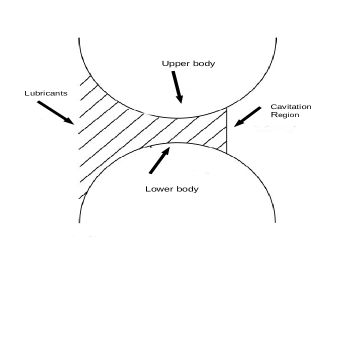
Figure 1: Undeformed surface body

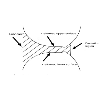
Figure 2: Deformed surface body

$$\frac{\partial}{\partial x}\Big{(}\epsilon^{*}\frac{\partial u}{\partial x}\Big{)}+\frac{\partial}{\partial y}\Big{(}\epsilon^{*}\frac{\partial u}{\partial y}\Big{)}\leq\frac{\partial(\rho h)}{\partial x}$$ (1)

$$u\geq 0$$ (2)

$$u.\Big{[}\frac{\partial}{\partial x}\Big{(}\epsilon^{*}\frac{\partial u}{\partial x}\Big{)}+\frac{\partial}{\partial y}\Big{(}\epsilon^{*}\frac{\partial u}{\partial y}\Big{)}-\frac{\partial(\rho h)}{\partial x}\Big{]}=0,$$ (3)

where $u$ is pressure of liquid and $\rho,\epsilon^{*}=\frac{\rho h_{d}^{3}}{\eta}$ are defined in appendix B. We consider above nonlinear variational inequality in a bounded, but large domain $\Omega$. Since $u$ is small on $\partial\Omega$, it seems natural to impose the boundary condition

$$u=0\quad\text{on}\quad\partial\Omega$$ (4)

The film thickness equation is in dimensionless form is written as follows

$$h_{d}(x,y)=h_{00}+\frac{x^{2}}{2}+\frac{y^{2}}{2}+\frac{2}{\pi^{2}}\int_{\Omega}\frac{u(x^{{}^{\prime}},y^{{}^{\prime}})dx^{{}^{\prime}}dy^{{}^{\prime}}}{\sqrt{(x-x^{{}^{\prime}})^{2}+(y-y^{{}^{\prime}})^{2}}}$$ (5)

where $h_{00}$ is an integration constant.
The dimensionless force balance equation is defined as follows

$$\int_{-\infty}^{\infty}\int_{-\infty}^{\infty}u(x^{\prime},y^{\prime})dx^{\prime}dy^{\prime}=\frac{3\pi}{2}$$ (6)

Consider the ball is elastic whenever load is large enough. Then system 1–6 forms an Elasto-hydrodynamic Lubrication. Schematic diagrams of EHL model is given in 1 and 2 in the form of undeformed and deformed contacting body structure respectively.
The remainder of the article is organized as follows. In section 2 variational inequality and its notation is established; Furthermore, existence results are proved for our model problem; In section. 3 DG-FVM notation and the proposed method is demonstrated; In section. 4 Error estimates are proved in $L^{2}$ and $H^{1}$ norm; In section. 5 numerical experiment and graphical results are provided; At last section. 6 conclusion and future direction is mentioned.

2 Variational Inequality

We consider space $\mathscr{V}=H^{1}_{0}(\Omega)$ and its dual space as $\mathscr{V}^{*}=(H^{1}_{0}(\Omega))^{*}=H^{-1}(\Omega)$. Also define notion $\langle.,.\rangle$ as duality pairing on $\mathscr{V}^{*}\times\mathscr{V}$. Further assume that $\mathscr{C}$ is closed convex subset of $\mathscr{V}$ defined by

$$\mathscr{C}=\Big{\{}v\in\mathscr{V}:v\geq 0\text{ a.e. }\in\Omega\Big{\}}$$ (7)

Additionally, we define the operator $\mathscr{T}$ as

$$\mathscr{T}:u\rightarrow-\Big{[}\frac{\partial}{\partial x}\Big{(}\epsilon^{*}\frac{\partial u}{\partial x}\Big{)}+\frac{\partial}{\partial y}\Big{(}\epsilon^{*}\frac{\partial u}{\partial y}\Big{)}\Big{]}+\frac{\partial(\rho h_{d})}{\partial x}$$ (8)

Then, for a given $f\in\mathscr{V}^{*}$, the problem of finding an element $u\in\mathscr{C}$ such that

$$\langle\mathscr{T}(u)-f,v-u\rangle\geq 0,\quad\forall v\in\mathscr{C}.$$ (9)

Throughout in the article we shall assume that there exists $\delta>0$ and $K_{*}>0$ such that

$$\frac{\partial\epsilon(\varsigma)}{\partial u}.\nabla u\geq K_{*}|u|^{2}\quad\forall\varsigma\in\Omega\quad\forall\varsigma\in\mathcal{Z}_{\delta}$$ (10)

Definition 2.1.

Operator $\mathscr{T}:\mathscr{C}\subset\mathscr{V}\rightarrow\mathscr{V}^{*}$ is said to be pseudo-monotone if $\mathscr{T}$ is a bounded operator and whenever $u_{k}\rightharpoonup u$ in $\mathscr{V}$ as $k\rightarrow\infty$ and

$$\lim_{k\rightarrow\infty}\sup\langle\mathscr{T}(u_{k}),u_{k}-u\rangle\leq 0.$$ (11)

it follows that for all $v\in\mathscr{C}$

$$\lim_{k\rightarrow\infty}\inf\langle\mathscr{T}(u_{k}),u-v\rangle\geq\langle\mathscr{T}(u),u-v\rangle.$$ (12)

Definition 2.2.

Operator $\mathscr{T}:\mathscr{V}\rightarrow\mathscr{V}^{*}$ is said to be hemi-continuous if and only if the function $\phi:t\longmapsto\langle\mathscr{T}(tx+(1-t)y),x-y\rangle$ is continuous on $[0,1]\quad\forall x,y\in\mathscr{V}$.

On this context the following existence theorem has been proved by Oden and Wu [9] by assuming constant density and constant viscosity of the lubricant. However, idea is easily extend-able for more realistic operating condition in which density and viscosity of the lubricant are depend on its applied pressure see Appendix. B. A straight forward modification of the analysis of [9] yields the theorem below and so we will omit the proof.

Theorem 2.1.

[9] Let $\mathscr{C}(\neq\emptyset)$ be a closed, convex subset of a reflexive Banach space $\mathscr{V}$ and let $\mathscr{T}:\mathscr{C}\subset\mathscr{V}\rightarrow\mathscr{V}^{*}$ be a pseudo-monotone, bounded, and coercive operator from $\mathscr{C}$ into the dual $\mathscr{V}^{*}$ of $\mathscr{V}$, in the sense that there exists $y\in\mathscr{C}$ such that

$$\text{lim}_{||x||\rightarrow\infty}\frac{\langle\mathscr{T}(x),x-y\rangle}{||x||}=\infty.$$ (13)

Let $f$ be given in $\mathscr{V}^{*}$ then there exists at least one $u\in\mathscr{C}$ such that

$$\langle\mathscr{T}(x)-f,y-x\rangle\geq 0\quad\forall y\in\mathscr{C}.$$ (14)

In the next section, we will give a complete formulation as well as will give theoretical justification for existence of our model problem in discrete computed setting.

3 Discrete Formulation of DG-FVM

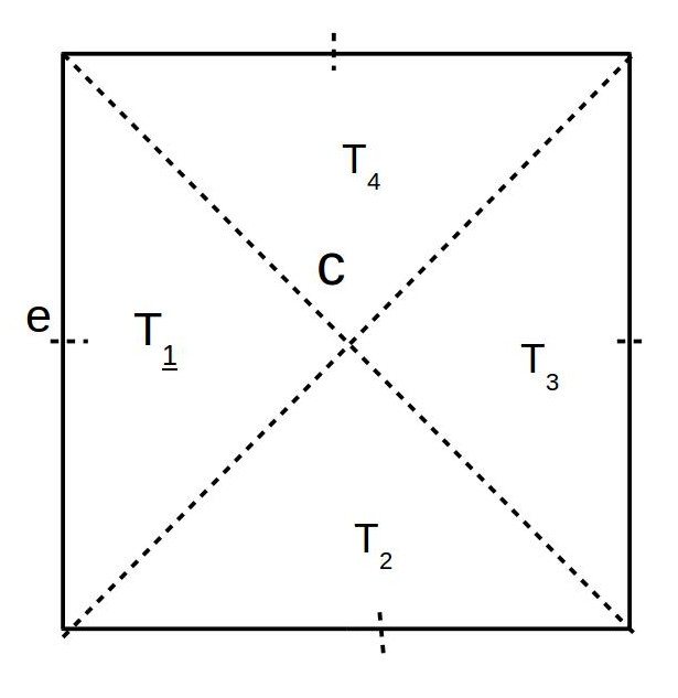
Figure 3: Rectangular partition

We define finite dimensional space associated with $\mathscr{R}_{h}$ for trial functions as

$$\mathscr{V}_{h}=\{v\in L^{2}(\Omega):v|_{K}\in\mathcal{S}_{1}(K),v|_{\partial\Omega}=0\quad\forall K\in\mathscr{R}_{h}\}.$$ (15)

Define the finite dimensional space $\mathscr{W}_{h}$ for test functions associated with the dual partition $\mathscr{M}_{h}$ as

$$\mathscr{W}_{h}=\{q\in L^{2}(\Omega):q|_{T}\in\mathcal{S}_{0}(T),q|_{\partial\Omega}=0\quad\forall T\in\mathscr{M}_{h}\},$$ (16)

where $\mathcal{S}_{l}(T)$ consist of all the polynomials with degree less than or equal to $l$ defined on $T$.
Let $\mathscr{V}(h)=\mathscr{V}_{h}+H^{2}(\Omega)\cap H^{1}_{0}(\Omega)$. Define a mapping

$$\gamma:\mathscr{V}(h)\longmapsto\mathscr{W}_{h}\quad\gamma v|_{T}=\frac{1}{h_{e}}\int_{e}v|_{T}ds,\quad T\in\mathscr{M}_{h}.$$ (17)

Let $T_{j}\in\mathscr{M}_{h}(j=1,2,3,4)$ be four triangles in $K\in\mathscr{R}_{h}$. Let $e$ be an interior edge shared by two elements $K_{1}$ and $K_{2}$ in $\mathscr{R}_{h}$ and let $\mathbb{n_{1}}$ and $\mathbb{n_{2}}$ be unit normal vectors on $e$ pointing exterior to $K_{1}$ and $K_{2}$ respectively. We define average {.} and jump [.] on $e$ for scalar $q$ and vector $w$, respectively, as ([1])

$$\{q\}=\frac{1}{2}(q|_{\partial T_{1}}+q|_{\partial T_{2}}),\quad[q]=(q|_{\partial T_{1}}\mathbb{n_{1}}+q|_{\partial T_{2}}\mathbb{n_{2}})$$

$$\{w\}=\frac{1}{2}(w|_{\partial T_{1}}+w|_{\partial T_{2}}),\quad[w]=(w|_{\partial T_{1}}\mathbb{n_{1}}+w|_{\partial T_{2}}\mathbb{n_{2}})$$

If $e$ is a edge on the boundary of $\Omega$, we define ${q}=q,\quad[w]=w.\mathbb{n}$. Let $\Gamma$ denote the union of the boundaries of the triangle $K$ of $\mathscr{R}_{h}$ and $\Gamma_{0}:=\Gamma\diagdown\partial\Omega$.

3.1 Weak Formulation

Reconsider the problem of the type

$$\frac{\partial}{\partial x}\Big{(}\epsilon^{*}\frac{\partial u}{\partial x}\Big{)}+\frac{\partial}{\partial y}\Big{(}\epsilon^{*}\frac{\partial u}{\partial y}\Big{)}-\frac{\partial(\rho h)}{\partial x}=0\quad\text{in }\Omega$$ (18)

$$u=0\quad\text{on }\partial\Omega,$$ (19)

where all notation has their usual meaning.
For given $u,v\in H^{2}(\Omega)$ and for fixed value of $\Phi\in H^{2}(\Omega)$, define bilinear form as

$$\langle\mathscr{T}(\Phi;u),v\rangle=\sum\limits_{K\in\mathscr{R}}\sum\limits_{j=1}^{4}\int_{A_{j+1}CA_{j}}\epsilon(\Phi)\nabla u.\mathbb{n}\gamma vds$$

$$+\sum\limits_{e\in\Gamma}\int_{e}[v]\{\epsilon(\Phi)\nabla u.\mathbb{n}\}ds+\alpha_{1}\sum\limits_{e\in\Gamma}[\gamma u]_{e}[v]_{e}$$

$$-\sum\limits_{K\in\mathscr{R}_{h}}\sum\limits_{j=1}^{4}\int_{A_{j+1}CA_{j}}(\rho(\Phi)h_{d}(u)).(\beta.\mathbb{n})\gamma vds-\sum\limits_{e\in\Gamma}\int_{e}[v]\{(\rho(\Phi)h_{d}(u)).(\beta.\mathbb{n})\}ds.$$ (20)

We define the following mesh dependent norm ${\left|\kern-1.07639pt\left|\kern-1.07639pt\left|.\right|\kern-1.07639pt\right|\kern-1.07639pt\right|}$ and ${\left|\kern-1.07639pt\left|\kern-1.07639pt\left|.\right|\kern-1.07639pt\right|\kern-1.07639pt\right|}_{\nu}$ as

$${\left|\kern-1.07639pt\left|\kern-1.07639pt\left|v\right|\kern-1.07639pt\right|\kern-1.07639pt\right|}^{2}=|v|^{2}_{1,h}+\sum_{e}|\gamma v|_{e}^{2}$$ (21)

$${\left|\kern-1.07639pt\left|\kern-1.07639pt\left|v\right|\kern-1.07639pt\right|\kern-1.07639pt\right|}^{2}_{\nu}=|v|^{2}_{1,h}+\sum_{e}h_{e}\int_{e}\Big{\{}\frac{\partial v}{\partial\nu}\Big{\}}^{2}ds+\sum_{e}|\gamma v|_{e}^{2},\text{ where }|v|^{2}_{1,h}=\sum_{K}|v|_{1,K}^{2}.$$ (22)

Now we will state few lemmas and inequalities without proof which will be later helpful in our subsequent analysis.

Lemma 3.1.

For $u\in H^{s}(K_{i})$, there exist a positive constant $C_{A}$ and an interpolation value $u_{I}\in\mathscr{V}_{h}$, such that

$$||u-u_{I}||_{s,K}\leq C_{A}h^{2-s}|u|_{2,K},\quad s=0,1.$$ (23)

Trace inequality. We state without proof the following trace inequality. Let $\phi\in H^{2}(K)$ and for an edge $e$ of $K$,

$$||\phi||_{e}^{2}\leq C(h_{e}^{-1}|\phi|_{K}^{2}+h_{e}|\phi|_{1,K}^{2}).$$ (24)

Lemma 3.2.

Let for any $u,v\in\mathscr{V}_{h}$, then we have following relation

$$\langle h^{3}_{d}\rho e^{-au}\nabla_{h}u,\nabla_{h}v\rangle\leq\langle\mathscr{T}_{1}(u;u_{h}),v\rangle+C_{1}h{\left|\kern-1.07639pt\left|\kern-1.07639pt\left|u\right|\kern-1.07639pt\right|\kern-1.07639pt\right|}{\left|\kern-1.07639pt\left|\kern-1.07639pt\left|v\right|\kern-1.07639pt\right|\kern-1.07639pt\right|},$$ (25)

where

$$\langle\mathscr{T}_{1}(u;u_{h}),v\rangle=\sum\limits_{K\in\mathscr{R}}\sum\limits_{j=1}^{4}\int_{A_{j+1}CA_{j}}h^{3}_{d}\rho e^{-au}\nabla u.\mathbb{n}\gamma vds$$

Proof.

Proof of lemma follows using similar argument as mentioned in [16],lemma 2.1. ∎

Next lemma provides us a bound of film thickness term and later helpful in proving coercivity and error analysis.

Lemma 3.3.

For $h_{d}$ defined in equation 5, $0<\beta_{*}<1,s=2-\beta_{*}/(1-\beta_{*})>2$ there exist $C_{1}\text{ and }C_{2}>0$ such that

$$\max_{x,y\in\Omega}|h_{d}(u)|\leq C_{1}+C_{2}\lVert u\rVert_{L^{s}}\quad 0<\beta_{*}<1,\quad\forall(x,y)\in\bar{\Omega}.$$ (26)

Lemma 3.4.

The operator $\mathscr{T}$ defined in equation LABEL:eq:34 is bounded as a map from $\mathscr{V}$ into $\mathscr{V}^{*}$.

Lemma 3.5.

The operator $\mathscr{T}$, defined in equation (21) is hemi-continuous, that is $\forall u,v,w\in\mathscr{V}$,

$$\lim_{t\rightarrow 0^{+}}\langle\mathscr{T}(u+tv),w\rangle=\langle\mathscr{T}(u),w\rangle.$$

Lemma 3.6.

The operator defined on equation (21) is coercive i.e. there is a constant $C$ independent of $h$ such that for $\alpha_{1}$ large enough and $h$ is small enough

$$\langle\mathscr{T}(u;u_{h}),u_{h}\rangle\geq C{\left|\kern-1.07639pt\left|\kern-1.07639pt\left|u_{h}\right|\kern-1.07639pt\right|\kern-1.07639pt\right|}^{2}\quad\forall u_{h}\in\mathscr{V}_{h}$$ (27)

3.2 Exterior penalty solution approximation

In this section, we introduce an exterior penalty term to regularize the inequality constraint 1–6. We define a exterior penalty operator ${\xi}:H_{0}^{1}(\Omega)\rightarrow H^{-1}$ as

$${\xi}(u)=u^{-}/\epsilon\quad\text{with }\epsilon>0,$$ (28)

where $u^{-}=u-\max(u,0)=\dfrac{u-|u|}{2}$. Let us define exterior penalty problem, $(\mathscr{U}_{\epsilon})$: for $\epsilon>0,\quad\text{find}\quad u_{\epsilon}\in\mathscr{V}_{h}$ such that

$$\langle\mathscr{T}(u_{\epsilon}^{n}),v\rangle+\langle{\xi}(u_{\epsilon}),v\rangle/\epsilon=\langle f,v\rangle\quad\forall v\in\mathscr{V}_{h},$$ (29)

Then we will show that there exist solutions $u_{\epsilon}^{n}\in\mathscr{V}_{h}$ (For proof of this we will refer to see A). This approach can be used in our DG-FVM case and modified discrete weak formulation is written as

$$\langle\mathscr{T}_{1}(u),\gamma v\rangle+\dfrac{1}{{\varepsilon}}\sum\limits_{K\in\mathscr{R}_{h}}\sum\limits_{j=1}^{4}\int_{T_{j}\subset K}u_{-}\gamma vds-\langle\mathscr{T}_{2}(u),\gamma v\rangle=0,\forall v\in\mathscr{V}_{h},$$ (30)

where ${\varepsilon}$ is an arbitrary small positive number (${\varepsilon}=1.0\times 10^{-6}$).

Lemma 3.7.

Penalty operator $\xi:\mathscr{V}\longmapsto\mathscr{V^{*}}$ is monotone, coercive and bounded.

Proof.

Now define domains $\Omega_{1}=\{x\in\Omega_{1}:u_{1}>0\}$ and $\Omega_{2}=\{x\in\Omega_{2}:u_{2}>0\}$ and their compliments as $\Omega_{1}^{c}\text{ and }\Omega_{2}^{c}$ respectively. Also consider

$$u_{i}=\begin{cases}u_{i}\in\Omega_{i}^{c}\quad\forall i=1,2\\[8.61108pt] 0\in\Omega_{i}\quad\forall i=1,2.\end{cases}$$ (31)

For proving monotonicity we consider

$$\langle\xi(u_{1})-\xi(u_{2}),u_{1}-u_{2}\rangle=\sum_{K\in\mathscr{R}_{h}}\int_{K}u_{1}^{-}(\gamma(u_{1}-u_{2}))-u_{2}^{-}(\gamma(u_{1}-u_{2}))dx$$

$$=\sum_{K\in\mathscr{R}_{h}}\int_{K}u_{1}^{-}(\gamma(u_{1}-u_{2})-(u_{1}-u_{2})+(u_{1}-u_{2}))dx$$

$$-\sum_{K\in\mathscr{R}_{h}}\int_{K}u_{2}^{-}(\gamma(u_{1}-u_{2})-(u_{1}-u_{2})+(u_{1}-u_{2}))dx$$

$$=\sum_{K\in\mathscr{R}_{h}}\int_{K\cap\Omega_{1}^{c}}u_{1}^{-}(u_{1}-u_{2})dx-\int_{K\cap\Omega_{2}^{c}}u_{2}^{-}(u_{1}-u_{2})dx$$

$$+\sum_{K\in\mathscr{R}_{h}}\int_{K\cap\Omega_{1}^{c}\cap\Omega_{2}^{c}}u_{1}^{-}(u_{1}-u_{2})-u_{2}^{-}(u_{1}-u_{2})dx$$

$$+\sum_{K\in\mathscr{R}_{h}}\int_{K\cap\Omega_{1}\cap\Omega_{2}}u_{1}^{-}(u_{1}-u_{2})-u_{2}^{-}(u_{1}-u_{2})dx$$

$$=\sum_{K\in\mathscr{R}_{h}}\int_{K\cap\Omega_{1}^{c}}u_{1}^{-}(u_{1}-u_{2})-u_{2}^{-}(u_{1}-u_{2})dx$$

$$-\sum_{K\in\mathscr{R}_{h}}\int_{K\cap\Omega_{2}^{c}}u_{1}^{-}(u_{1}-u_{2})-u_{2}^{-}(u_{1}-u_{2})dx$$

$$+\sum_{K\in\mathscr{R}_{h}}\int_{K\cap\Omega_{1}^{c}\cap\Omega_{2}^{c}}(u_{1}-u_{2})^{2}dx\geq 0$$

Hence, operator is monotone. Also, coercivity follows from the fact that

$$\langle\xi(u),u\rangle=\langle u^{-},u\rangle=\sum_{K\in\mathscr{R}_{h}}\int_{K(u\leq 0)}u^{-}\gamma udx=\sum_{K\in\mathscr{R}_{h}}\int_{K(u\leq 0)}u^{-}(\gamma u-u+u)dx$$

$$=\sum_{K\in\mathscr{R}_{h}}\int_{K(u\leq 0)}(u^{-})^{2}dx=|\lVert(u^{-})\rVert|^{2}\geq 0.$$ (32)

Furthermore, since

$$|\langle\xi(u),v\rangle|=|u^{-}\gamma v|\leq|\lVert u\rVert||\lVert v\rVert|.$$ (33)

This implies that $\xi$ is bounded. ∎

3.3 Linearization

Let us consider a fix value of $w_{u}\in H^{2}(\Omega)$ and also take $w,v\in H^{2}(\Omega)$. Furthermore, consider bilinear form $\mathscr{B}(w_{u};w,v)$ solving EHL problem defined in 1.1-1.6 as

$$\mathscr{B}(w_{u};w,v):=\sum\limits_{K\in\mathscr{R}}\sum\limits_{j=1}^{4}\int_{A_{j+1}CA_{j}}\epsilon(w_{u})\nabla w.\mathbb{n}\gamma vds$$

$$+\sum\limits_{e\in\Gamma}\int_{e}[v]\{\epsilon(w_{u})\nabla w.\mathbb{n}\}ds+\alpha_{1}\sum\limits_{e\in\Gamma}[\gamma v]_{e}[\gamma w]_{e}+\beta_{1}\langle w^{-},v\rangle$$

$$-\sum\limits_{K\in\mathscr{R}_{h}}\sum\limits_{j=1}^{4}\int_{A_{j+1}CA_{j}}(\rho(w_{u})h_{d}(x)).(\beta.\mathbb{n})\gamma vds-\sum\limits_{e\in\Gamma}\int_{e}[v]\{(\rho(w_{u})h_{d}(x)).(\beta.\mathbb{n})\}ds$$ (34)

Now define weak formulation for solving DGFVEM for solving problem 1.1-1.6 as find $u\in H^{2}(\Omega,\mathscr{R}_{h})$ such that

$$\mathscr{B}(u;u,v)=0.$$ (35)

Also $u_{h}\in\mathscr{V}_{h}\subset H^{2}(\Omega,\mathscr{R}_{h})$ so we have

$$\mathscr{B}(u;u,v)=\mathscr{B}(u_{h};u_{h},v_{h})\quad\forall v_{h}\in\mathscr{V}_{h}.$$ (36)

Since we are solving highly non-linear type of operator and so an appropriate linearizion is required for further analysis. Therefore, we use following Taylor series expansion to linearize the problem as

$$\epsilon(w)=\epsilon(u)+\tilde{\epsilon}_{u}(w)(w-u),$$ (37)

where $\tilde{\epsilon}_{u}(w)=\int_{0}^{1}\epsilon_{u}(w+\tau[w-u])d\tau$ and

$$\epsilon(w)=\epsilon(u)+{\epsilon}_{u}(w)(w-u)+\tilde{\epsilon}_{uu}(w)(w-u)^{2},$$ (38)

where $\tilde{\epsilon}_{uu}(w)=\int_{0}^{1}(1-\tau)\epsilon_{uu}(w+\tau[w-u])d\tau$. It is easy to check that $\tilde{\epsilon}_{u}\in C^{1}_{b}(\bar{\Omega},\mathcal{R})$ and $\tilde{\epsilon}_{uu}\in C^{0}_{b}(\bar{\Omega},\mathcal{R})$.
Now consider the following bilinear form $\bar{\mathscr{B}}(:,.)$ as

$$\bar{\mathscr{B}}(w_{u},w,v)=\mathscr{B}(w_{u},w,v)+\sum_{K\in\mathscr{R}_{h}}\sum_{j=1}^{4}\int_{A_{j+1}CA_{j}}(\epsilon_{u}(w_{u})\nabla w_{u})w.\gamma vds$$

$$+\sum_{e\in\Gamma}\int_{e}[\gamma v]\Big{\{}\epsilon_{u}(w_{u})\nabla w_{u}w\Big{\}}ds+\sum_{K\in\mathscr{R}_{h}}\sum_{j=1}^{4}\int_{A_{j+1}CA_{j}}\rho_{u}h_{d}w\vec{\beta}.\mathbb{n}\gamma vds$$

$$+\sum_{e\in\Gamma}\int_{e}[\gamma v]\Big{\{}\rho_{u}h_{d}w\Big{\}}ds.$$ (39)

It is easy to check that $\bar{\mathscr{B}}$ is linear in $w$ and $v$ and for fixed value of $w_{u}\in H^{2}(\Omega)$. Also as $\epsilon(w_{u})\in C^{2}_{b}(\bar{\Omega},\mathcal{R})$ and $u\in C^{2}(\bar{\Omega})$, there is a unique solution $w_{u}\in H^{2}(\Omega)$ to the following elliptic problem:

$$-\nabla.(\epsilon(u)\nabla\varphi+\epsilon_{u}\varphi\nabla u)+\nabla(\vec{\beta}(\rho h_{d}+\rho_{u}h_{d}\varphi))=\psi_{h}\text{ in }\Omega$$

$$\varphi=0\text{ on }\partial\Omega.$$ (40)

and from well known elliptic regularity property we have

$$\lVert\varphi\rVert_{H^{2}(\Omega)}\leq C\lVert\psi_{h}\rVert$$ (41)

Now for showing existence, uniqueness and for analyzing intermediate stage error analysis of discrete DGFVM solution we linearize weak formulation (35) around $\Pi_{h}u$. Let $e=u-u_{h}$ be an error term for exact and approximated DGFVM solution. Now by subtracting $\mathscr{B}(u;u_{h},u_{h})$ from both side of equation (36), we get

$$\mathscr{B}(u;e,u_{h})=\sum_{K\in\mathscr{R}_{h}}\sum_{j=1}^{4}\int_{A_{j+1}CA_{j}}(\epsilon(u_{h})-\epsilon(u))\nabla u_{h}.\mathbb{n}\gamma v_{h}ds$$

$$+\sum_{e\in\Gamma}\int_{e}[\gamma v_{h}](\epsilon(u_{h})-\epsilon(u))\nabla u_{h}ds$$

$$-\sum_{K\in\mathscr{R}_{h}}\sum_{j=1}^{4}\int_{A_{j+1}CA_{j}}(\rho(u_{h}h_{d}(x))-\rho(u)h_{d}(x))\vec{\beta}.\mathbb{n}\gamma v_{h}ds$$

$$-\sum_{e\in\Gamma}\int_{e}[\gamma v_{h}]\Big{\{}\rho(u_{h}h_{d}(x))-\rho(u)h_{d}(x)\vec{\beta}.\mathbb{n}\Big{\}}ds$$ (42)

Now adding both side in above equation following term

$$\sum_{K\in\mathscr{R}_{h}}\sum_{j=1}^{4}\int_{A_{j+1}CA_{j}}\epsilon_{u}(u_{h})(u_{h}-u)\nabla u.\mathbb{n}\gamma v_{h}ds+\sum_{e\in\Gamma}\int_{e}[\gamma v_{h}]\Big{\{}\epsilon_{u}(u_{h})(u_{h}-u)\nabla u\Big{\}}ds$$

$$-\sum_{K\in\mathscr{R}_{h}}\sum_{j=1}^{4}\int_{A_{j+1}CA_{j}}(\rho h_{d})_{u}(u_{h})(u_{h}-u)\vec{\beta}.\mathbb{n}\gamma v_{h}ds-\sum_{e\in\Gamma}\int_{e}[\gamma v_{h}]\{(\rho h_{d})_{u}(u_{h})(u_{h}-u)\}ds.$$ (43)

Now we split error term as

$$e=u-u_{h}=u-{\Pi}_{h}u+{\Pi}_{h}u-u_{h}$$

and using Taylor’s formula for linearizion given in ()-() we rewrite equation (42) as

$$\bar{\mathscr{B}}(u;{\Pi}_{h}u-u_{h},v_{h})=\bar{\mathscr{B}}(u;{\Pi}_{h}u-u,v_{h})+\mathscr{F}(u_{h};u_{h}-u,v_{h}),$$ (44)

where

$$\mathscr{F}(u_{h};u_{h}-u,v_{h})=\sum_{K\in\mathscr{R}_{h}}\sum_{j=1}^{4}\int_{A_{j+1}CA_{j}}\tilde{\epsilon}_{u}(u_{h})e\nabla e.\mathbb{n}\gamma v_{h}ds$$

$$+\sum_{e\in\Gamma}\int_{e}[\gamma v_{h}]\Big{\{}\epsilon_{u}(u_{h})e\nabla e\Big{\}}ds+\sum_{K\in\mathscr{R}_{h}}\sum_{j=1}^{4}\int_{A_{j+1}CA_{j}}\tilde{\epsilon}_{uu}(u_{h})e^{2}\nabla u.\mathbb{n}\gamma v_{h}ds$$

$$-\sum_{K\in\mathscr{R}_{h}}\sum_{j=1}^{4}\int_{A_{j+1}CA_{j}}\tilde{(\rho h_{d})}_{uu}(u_{h})e^{2}\vec{\beta}.\mathbb{n}\gamma v_{h}ds-\sum_{e\in\Gamma}\int_{e}[\gamma v_{h}]\Big{\{}(\rho h_{d})_{uu}(u_{h})e^{2}\Big{\}}ds$$ (45)

Note that solving (35) is equivalent to solving (45). Now for showing there exist at least one $u_{h}\in\mathscr{V}_{h}$ solution to the above equation (45) we consider a map

$$\mathcal{S}:\mathscr{V}_{h}\rightarrow\mathscr{V}_{h}$$

defined as $\mathcal{S}(u_{\varphi})=\varphi\in\mathscr{V}_{h},\quad\forall u_{\varphi}\in\mathscr{V}_{h}$ such that

$$\bar{\mathscr{B}}(u;{\Pi}_{h}u-\varphi,v_{h})=\bar{\mathscr{B}}(u;{\Pi}_{h}u-u,v_{h})+\mathscr{F}(u_{\varphi};u_{\varphi}-u,v_{h})$$ (46)

holds. Consider the closed neighborhood $\mathcal{Q}_{\delta}(\Pi_{h}u)$ of the diameter $\delta>0$.

$$\mathcal{Q}_{\delta}(\Pi_{h}u)=\Big{\{}u_{\varphi}\in\mathscr{V}_{h}:{\left|\kern-1.07639pt\left|\kern-1.07639pt\left|u_{\varphi}-\Pi_{h}u\right|\kern-1.07639pt\right|\kern-1.07639pt\right|}\leq\delta\Big{\}}.$$

Now we first show that $\mathcal{S}$ map closed neighborhood $\mathcal{Q}_{\delta}(\Pi_{h}u)$ into itself and then prove existence of DGFVM solution by exploiting Browder’s fixed point theorem. The proof can be break using following lemmas.

Lemma 3.8.

Let $u_{\varphi},v_{h}\in\mathscr{V}_{h}$ also set $\chi=u_{\varphi}-\Pi_{h}u$ and $\eta=u-\Pi_{h}u$. Then there exists a constant $C\geq 0$ (independent of $h$) such that

$$|\mathscr{F}(u_{\varphi};u_{\varphi}-u,v_{h})|\leq C_{\epsilon}\Big{[}{\left|\kern-1.07639pt\left|\kern-1.07639pt\left|\chi\right|\kern-1.07639pt\right|\kern-1.07639pt\right|}^{2}+C_{u}(h^{5/3}+h^{1/2}+h+h^{2/3}+h^{3/2}){\left|\kern-1.07639pt\left|\kern-1.07639pt\left|\chi\right|\kern-1.07639pt\right|\kern-1.07639pt\right|}$$

$$+C_{u}(h^{2}+h+h^{3/2}){\left|\kern-1.07639pt\left|\kern-1.07639pt\left|\eta\right|\kern-1.07639pt\right|\kern-1.07639pt\right|}\Big{]}{\left|\kern-1.07639pt\left|\kern-1.07639pt\left|v_{h}\right|\kern-1.07639pt\right|\kern-1.07639pt\right|}+C_{\rho h_{d}}\Big{[}{\left|\kern-1.07639pt\left|\kern-1.07639pt\left|\chi\right|\kern-1.07639pt\right|\kern-1.07639pt\right|}^{2}+C_{u}(h^{5/3}+h^{3/2}){\left|\kern-1.07639pt\left|\kern-1.07639pt\left|\chi\right|\kern-1.07639pt\right|\kern-1.07639pt\right|}$$

$$+C_{u}(h^{3/2}+h){\left|\kern-1.07639pt\left|\kern-1.07639pt\left|\eta\right|\kern-1.07639pt\right|\kern-1.07639pt\right|}\Big{]}{\left|\kern-1.07639pt\left|\kern-1.07639pt\left|v_{h}\right|\kern-1.07639pt\right|\kern-1.07639pt\right|}.$$ (47)

Proof.

Let $u_{\varphi}\in\mathscr{V}_{h}$ and take $\zeta=u_{\varphi}-u$ in equation (45) we write $u_{\varphi}$ in place of $u_{h}$ and $\zeta=u_{\varphi}-u$ to get

$$\mathscr{F}(u_{\varphi};\zeta,v_{h})=\sum_{K\in\mathscr{R}_{h}}\sum_{j=1}^{4}\int_{A_{j+1}CA_{j}}\tilde{\epsilon}_{u}(u_{\varphi})\zeta\nabla\zeta.\mathbb{n}\gamma v_{h}ds$$

$$+\sum_{e\in\Gamma}\int_{e}[\gamma v_{h}]\Big{\{}\epsilon_{u}(u_{\varphi})\zeta\nabla\zeta\Big{\}}ds+\sum_{K\in\mathscr{R}_{h}}\sum_{j=1}^{4}\int_{A_{j+1}CA_{j}}\tilde{\epsilon}_{uu}(u_{\varphi})\zeta^{2}\nabla u.\mathbb{n}\gamma v_{h}ds$$

$$-\sum_{K\in\mathscr{R}_{h}}\sum_{j=1}^{4}\int_{A_{j+1}CA_{j}}\tilde{(\rho h_{d})}_{uu}(u_{\varphi})\zeta^{2}\vec{\beta}.\mathbb{n}\gamma v_{h}ds-\sum_{e\in\Gamma}\int_{e}[\gamma v_{h}]\Big{\{}(\rho h_{d})_{uu}(u_{\varphi})\zeta^{2}\Big{\}}ds.$$ (48)

Now split $\zeta=\chi-\eta$ where $\chi=u_{\varphi}-\Pi_{h}u$ and $\eta=u-\Pi_{h}u$. Then right hand side is estimated in following way. The First term is estimated as

$$\Big{|}\sum_{K\in\mathscr{R}_{h}}\sum_{j=1}^{4}\int_{A_{j+1}CA_{j}}\tilde{\epsilon}_{u}(u_{\varphi})\zeta\nabla\zeta.\mathbb{n}\gamma v_{h}ds\Big{|}\leq\Big{|}\sum_{K\in\mathscr{R}_{h}}\sum_{j=1}^{4}\int_{A_{j+1}CA_{j}}\tilde{\epsilon}_{u}(u_{\varphi})\chi\nabla\chi.\mathbb{n}\gamma v_{h}ds\Big{|}$$

$$+\Big{|}\sum_{K\in\mathscr{R}_{h}}\sum_{j=1}^{4}\int_{A_{j+1}CA_{j}}\tilde{\epsilon}_{u}(u_{\varphi})\chi\nabla\eta.\mathbb{n}\gamma v_{h}ds\Big{|}+\Big{|}\sum_{K\in\mathscr{R}_{h}}\sum_{j=1}^{4}\int_{A_{j+1}CA_{j}}\tilde{\epsilon}_{u}(u_{\varphi})\eta\nabla\chi.\mathbb{n}\gamma v_{h}ds\Big{|}$$

$$+\Big{|}\sum_{K\in\mathscr{R}_{h}}\sum_{j=1}^{4}\int_{A_{j+1}CA_{j}}\tilde{\epsilon}_{u}(u_{\varphi})\eta\nabla\eta.\mathbb{n}\gamma v_{h}ds\Big{|}.$$ (49)

Second term is estimated as

$$\Big{|}\sum_{e\in\Gamma}\int_{e}[\gamma v_{h}]\Big{\{}\epsilon_{u}(u_{\varphi})\zeta\nabla\zeta\Big{\}}ds\Big{|}\leq\Big{|}\sum_{e\in\Gamma}\int_{e}[\gamma v_{h}]\Big{\{}\epsilon_{u}(u_{\varphi})\chi\nabla\chi\Big{\}}ds\Big{|}$$

$$+\Big{|}\sum_{e\in\Gamma}\int_{e}[\gamma v_{h}]\Big{\{}\epsilon_{u}(u_{\varphi})\eta\nabla\chi\Big{\}}ds\Big{|}+\Big{|}\sum_{e\in\Gamma}\int_{e}[\gamma v_{h}]\Big{\{}\epsilon_{u}(u_{\varphi})\chi\nabla\eta\Big{\}}ds\Big{|}$$

$$+\Big{|}\sum_{e\in\Gamma}\int_{e}[\gamma v_{h}]\Big{\{}\epsilon_{u}(u_{\varphi})\eta\nabla\eta\Big{\}}ds\Big{|}.$$ (50)

Third term is estimated as

$$\Big{|}\sum_{K\in\mathscr{R}_{h}}\sum_{j=1}^{4}\int_{A_{j+1}CA_{j}}\tilde{\epsilon}_{uu}(u_{\varphi})\zeta^{2}\nabla u.\mathbb{n}\gamma v_{h}ds\Big{|}\leq\Big{|}\sum_{K\in\mathscr{R}_{h}}\sum_{j=1}^{4}\int_{A_{j+1}CA_{j}}\tilde{\epsilon}_{uu}(u_{\varphi})\eta^{2}\nabla u.\mathbb{n}\gamma v_{h}ds\Big{|}$$

$$+2\Big{|}\sum_{K\in\mathscr{R}_{h}}\sum_{j=1}^{4}\int_{A_{j+1}CA_{j}}\tilde{\epsilon}_{uu}(u_{\varphi})\eta.\chi\nabla u.\mathbb{n}\gamma v_{h}ds\Big{|}+\Big{|}\sum_{K\in\mathscr{R}_{h}}\sum_{j=1}^{4}\int_{A_{j+1}CA_{j}}\tilde{\epsilon}_{uu}(u_{\varphi})\chi^{2}\nabla u.\mathbb{n}\gamma v_{h}ds\Big{|}.$$ (51)

Fourth term is estimated as

$$\Big{|}\sum_{K\in\mathscr{R}_{h}}\sum_{j=1}^{4}\int_{A_{j+1}CA_{j}}\tilde{(\rho h_{d})}_{uu}(u_{\varphi})\zeta^{2}\vec{\beta}.\mathbb{n}\gamma v_{h}ds\Big{|}\leq\Big{|}\sum_{K\in\mathscr{R}_{h}}\sum_{j=1}^{4}\int_{A_{j+1}CA_{j}}\tilde{(\rho h_{d})}_{uu}(u_{\varphi})\chi^{2}\vec{\beta}.\mathbb{n}\gamma v_{h}ds\Big{|}$$

$$+2\Big{|}\sum_{K\in\mathscr{R}_{h}}\sum_{j=1}^{4}\int_{A_{j+1}CA_{j}}\tilde{(\rho h_{d})}_{uu}(u_{\varphi})\eta.\chi\vec{\beta}.\mathbb{n}\gamma v_{h}ds\Big{|}+\Big{|}\sum_{K\in\mathscr{R}_{h}}\sum_{j=1}^{4}\int_{A_{j+1}CA_{j}}\tilde{(\rho h_{d})}_{uu}(u_{\varphi})\eta^{2}\vec{\beta}.\mathbb{n}\gamma v_{h}ds\Big{|}.$$ (52)

Fifth term is estimated as

$$\Big{|}\sum_{e\in\Gamma}\int_{e}[\gamma v_{h}]\Big{\{}(\rho h_{d})_{uu}(u_{\varphi})\zeta^{2}\Big{\}}ds\Big{|}\leq\Big{|}\sum_{e\in\Gamma}\int_{e}[\gamma v_{h}]\Big{\{}(\rho h_{d})_{uu}(u_{\varphi})\chi^{2}\Big{\}}ds\Big{|}$$

$$+2\Big{|}\sum_{e\in\Gamma}\int_{e}[\gamma v_{h}]\Big{\{}(\rho h_{d})_{uu}(u_{\varphi})\eta.\chi\Big{\}}ds\Big{|}+\Big{|}\sum_{e\in\Gamma}\int_{e}[\gamma v_{h}]\Big{\{}(\rho h_{d})_{uu}(u_{\varphi})\eta^{2}\Big{\}}ds\Big{|}.$$ (53)

In equation (49) first term is estimated as

$$\Big{|}\sum_{K\in\mathscr{R}_{h}}\sum_{j=1}^{4}\int_{A_{j+1}CA_{j}}\tilde{\epsilon}_{u}(u_{\varphi})\chi\nabla\chi.\mathbb{n}\gamma v_{h}ds\Big{|}\leq\Big{|}\sum_{K}\langle{\epsilon}_{u}(u_{\varphi})\chi\nabla\chi,\nabla v_{h}\rangle\Big{|}$$

$$+\Big{|}\sum_{K}\int_{\partial K}[\gamma v_{h}-v_{h}]\Big{\{}{\epsilon}_{u}(u_{\varphi})\chi\nabla\chi.\mathbb{n}\Big{\}}ds\Big{|}+\Big{|}\sum_{K}\langle\nabla\Big{(}{\epsilon}_{u}(u_{\varphi})\chi\nabla\chi\Big{)},v_{h}-\gamma v_{h}\rangle\Big{|}.$$ (54)

First part of equation (54) is estimated as

$$\Big{|}\sum_{K}\langle{\epsilon}_{u}(u_{\varphi})\chi\nabla\chi,\nabla v_{h}\rangle\Big{|}\leq C_{\epsilon}\sum_{K}\int_{K}|\chi.\nabla\chi.\nabla v_{h}|dx.$$

Now using holder’s inequality we get

$$C_{\epsilon}\sum_{K}\int_{K}|\chi.\nabla\chi.\nabla v_{h}|dx\leq C_{\epsilon}\sum_{K}\lVert\chi\rVert_{L^{6}(K)}\lVert\chi\rVert_{L^{3}(K)}\lVert\nabla v_{h}\rVert_{L^{2}(K)}$$

$$\leq C_{\epsilon}{\left|\kern-1.07639pt\left|\kern-1.07639pt\left|\chi\right|\kern-1.07639pt\right|\kern-1.07639pt\right|}{\left|\kern-1.07639pt\left|\kern-1.07639pt\left|\chi\right|\kern-1.07639pt\right|\kern-1.07639pt\right|}{\left|\kern-1.07639pt\left|\kern-1.07639pt\left|v_{h}\right|\kern-1.07639pt\right|\kern-1.07639pt\right|}.$$ (55)

Now second part of equation (54) is estimated using Holder’s inequality and trace inequality

$$\Big{|}\sum_{K}\int_{\partial K}[\gamma v_{h}-v_{h}]\Big{\{}{\epsilon}_{u}(u_{\varphi})\chi\nabla\chi.\mathbb{n}\Big{\}}ds\Big{|}\leq$$

$$C_{\epsilon}\sum_{K}\Big{(}\int_{\partial K}[\gamma v_{h}-v_{h}]^{2}\Big{)}^{1/2}\lVert\chi\rVert_{L^{4}(\partial K)}\lVert\nabla\chi\rVert_{L^{4}(\partial K)}.$$

Now using trace inequality defined as

$$\lVert\nabla\chi\rVert_{L^{4}(\partial K)}\leq C_{h}\Big{(}h^{-1}\lVert\nabla\chi\rVert^{4}_{L^{4}(K)}+\lVert\nabla\chi\rVert^{3}_{L^{6}(K)}\lVert\nabla.\nabla\chi\rVert_{L^{2}(K)}\Big{)}$$ (56)

$$\lVert\chi\rVert_{L^{4}(\partial K)}\leq C_{h}\Big{(}h^{-1}\lVert\chi\rVert^{4}_{L^{4}(K)}+\lVert\chi\rVert^{3}_{L^{6}(K)}\lVert\chi\rVert_{L^{2}(K)}\Big{)}$$ (57)

we get that

$$\leq C_{\epsilon}\Big{(}h^{-1}|\gamma v_{h}-v_{h}|^{2}_{L^{2}(K)}+h|\gamma v_{h}-v_{h}|^{2}_{H^{1}(K)}\Big{)}^{1/2}\times$$

$$\Big{(}h^{-1}\lVert\chi\rVert^{4}_{L^{4}(K)}+\lVert\chi\rVert^{3}_{L^{6}(K)}\lVert\chi\rVert_{L^{2}(K)}\Big{)}^{1/4}$$

$$\times\Big{(}h^{-1}\lVert\nabla\chi\rVert^{4}_{L^{4}(K)}+\lVert\nabla\chi\rVert^{3}_{L^{6}(K)}\lVert\nabla.\nabla\chi\rVert_{L^{2}(K)}\Big{)}^{1/4}$$

$$\leq C_{\epsilon}{\left|\kern-1.07639pt\left|\kern-1.07639pt\left|\chi\right|\kern-1.07639pt\right|\kern-1.07639pt\right|}{\left|\kern-1.07639pt\left|\kern-1.07639pt\left|\chi\right|\kern-1.07639pt\right|\kern-1.07639pt\right|}{\left|\kern-1.07639pt\left|\kern-1.07639pt\left|v_{h}\right|\kern-1.07639pt\right|\kern-1.07639pt\right|}$$ (58)

Third term of equation (54) is estimated in similar way and it is written as

$$\Big{|}\sum_{K}\langle\nabla\Big{(}{\epsilon}_{u}(u_{\varphi})\chi\nabla\chi\Big{)},v_{h}-\gamma v_{h}\rangle\Big{|}\leq C_{\epsilon}{\left|\kern-1.07639pt\left|\kern-1.07639pt\left|\chi\right|\kern-1.07639pt\right|\kern-1.07639pt\right|}{\left|\kern-1.07639pt\left|\kern-1.07639pt\left|\chi\right|\kern-1.07639pt\right|\kern-1.07639pt\right|}{\left|\kern-1.07639pt\left|\kern-1.07639pt\left|v_{h}\right|\kern-1.07639pt\right|\kern-1.07639pt\right|}.$$ (59)

Now second term equation (49) is estimated as

$$\Big{|}\sum_{K\in\mathscr{R}_{h}}\sum_{j=1}^{4}\int_{A_{j+1}CA_{j}}\tilde{\epsilon}_{u}(u_{\varphi})\chi\nabla\eta.\mathbb{n}\gamma v_{h}ds\Big{|}\leq\Big{|}\sum_{K}\langle{\epsilon}_{u}(u_{\varphi})\chi\nabla\eta,\nabla v_{h}\rangle\Big{|}$$

$$+\Big{|}\sum_{K}\int_{\partial K}[\gamma v_{h}-v_{h}]\Big{\{}{\epsilon}_{u}(u_{\varphi})\chi\nabla\eta.\mathbb{n}\Big{\}}ds\Big{|}+\Big{|}\sum_{K}\langle\nabla\Big{(}{\epsilon}_{u}(u_{\varphi})\chi\nabla\eta\Big{)},v_{h}-\gamma v_{h}\rangle\Big{|}.$$ (60)

Now first term of equation (60) is estimated using Holder’s inequality as

$$\Big{|}\sum_{K}\langle{\epsilon}_{u}(u_{\varphi})\chi\nabla\eta,\nabla v_{h}\rangle\Big{|}\leq C_{\epsilon}\sum_{K}\int_{K}|\chi.\nabla\eta.\nabla v_{h}|dx$$

$$\leq C_{\epsilon}\sum_{K}\|\chi\|_{L^{6}(K)}\|\nabla\eta\|_{L^{3}(K)}\|\nabla v_{h}\|_{L^{2}(K)}$$ (61)

Now using inverse inequality defined as

$$\|v_{h}\|_{L^{r}(K)}\leq Ch^{2/r-1}\|v_{h}\|_{L^{2}(K)}\quad\forall r\geq 2.$$ (62)

and also using approximation property we get

$$\leq C_{\epsilon}C_{u}h^{-1/3}\|\nabla\eta\|_{L^{2}(K)}{\left|\kern-1.07639pt\left|\kern-1.07639pt\left|\chi\right|\kern-1.07639pt\right|\kern-1.07639pt\right|}{\left|\kern-1.07639pt\left|\kern-1.07639pt\left|v_{h}\right|\kern-1.07639pt\right|\kern-1.07639pt\right|}$$

$$\leq C_{\epsilon}C_{u}h^{2/3}\|u\|_{H^{2}(\Omega)}{\left|\kern-1.07639pt\left|\kern-1.07639pt\left|\chi\right|\kern-1.07639pt\right|\kern-1.07639pt\right|}{\left|\kern-1.07639pt\left|\kern-1.07639pt\left|v_{h}\right|\kern-1.07639pt\right|\kern-1.07639pt\right|}.$$ (63)

Second term of equation (60) is estimated as using Holder’s inequality and trace inequality

$$\Big{|}\sum_{K}\int_{\partial K}[\gamma v_{h}-v_{h}]\Big{\{}{\epsilon}_{u}(u_{\varphi})\chi\nabla\eta.\mathbb{n}\Big{\}}ds\Big{|}\leq C_{\epsilon}\sum_{K}\Big{(}\int_{\partial K}[\gamma v_{h}-v_{h}]^{2}\Big{)}^{1/2}\|\chi\|_{L^{4}(\partial K)}\|\nabla\eta\|_{L^{4}(\partial K)}$$

$$\leq C_{\epsilon}h^{-1}\sum_{K}\Big{(}|\gamma v_{h}-v_{h}|^{2}_{L^{2}(K)}+h^{2}|\gamma v_{h}-v_{h}|^{2}_{H^{1}(K)}\Big{)}^{1/2}\times\Big{(}\|\chi\|^{4}_{L^{4}(K)}+h\|\chi\|^{3}_{L^{6}(K)}\|\nabla\chi\|_{L^{2}(K)}\Big{)}^{1/4}$$

$$\times\Big{(}\|\nabla\eta\|^{4}_{L^{4}(K)}+h\|\nabla\eta\|^{3}_{L^{6}(K)}\|\nabla.\nabla\eta\|_{L^{2}(K)}\Big{)}^{1/4}$$

$$\leq C_{\epsilon}h^{1/2}\|u\|_{H^{2}(\Omega)}{\left|\kern-1.07639pt\left|\kern-1.07639pt\left|v_{h}\right|\kern-1.07639pt\right|\kern-1.07639pt\right|}{\left|\kern-1.07639pt\left|\kern-1.07639pt\left|\chi\right|\kern-1.07639pt\right|\kern-1.07639pt\right|}.$$ (64)

Third term of equation (60) is estimated as

$$\Big{|}\sum_{K}\langle\nabla\Big{(}{\epsilon}_{u}(u_{\varphi})\chi\nabla\eta\Big{)},v_{h}-\gamma v_{h}\rangle\Big{|}\leq C_{\epsilon}C_{u}(h^{2/3}\|u\|_{H^{2}(K)}{\left|\kern-1.07639pt\left|\kern-1.07639pt\left|\chi\right|\kern-1.07639pt\right|\kern-1.07639pt\right|}{\left|\kern-1.07639pt\left|\kern-1.07639pt\left|v_{h}\right|\kern-1.07639pt\right|\kern-1.07639pt\right|}$$

$$+h^{1/2}\|u\|_{H^{2}(\Omega)}{\left|\kern-1.07639pt\left|\kern-1.07639pt\left|v_{h}\right|\kern-1.07639pt\right|\kern-1.07639pt\right|}{\left|\kern-1.07639pt\left|\kern-1.07639pt\left|\chi\right|\kern-1.07639pt\right|\kern-1.07639pt\right|}).$$ (65)

Now third term of equation (49) is estimated as

$$\Big{|}\sum_{K\in\mathscr{R}_{h}}\sum_{j=1}^{4}\int_{A_{j+1}CA_{j}}\tilde{\epsilon}_{u}(u_{\varphi})\eta\nabla\chi.\mathbb{n}\gamma v_{h}ds\Big{|}\leq\Big{|}\sum_{K}\langle{\epsilon}_{u}(u_{\varphi})\eta\nabla\chi,\nabla v_{h}\rangle\Big{|}$$

$$+\Big{|}\sum_{K}\int_{\partial K}[\gamma v_{h}-v_{h}]\Big{\{}{\epsilon}_{u}(u_{\varphi})\eta\nabla\chi.\mathbb{n}\Big{\}}ds\Big{|}+\Big{|}\sum_{K}\langle\nabla\Big{(}{\epsilon}_{u}(u_{\varphi})\eta\nabla\chi\Big{)},v_{h}-\gamma v_{h}\rangle\Big{|}.$$ (66)

First part of equation (66) is estimated by using Holder’s inequality as

$$\Big{|}\sum_{K}\langle{\epsilon}_{u}(u_{\varphi})\eta\nabla\chi,\nabla v_{h}\rangle\Big{|}\leq C_{\epsilon}\sum_{K}\|\eta\|_{L^{6}(K)}\|\nabla\chi\|_{L^{3}(K)}\|\nabla v_{h}\|_{L^{2}(K)}$$

$$\leq C_{\epsilon}\sum_{K}h^{2/6-1}\|\eta\|_{L^{2}(K)}h^{2/3-1}\|\nabla\chi\|_{L^{2}(K)}\|\nabla v_{h}\|_{L^{2}(K)}$$

$$\leq C_{\epsilon}C_{u}h\|u\|_{H^{2}(\Omega)}{\left|\kern-1.07639pt\left|\kern-1.07639pt\left|\chi\right|\kern-1.07639pt\right|\kern-1.07639pt\right|}{\left|\kern-1.07639pt\left|\kern-1.07639pt\left|v_{h}\right|\kern-1.07639pt\right|\kern-1.07639pt\right|}.$$ (67)

Second part of equation (66) is estimated using trace inequality we have

$$\Big{|}\sum_{K}\int_{\partial K}[\gamma v_{h}-v_{h}]\Big{\{}{\epsilon}_{u}(u_{\varphi})\eta\nabla\chi.\mathbb{n}\Big{\}}ds\Big{|}\leq C_{\epsilon}\sum_{K}\Big{(}\int_{\partial K}[\gamma v_{h}-v_{h}]^{2}ds\Big{)}^{1/2}\|\eta\|_{L^{4}(\partial K)}\|\nabla\chi\|_{L^{4}(\partial K)}$$

$$\leq C_{\epsilon}h^{3/2}\|u\|_{H^{2}(\Omega)}{\left|\kern-1.07639pt\left|\kern-1.07639pt\left|\chi\right|\kern-1.07639pt\right|\kern-1.07639pt\right|}{\left|\kern-1.07639pt\left|\kern-1.07639pt\left|v_{h}\right|\kern-1.07639pt\right|\kern-1.07639pt\right|}$$ (68)

Third part of equation (66) is estimated as

$$\Big{|}\sum_{K}\langle\nabla\Big{(}{\epsilon}_{u}(u_{\varphi})\eta\nabla\chi\Big{)},v_{h}-\gamma v_{h}\rangle\Big{|}\leq C_{\epsilon}C_{u}h\|u\|_{H^{2}(\Omega)}{\left|\kern-1.07639pt\left|\kern-1.07639pt\left|\chi\right|\kern-1.07639pt\right|\kern-1.07639pt\right|}{\left|\kern-1.07639pt\left|\kern-1.07639pt\left|v_{h}\right|\kern-1.07639pt\right|\kern-1.07639pt\right|}+C_{\epsilon}h^{3/2}\|u\|_{H^{2}(\Omega)}{\left|\kern-1.07639pt\left|\kern-1.07639pt\left|\chi\right|\kern-1.07639pt\right|\kern-1.07639pt\right|}{\left|\kern-1.07639pt\left|\kern-1.07639pt\left|v_{h}\right|\kern-1.07639pt\right|\kern-1.07639pt\right|}$$ (69)

Fourth term of equation (49) is estimated as

$$\Big{|}\sum_{K\in\mathscr{R}_{h}}\sum_{j=1}^{4}\int_{A_{j+1}CA_{j}}\tilde{\epsilon}_{u}(u_{\varphi})\eta\nabla\eta.\mathbb{n}\gamma v_{h}ds\Big{|}\leq\Big{|}\sum_{K}\langle{\epsilon}_{u}(u_{\varphi})\eta\nabla\eta,\nabla v_{h}\rangle\Big{|}$$

$$+\Big{|}\sum_{K}\int_{\partial K}[\gamma v_{h}-v_{h}]\Big{\{}{\epsilon}_{u}(u_{\varphi})\eta\nabla\eta.\mathbb{n}\Big{\}}ds\Big{|}+\Big{|}\sum_{K}\langle\nabla\Big{(}{\epsilon}_{u}(u_{\varphi})\eta\nabla\eta\Big{)},v_{h}-\gamma v_{h}\rangle\Big{|}.$$ (70)

First part of equation (70) is estimated using Holder’s inequality as

$$\Big{|}\sum_{K}\langle{\epsilon}_{u}(u_{\varphi})\eta\nabla\eta,\nabla v_{h}\rangle\Big{|}\leq C_{\epsilon}\sum_{K}\|\eta\|_{L^{6}(K)}\|\nabla\eta\|_{L^{3}(K)}\|\nabla v_{h}\|_{L^{2}(K)}$$

$$\leq C_{\epsilon}C_{u}h\|u\|_{H^{2}(\Omega)}{\left|\kern-1.07639pt\left|\kern-1.07639pt\left|\eta\right|\kern-1.07639pt\right|\kern-1.07639pt\right|}{\left|\kern-1.07639pt\left|\kern-1.07639pt\left|v_{h}\right|\kern-1.07639pt\right|\kern-1.07639pt\right|}$$ (71)

Second part of equation (70) is estimated as

$$\Big{|}\sum_{K}\int_{\partial K}[\gamma v_{h}-v_{h}]\Big{\{}{\epsilon}_{u}(u_{\varphi})\eta\nabla\eta.\mathbb{n}\Big{\}}ds\Big{|}\leq C_{\epsilon}\sum_{K}\Big{(}\int_{\partial K}[\gamma v_{h}-v_{h}]^{2}ds\Big{)}^{1/2}\|\eta\|_{L^{4}(\partial K)}\|\nabla\eta\|_{L^{4}(\partial K)}$$

$$\leq C_{\epsilon}h^{3/2}\|u\|_{H^{2}(\Omega)}{\left|\kern-1.07639pt\left|\kern-1.07639pt\left|\eta\right|\kern-1.07639pt\right|\kern-1.07639pt\right|}{\left|\kern-1.07639pt\left|\kern-1.07639pt\left|v_{h}\right|\kern-1.07639pt\right|\kern-1.07639pt\right|}$$ (72)

Third part of equation (70) is estimated as

$$\Big{|}\sum_{K}\langle\nabla\Big{(}{\epsilon}_{u}(u_{\varphi})\eta\nabla\eta\Big{)},v_{h}-\gamma v_{h}\rangle\Big{|}\leq C_{\epsilon}C_{u}h\|u\|_{H^{2}(\Omega)}{\left|\kern-1.07639pt\left|\kern-1.07639pt\left|\eta\right|\kern-1.07639pt\right|\kern-1.07639pt\right|}{\left|\kern-1.07639pt\left|\kern-1.07639pt\left|v_{h}\right|\kern-1.07639pt\right|\kern-1.07639pt\right|}+C_{\epsilon}h^{3/2}\|u\|_{H^{2}(\Omega)}{\left|\kern-1.07639pt\left|\kern-1.07639pt\left|\eta\right|\kern-1.07639pt\right|\kern-1.07639pt\right|}{\left|\kern-1.07639pt\left|\kern-1.07639pt\left|v_{h}\right|\kern-1.07639pt\right|\kern-1.07639pt\right|}.$$ (73)

Now first part of equation (50) is estimated as

$$\Big{|}\sum_{e\in\Gamma}\int_{e}[\gamma v_{h}]\Big{\{}\epsilon_{u}(u_{\varphi})\chi\nabla\chi\Big{\}}ds\Big{|}\leq C_{\epsilon}\sum_{K}\Big{(}[\gamma v_{h}]^{2}\Big{)}^{1/2}\|\chi\|_{L^{4}(\partial K)}\|\nabla\chi\|_{L^{4}(\partial K)}$$

$$\leq C_{\epsilon}\sum_{K}\Big{(}[\gamma v_{h}]^{2}\Big{)}^{1/2}\Big{(}\|\chi\|^{4}_{L^{4}(K)}+h\|\chi\|^{3}_{L^{6}(K)}\|\nabla\chi\|_{L^{2}(K)}\Big{)}^{1/4}$$

$$\times\Big{(}\|\nabla\chi\|^{4}_{L^{4}(K)}+h\|\nabla\chi\|^{3}_{L^{6}(K)}\|\nabla.\nabla\chi\|_{L^{2}(K)}\Big{)}^{1/4}$$

$$\leq C_{\epsilon}{\left|\kern-1.07639pt\left|\kern-1.07639pt\left|v_{h}\right|\kern-1.07639pt\right|\kern-1.07639pt\right|}{\left|\kern-1.07639pt\left|\kern-1.07639pt\left|\chi\right|\kern-1.07639pt\right|\kern-1.07639pt\right|}{\left|\kern-1.07639pt\left|\kern-1.07639pt\left|\chi\right|\kern-1.07639pt\right|\kern-1.07639pt\right|}$$ (74)

In similar way we can show that second, third and fourth part of equation (50) is estimated as

$$\Big{|}\sum_{e\in\Gamma}\int_{e}[\gamma v_{h}]\Big{\{}\epsilon_{u}(u_{\varphi})\chi\nabla\eta\Big{\}}ds\Big{|}\leq C_{\epsilon}C_{u}h^{1/2}\|u\|_{H^{2}(\Omega)}{\left|\kern-1.07639pt\left|\kern-1.07639pt\left|v_{h}\right|\kern-1.07639pt\right|\kern-1.07639pt\right|}{\left|\kern-1.07639pt\left|\kern-1.07639pt\left|\chi\right|\kern-1.07639pt\right|\kern-1.07639pt\right|}$$ (75)

$$\Big{|}\sum_{e\in\Gamma}\int_{e}[\gamma v_{h}]\Big{\{}\epsilon_{u}(u_{\varphi})\eta\nabla\chi\Big{\}}ds\Big{|}\leq C_{\epsilon}C_{u}h^{3/2}\|u\|_{H^{2}(\Omega)}{\left|\kern-1.07639pt\left|\kern-1.07639pt\left|v_{h}\right|\kern-1.07639pt\right|\kern-1.07639pt\right|}{\left|\kern-1.07639pt\left|\kern-1.07639pt\left|\chi\right|\kern-1.07639pt\right|\kern-1.07639pt\right|}$$ (76)

$$\Big{|}\sum_{e\in\Gamma}\int_{e}[\gamma v_{h}]\Big{\{}\epsilon_{u}(u_{\varphi})\eta\nabla\eta\Big{\}}ds\Big{|}\leq C_{\epsilon}C_{u}h^{3/2}\|u\|_{H^{2}(\Omega)}{\left|\kern-1.07639pt\left|\kern-1.07639pt\left|v_{h}\right|\kern-1.07639pt\right|\kern-1.07639pt\right|}{\left|\kern-1.07639pt\left|\kern-1.07639pt\left|\eta\right|\kern-1.07639pt\right|\kern-1.07639pt\right|}.$$ (77)

First part of equation (51) is estimated using similar argument as

$$\Big{|}\sum_{K\in\mathscr{R}_{h}}\sum_{j=1}^{4}\int_{A_{j+1}CA_{j}}\tilde{\epsilon}_{uu}(u_{\varphi})\chi^{2}\nabla u.\mathbb{n}\gamma v_{h}ds\Big{|}\leq C_{\epsilon}C_{u}{\left|\kern-1.07639pt\left|\kern-1.07639pt\left|\chi\right|\kern-1.07639pt\right|\kern-1.07639pt\right|}^{2}{\left|\kern-1.07639pt\left|\kern-1.07639pt\left|v_{h}\right|\kern-1.07639pt\right|\kern-1.07639pt\right|}$$ (78)

Second part of equation (51) is estimated using similar argument as

$$\Big{|}\sum_{K\in\mathscr{R}_{h}}\sum_{j=1}^{4}\int_{A_{j+1}CA_{j}}\tilde{\epsilon}_{uu}(u_{\varphi})\chi.\eta\nabla u.\mathbb{n}\gamma v_{h}ds\Big{|}\leq C_{\epsilon}C_{u}\Big{(}h^{5/3}\|u\|_{H^{2}(\Omega)}{\left|\kern-1.07639pt\left|\kern-1.07639pt\left|\chi\right|\kern-1.07639pt\right|\kern-1.07639pt\right|}{\left|\kern-1.07639pt\left|\kern-1.07639pt\left|v_{h}\right|\kern-1.07639pt\right|\kern-1.07639pt\right|}+$$

$$h^{3/2}\|u\|_{H^{2}(\Omega)}{\left|\kern-1.07639pt\left|\kern-1.07639pt\left|\chi\right|\kern-1.07639pt\right|\kern-1.07639pt\right|}{\left|\kern-1.07639pt\left|\kern-1.07639pt\left|v_{h}\right|\kern-1.07639pt\right|\kern-1.07639pt\right|}\Big{)}$$ (79)

Third part of equation (51) is estimated using similar argument as

$$\Big{|}\sum_{K\in\mathscr{R}_{h}}\sum_{j=1}^{4}\int_{A_{j+1}CA_{j}}\tilde{\epsilon}_{uu}(u_{\varphi})\eta^{2}\nabla u.\mathbb{n}\gamma v_{h}ds\Big{|}\leq C_{\epsilon}C_{u}\Big{(}h^{2}\|u\|_{H^{2}(\Omega)}{\left|\kern-1.07639pt\left|\kern-1.07639pt\left|\eta\right|\kern-1.07639pt\right|\kern-1.07639pt\right|}{\left|\kern-1.07639pt\left|\kern-1.07639pt\left|v_{h}\right|\kern-1.07639pt\right|\kern-1.07639pt\right|}$$

$$+h^{3/2}\|u\|_{H^{2}(\Omega)}{\left|\kern-1.07639pt\left|\kern-1.07639pt\left|\eta\right|\kern-1.07639pt\right|\kern-1.07639pt\right|}{\left|\kern-1.07639pt\left|\kern-1.07639pt\left|v_{h}\right|\kern-1.07639pt\right|\kern-1.07639pt\right|}\Big{)}.$$ (80)

First part of equation (52) is estimated as

$$\Big{|}\sum_{K\in\mathscr{R}_{h}}\sum_{j=1}^{4}\int_{A_{j+1}CA_{j}}\tilde{(\rho h_{d})}_{uu}(u_{\varphi})\chi^{2}\vec{\beta}.\mathbb{n}\gamma v_{h}ds\Big{|}\leq C_{\rho h_{d}}{\left|\kern-1.07639pt\left|\kern-1.07639pt\left|v_{h}\right|\kern-1.07639pt\right|\kern-1.07639pt\right|}{\left|\kern-1.07639pt\left|\kern-1.07639pt\left|\chi\right|\kern-1.07639pt\right|\kern-1.07639pt\right|}^{2}.$$ (81)

Second part of equation (52) is estimated as

$$\Big{|}\sum_{K\in\mathscr{R}_{h}}\sum_{j=1}^{4}\int_{A_{j+1}CA_{j}}\tilde{(\rho h_{d})}_{uu}(u_{\varphi})\eta.\chi\vec{\beta}.\mathbb{n}\gamma v_{h}ds\Big{|}\leq C_{\rho h_{d}}\Big{(}h^{5/3}\|u\|_{H^{2}(\Omega)}{\left|\kern-1.07639pt\left|\kern-1.07639pt\left|\chi\right|\kern-1.07639pt\right|\kern-1.07639pt\right|}{\left|\kern-1.07639pt\left|\kern-1.07639pt\left|v_{h}\right|\kern-1.07639pt\right|\kern-1.07639pt\right|}$$

$$+h^{3/2}\|u\|_{H^{2}(\Omega)}{\left|\kern-1.07639pt\left|\kern-1.07639pt\left|\chi\right|\kern-1.07639pt\right|\kern-1.07639pt\right|}{\left|\kern-1.07639pt\left|\kern-1.07639pt\left|v_{h}\right|\kern-1.07639pt\right|\kern-1.07639pt\right|}\Big{)}.$$ (82)

Third part of equation (52) is estimated as

$$\Big{|}\sum_{K\in\mathscr{R}_{h}}\sum_{j=1}^{4}\int_{A_{j+1}CA_{j}}\tilde{(\rho h_{d})}_{uu}(u_{\varphi})\eta^{2}\vec{\beta}.\mathbb{n}\gamma v_{h}ds\Big{|}\leq C_{\rho h_{d}}h\|u\|_{H^{2}(\Omega)}{\left|\kern-1.07639pt\left|\kern-1.07639pt\left|\eta\right|\kern-1.07639pt\right|\kern-1.07639pt\right|}{\left|\kern-1.07639pt\left|\kern-1.07639pt\left|v_{h}\right|\kern-1.07639pt\right|\kern-1.07639pt\right|}$$

$$+C_{\rho h_{d}}h^{3/2}\|u\|_{H^{2}(\Omega)}{\left|\kern-1.07639pt\left|\kern-1.07639pt\left|\eta\right|\kern-1.07639pt\right|\kern-1.07639pt\right|}{\left|\kern-1.07639pt\left|\kern-1.07639pt\left|v_{h}\right|\kern-1.07639pt\right|\kern-1.07639pt\right|}$$ (83)

Now equation (53) is estimated using similar argument as

$$\Big{|}\sum_{e\in\Gamma}\int_{e}[\gamma v_{h}]\Big{\{}(\rho h_{d})_{uu}(u_{\varphi})\zeta^{2}\Big{\}}ds\Big{|}\leq\Big{|}\sum_{e\in\Gamma}\int_{e}[\gamma v_{h}]\Big{\{}(\rho h_{d})_{uu}(u_{\varphi})\chi^{2}\Big{\}}ds\Big{|}$$

$$+2\Big{|}\sum_{e\in\Gamma}\int_{e}[\gamma v_{h}]\Big{\{}(\rho h_{d})_{uu}(u_{\varphi})\eta.\chi\Big{\}}ds\Big{|}+\Big{|}\sum_{e\in\Gamma}\int_{e}[\gamma v_{h}]\Big{\{}(\rho h_{d})_{uu}(u_{\varphi})\eta^{2}\Big{\}}ds\Big{|}$$

$$\leq C_{\rho h_{d}}\Big{(}{\left|\kern-1.07639pt\left|\kern-1.07639pt\left|v_{h}\right|\kern-1.07639pt\right|\kern-1.07639pt\right|}{\left|\kern-1.07639pt\left|\kern-1.07639pt\left|\chi\right|\kern-1.07639pt\right|\kern-1.07639pt\right|}^{2}+h^{3/2}\|u\|_{H^{2}(\Omega)}{\left|\kern-1.07639pt\left|\kern-1.07639pt\left|\chi\right|\kern-1.07639pt\right|\kern-1.07639pt\right|}{\left|\kern-1.07639pt\left|\kern-1.07639pt\left|v_{h}\right|\kern-1.07639pt\right|\kern-1.07639pt\right|}+h^{3/2}\|u\|_{H^{2}(\Omega)}{\left|\kern-1.07639pt\left|\kern-1.07639pt\left|\eta\right|\kern-1.07639pt\right|\kern-1.07639pt\right|}{\left|\kern-1.07639pt\left|\kern-1.07639pt\left|v_{h}\right|\kern-1.07639pt\right|\kern-1.07639pt\right|}\Big{)}.$$ (84)

∎

Now we are interested in deriving upper bound of ${\left|\kern-1.07639pt\left|\kern-1.07639pt\left|\Pi_{h}u-\varphi\right|\kern-1.07639pt\right|\kern-1.07639pt\right|}$ and it is explained in next lemma.

Lemma 3.9.

Let $u_{\varphi}\in\mathscr{V}_{h}$ and take $\varphi=\mathcal{S}u_{\varphi}$.Then there exist a positive constant $C$ (independent of $h$) such that

$${\left|\kern-1.07639pt\left|\kern-1.07639pt\left|\Pi_{h}u-\varphi\right|\kern-1.07639pt\right|\kern-1.07639pt\right|}\leq C_{\epsilon}\Big{[}{\left|\kern-1.07639pt\left|\kern-1.07639pt\left|\Pi_{h}u-u_{\varphi}\right|\kern-1.07639pt\right|\kern-1.07639pt\right|}^{2}+C_{u}\Big{(}h^{5/3}+h^{1/2}+h^{2/3}+h(1+h^{1/2})\Big{)}$$

$${\left|\kern-1.07639pt\left|\kern-1.07639pt\left|\Pi_{h}u-u_{\varphi}\right|\kern-1.07639pt\right|\kern-1.07639pt\right|}+C_{u}(h^{2}+h+h^{3/2}){\left|\kern-1.07639pt\left|\kern-1.07639pt\left|\eta\right|\kern-1.07639pt\right|\kern-1.07639pt\right|}\Big{]}+C_{\rho h_{d}}\Big{[}{\left|\kern-1.07639pt\left|\kern-1.07639pt\left|\Pi_{h}u-u_{\varphi}\right|\kern-1.07639pt\right|\kern-1.07639pt\right|}^{2}+C_{u}(h^{5/3}+h^{3/2})$$

$${\left|\kern-1.07639pt\left|\kern-1.07639pt\left|\Pi_{h}u-u_{\varphi}\right|\kern-1.07639pt\right|\kern-1.07639pt\right|}+C_{u}(h^{3/2}+h){\left|\kern-1.07639pt\left|\kern-1.07639pt\left|\eta\right|\kern-1.07639pt\right|\kern-1.07639pt\right|}\Big{]}+C{\left|\kern-1.07639pt\left|\kern-1.07639pt\left|\eta\right|\kern-1.07639pt\right|\kern-1.07639pt\right|}.$$ (85)

holds.

Proof.

In equation (46) we redefine the term $\chi=\Pi_{h}u-u_{\varphi}$, $\eta=\Pi_{h}u-u$ , and $\vartheta=\Pi_{h}u-\varphi$. Now consider the first term in the right hand side of equation (46) and replace $v_{h}=\vartheta$ and use the boundedness property of the operator to get

$$\Big{|}\bar{\mathscr{B}}(u;\eta,\vartheta)\Big{|}\leq C{\left|\kern-1.07639pt\left|\kern-1.07639pt\left|\eta\right|\kern-1.07639pt\right|\kern-1.07639pt\right|}_{\nu}{\left|\kern-1.07639pt\left|\kern-1.07639pt\left|\vartheta\right|\kern-1.07639pt\right|\kern-1.07639pt\right|}$$ (86)

Also by replacing $v_{h}=\vartheta$ in previous lemma 3.8 we obtain

$$\Big{|}\mathscr{F}(u_{\varphi};u_{\varphi}-u,\vartheta)\Big{|}\leq C_{\epsilon}\Big{[}{\left|\kern-1.07639pt\left|\kern-1.07639pt\left|\chi\right|\kern-1.07639pt\right|\kern-1.07639pt\right|}^{2}+C_{u}\Big{(}h^{5/3}+h^{1/2}+h^{2/3}+h(1+h^{1/2})\Big{)}$$

$${\left|\kern-1.07639pt\left|\kern-1.07639pt\left|\chi\right|\kern-1.07639pt\right|\kern-1.07639pt\right|}+C_{u}(h^{2}+h+h^{3/2}){\left|\kern-1.07639pt\left|\kern-1.07639pt\left|\eta\right|\kern-1.07639pt\right|\kern-1.07639pt\right|}\Big{]}{\left|\kern-1.07639pt\left|\kern-1.07639pt\left|\vartheta\right|\kern-1.07639pt\right|\kern-1.07639pt\right|}+C_{\rho h_{d}}\Big{[}{\left|\kern-1.07639pt\left|\kern-1.07639pt\left|\chi\right|\kern-1.07639pt\right|\kern-1.07639pt\right|}^{2}+C_{u}(h^{5/3}+h^{3/2})$$

$${\left|\kern-1.07639pt\left|\kern-1.07639pt\left|\chi\right|\kern-1.07639pt\right|\kern-1.07639pt\right|}+C_{u}(h^{3/2}+h){\left|\kern-1.07639pt\left|\kern-1.07639pt\left|\eta\right|\kern-1.07639pt\right|\kern-1.07639pt\right|}\Big{]}{\left|\kern-1.07639pt\left|\kern-1.07639pt\left|\vartheta\right|\kern-1.07639pt\right|\kern-1.07639pt\right|}.$$ (87)

Now putting the value of equation (86) and (87) in equation (46) we get

$$\bar{\mathscr{B}}(u;\vartheta,\vartheta)\leq C_{\epsilon}\Big{[}{\left|\kern-1.07639pt\left|\kern-1.07639pt\left|\chi\right|\kern-1.07639pt\right|\kern-1.07639pt\right|}^{2}+C_{u}\Big{(}h^{5/3}+h^{1/2}+h^{2/3}+h(1+h^{1/2})\Big{)}$$

$${\left|\kern-1.07639pt\left|\kern-1.07639pt\left|\chi\right|\kern-1.07639pt\right|\kern-1.07639pt\right|}+C_{u}(h^{2}+h+h^{3/2}){\left|\kern-1.07639pt\left|\kern-1.07639pt\left|\eta\right|\kern-1.07639pt\right|\kern-1.07639pt\right|}\Big{]}{\left|\kern-1.07639pt\left|\kern-1.07639pt\left|\vartheta\right|\kern-1.07639pt\right|\kern-1.07639pt\right|}+C_{\rho h_{d}}\Big{[}{\left|\kern-1.07639pt\left|\kern-1.07639pt\left|\chi\right|\kern-1.07639pt\right|\kern-1.07639pt\right|}^{2}+C_{u}(h^{5/3}+h^{3/2})$$

$${\left|\kern-1.07639pt\left|\kern-1.07639pt\left|\chi\right|\kern-1.07639pt\right|\kern-1.07639pt\right|}+C_{u}(h^{3/2}+h){\left|\kern-1.07639pt\left|\kern-1.07639pt\left|\eta\right|\kern-1.07639pt\right|\kern-1.07639pt\right|}\Big{]}{\left|\kern-1.07639pt\left|\kern-1.07639pt\left|\vartheta\right|\kern-1.07639pt\right|\kern-1.07639pt\right|}+C{\left|\kern-1.07639pt\left|\kern-1.07639pt\left|\eta\right|\kern-1.07639pt\right|\kern-1.07639pt\right|}_{\nu}{\left|\kern-1.07639pt\left|\kern-1.07639pt\left|\vartheta\right|\kern-1.07639pt\right|\kern-1.07639pt\right|}.$$ (88)

Now using coercive property we obtain

$${\left|\kern-1.07639pt\left|\kern-1.07639pt\left|\vartheta\right|\kern-1.07639pt\right|\kern-1.07639pt\right|}^{2}\leq C_{\epsilon}\Big{[}{\left|\kern-1.07639pt\left|\kern-1.07639pt\left|\chi\right|\kern-1.07639pt\right|\kern-1.07639pt\right|}^{2}+C_{u}\Big{(}h^{5/3}+h^{1/2}+h^{2/3}+h(1+h^{1/2})\Big{)}$$

$${\left|\kern-1.07639pt\left|\kern-1.07639pt\left|\chi\right|\kern-1.07639pt\right|\kern-1.07639pt\right|}+C_{u}(h^{2}+h+h^{3/2}){\left|\kern-1.07639pt\left|\kern-1.07639pt\left|\eta\right|\kern-1.07639pt\right|\kern-1.07639pt\right|}\Big{]}{\left|\kern-1.07639pt\left|\kern-1.07639pt\left|\vartheta\right|\kern-1.07639pt\right|\kern-1.07639pt\right|}+C_{\rho h_{d}}\Big{[}{\left|\kern-1.07639pt\left|\kern-1.07639pt\left|\chi\right|\kern-1.07639pt\right|\kern-1.07639pt\right|}^{2}+C_{u}(h^{5/3}+h^{3/2})$$

$${\left|\kern-1.07639pt\left|\kern-1.07639pt\left|\chi\right|\kern-1.07639pt\right|\kern-1.07639pt\right|}+C_{u}(h^{3/2}+h){\left|\kern-1.07639pt\left|\kern-1.07639pt\left|\eta\right|\kern-1.07639pt\right|\kern-1.07639pt\right|}\Big{]}{\left|\kern-1.07639pt\left|\kern-1.07639pt\left|\vartheta\right|\kern-1.07639pt\right|\kern-1.07639pt\right|}+C{\left|\kern-1.07639pt\left|\kern-1.07639pt\left|\eta\right|\kern-1.07639pt\right|\kern-1.07639pt\right|}_{\nu}{\left|\kern-1.07639pt\left|\kern-1.07639pt\left|\vartheta\right|\kern-1.07639pt\right|\kern-1.07639pt\right|}.$$ (89)

Now eliminating $\vartheta$ from both sides we get the desire result. ∎

Theorem 3.10.

For sufficiently small $h$ there is a $\delta>0$ such that the map $\mathcal{S}$ maps $\mathcal{Q}_{\delta}(\Pi_{h}u)$ into itself.

Proof.

Let $u_{\varphi}\in\mathcal{Q}(\Pi_{h}u)$ and consider an element $y$ such that $y=\mathcal{S}u_{\varphi}$. Furthermore, choose $\delta=h^{-\delta_{0}}{\left|\kern-1.07639pt\left|\kern-1.07639pt\left|\Pi_{h}u-u\right|\kern-1.07639pt\right|\kern-1.07639pt\right|}$, where $0<\delta_{0}\leq 1/4$. Then we get

$${\left|\kern-1.07639pt\left|\kern-1.07639pt\left|\Pi_{h}u-u_{\varphi}\right|\kern-1.07639pt\right|\kern-1.07639pt\right|}^{2}\leq\delta^{2}$$

$${\left|\kern-1.07639pt\left|\kern-1.07639pt\left|\Pi_{h}u-u_{\varphi}\right|\kern-1.07639pt\right|\kern-1.07639pt\right|}^{2}\leq h^{-\delta_{0}}{\left|\kern-1.07639pt\left|\kern-1.07639pt\left|\Pi_{h}u-u\right|\kern-1.07639pt\right|\kern-1.07639pt\right|}\delta$$

$${\left|\kern-1.07639pt\left|\kern-1.07639pt\left|\Pi_{h}u-u_{\varphi}\right|\kern-1.07639pt\right|\kern-1.07639pt\right|}^{2}\leq h^{1-\delta_{0}}C\|u\|_{H^{2}(\Omega)}\delta$$

$${\left|\kern-1.07639pt\left|\kern-1.07639pt\left|\Pi_{h}u-u_{\varphi}\right|\kern-1.07639pt\right|\kern-1.07639pt\right|}^{2}\leq h^{1-\delta_{0}}C^{\prime}_{u}C_{1}\delta.$$ (90)

From lemma 3.9 and equation (90) we get

$${\left|\kern-1.07639pt\left|\kern-1.07639pt\left|\Pi_{h}u-\varphi\right|\kern-1.07639pt\right|\kern-1.07639pt\right|}\leq\Big{[}(C_{\epsilon}+C_{\rho h_{d}})h^{1-\delta_{0}}C^{\prime}_{u}C_{1}\delta+\Big{(}C_{\epsilon}C_{u}(h^{1/2}+h^{2/3}+h)++C_{u}(C_{\rho h_{d}}$$

$$+C_{\epsilon})(h^{5/3}+h^{3/2})\Big{)}h^{\delta_{0}}\delta+\Big{(}C_{u}(C_{\rho h_{d}}+C_{\epsilon})(h+h^{3/2})+C_{\epsilon}C_{u}h^{2}+C\Big{)}h^{\delta_{0}}\delta\Big{]}.$$ (91)

Now choosing $h$ small enough so that

$$\Big{[}(C_{\epsilon}+C_{\rho h_{d}})h^{1-\delta_{0}}C^{\prime}_{u}C_{1}+\Big{(}C_{\epsilon}C_{u}(h^{1/2}+h^{2/3}+h)++C_{u}(C_{\rho h_{d}}+C_{\epsilon})(h^{5/3}$$

$$+h^{3/2})\Big{)}h^{\delta_{0}}+\Big{(}C_{u}(C_{\rho h_{d}}+C_{\epsilon})(h+h^{3/2})+C_{\epsilon}C_{u}h^{2}+C\Big{)}h^{\delta_{0}}\Big{]}<1$$ (92)

and so $\mathcal{S}$ maps $\mathcal{Q}_{\delta}(\Pi_{h}u)$ into itself. ∎

Theorem 3.11.

Let $\delta>0$ and assume that $u_{\varphi_{1}},u_{\varphi_{2}}\in\mathcal{Q}_{\delta}(\Pi_{h}u)$, then there exists a positive constant $C$ such that the following condition holds for given $0\leq\delta_{0}\leq 1/4$

$${\left|\kern-1.07639pt\left|\kern-1.07639pt\left|\mathcal{S}u_{\varphi_{1}}-\mathcal{S}u_{\varphi_{2}}\right|\kern-1.07639pt\right|\kern-1.07639pt\right|}\leq C_{u}Ch^{\delta_{0}}{\left|\kern-1.07639pt\left|\kern-1.07639pt\left|u_{\varphi_{1}}-u_{\varphi_{2}}\right|\kern-1.07639pt\right|\kern-1.07639pt\right|}.$$ (93)

Proof.

Consider $\delta=h^{-\delta_{0}}{\left|\kern-1.07639pt\left|\kern-1.07639pt\left|\eta\right|\kern-1.07639pt\right|\kern-1.07639pt\right|}$ for some $0\leq\delta_{0}\leq 1/4$, where $\eta=\Pi_{h}u-u$. Take $\varphi_{1}=\mathcal{S}u_{\varphi_{1}}$ and $\varphi_{2}=\mathcal{S}u_{\varphi_{2}}$. Then, we have

$$\bar{\mathscr{B}}(u;\varphi_{1}-\varphi_{2},v_{h})=\mathscr{F}(u_{\varphi_{1}};u_{\varphi_{1}}-u,v_{h})-\mathscr{F}(u_{\varphi_{2}};u_{\varphi_{2}}-u,v_{h}).$$ (94)

For proving condition (93), we first evaluate an upper bound of equation (94) as

$$\Big{|}\mathscr{F}(u_{\varphi_{1}};u_{\varphi_{1}}-u,v_{h})-\mathscr{F}(u_{\varphi_{2}};u_{\varphi_{2}}-u,v_{h})\Big{|}\leq$$

$$\Big{|}\sum_{K\in\mathscr{R}_{h}}\sum_{j=1}^{4}\int_{A_{j+1}CA_{j}}(\tilde{\epsilon}_{u}(u_{\varphi_{1}})\zeta_{1}\nabla\zeta_{1}-\tilde{\epsilon}_{u}(u_{\varphi_{2}})\zeta_{2}\nabla\zeta_{2}).\mathbb{n}\gamma v_{h}ds\Big{|}$$

$$+\Big{|}\sum_{e\in\Gamma}\int_{e}[\gamma v_{h}]\Big{\{}\epsilon_{u}(u_{\varphi_{1}})\zeta_{1}\nabla\zeta_{1}-\epsilon_{u}(u_{\varphi_{2}})\zeta_{2}\nabla\zeta_{2}\Big{\}}ds\Big{|}+\Big{|}\sum_{K\in\mathscr{R}_{h}}\sum_{j=1}^{4}\int_{A_{j+1}CA_{j}}$$

$$\tilde{\epsilon}_{uu}(u_{\varphi_{1}})\zeta_{1}^{2}-\tilde{\epsilon}_{uu}(u_{\varphi_{2}})\zeta_{2}^{2}\nabla u.\mathbb{n}\gamma v_{h}ds\Big{|}$$

$$+\Big{|}\sum_{K\in\mathscr{R}_{h}}\sum_{j=1}^{4}\int_{A_{j+1}CA_{j}}\tilde{(\rho h_{d})}_{uu}(u_{\varphi_{1}})\zeta_{1}^{2}-\tilde{(\rho h_{d})}_{uu}(u_{\varphi_{2}})\zeta_{2}^{2}\vec{\beta}.\mathbb{n}\gamma v_{h}ds\Big{|}$$

$$+\Big{|}\sum_{e\in\Gamma}\int_{e}[\gamma v_{h}]\Big{\{}(\rho h_{d})_{uu}(u_{\varphi_{1}})\zeta_{1}^{2}-(\rho h_{d})_{uu}(u_{\varphi_{2}})\zeta_{2}^{2}\Big{\}}ds\Big{|}.$$ (95)

Now by using Taylor’s formula we obtain

$$\epsilon_{u}(u_{\varphi_{1}})(u_{\varphi_{1}}-u)-\epsilon_{u}(u_{\varphi_{2}})(u_{\varphi_{2}}-u)=\epsilon(u_{\varphi_{1}})-\epsilon(u_{\varphi_{2}})$$

$$=\tilde{R_{\epsilon_{1}}}(u_{\varphi_{1}},u_{\varphi_{2}})(u_{\varphi_{1}}-u_{\varphi_{2}})$$ (96)

and

$$\tilde{\epsilon}_{uu}(u_{\varphi_{1}})(u_{\varphi_{1}}-u)^{2}-\tilde{\epsilon}_{uu}(u_{\varphi_{2}})(u_{\varphi_{2}}-u)^{2}=$$

$$\tilde{R_{\epsilon_{2}}}(u_{\varphi_{1}},u_{\varphi_{2}})(u_{\varphi_{1}}-u_{\varphi_{2}})^{2}+\tilde{\epsilon}_{uu}(u_{\varphi_{2}})(u_{\varphi_{2}}-u)(u_{\varphi_{1}}-u_{\varphi_{2}}).$$ (97)

Now using (96) and (97) property and using similar argument of lemma 3.8 we can bound equation (95) as

$$\bar{\mathscr{B}}(u;\varphi_{1}-\varphi_{2},v_{h})\leq C_{\epsilon}\Big{[}{\left|\kern-1.07639pt\left|\kern-1.07639pt\left|\chi\right|\kern-1.07639pt\right|\kern-1.07639pt\right|}^{2}+C_{u}\Big{(}h^{5/3}+h^{1/2}+h^{2/3}+h(1+h^{1/2})\Big{)}$$

$${\left|\kern-1.07639pt\left|\kern-1.07639pt\left|\chi\right|\kern-1.07639pt\right|\kern-1.07639pt\right|}{\left|\kern-1.07639pt\left|\kern-1.07639pt\left|u_{\varphi_{1}}-\Pi_{h}u\right|\kern-1.07639pt\right|\kern-1.07639pt\right|}+C_{u}(h^{2}+h+h^{3/2}){\left|\kern-1.07639pt\left|\kern-1.07639pt\left|\chi\right|\kern-1.07639pt\right|\kern-1.07639pt\right|}{\left|\kern-1.07639pt\left|\kern-1.07639pt\left|u_{\varphi_{2}}-\Pi_{h}u\right|\kern-1.07639pt\right|\kern-1.07639pt\right|}\Big{]}{\left|\kern-1.07639pt\left|\kern-1.07639pt\left|v_{h}\right|\kern-1.07639pt\right|\kern-1.07639pt\right|}+$$

$$C_{\rho h_{d}}\Big{[}{\left|\kern-1.07639pt\left|\kern-1.07639pt\left|\chi\right|\kern-1.07639pt\right|\kern-1.07639pt\right|}^{2}+C_{u}(h^{5/3}+h^{3/2}){\left|\kern-1.07639pt\left|\kern-1.07639pt\left|\chi\right|\kern-1.07639pt\right|\kern-1.07639pt\right|}{\left|\kern-1.07639pt\left|\kern-1.07639pt\left|u_{\varphi_{1}}-\Pi_{h}u\right|\kern-1.07639pt\right|\kern-1.07639pt\right|}+C_{u}(h^{3/2}+h)$$

$${\left|\kern-1.07639pt\left|\kern-1.07639pt\left|\chi\right|\kern-1.07639pt\right|\kern-1.07639pt\right|}{\left|\kern-1.07639pt\left|\kern-1.07639pt\left|u_{\varphi_{2}}-\Pi_{h}u\right|\kern-1.07639pt\right|\kern-1.07639pt\right|}\Big{]}{\left|\kern-1.07639pt\left|\kern-1.07639pt\left|v_{h}\right|\kern-1.07639pt\right|\kern-1.07639pt\right|}\leq CC_{u}h^{\delta_{0}}{\left|\kern-1.07639pt\left|\kern-1.07639pt\left|\chi\right|\kern-1.07639pt\right|\kern-1.07639pt\right|}{\left|\kern-1.07639pt\left|\kern-1.07639pt\left|v_{h}\right|\kern-1.07639pt\right|\kern-1.07639pt\right|}.$$

Now taking $v_{h}=\varphi_{1}-\varphi_{2}$ and using coercive property we have the desire result. ∎

4 Error Estimates

In this section, we prove that under light load operating condition optimal order estimate in $H^{1}$ can be achieved in the defined norm $|\lVert.\rVert|$. Let $u_{\mathscr{I}}\in\mathscr{V}_{h}$ be an interpolant of $u$, for which the following well known approximation property holds:

$$|u-u_{\mathscr{I}}|_{l,K}\leq Ch^{2-l}|u|_{2,K}\quad\forall K\in\mathscr{R}_{h},\quad l=0,1,$$ (98)

where $C$ depends only on the angle $K$. The following theorem we will require to establish our justification.

Theorem 4.1.

Suppose $u\in H^{2}(\Omega)\cap H_{0}^{1}(\Omega)$ and $u_{h}\in\mathscr{V}_{h}$ be the solution of (34). Then there exists a constant $C$ without dependent of $h$ such that

$$|\lVert u-u_{h}\rVert|\leq Ch|u|_{2}$$ (99)

4.1 $L^{2}$-Error Estimates

In this section, $L^{2}$-error estimate is evaluated for the light load parameter case by exploiting the Aubin-Nitsche “trick”.

Theorem 4.2.

Let $u\in H^{2}(\Omega)\cap H^{1}_{0}(\Omega)$ and $u_{h}\in\mathscr{V}_{h}$ be the solution of problem 1 and 29 respectively. Then there exists a positive constant $C$ independent of $h$ such that

$$\lVert u-u_{h}\rVert\leq Ch^{2}\lVert u\rVert_{2}$$ (100)

Proof.

Consider $\phi\in H^{2}(\Omega)$ and for fix value of $u$ and $h_{d}\in H^{2}(\Omega)$ we write the adjoint problem of (1.1) as

$$-\nabla\Big{(}\epsilon(u)\nabla\phi+\phi\epsilon_{u}\nabla u\Big{)}+\vec{\beta}\Big{(}\rho h_{d}+(\rho h_{d})_{u}\Big{)}\nabla\phi=e\quad\text{in }\Omega$$ (101)

$$\phi=0\quad\text{on }\partial\Omega.$$ (102)

also we have

$$\lVert e\rVert^{2}=\mathscr{B}(u;e,\phi)+\sum_{K\in\mathscr{R}_{h}}\sum_{j=1}^{4}\int_{A_{j+1}CA_{j}}\epsilon_{u}e\nabla.\mathbb{n}\gamma\phi ds+\sum_{e\in\Gamma}\int_{e}[\gamma\phi]\Big{\{}\epsilon_{u}e\nabla u\Big{\}}ds$$

$$-\sum_{K\in\mathscr{R}_{h}}\sum_{j=1}^{4}\int_{A_{j+1}CA_{j}}(\rho h_{d})_{u}e\vec{\beta}.\mathbb{n}\gamma\phi ds-\sum_{e\in\Gamma}\int_{e}[\gamma\phi]\Big{\{}(\rho h_{d})_{u}e\Big{\}}ds$$ (103)

First term of equation (103) is rewritten as

$$\mathscr{B}(u;e,\phi)=\mathscr{B}(u;u,\phi)-\mathscr{B}(u_{h};u_{h},\phi)+\mathscr{B}(u_{h};u_{h},\phi)-\mathscr{B}(u;u_{h},\phi)$$

$$=\underbrace{\mathscr{B}(u;u,\phi-\vartheta)-\mathscr{B}(u_{h};u_{h},\phi-\vartheta)}_{I}+\underbrace{\mathscr{B}(u_{h};u_{h},\phi)-\mathscr{B}(u;u_{h},\phi)}_{II},$$

where $\vartheta=\mathcal{I}_{h}^{k}\phi$ such that $\vartheta|_{\partial\Omega}=0$ (Here $\mathcal{I}_{h}^{k}u\in\mathscr{V}_{h}\cap H^{2}(\Omega)\cap C^{0}(\Omega)$). We notice that

$$I=\mathscr{B}(u;u,\phi-\vartheta)-\mathscr{B}(u_{h};u,\phi-\vartheta)+\mathscr{B}(u_{h};u,\phi-\vartheta)-\mathscr{B}(u_{h};u_{h},\phi-\vartheta)$$

$$=\sum_{K\in\mathscr{R}_{h}}\sum_{j=1}^{4}\int_{A_{j+1}CA_{j}}(\epsilon(u)-\epsilon(u_{h}))\nabla u.\mathbb{n}\gamma(\phi-\vartheta)ds+\sum_{e\in\Gamma}\int_{e}[\gamma(\phi-\vartheta)]$$

$$\Big{\{}(\epsilon(u)-\epsilon(u_{h}))\nabla u.\mathbb{n}\Big{\}}ds-\sum_{K\in\mathscr{R}_{h}}\sum_{j=1}^{4}\int_{A_{j+1}CA_{j}}(\rho(u)h_{d}(x)-\rho(u_{h})h_{d}(x))\vec{\beta}.\mathbb{n}\gamma(\phi-\vartheta)ds$$

$$-\sum_{e\in\Gamma}\int_{e}[\gamma(\phi-\vartheta)]\Big{\{}(\rho(u)h_{d}(x)-\rho(u_{h})h_{d}(x))\vec{\beta}.\mathbb{n}\Big{\}}ds+$$

$$\sum_{K\in\mathscr{R}_{h}}\sum_{j=1}^{4}\int_{A_{j+1}CA_{j}}\epsilon(u_{h})\nabla(u-u_{h}).\mathbb{n}\gamma(\phi-\vartheta)ds+\sum_{e\in\Gamma}\int_{e}[\gamma(\phi-\vartheta)]\Big{\{}\epsilon(u_{h})\nabla(u-u_{h})\Big{\}}ds$$

$$=J_{I_{1}}+J_{I_{2}}+J_{I_{3}}+J_{I_{4}}+J_{I_{5}}+J_{I_{6}}.$$ (104)

First term, $J_{I_{1}}$ of equation (104) is approximated as

$$|J_{I_{1}}|\leq{\Big{|}\sum_{K}\langle\epsilon(u)-\epsilon(u_{h})\nabla u,\nabla(\phi-\vartheta)\rangle\Big{|}}+\Big{|}\sum_{K}\int_{\partial K}[\gamma(\phi-\vartheta)-(\phi-\vartheta)]$$

$$(\epsilon(u)-\epsilon(u_{h}))\nabla u.\mathbb{n}ds\Big{|}+{\Big{|}\sum_{K}\langle\nabla(\epsilon(u)-\epsilon(u_{h}))\nabla u,(\phi-\vartheta)-\gamma(\phi-\vartheta)\rangle\Big{|}}$$

$$={J_{01}}+{J_{02}}+{J_{03}}.$$ (105)

We bound first term, $J_{01}$ of equation (105) as

$$\sum_{K}\Big{|}\int_{K}\epsilon(u)-\epsilon(u_{h})\nabla u.\nabla(\phi-\vartheta)dx\Big{|}\leq C_{u}C_{\epsilon}{\left|\kern-1.07639pt\left|\kern-1.07639pt\left|e\right|\kern-1.07639pt\right|\kern-1.07639pt\right|}\lVert\phi-\vartheta\rVert.$$ (106)

Second term, $J_{02}$ of equation (105) is approximated bounded above as

$$J_{02}\leq C_{u}C_{\epsilon}\sum_{K}\Big{(}h^{-1}\lVert\gamma(\phi-\vartheta)-(\phi-\vartheta)\rVert^{2}_{K}+h\lVert\gamma(\phi-\vartheta)-(\phi-\vartheta)\rVert^{2}_{1,K}\Big{)}^{1/2}\times\lVert e\rVert$$

$$\leq C_{u}C_{\epsilon}\lVert\phi-\vartheta\rVert_{H^{1}(\Omega)}{\left|\kern-1.07639pt\left|\kern-1.07639pt\left|e\right|\kern-1.07639pt\right|\kern-1.07639pt\right|}.$$ (107)

Similarly, third term $J_{03}$ of equation (105) is estimated as

$$J_{03}\leq C_{\epsilon}C_{u}{\left|\kern-1.07639pt\left|\kern-1.07639pt\left|e\right|\kern-1.07639pt\right|\kern-1.07639pt\right|}\lVert\phi-\vartheta\rVert+C_{\epsilon}C_{u}\lVert\phi-\vartheta\rVert_{H^{1}(\Omega)}{\left|\kern-1.07639pt\left|\kern-1.07639pt\left|e\right|\kern-1.07639pt\right|\kern-1.07639pt\right|}.$$ (108)

Using Holder’s inequality and trace inequality we estimate second term, $J_{I_{2}}$ of equation (104) as

$$J_{I_{2}}\leq C_{\epsilon}\sum_{e\in\Gamma}\Big{(}\int_{e}[\gamma(\phi-\vartheta)]^{2}ds\Big{)}^{1/2}\Big{(}\int_{e}|e|^{4}ds\Big{)}^{1/4}\Big{(}\int_{e}|\nabla u|^{4}ds\Big{)}^{1/4}$$

$$\leq C_{\epsilon}\sum_{e\in\Gamma}\Big{(}\int_{e}h^{-1}[\gamma(\phi-\vartheta)]^{2}ds\Big{)}^{1/2}\Big{(}\lVert e\rVert^{4}_{L^{4}(K)}+h\lVert e\rVert^{3}_{L^{6}(K)}\lVert\nabla e\rVert_{L^{2}(K)}\Big{)}^{1/4}$$

$$\times\Big{(}\lVert\nabla u\rVert^{4}_{L^{4}(K)}+h\lVert\nabla u\rVert^{3}_{L^{6}(K)}\lVert\nabla.\nabla u\rVert_{L^{2}(K)}\Big{)}^{1/4}$$

$$\leq C_{u}C_{\epsilon}{\left|\kern-1.07639pt\left|\kern-1.07639pt\left|e\right|\kern-1.07639pt\right|\kern-1.07639pt\right|}^{2}{\left|\kern-1.07639pt\left|\kern-1.07639pt\left|\phi-\vartheta\right|\kern-1.07639pt\right|\kern-1.07639pt\right|}.$$ (109)

By using Similar argument we bound the following terms as

$$|J_{I_{3}}|\leq C_{u}{\left|\kern-1.07639pt\left|\kern-1.07639pt\left|e\right|\kern-1.07639pt\right|\kern-1.07639pt\right|}{\left|\kern-1.07639pt\left|\kern-1.07639pt\left|\phi-\vartheta\right|\kern-1.07639pt\right|\kern-1.07639pt\right|},$$ (110)

$$|J_{I_{4}}|\leq C_{u}{\left|\kern-1.07639pt\left|\kern-1.07639pt\left|e\right|\kern-1.07639pt\right|\kern-1.07639pt\right|}{\left|\kern-1.07639pt\left|\kern-1.07639pt\left|\phi-\vartheta\right|\kern-1.07639pt\right|\kern-1.07639pt\right|},$$ (111)

$$|J_{I_{5}}|\leq C_{u}{\left|\kern-1.07639pt\left|\kern-1.07639pt\left|e\right|\kern-1.07639pt\right|\kern-1.07639pt\right|}{\left|\kern-1.07639pt\left|\kern-1.07639pt\left|\phi-\vartheta\right|\kern-1.07639pt\right|\kern-1.07639pt\right|},$$ (112)

$$|J_{I_{6}}|\leq C_{u}{\left|\kern-1.07639pt\left|\kern-1.07639pt\left|e\right|\kern-1.07639pt\right|\kern-1.07639pt\right|}{\left|\kern-1.07639pt\left|\kern-1.07639pt\left|\phi-\vartheta\right|\kern-1.07639pt\right|\kern-1.07639pt\right|}.$$ (113)

We note that

$$II=\sum_{K\in\mathscr{R}_{h}}\sum_{j=1}^{4}\int_{A_{j+1}CA_{j}}(\epsilon(u_{h})-\epsilon(u))\nabla u_{h}.\mathbb{n}\gamma\phi ds+\sum_{e\in\Gamma}\int_{e}[\gamma\phi]\Big{\{}(\epsilon(u_{h})$$

$$-\epsilon(u))\nabla u_{h}\Big{\}}ds-\sum_{K\in\mathscr{R}_{h}}\sum_{j=1}^{4}\int_{A_{j+1}CA_{j}}(\rho(u_{h})h_{d}(x)-\rho(u)h_{d}(x))\vec{\beta}.\mathbb{n}\gamma\phi ds$$

$$-\sum_{e\in\Gamma}\int_{e}[\gamma\phi]\Big{\{}\rho(u_{h})h_{d}(x)-\rho(u)h_{d}(x))\vec{\beta}.\mathbb{n}\Big{\}}ds=\sum_{K\in\mathscr{R}_{h}}\sum_{j=1}^{4}\int_{A_{j+1}CA_{j}}(\epsilon(u_{h})$$

$$-\epsilon(u))\nabla(u_{h}-u).\mathbb{n}\gamma\phi ds+\sum_{e\in\Gamma}\int_{e}[\gamma\phi]\Big{\{}(\epsilon(u_{h})-\epsilon(u))\nabla(u_{h}-u)\Big{\}}ds$$

$$+\sum_{K\in\mathscr{R}_{h}}\sum_{j=1}^{4}\int_{A_{j+1}CA_{j}}(\epsilon(u_{h})-\epsilon(u))\nabla u.\mathbb{n}\gamma\phi ds+\sum_{e\in\Gamma}\int_{e}[\gamma\phi]\Big{\{}(\epsilon(u_{h})-\epsilon(u))\nabla u\Big{\}}ds$$

$$-\sum_{K\in\mathscr{R}_{h}}\sum_{j=1}^{4}\int_{A_{j+1}CA_{j}}(\rho(u_{h})h_{d}(x)-\rho(u)h_{d}(x))\vec{\beta}.\mathbb{n}\gamma\phi ds$$

$$-\sum_{e\in\Gamma}\int_{e}[\gamma\phi]\Big{\{}\rho(u_{h})h_{d}(x)-\rho(u)h_{d}(x))\vec{\beta}.\mathbb{n}\Big{\}}ds$$

$$=J_{II_{1}}+J_{II_{2}}+J_{II_{3}}+J_{II_{4}}+J_{II_{5}}+J_{II_{6}}$$ (114)

First term $J_{II_{1}}$ of equation (114) is approximated as

$$J_{II_{1}}\leq\Big{|}\sum_{K}\langle\epsilon(u_{h})-\epsilon(u)\nabla(u_{h}-u),\nabla\phi\rangle\Big{|}+\Big{|}\sum_{e\in\Gamma}\int_{\partial K}[\gamma\phi-\phi]\Big{\{}(\epsilon(u_{h})$$

$$-\epsilon(u))\nabla(u_{h}-u)\Big{\}}ds\Big{|}+\Big{|}\sum_{K}\langle\nabla(\epsilon(u_{h})-\epsilon(u))\nabla(u_{h}-u),\phi-\gamma\phi\rangle\Big{|}$$

$$=J^{1}_{II_{1}}+J^{2}_{II_{1}}+J^{3}_{II_{1}}.$$ (115)

First term $J^{1}_{II_{1}}$ of equation (115) is estimated by using holder’s inequality

$$J^{1}_{II_{1}}\leq C_{u}\Big{(}\sum_{K}\int_{K}|e|^{3}dx\Big{)}^{1/3}\Big{(}\sum_{K}\int_{K}|\nabla e|^{2}dx\Big{)}^{1/2}\Big{(}\sum_{K}\int_{K}|\nabla\phi|^{6}dx\Big{)}^{1/6}$$

$$\leq C_{u}C{\left|\kern-1.07639pt\left|\kern-1.07639pt\left|e\right|\kern-1.07639pt\right|\kern-1.07639pt\right|}^{2}\lVert\phi\rVert_{H^{2}(\Omega)}$$ (116)

Using trace inequality second term $J^{2}_{II_{1}}$ of equation (115) is estimated as

$$J^{2}_{II_{1}}\leq C_{u}\Big{(}\int_{\partial K}[\gamma\phi-\phi]^{2}ds\Big{)}^{1/2}\Big{(}\int_{\partial K}|e|^{4}ds\Big{)}^{1/4}\Big{(}\int_{\partial K}|\nabla e|^{4}ds\Big{)}^{1/4}$$

$$\leq C_{u}C{\left|\kern-1.07639pt\left|\kern-1.07639pt\left|e\right|\kern-1.07639pt\right|\kern-1.07639pt\right|}^{2}\lVert\phi\rVert_{H^{2}(\Omega)}$$ (117)

Third term, $J^{3}_{II_{1}}$ of equation (115) is bounded using Holder’s and trace inequality as

$$J^{3}_{II_{1}}\leq C_{u}\Big{(}\sum_{K}\int_{K}|e|^{3}dx\Big{)}^{1/3}\Big{(}\sum_{K}\int_{K}|\nabla e|^{2}dx\Big{)}^{1/2}\Big{(}\sum_{K}\int_{K}|\nabla(\phi-\gamma\phi)|^{6}dx\Big{)}^{1/6}$$

$$+C_{u}\Big{(}\int_{\partial K}|\gamma\phi-\phi|^{2}ds\Big{)}^{1/2}\Big{(}\int_{\partial K}|e|^{4}ds\Big{)}^{1/4}\Big{(}\int_{\partial K}|\nabla e|^{4}ds\Big{)}^{1/4}$$

$$\leq C_{u}C{\left|\kern-1.07639pt\left|\kern-1.07639pt\left|e\right|\kern-1.07639pt\right|\kern-1.07639pt\right|}^{2}\lVert\phi\rVert_{H^{2}(\Omega)}$$ (118)

We bound the second term $J_{II_{2}}$ of equation (114) by using trace as well as Holder’s inequality to obtain

$$J_{II_{2}}\leq C_{u}C{\left|\kern-1.07639pt\left|\kern-1.07639pt\left|e\right|\kern-1.07639pt\right|\kern-1.07639pt\right|}^{2}\lVert\phi\rVert_{H^{2}(\Omega)}.$$ (119)

Now consider the third term of equation (114) and take second term of equation (103) and using Taylor’s formula get

$$\Big{|}\sum_{K\in\mathscr{R}_{h}}\sum_{j=1}^{4}\int_{A_{j+1}CA_{j}}\tilde{\epsilon}_{uu}(u_{h})e^{2}\nabla u.\mathbb{n}\gamma\phi ds\Big{|}\leq C_{u}C_{\epsilon}{\left|\kern-1.07639pt\left|\kern-1.07639pt\left|e\right|\kern-1.07639pt\right|\kern-1.07639pt\right|}^{2}\|\phi\|_{H^{2}(\Omega)}.$$ (120)

Take fourth term of equation (114) and third term of equation (103) and use Taylor’s formula to obtain

$$\Big{|}\sum_{e\in\Gamma}\int_{e}[\gamma\phi]\Big{\{}\tilde{\epsilon}_{uu}(u_{h})e^{2}\nabla u\Big{\}}ds\Big{|}\leq C_{u}C_{\epsilon}{\left|\kern-1.07639pt\left|\kern-1.07639pt\left|e\right|\kern-1.07639pt\right|\kern-1.07639pt\right|}^{2}\|\phi\|_{H^{2}(\Omega)}.$$ (121)

We take fifth term of equation (114) and fourth term of equation (103) and use Taylor’s formula to get

$$\Big{|}\sum_{K\in\mathscr{R}_{h}}\sum_{j=1}^{4}\int_{A_{j+1}CA_{j}}\tilde{\rho h_{d}}_{uu}e^{2}\vec{\beta}.\mathbb{n}\gamma\phi ds\Big{|}\leq C_{u}C_{\rho h_{d}}{\left|\kern-1.07639pt\left|\kern-1.07639pt\left|e\right|\kern-1.07639pt\right|\kern-1.07639pt\right|}^{2}\|\phi\|_{H^{2}(\Omega)}$$ (122)

Finally taking sixth term of equation (114) and fifth term of equation (103) and by using taylor’s formula we get bound as

$$\Big{|}\sum_{e\in\Gamma}\int_{e}[\gamma\phi]\Big{\{}\tilde{\rho h_{d}}_{uu}(u_{h})e^{2}\Big{\}}ds\Big{|}\leq C_{\rho h_{d}}{\left|\kern-1.07639pt\left|\kern-1.07639pt\left|e\right|\kern-1.07639pt\right|\kern-1.07639pt\right|}^{2}\|\phi\|_{H^{2}(\Omega)}.$$ (123)

∎

5 Numerical test of Discontinuous Galerkin finite volume method

In this section, numerical experiments are performed for EHL point contact cases. Optimal error estimates for pressure $(u-u_{h})$ are achieved in broken $H^{1}$ norm $|\lVert.\rVert|$ and $L^{2}$ norm which are plotted in Fig. 4 with the red line and the blue line respectively. Numerical results confirm the theoretical order of convergence derived in Theorem 4.1 and Theorem 4.3 which are almost equal to 1 and 2 respectively. We have also shown graphical figures of pressure $u$ Fig. 5 and Fig. 6 and film thickness $H$ Fig. 7 under light load condition by writing in Moe’s non-dimensional parameter form detail can be found in [12].

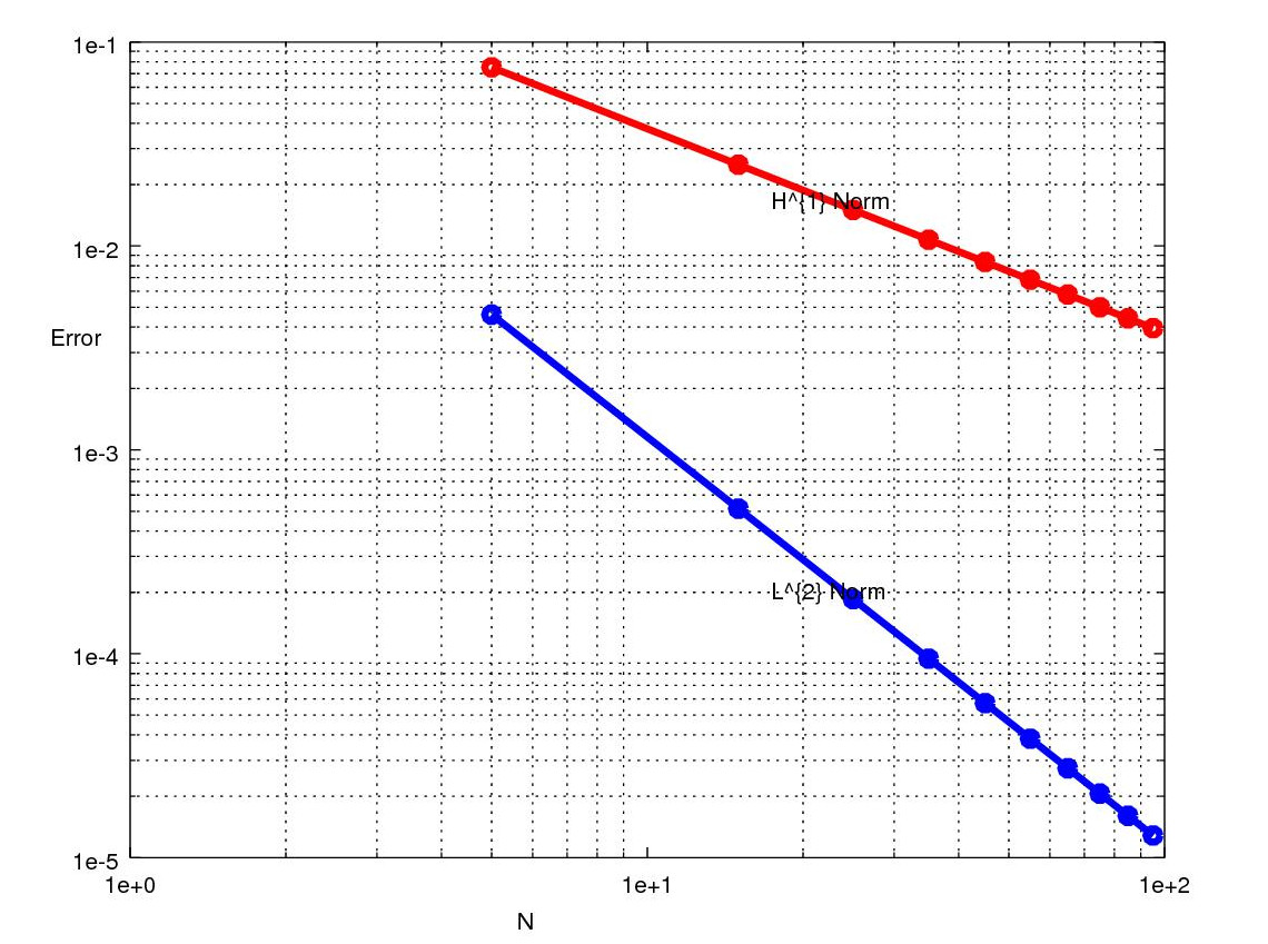
Figure 4: $L^{2}$ (in blue line) and $H^{1}$ (in red line) error $\lVert u-u_{h}\rVert$ plot

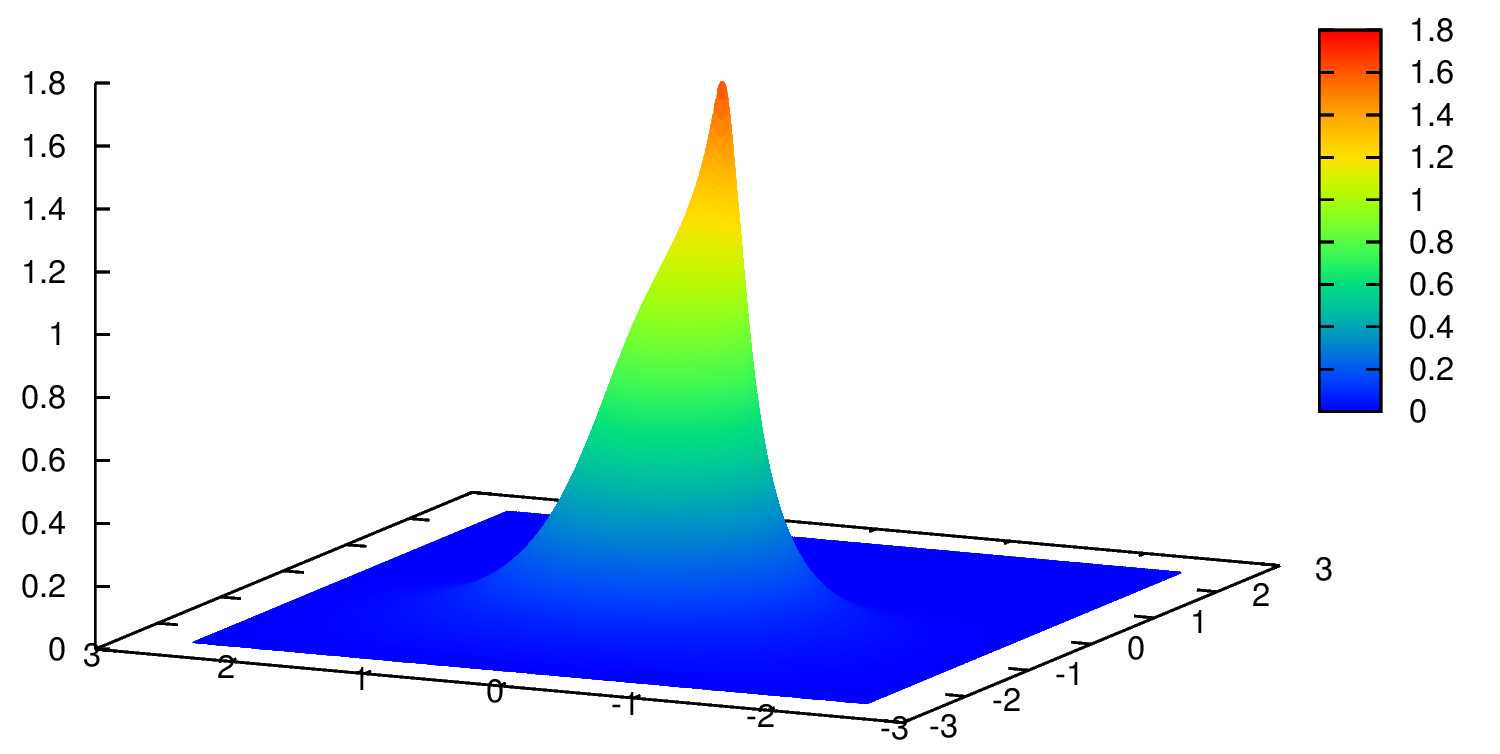
Figure 5: Pressure profile for light load case $M=7$ and $L=10$ (Moe’s parameter)

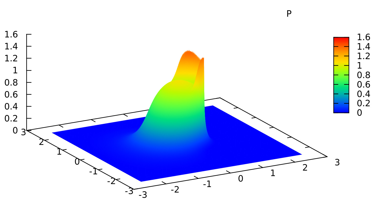
Figure 6: Pressure profile for moderately high load case $M=20$ and $L=10$

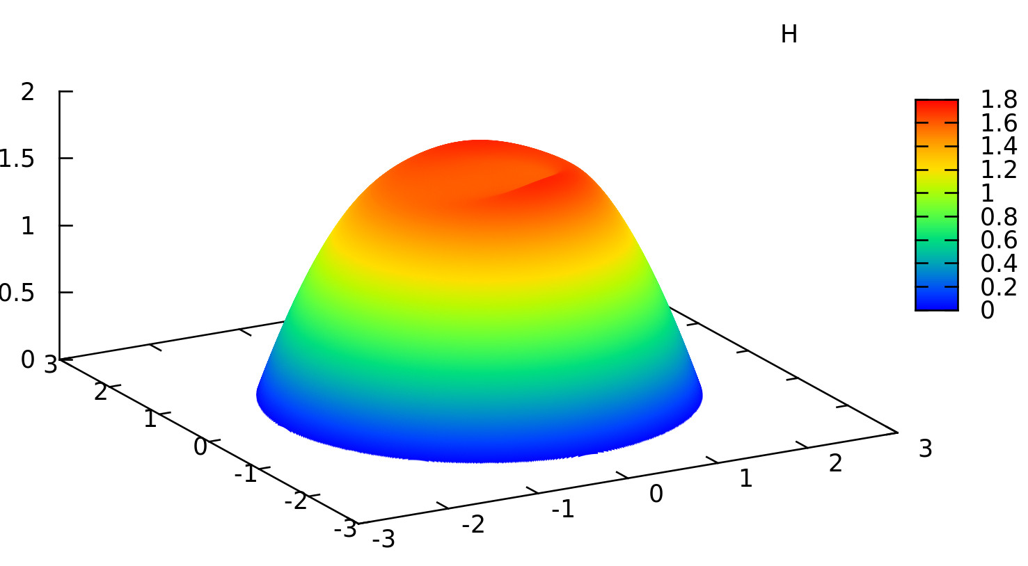
Figure 7: Film thickness profile in inverted form for $M=20$ and $L=10$

5.1 Film thickness calculation

Accurate film thickness $H$ computation is very important for stable relaxation procedure and require extra care in its computation. Film thickness calculation is calculated as follows

$${h_{d}(x,y)}={h_{0}+\frac{{x}^{2}+{y}^{2}}{2}+\frac{2}{\pi^{2}}\int_{x_{-}}^{x_{+}}\int_{y_{-}}^{y_{+}}\frac{p(x^{\prime},y^{\prime})dx^{\prime}dy^{\prime}}{\sqrt{(x-x^{\prime})^{2}+(y-y^{\prime})^{2}}}}$$ (124)

$$=h_{0}+\frac{{x}^{2}+{y}^{2}}{2}+\frac{2}{\pi^{2}}\sum^{N}_{e=1}\int_{e}\frac{\sum^{p_{e}+1}_{i=0}a^{e}_{i}\mathscr{N}^{e}_{i}(x^{\prime},y^{\prime})}{\sqrt{(x-y^{\prime})^{2}+(y-y^{\prime})^{2}}}dx^{\prime}dy^{\prime}$$ (125)

$$=h_{0}+\frac{{x}^{2}+y^{2}}{2}+\frac{2}{\pi^{2}}\sum^{N}_{e=1}\sum^{p_{e}+1}_{i=0}\int_{e}\frac{a^{e}_{i}\mathscr{N}^{e}_{i}(x^{\prime},y^{\prime})dx^{\prime}dy^{\prime}}{\sqrt{(x-y^{\prime})^{2}+(y-y^{\prime})^{2}}}$$ (126)

$$=h_{0}+\frac{{x}^{2}+y^{2}}{2}+\frac{2}{\pi^{2}}\sum^{N}_{e=1}\sum^{p_{e}+1}_{i=0}\mathscr{G}^{e}_{i}(x,y)a^{e}_{i}$$ (127)

5.2 Mild singular integral computation

Singularity at $(x^{\prime},y^{\prime})=(x,y)$ can be approximated in the following manner. We first rewrite kernel $\mathscr{G}^{e}_{i}(x)$ in the following form

$$\mathscr{G}^{e}_{i}(x)=\int_{\Omega_{e}}\frac{\mathscr{N}^{e}_{i}(x^{\prime},y^{\prime})dx^{\prime}dy^{\prime}}{\sqrt{(x-y^{\prime})^{2}+(y-y^{\prime})^{2}}}$$

$$=\frac{h_{x}^{e}}{2}\frac{h_{y}^{e}}{2}\int_{-1}^{1}\int_{-1}^{1}\frac{\mathscr{N}^{e}_{i}(x^{\prime}(\xi,\chi),y^{\prime}(\xi,\chi))d\xi d\chi}{\sqrt{(x-x^{\prime}(\xi,\chi))^{2}+(y-y^{\prime}(\xi,\chi))^{2}}}$$

$$\approx\frac{h_{x}^{e}}{2}\frac{h_{y}^{e}}{2}\sum_{j=1}^{m}\sum_{k=1}^{m}\frac{\mathscr{N}^{e}_{i}(x^{\prime}(\xi_{j},\chi_{k}),y^{\prime}(\xi_{j},\chi_{k}))w_{j}w_{k}}{\sqrt{(x-x^{\prime}(\xi_{j},\chi_{k}))^{2}+(y-y^{\prime}(\xi_{j},\chi_{k}))^{2}}},$$ (128)

where $h_{x}^{e}=x_{2}-x_{1}$ and $h_{y}^{e}=y_{2}-y_{1}$ are the step sizes of element $e$ in the $x$ direction and $y$ direction respectively and $\xi\in[-1,1]$ and $\chi\in[-1,1]$ are the coordinate directions for the reference element. We have applied here $m$ point quadrature in $x$ and $y$ direction of discretization. Singular quadrature procedure is implemented here to resolve the singularity appeared in term $\mathscr{G}_{i}^{e}(x,y)=\frac{1}{\sqrt{(x-x^{\prime})^{2}+(y-y^{\prime})^{2}}}$ at the point $(x,y)$. Idea involve by dividing the element $e$ into four subpart elements $\mathscr{F}_{k},k=1,2,3,4$ for calculating integrals of $\mathscr{G}_{i}^{{\mathscr{F}_{k}}}(x,y)=\frac{1}{\sqrt{(x-x^{\prime})^{2}+(y-y^{\prime})^{2}}}$. Each four integrals have chosen in a such way that they have only one singular point in the domain of integration. Four integrals defined above can be evaluated as in general integral form:

$$\mathscr{S}^{*}=\int_{0}^{1}\int_{0}^{1}\mathscr{F}^{*}(x,y)\mathscr{G}^{*}(x,y)dxdy,$$ (129)

where $\mathscr{F}^{*}$ is analytic function and $\mathscr{G}^{*}$ is a function having a mild singularity at only one point.

$$\mathscr{S}\approx\mathscr{S}_{n}^{*}=\sum_{i=1}^{n}\mathscr{I}_{i},$$ (130)

where

$$\mathscr{I}_{i}=\int_{x_{i}}^{x_{i-1}}\int_{y_{i}}^{y_{i-1}}\mathscr{F}^{*}(x,y)\mathscr{G}^{*}(x,y)dxdy,(i\geq 1).$$ (131)

Where $(x_{0},y_{0})=(1,1)$ and $(x_{n},y_{n})\rightarrow(0,0)\quad\text{as}\quad n\rightarrow\infty$ for the value $(x_{n},y_{n})=(\theta^{n},\theta^{n}),(0<\theta<1)$.

5.3 Load balance equation calculation

The force balance equation is discretized according to:

$$\sum^{N}_{e=1}\int_{\Omega_{e}}\sum^{p_{e}+1}_{i=0}{\mathscr{G}_{1}}^{e}_{i}(x,y)a^{e}_{i}dxdy-\frac{2\pi}{3}=0$$ (132)

By introducing another kernel $\mathscr{N_{1}}^{e}_{i}$

$${\mathscr{G}_{1}}^{e}_{i}=\int_{\Omega_{e}}\mathscr{N_{1}}^{e}_{i}(x,y)dxdy$$ (133)

the discrete force balance equation can be rewritten as:

$$\sum^{N}_{e=1}\sum^{p_{e}+1}_{i=0}(\mathscr{N_{1}}^{e}_{i})a^{e}_{i}-\frac{2\pi}{3}=0$$ (134)

6 Conclusion

New discontinuous Galerkin finite volume method is developed and analyzed with the help of interior-exterior penalty approach. The method is fully systematic and easily parallelized in MPI (Massage passing interface) environment. Stability estimates are proved by showing operator as pseudo-monotone for moderate load condition. Optimal error estimates are achieved under light load condition theoretically as well as by numerical computation in $H^{1}$ and $L^{2}$ norm respectively. More implementation issues and applications will be discussed in the second part of the paper.

Appendix A Relaxation of EHL

For finding unique solution we can update our nonlinear operator iterative manner by taking old and new pressure value in the following form

$$U_{\text{new}}=U_{\text{old}}+\Big{(}\frac{\partial\mathscr{T}_{d}(U)}{\partial U}\Big{)}^{-1}\mathcal{R}_{s},$$ (135)

where $\mathcal{R}_{s}$ is the numerical residual value of the discretized Reynolds equation and, $\mathscr{T}_{d}$ is discretized nonlinear operator. The approximation of $\frac{\partial\mathscr{T}_{d}(U)}{\partial U}$ can be evaluated in the following way,

$$\frac{\partial\mathscr{T}_{d}(U)}{\partial U}\approx\frac{\partial\mathscr{T}^{*}_{d}(U)}{\partial U}-\frac{\partial\mathscr{T}^{**}_{d}(U)}{\partial U}$$

$$\approx\mathscr{A}^{*}_{d}(U)-\frac{\partial\mathscr{T}^{**}_{d}(U)}{\partial U}$$ (136)

In the above equation 136, we can notice that term $\frac{\partial\mathscr{T}^{**}_{d}(U)}{\partial U}$ is a full dense matrix and evaluated in the following way,

$$\frac{\partial\mathscr{T}^{**}_{d}(U)}{\partial U}\Big{|}_{I,J}=\sum\limits_{K\in\mathscr{R}_{h}}\sum\limits_{j=1}^{3}\int_{A_{j+1}CA_{j}}(\rho\frac{\partial h_{d}}{\partial U_{j}^{f}}+h_{d}\frac{\partial\rho}{\partial U_{j}^{f}}).(\beta.\mathbb{n})\gamma vds$$

$$+\sum\limits_{e\in\Gamma}\int_{e}[\gamma v]\Big{\{}(\rho\frac{\partial h_{d}}{\partial U_{j}^{f}}+h_{d}\frac{\partial\rho}{\partial U_{j}^{f}}).(\beta.\mathbb{n})\Big{\}}ds,$$

where the $I^{\text{th}}$ subscript denote the row generated with the test function $v=\mathscr{N}^{e}_{i}(\mathbb{X})$ and the $J^{\text{th}}$ subscript correspond to the unknown $U_{j}^{{\mathscr{F}}}$. According to the equation (60) we can evaluate the following expression

$$\frac{\partial h_{d}}{\partial U_{j}^{f}}=\mathscr{G}_{j}^{f}$$

which can be pre-evaluated. It is worth mentioning that, from equation (60) the film thickness depends heavily on the local pressure and very less on the pressure for away. The value of $\mathscr{G}_{j}^{{\mathscr{F}}}$ is rapidly decreases as the position of element $\mathscr{F}$ is far away from the position of $\mathbb{X}=(x,y)$. From the above information we can reduce our computation cost by considering the following approximations of $\frac{\partial\mathscr{T}^{**}_{d}(U)}{\partial U}$:

• $\frac{\partial h_{d}(\mathbb{X})}{\partial U_{j}^{f}}=0$ where $\mathbb{X}\in e$ if $f\neq e$ and $f$ is not a adjacent element of $e$.

• $\frac{\partial h_{d}(\mathbb{X})}{\partial U_{j}^{f}}=0$ where $\mathbb{X}\in\Gamma_{\text{int}}$ and if $f$ is not a adjacent element of $\Gamma_{\text{int}}$.

• $\frac{\partial h_{d}(\mathbb{X})}{\partial U_{j}^{f}}=0$ where $\mathbb{X}\in\Gamma_{D}$ and if $f$ is not a adjacent element of $\Gamma_{D}$.

• $\frac{\partial h_{d}(\mathbb{X})}{\partial U_{j}^{f}}=\mathscr{G}_{j}^{f}(\mathbb{X})$, otherwise.

Appendix B Parameters used in computation

Following Parameters relation is defined in our study for $\epsilon^{*},\rho(u),\eta(u),\lambda.$

$$\rho(u)=\rho_{0}\frac{l_{1}+1.34u}{l_{1}+u}$$

$$\eta(u)=\eta_{0}e^{l_{2}u}$$

$$\epsilon^{*}=\frac{\rho h^{3}_{d}}{\eta\lambda}$$

$$\lambda=\frac{12\mu v(2R)^{3}}{\pi E}$$ (137)

where $l_{1}=0.59\times 10^{9}$ and $l_{2}\approx 2.0\times 10^{-8}$.

References

- [1] D. N. Arnold. An interior penalty finite element method with discontinuous elements. SIAM J. Numer. Anal., 15(1):742–760, 1982.
- [2] J. Aubin. Approximation des problemes aux limites non homogeneous pour des operatoeurs non linearires. J. Math. Anal. Appl., 30(7):510–521, 1970.
- [3] M.F. Wheeler B. Riviére and V. Girault. A priori error estimates for finite element methods based on discontinuous approximation spaces for elliptic problems. SIAM J Numer Anal, 39(1):901–931, 2001.
- [4] I. Babuška. The finite element method with penalty. Math. Comp., 27(1):221–228, 1976.
- [5] S. Chou and X. Ye. Unified analysis of finite volume methods for second order elliptic problems. SIAM J. Numer. Anal., 45(4):1639–1653, 2007.
- [6] S. H. Chou. Analysis and convergence of a covolume method for the generalized stokes problem. Math Com., 66(1):85–104, 1997.
- [7] S. H. Chou and D. Y. Kwak. Analysis and convergence of a mac scheme for generlized stoke problem. Num.Methods PDE, 13(1):147–162, 1997.
- [8] J. Douglas. and T. Dupont. Interior penalty procedures for elliptic and parabolic galerkin methods in computing in applied science. Lecture Notes in Physics, 58(1):207–216, 1976.
- [9] Oden J. T and S. R. Wu. Existence of solutions to the reynolds equation of elastohydrodynamic lubrication. Int. J. Engng Sci., 23(2):207–215, 1985.
- [10] R. D. Lazarov, I. D. Mishev, and P. S. Vassilevski. Finite volume methods for convection-diffusion problems. SIAM J. Numer. Anal., 33(1):33–55, 1996.
- [11] J. L. Lions. Problems aus limites non homogenes a donees irregulieres. Une mathode d’approximation, in Numeri. Anal. of PDE, 1(1):283–292, 1968.
- [12] H. Moes. Optimum similarity analysis with applications to elastohydrodynamic lubrication. Wear, 159(1):57–66, 1992.
- [13] J. A. Nitsche. Uber ein variationsprinzip zur losung dirichlet-problemen bei verwendung von teilraumen, die keinen randbedingungen unteworfen sind. Abh. Math. Sem. Univ. Hamburg, 36(1):9–15, 1971.
- [14] C. Ortner and E. Suli. Discontinuous galerkin finite element approximation of nonlinear second order elliptic and hyperbolic systems. SIAM J. Numer. Anal., 45(4):1370–1397, 2007.
- [15] M. F. Wheeler. An elliptic collocation-finite element method with interior penalties. SIAM J. Numer. Anal., 15(1):152–161, 1978.
- [16] X. Ye. A new discontinuous finite volume method elliptic problems. SIAM J. Numer. Anal., 42(3):1062–1072, 2004.