Cosmographic analysis with Chebyshev polynomials
Abstract
The limits of standard cosmography are here revised addressing the problem of error propagation during statistical analyses. To do so, we propose the use of Chebyshev polynomials to parameterize cosmic distances. In particular, we demonstrate that building up rational Chebyshev polynomials significantly reduces error propagations with respect to standard Taylor series. This technique provides unbiased estimations of the cosmographic parameters and performs significatively better than previous numerical approximations. To figure this out, we compare rational Chebyshev polynomials with Padé series. In addition, we theoretically evaluate the convergence radius of (1,1) Chebyshev rational polynomial and we compare it with the convergence radii of Taylor and Padé approximations. We thus focus on regions in which convergence of Chebyshev rational functions is better than standard approaches. With this recipe, as high-redshift data are employed, rational Chebyshev polynomials remain highly stable and enable one to derive highly accurate analytical approximations of Hubble’s rate in terms of the cosmographic series. Finally, we check our theoretical predictions by setting bounds on cosmographic parameters through Monte Carlo integration techniques, based on the Metropolis-Hastings algorithm. We apply our technique to high-redshift cosmic data, using the JLA supernovae sample and the most recent versions of Hubble parameter and baryon acoustic oscillation measurements. We find that cosmography with Taylor series fails to be predictive with the aforementioned data sets, while turns out to be much more stable using the Chebyshev approach.
I Introduction
The cosmic acceleration is today confirmed by a large number of observations Riess98 ; Perlmutter99 and represents a consolidate challenge of modern cosmology. To disclose the physics behind it, model-independent techniques have been widely investigated during last years. Strategies toward model-independent treatments have as main target the determination of universe’s expansion history without the need of postulating a priori dark energy contributions. A particular attention is currently given to cosmography Visser04 ; Cattoen07 ; Saini00 ; Cai11 ; Guimaraes11 ; Arabsalmani11 ; Carvalho11 ; Luongo11 ; Capozziello11 . Standard cosmography lies on Taylor expansions of cosmic distances. The method provides a powerful tool to study the dark energy evolution without assuming its functional form in the Hubble rate. Moreover, fixing limits over free cosmographic parameters alleviates degeneracy among models and enables to understand which paradigms are effectively favored directly with respect to data surveys. Although cosmography candidates as a robust tool to understand whether dark energy evolves or not, cosmic data unfortunately span on intervals . This limit poses severe restrictions on cosmography and makes inapplicable Taylor expansions built up around .
One stratagem to overcome this problem is to parameterize Taylor expansions in terms of auxiliary variables. Unfortunately, even this case turns out to be jeopardized by severe error propagations over the final outcomes. More recently, a further effort has been the use of Padé approximation built up to converge at higher redshift domains Gruber14 ; Wei14 . In this case, however, the expansion orders are not fixed a priori and this causes difficulties on evaluating the rate of convergence as . Thus, the limits of standard Taylor approach lying on are essentially alleviated but not fully fixed.
Motivated by the need of reducing relative uncertainties in cosmography, we here propose a new cosmographic technique based on Chebyshev polynomials. Chebyshev polynomials represent sequences of orthogonal polynomials, recursively-defined through trigonometric functions. In our approach we develop a new Chebyshev cosmography adopting the strategy of building up rational approximations made by these polynomial functions. We demonstrate that, under the hypothesis of rational Chebyshev polynomials, distinguishing Chebyshev functions of first and second kinds is not relevant since the final output gives analogous results in both the cases. For simplicity, we limit our analysis on first kind Chebyshev polynomials only and we write the sequence of Chebyshev rational functions which better approximate Taylor series up to a certain order. We thus show that our Chebyshev ratios provide nodes in polynomial interpolation, minimizing cosmographic uncertainties leading to the most likely well-motivated approximation to cosmic distances. We even present theoretical motivations behind our choice by computing the convergence radii for different choices of polynomial approximations.
To check how well our model works we also study Padé expansions and we compare the Chebyshev technique with them. We finally show the advantages of our procedure with respect to the old approaches using data surveys, confronting the cosmological quantities built from our method with the observables of the latest cosmological data sets. We adopt a Monte Carlo analysis employing the Metropolis-Hastings algorithm, choosing JLA supernova, baryon acoustic oscillation and differential age measurements. We show the goodness of our procedures comparing the outcomes coming from standard cosmography and our method, showing that error uncertainties are effectively reduced.
The structure of the paper is as follows. In Sec. II, we review the general aspects of cosmography. In Sec. III, we describe the mathematical features of the Chebyshev polynomials and present the method of the rational Chebyshev approximations. In Sec. IV, we derive a new model-independent formula for the luminosity distance, and compare the new method with the standard cosmographic procedures to verify the goodness of our approach. In Sec. V, we place observational limits on the cosmographic parameters through a confront with the most recent experimental data. Finally, in Sec. VI we summarize our findings and conclude.
II The cosmographic approach
The study of the cosmic evolution can be done independently of energy densities by means of cosmography. This model-independent technique only relies on the observationally justifiable assumptions of homogeneity and isotropy Weinberg72 ; Visser97 ; Harrison76 . The great advantage of this method is that it allows one to reconstruct the dynamical evolution of the dark energy term without assuming any particular cosmological model. Cosmography involves Taylor expansions of observable quantities that may, in principle, go up to any order. These expansions can be compared directly with data. The outcomes of this procedure ensure the independence from any postulated equation of state governing the evolution of the universe and, thus, help to break the degeneracy among cosmological models.
The homogenous and isotropic universe is governed by the single degree of freedom offered by , as demanded by the cosmological principle. Hence, following the most recent measurements of Planck15 and assuming a spatially flat universe111The assumption of flatness overcomes problems of degeneracy among the cosmographic parameters entering the expression of the luminosity distance Dunsby16 ., we can expand in Taylor series around present time Visser05 ; Visser15 :
| (1) |
where .
The expansion above defines the cosmographic series Poplawski06 ; Poplawski07 ; Cattoen08 ; Xu11 ; Aviles12 :
| (2) | |||
| (3) |
known in the literature as Hubble, deceleration, jerk and snap parameters222In principle, one may go further in the expansion and consider higher order coefficients. We limit our study up to the snap, since the next cosmographic parameters are poorly constrained by observations Aviles12 .. These coefficients are used to describe the expansion history of the universe at late times.
Using the relation and Eq. 1, one finds the Taylor series expansion of the luminosity distance as function of the redshift Busti15 ; Demianski12 ; Piedipalumbo15 ; Demianski17 :
| (4) |
The above expression for the luminosity distance can be used to obtain limits on the cosmographic parameters and study the low- dynamics of the universe with no need of any a priori assumed cosmological model. In fact, plugging Eq. 4 into the definition
| (5) |
one gets
| (6a) | ||||
| (6b) | ||||
| (6c) | ||||
| (6d) | ||||
which describes the expansion history of the late-time universe up to the snap parameter.
II.1 The convergence problem
The limits of the standard cosmographic approach, based on the Taylor approximations, emerge when cosmological data at high redshifts are used to get information on the evolution of the dark energy term. In fact, the Taylor series converges if , so that any cosmographic analysis employing data beyond this limit is plagued by severe restrictions. A way to extend the radius of convergence of the Taylor series to high-redshift domains is represented by the method of rational approximations, among which the Padé polynomials represent a relevant example Baker96 . The Taylor expansion of a generic function is , where , whereas one defines the Padé approximant of as the rational polynomial
| (7) |
Since by construction one requires that , we have:
| (8) |
The coefficients in Eq. 7 are thus determined by solving the following homogeneous system of linear equations Litvinov93 :
| (9) |
valid for . All coefficients in Eq. 7 may be computed using the formula
| (10) |
The technique of Padé approximations has been recently investigated in the context of cosmography to handle the divergence problems at high- domains Gruber14 ; Wei14 . In the next section, we present the method of rational Chebyshev polynomials that we will use to obtain a new cosmographic expression for the luminosity distance.
III Rational Chebyshev polynomials
The method we propose here aims to optimize the technique of rational polynomials and consists of approximating the luminosity distance with a ratio of Chebyshev polynomials. In fact, the Padé approximants are built up from the Taylor approximation of whose error bars, by construction, rapidly increase as the redshift departs from zero. Motivated by this issue, we exploit the Chebyshev polynomials. Such a choice aims at reducing the uncertainties on the estimate of the cosmographic parameters.
The Chebyshev polynomials333Throughout the text, we refer to the Chebyshev polynomials of the first kind simply as Chebyshev polynomials. are defined through the identity
| (11) |
where and . They form an orthogonal set with respect to the weighting function in the domain Chebyshev :
| (12) |
where is the Kronecker delta. The Chebyshev polynomials are generated from the recurrence relation
| (13) |
The explicit expressions of the first five polynomials444We here truncate our analysis to the fifth order, since additional contributions go beyond our treatment. In so doing, we arrive to analyse up to snap parameter . that we will employ to build the new expression for read numerical :
| (14) | ||||
It is possible to express the powers of in terms of the Chebyshev polynomials according to the formula Litvinov93 :
| (15) |
for . Here, is the integer part of , if and if , and are the binomial coefficients.
Let , being the Hilbert space of the square-integrable functions with respect to the measure . Suppose we know the truncated Taylor series of around the point , . It is possible to obtain the polynomial of degree , ,which gives the best approximation of in the interval in . Formally, the Chebyshev series expansion of reads
| (16) |
where
| (17) |
Hence, we define the rational Chebyshev approximant as
| (18) |
For , through a redefinition of the coefficients, we can recast Eq. 18 in the form
| (19) |
Applying a similar procedure used to obtain the Padé approximants, one can calculate the unknown coefficients and by equating Eq. 16 and Eq. 19 up to the -th Chebyshev polynomial:
| (20) |
By doing so, one gets:
| (21) |
To calculate the products of Chebyshev polynomials that occur in the left hand side of Eq. 21, one can make use of the trigonometric identity
which leads to the relation
| (22) |
Thus, equating the terms with the same degree of ’s yields equations for the unknowns in Eq. 19.
In the next section, we apply the mathematical procedure we have presented above to find a very accurate model-independent expression for the luminosity distance. We also compare our method with the cosmographic approaches developed so far in the literature.
IV The Chebyshev cosmography
We are here interested in approximating the luminosity distance with rational Chebyshev polynomials. First, we need to express in terms of Chebyshev polynomials according to Eq. 16. To do that, we calculate the coefficients in Eq. 17 where, in our case, is the Taylor expansion given in Eq. 4. Hence, the fourth-order Chebyshev expansion of the luminosity distance can be expressed as
| (23) |
where the coefficients read:
Thus, one can construct the rational Chebyshev approximations of as in Eq. 19 starting from Eq. 23. We report some explicit expressions in Appendix A. Polynomials of high degrees will lead to more accurate approximations, even though these are the ones characterized by more complicated analytical forms, of course.
IV.1 Calibrating Chebyshev polynomials with the concordance model
To check the accuracy of various Chebyshev approximations, we compare them with the CDM luminosity distance, :
| (24) |
in which we have:
| (25) |
According to a spatially flat universe, we set , having the matter density at current time. In the concordance paradigm case, the cosmographic parameters can be calculated in terms of :
| (26) | ||||
As an indicative possibility, we fix . So that from Eq. 26 one gets:
| (27) |
Using the values of Eq. 27, in Fig. 1 we show the behaviour with the redshift of for different degrees of rational Chebyshev approximations.
In principle, to approximate the CDM model some of the rational Chebyshev polynomials may present singularities turning out to give unsuitable outcomes. To overcome this issue, the preferred rational approximations are those with , in analogy to what happens for Padé approximations Aviles14 . In particular, as practically checked the approximant seems to give the most accurate approximation to the luminosity distance of the CDM model. Assuming that the calibration with the concordance paradigm would be viable for any possible dark energy term, we assume that the most suitable approximation with Chebyshev polynomials comes from .
To portray a qualitative representation of numerical improvements that one gains using our method, we compare with the standard fourth-order Taylor expansion of given in Eq. 4, and with the (2,2) Padé approximation of . We choose the (2,2) Padé approximation since it has been argued that it is robustly characterized by good convergence properties Aviles14 as used in computational analyses. We note that, while in the Taylor and Padé approximations the snap parameter shows up at the fourth order, in the rational Chebyshev polynomials it is present from the lowest degrees, since all the coefficients of Eq. 23 have been calculated from the Taylor series expansion of up to the snap order (as confirmed in Eq. 4). For comparison, we report the expression of the (2,2) Padé approximation of in Appendix B. In Fig. 2, we show the behaviour of for the various techniques. As can be seen, the Taylor approach fails when . Our Chebyshev cosmography stands out for the excellent approximation to the CDM luminosity distance, resulting mostly more effective than Padé approximations.
IV.2 The convergence radius
We here argue how to broadcast the above considerations to well-motivated theoretical scenarios. Thus, we wonder whether Chebyshev cosmography is expected to effectively improve the approximations to cosmic distances than standard cosmography. To do so, it behooves us to check how much the aforementioned approximations are stable to higher redshifts. Hence, one can test the ability of the various cosmographic techniques, able to describe high-redshift domains, by a direct comparison among the corresponding convergence radii, here defined by .
As a simple example, we explicitly calculate the convergence radius of the (1,1) rational Chebyshev approximation of the luminosity distance, compared to the second-order Taylor series and to the (1,1) Padé approximation. From Eqs. 19 and 14, it holds
| (28) |
where the coefficients are expressed in terms of the cosmographic series as shown in Eq. 44. We can rearrange Eq. 28 as
| (29) |
and, after some algebra, one obtains
| (30) |
The geometric series in Eq. 30 converges for , so that the convergence radius of the (1,1) rational Chebyshev approximation of is
| (31) |
Analogous calculations show that the convergence radius of the (1,1) Padé approximant for is
| (32) |
The convergence radius of the second-order Taylor series of is approximately given by
| (33) |
For the sake of completeness, the numerical values of and should be computed by using fitting results over the cosmographic coefficients. However, an analogous check can be made assuming the reference values Eq. 26. In such a case, one gets:
| (34) |
These indicative results confirm the improvements of the rational polynomials in extending the radius of convergence with respect to the Taylor series. From the outcomes of Eq. 26 we notice that the convergence radius of the Padé approximation seems fairly better than the Chebyshev one. However, this is due to the choice made on the set and . In Fig. 3 we plot the convergence radii for Taylor, Padé and Chebyshev polynomials with a different set of cosmographic coefficients not calibrated over the concordance paradigm. In Fig. 3, in particular, we show the regions in which the improvements of Chebyshev rational approximations become significant in terms of the convergence radius.
V Observational constraints
In this section, we present the data we use to set bounds on the cosmographic parameters.
V.1 Supernovae Ia
In the present work, we test the Joint Light-curve Analysis (JLA) sample of 740 SNe of type Ia Betoule14 in the redshift interval . All the SNe have been standardized using the SALT2 model Guy07 as fitter for their light curves. The catalogue provides, for each SN, the redshift , model-independent apparent magnitude in the band , the stretch factor of the light-curve , and the colour at maximum brightness . The theoretical distance modulus,
| (35) |
is parametrized as follows:
| (36) |
where the absolute magnitude is defined as
| (37) |
being the host stellar mass. The nuisance parameters {, , , } are fitted together with the cosmological parameters. The normalized likelihood function of the SNe data is given by
| (38) |
where C is the covariance matrix constructed as in Betoule14 , which includes statistical and systematic uncertainties on the light-curve parameters.
V.2 Observational Hubble Data
The Hubble rate of a given cosmological model can be constrained by means of the model-independent measurements acquired through the differential age (DA) method, first presented in Jimenez02 . Such a technique uses red passively evolving galaxies as cosmic chronometers. In particular, one can obtain by measuring the age difference of two close galaxies and using the relation:
| (39) |
The normalized likelihood function for the OHD data is built using a collection of 31 uncorrelated DA measurements of , which we report in Appendix C:
| (40) |
V.3 Baryon Acoustic Oscillations
Intensive studies on the large scale structures of the universe have been done thanks to galaxy surveys. The baryon acoustic oscillations that occur in the relativistic plasma come in the form of a characteristic peak in the galaxy correlation function. The BAO measurements are usually given in the literature as , namely the ratio between the comoving sound horizon at the drag epoch and the spherically averaged distance measure introduced in Eisenstein05 :
| (41) |
We construct the normalized likelihood function for the BAO data using the six uncorrelated and model-independent measurements given in Lukovic16 , which we list in Appendix C:
| (42) |
V.4 Results of the Monte Carlo analysis
To test the different cosmographic approaches, we performed a Markov Chain Monte Carlo (MCMC) integration on the combined likelihood of the datasets we presented above:
| (43) |
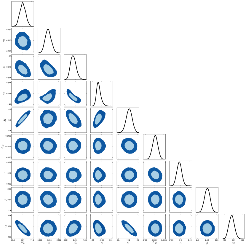
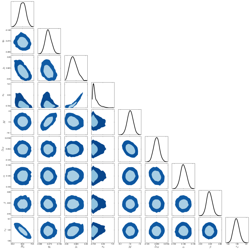
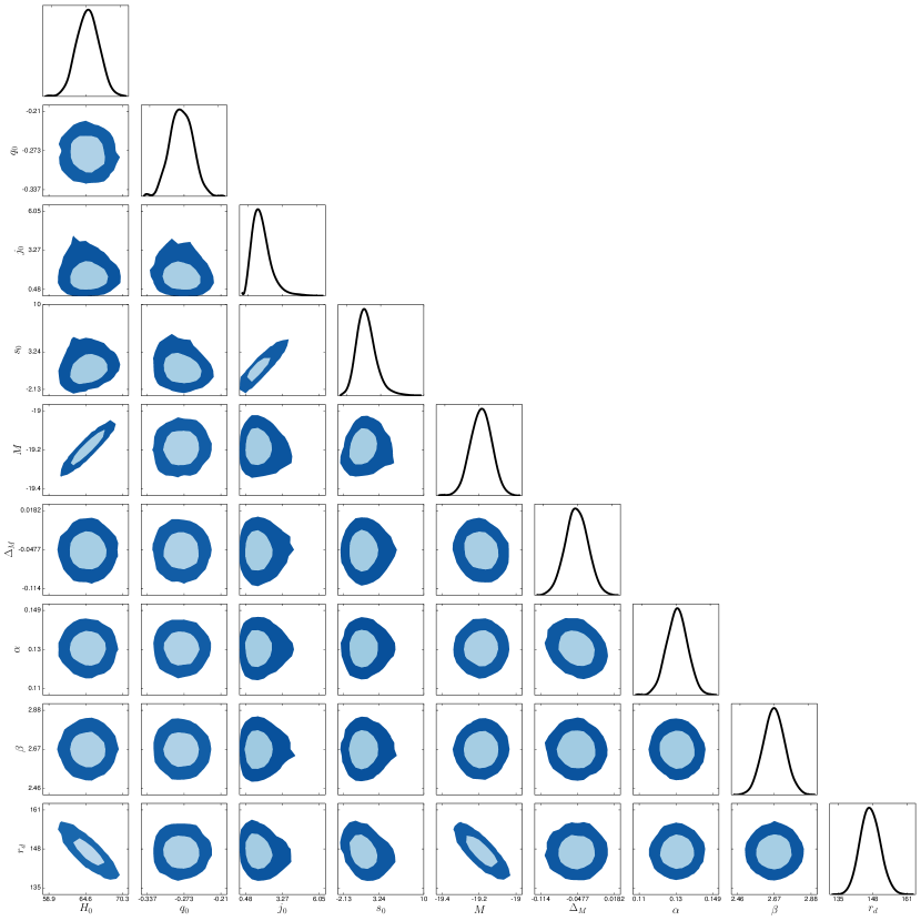
We implemented the Metropolis-Hastings algorithm with the Monte Python code MontePython , assuming uniform priors for the parameters (see Table 1). The numerical results of our joint analysis are shown in Table 2. Also, in Figs. 4, 5 and 6 we show the marginalized 2D and regions and the 1D posterior distributions for the cosmological and nuisance parameters in the case of the three cosmographic techniques. Our results prove that the method of rational Chebyshev polynomials reduces the uncertainties in the estimate of the cosmographic parameters with respect to the other approaches, as shown by the relative errors in Table 3.
An alternative approach is to start from the cosmographic expansion series of the Hubble rate and, then, evaluate the luminosity distance by numerical integrations, as pointed out in Aviles17 . However, it turns out that the analysis based on rational Chebyshev approximations of does not lead to further reduction of the error propagation with respect to our original approach.
| Parameters | Priors |
|---|---|
| Parameter | Taylor | Padé | Rational Chebyshev | ||||||
|---|---|---|---|---|---|---|---|---|---|
| Mean | Mean | Mean | |||||||
| Parameter | Taylor | Padé | Rational Chebyshev | |||
|---|---|---|---|---|---|---|
VI Summary and conclusions
In this work, we revised the convergence problem in cosmography, adopting a new method to reduce error uncertainties and bias propagations as high-redshift data are used. We set bounds on the cosmographic series, considering rational approximations of the luminosity distance and we demonstrated that such approximations are also valid for any cosmic distances. In particular, our novel procedure is based on approximating the luminosity distance with ratios of Chebyshev polynomials. Since, by definition, Chebyshev approximants are the most suitable polynomials in approximating functions, we expected to get fairly good outcomes in computing cosmographic series. Indeed, we found that our approach overcomes the convergence issues typical of standard cosmographic techniques based on Taylor approximations. This has been confirmed by computing convergence radii for different sets of cosmographic coefficients. We also compared our new approach with the consolidate procedure of Padé expansions. We showed that both numerical bounds and convergence radii are improved under precise conditions. This naturally showed that Chebyshev rational polynomials are more suitable to describe the cosmic dynamics at than Padé series. Bearing this in mind, through the predictions of the concordance CDM model, we calibrated the orders of Chebyshev rational polynomials, providing the recipe of a new Chebyshev cosmography, which turned out to be more predictive than Taylor series at all redshift domains. We evaluated the (2,1) Chebyshev series, corresponding to a fourth-order Tayor series and to a (2,2) Padé approximation. This showed that lower order Chebyshev series work better than higher ones constructed by Taylor and Padé recipes. We finally checked the goodness of our method, statistically combining the JLA supernova compilation, differential age data and baryon acoustic oscillation measurements by performing Monte Carlo integrations based on the Metropolis-Hastings algorithm. To do so, we employed the free available Monte Python code and we computed the corresponding contours up to the confidence level. The numerical improvements have been reported in terms of percentages on 1 and 2 confidence levels. The error percentages are severely lowered whereas the mean values are centred around intervals compatible with previous results on cosmography.
Our final outcomes forecast that the technique of Chebyshev cosmography substantially decreases the relative uncertainties on the estimates of cosmographic parameters respect to other previous approaches. This procedure candidates as a new way toward computing the cosmographic series and to better fix constraints on cosmography. Chebyshev cosmography is thus able to heal previous inconsistencies on convergence which plagued cosmography itself. Further, it enables to use high-redshift data surveys in cosmographic analyses with no large spreads over fitted coefficients.
Future efforts will be devoted to match Padé and Chebyshev techniques in different redshift domains. We will work on characterizing the cosmographic data over binning intervals in which one will be able to highly maximize both the convergence radii and mean values and to minimize both bias and uncertainties on free cosmographic coefficients.
Acknowledgements
This paper is based upon work from COST action CA15117 (CANTATA), supported by COST (European Cooperation in Science and Technology). S.C. acknowledges the support of INFN (iniziativa specifica QGSKY). R.D. thanks Federico Tosone for useful discussions on the Monte Python code.
References
- (1) A. G. Riess et al., Astron. J., 116, 1009-1038, (1998).
- (2) S. Perlmutter et al., Astrophys. J., 517, 565-586 (1999).
- (3) P. A. R. Ade et al. [Planck Collaboration], Astron. Astrophys, 594, A13 (2016).
- (4) M. Visser, Classical Quantum Gravity 21, 2603 (2004).
- (5) C. Cattoen, M. Visser, Classical Quantum Gravity, 24, 5985 (2007).
- (6) T. D. Saini, S. Raychaudhury, V. Sahni, A. A. Starobinsky, Phys. Rev. Lett., 85, 1162 (2000).
- (7) R. Cai, Z. Tuo, Phys. Lett. B, 706, 116 (2011).
- (8) A. C. C. Guimaraes, J. A. S. Lima, Classical Quantum Gravity, 28, 125026 (2011).
- (9) M. Arabsalmani, V. Sahni, Phys. Rev. D, 83, 04350 (2011).
- (10) J. C. Carvalho, J. S. Alcaniz, Mon. Not. Roy. AstronSoc., 418, 1873-1877 (2011).
- (11) O. Luongo, Mod. Phys. Lett. A, 26, 1459 (2011).
- (12) S. Capozziello, R. Lazkoz, V. Salzano, Phys. Rev. D, 84, 124061 (2011).
- (13) C. Gruber, O. Luongo, Phys. Rev. D, 89, 103506 (2014).
- (14) H. Wei, X.-P. Yan, and Y.-N. Zhou, J. Cosmol. Astropart. Phys., 01 (2014).
- (15) S. Weinberg, Gravitation and Cosmology: Principles and Applications of the General Theory of Relativity, Wiley, Hoboken, NJ, USA, (1972).
- (16) M. Visser, Science, 276, 88 (1997).
- (17) E. R. Harrison, Nature, 260, 591 (1976).
- (18) P. K. S. Dunsby, O. Luongo, Int. J. Geom. Meth. Mod. Phys., 13, 1630002 (2016).
- (19) M. Visser, Gen. Rel. Grav., 37, 1541-1548 (2005).
- (20) M. Visser, Class. Quant. Grav., 32, 135007 (2015).
- (21) N. Poplawski, Phys. Lett. B, 640, 135 (2006).
- (22) N. Poplawski, Class. Quant. Grav., 24, 3013 (2007).
- (23) C. Cattoen, M. Visser, Phys. Rev. D, 78, 063501 (2008).
- (24) L. Xu, Y. Wang, Phys. Lett. B, 702, 114-120 (2011).
- (25) A. Aviles, C. Gruber, O. Luongo, H. Quevedo, Phys. Rev. D, 86, 123516 (2012).
- (26) V. C. Busti et al., Phys. Rev. D, 92, 123512 (2015).
- (27) M. Demianski et al., Mon. Not. Roy. Astron. Soc., 426, 1396 (2012).
- (28) E. Piedipalumbo et al., Intern. Jour. Mod. Phys. D, 24, 1550100 (2015).
- (29) M. Demianski et al., Astron. Astroph., 598, A113 (2017).
- (30) G. A. Baker Jr., P. Graves-Morris, Padé Approximants, Cambridge University Press (1996).
- (31) G. Litvinov, Appl. Russ. J. Math. Phys., 1(3), 313-352 (1993).
- (32) P. L. Chebyshev, Mémoires des Savants étrangers présentés á l’Académie de Saint-Pétersbourg, 7, 539-586 (1854).
- (33) C. F. Gerald, P. O. Wheatley, Applied Numerical Analysis, Prentice Hall College Div (2003).
- (34) A. Aviles, A. Bravetti, S. Capozziello, O. Luongo, Phys. Rev. D, 90, 043531 (2014).
- (35) M. Betoule et al., Astron. Astrophys., 568, A22 (2014).
- (36) J. Guy et al., Astron. Astrophys., 466, 11 (2007).
- (37) R. Jimenez, A. Loeb, Astrophys. J., 573, 37 (2002).
- (38) V. Lukovic, R. D’Agostino, N. Vittorio, Astron. Astrophys., 595, A109 (2016).
- (39) D. J. Eisenstein et al., Astrophys. J., 633, 560-574 (2005).
- (40) B. Audren, J. Lesgourgues, K. Benabed, S. Prunet, JCAP, 02, 001 (2013).
- (41) A. Aviles, J. Klapp, O. Luongo, Phys. Dark Univ. 17, 25-37 (2017).
- (42) C. Zhang et al., Res. Astron. Astrophys., 14, 1221 (2014).
- (43) J. Simon, L. Verde, R. Jimenez, Phys. Rev. D, 71, 123001 (2005).
- (44) M. Moresco et al., J. Cosmol. Astropart. Phys., 8, 006 (2012).
- (45) C.-H. Chuang et al., Mon. Not. R. Astron. Soc., 426, 226 (2012).
- (46) M. Moresco et al., J. Cosmol. Astropart. Phys., 05, 014 (2016).
- (47) D. Stern, R. Jimenez, L. Verde, S. A. Stanford, M. Kamionkowski, ApJS, 188, 280 (2010).
- (48) M. Moresco, Mon. Not. R. Astron. Soc, 450, L16 (2015).
- (49) F. Beutler et al., Mon. Not. R. Astron. Soc, 416, 3017 (2011).
- (50) A. Ross et al., Mon. Not. R. Astron. Soc, 449, 835 (2015).
- (51) L. Anderson et al., Mon. Not. R. Astron. Soc, 441, 24 (2014).
- (52) T. Delubac et al., Astron. Astrophys, 574, A59 (2015).
- (53) A. Font-Ribera et al., J. Cosmology Astropart. Phys., 5, 27 (2014).
Appendix A Rational Chebyshev approximations of the luminosity distance
In this appendix, we write the rational Chebyshev approximations of the luminosity distance up to the fourth degree:
| (44) |
| (45) |
| (46) |
| (47) |
| (48) |
| (49) |
Appendix B (2,2) Padé approximant of the luminosity distance
We report here the (2,2) Padé approximation of the luminosity distance:
| (50) |
Appendix C Experimental data
Here, we list the compilations of OHD data and BAO data used to perform the Monte Carlo analysis.
| Ref. | ||
|---|---|---|
| 0.0708 | Zhang14 | |
| 0.09 | Jimenez02 | |
| 0.12 | Zhang14 | |
| 0.17 | Simon05 | |
| 0.179 | Moresco12 | |
| 0.199 | Moresco12 | |
| 0.20 | Zhang14 | |
| 0.27 | Simon05 | |
| 0.28 | Zhang14 | |
| 0.35 | Chuang12 | |
| 0.352 | Moresco16 | |
| 0.3802 | Moresco16 | |
| 0.4 | Simon05 | |
| 0.4004 | Moresco16 | |
| 0.4247 | Moresco16 | |
| 0.4497 | Moresco16 | |
| 0.4783 | Moresco16 | |
| 0.48 | Stern10 | |
| 0.593 | Moresco12 | |
| 0.68 | Moresco12 | |
| 0.781 | Moresco12 | |
| 0.875 | Moresco12 | |
| 0.88 | Stern10 | |
| 0.9 | Simon05 | |
| 1.037 | Moresco12 | |
| 1.3 | Simon05 | |
| 1.363 | Moresco15 | |
| 1.43 | Simon05 | |
| 1.53 | Simon05 | |
| 1.75 | Simon05 | |
| 1.965 | Moresco15 |
| Survey | Ref. | ||
|---|---|---|---|
| 0.106 | 0.336 0.015 | 6dFGS | Beutler11 |
| 0.15 | 0.2239 0.0084 | SDSS DR7 | Ross15 |
| 0.32 | 0.1181 0.0023 | BOSS DR11 | Anderson14 |
| 0.57 | 0.0726 0.0007 | BOSS DR11 | Anderson14 |
| 2.34 | 0.0320 0.0016 | BOSS DR11 | Delubac15 |
| 2.36 | 0.0329 0.0012 | BOSS DR11 | Font-Ribera14 |