PArthENoPE reloaded

Abstract

We describe the main features of a new and updated version of the program PArthENoPE, which computes the abundances of light elements produced during Big Bang Nucleosynthesis. As the previous first release in 2008, the new one, PArthENoPE 2.0, will be soon publicly available and distributed from the code site, http://parthenope.na.infn.it. Apart from minor changes, which will be also detailed, the main improvements are as follows. The powerful, but not freely accessible, NAG routines have been substituted by ODEPACK libraries, without any significant loss in precision. Moreover, we have developed a Graphical User Interface (GUI) which allows a friendly use of the code and a simpler implementation of running for grids of input parameters. Finally, we report the results of PArthENoPE 2.0 for a minimal BBN scenario with free radiation energy density.

NEW VERSION PROGRAM SUMMARY

Program Title: PArthENoPE 2.0
Licensing provisions: GPLv3
Programming language: Fortran 77 and Python
Supplementary material: User Manual available on the web page http://parthenope.na.infn.it
Journal reference of previous version: Comput. Phys. Commun. 178 (2008) 956-971
Does the new version supersede the previous version?: Yes
Reasons for the new version: Make the code more versatile and user friendly
Summary of revisions: 1) Publicly available libraries 2) GUI for configuration
Nature of problem(approx. 50-250 words): Computation of yields of light elements synthesized in the primordial universe
Solution method(approx. 50-250 words): Livermore Solver for Ordinary Differential Equations (LSODE) for stiff and nonstiff systems
Computers: PC-compatible running Fortran on Unix/Linux or Mac; Python GUI for Unix/Linux or Mac
Program obtainable from: web page http://parthenope.na.infn.it
E-mail: parthenope@na.infn.it

I Introduction

Although during the last decade the major improvements in our understanding of cosmology came from high-precision measurements of Cosmic Microwave Background (CMB) anisotropies Hinshaw:2012aka ; Ade:2015xua , Big Bang Nucleosynthesis (BBN) remains a fundamental pillar and a useful tool to test the overall compatibility of the cosmological model. BBN also provides a way to constrain more exotic scenarios involving new physics beyond the Standard Model of fundamental interactions when the universe was only few seconds up to few minutes old.

As well known, when the temperature of the primordial plasma reached a value of $\sim$ 1 MeV, light nuclides like ²H, ³He, ⁴He and, to a smaller extent, ⁷Be and ⁷Li, started to be produced through a complicated network of nuclear processes. During this period, the early universe behaved as a nuclear reactor, leaving as a final product a spectrum of values for the relative abundances of these nuclear “ashes” with respect to hydrogen, spanning a large range of different orders of magnitude. Such theoretical primordial values can be compared with the astrophysical observations performed in peculiar astrophysical environments that are characterized by a small stellar contamination. For a standard cosmological scenario and in the framework of the electroweak Standard Model, BBN is characterized by a single free parameter, the baryon to photon number density, which can be deduced by comparing theoretical predictions with the observations. Remarkably, the value determined in this way using deuterium and ⁴He abundances is in good agreement with that obtained from the analysis of CMB data Ade:2015xua . There is still a long standing ⁷Li problem, whose theoretical prediction is a factor 2-3 higher than astrophysical measurements, but this disagreement can be due to stellar contamination affecting the value measured in the Spite plateau as suggested by a strong positive correlation with Fe/H Sbordone:2010zi .

Since the concordance for the standard cosmological scenario is quite satisfactory, this means that possible effects on BBN due to new physics should be quite small, and comparing theoretical expectations with astrophysical data allows for a quantitative study of extensions of the $\Lambda$CDM model. One particularly simple example of an extended model includes new light degrees of freedom which might contribute to the total cosmological energy density in the form of radiation, in addition to photons and the three active neutrinos, typically encoded in the parameter generally known as the effective number of neutrinos, $N_{\rm eff}$, see e.g. Iocco:2008va . Maybe, at the time of writing, the more physically motivated candidate which might be produced in the early universe is a light sterile neutrino with an order eV mass, as suggested in order to explain several anomalies in the data from neutrino oscillation experiments Abazajian:2012ys .

A faithful use of primordial nucleosynthesis as a model tester has required an intense work to improve the level of accuracy of BBN predictions, at least up to the level of experimental uncertainties. To pursue such a goal, in the last two decades a careful analysis of several key aspects of the physics involved in BBN has been performed. This started from an improvement of the accuracy of the expression for weak reactions keeping neutrons and protons in chemical equilibrium Lopez:1998vk ; Esposito:1998rc ; Esposito:1999sz ; Esposito:2000hh ; Serpico:2004gx . The same was done for the neutrino decoupling process, carefully studied by several authors by explicitly solving the corresponding kinetic equations Hannestad:1995rs ; Dolgov:1997mb ; Mangano:2001iu ; Mangano:2005cc ; Birrell:2014uka ; deSalas:2016ztq ; Grohs:2017iit . These two improvements allowed to reduce the theoretical uncertainty on the ⁴He mass fraction down to 0.1%, due to the experimental uncertainty on the neutron lifetime, $\tau_{n}=(880.2\pm 1.0)$ s PDG . Finally, an exhaustive study of the whole nuclear chain entering the BBN network was performed in Serpico:2004gx ; Cyburt:2004cq taking advantage of the NACRE Collaboration database nacre and NACRE II Xu:2013fha . This analysis consisted, for each reaction, in an update of its expression and uncertainty taking into account possible new experimental measurements, and, finally, in the calculation of the corresponding thermal averaged rates.

All these steps were implemented in a new public BBN code, PArthENoPE parthenope , which updated the pioneering achievements of Wagoner:1966pv ; Wagoner2 ; Wagoner:1972jh ; Kawano:1988vh ; Smith:1992yy . After almost ten years from the first release of the PArthENoPE code it was mandatory to improve its performance with a new version, PArthENoPE 2.0, overcoming several critical features of the previous one. In particular, we have developed a Graphical User Interface (GUI) allowing a more friendly use of the code and replaced the NAG libraries, particularly suitable to solve complex stiff numerical problems, with more portable libraries without losing on the precision level.

In the present paper we give a brief summary of the physics of BBN in Section II describing the theoretical framework and reporting the set of equations solved by the code and the free parameters involved. In Section III we present the characteristics of the new release, by enlightening the advantages of this new version of the code. In Section IV we compare the performances of PArthENoPE 2.0 with respect to PArthENoPE, whereas in Section V we present, as an example of the use of the new code, a BBN analysis in order to determine the allowed ranges of the baryon to photon number density in the standard case and in an extended model with free radiation energy density. Finally, we present our conclusions in Section VI.

II The physics of BBN

We address the reader to Sec. 2.1 of parthenope for a detailed description of the BBN set of equations and we give here only a brief summary. In the following we use natural units, $\hbar=c=k_{B}=1$.

We consider $N_{\rm nuc}$ species of nuclides, whose number densities $n_{i}$ are normalized with respect to the total number density of baryons $n_{B}$,

$$X_{i}=\frac{n_{i}}{n_{B}}\quad\quad\quad i=n,\,p,\,^{2}{\rm H},\,...~{}~{}~{}.$$ (1)

The set of differential equations ruling primordial nucleosynthesis is the following (see for example Wagoner:1966pv ; Wagoner2 ; Wagoner:1972jh ; Esposito:1999sz ; Esposito:2000hh ):

$$\frac{\dot{a}}{a}=H=\sqrt{\frac{8\,\pi G_{\rm N}}{3}~{}\rho}~{}~{}~{},$$ (2)

$$\dot{n}_{B}=-\,3\,H\,n_{B}~{}~{}~{},$$ (3)

$$\dot{\rho}=-\,3\,H~{}(\rho+{\rm p})~{}~{}~{},$$ (4)

$$\dot{X}_{i}=\sum_{j,k,l}\,N_{i}\left(\Gamma_{kl\rightarrow ij}\,\frac{X_{l}^{N_{l}}\,X_{k}^{N_{k}}}{N_{l}!\,N_{k}!}\;-\;\Gamma_{ij\rightarrow kl}\,\frac{X_{i}^{N_{i}}\,X_{j}^{N_{j}}}{N_{i}!\,N_{j}!}\right)\equiv\Gamma_{i}~{}~{}~{},$$ (5)

$$n_{B}~{}\sum_{j}Z_{j}\,X_{j}=n_{e^{-}}-n_{e^{+}}\equiv L\left(\frac{m_{e}}{T},{\phi_{e}}\right)\equiv T^{3}~{}\hat{L}\left(\frac{m_{e}}{T},{\phi_{e}}\right)~{}~{}~{},$$ (6)

where $a(t)$ is the cosmological scale factor, $G_{\rm N}$ is the Newton constant and $\rho$ and ${\rm p}$ denote the total energy density and pressure, respectively,

$$\rho = \rho_{\gamma}+\rho_{e}+\rho_{\nu}+\rho_{B}~{}~{}~{},$$ (7)

$${\rm p} = {\rm p}_{\gamma}+{\rm p}_{e}+{\rm p}_{\nu}+{\rm p}_{B}~{}~{}~{}.$$ (8)

In the previous equations $H$ is the Hubble parameter, $T$ the photon temperature, $i,j,k,l$ denote nuclear species, $N_{i}$ the number of nuclides of type $i$ entering a given reaction (and analogously $N_{j}$, $N_{k}$, $N_{l}$), $Z_{i}$ is the charge number of the $i-$th nuclide. The $\Gamma$’s denote symbolically the reaction rates, ${\phi_{e}}$ is the electron degeneracy parameter defined in terms of the electron chemical potential by ${\phi_{e}}\equiv\mu_{e}/T$. Finally, the function $\hat{L}(\xi,\omega)$ is defined as

$$\hat{L}(\xi,\omega)\equiv\frac{1}{\pi^{2}}\int_{\xi}^{\infty}d\zeta~{}\zeta\,\sqrt{\zeta^{2}-\xi^{2}}~{}\left(\frac{1}{e^{\zeta-\omega}+1}-\frac{1}{e^{\zeta+\omega}+1}\right)~{}~{}~{}.$$ (9)

We do not consider neutrino oscillations, whose effect has been studied and shown to be sub-leading in Mangano:2005cc . The reader can find further details on the neutrino decoupling stage in Serpico:2004gx ; Mangano:2005cc ; deSalas:2016ztq .

The set of equations (2)-(6) are transformed into the set of differential equations implemented in PArthENoPE 2.0 (see Appendix A for details and the definition of the quantities involved):

$$\frac{d{\phi_{e}}}{dz}=\frac{1}{z}\frac{\hat{L}\,\kappa_{1}+\left(\hat{\rho}_{e\gamma}+\hat{\rm p}_{e\gamma B}+\frac{\mathcal{N}(z)}{3}\right)\,\kappa_{2}}{\hat{L}\,\frac{\partial\hat{\rho}_{e}}{\partial{\phi_{e}}}-\frac{\partial\hat{L}}{\partial{\phi_{e}}}\left(\hat{\rho}_{e\gamma}+\hat{\rm p}_{e\gamma B}+\frac{\mathcal{N}(z)}{3}\right)}~{}~{}~{},$$ (10)

$$\frac{dX_{i}}{dz}=-\frac{\widehat{\Gamma}_{i}}{3\,z\,\widehat{H}}\,\frac{\kappa_{1}\,\frac{\partial\hat{L}}{\partial{\phi_{e}}}+\kappa_{2}\,\frac{\partial\hat{\rho}_{e}}{\partial{\phi_{e}}}}{\hat{L}\,\frac{\partial\hat{\rho}_{e}}{\partial{\phi_{e}}}-\frac{\partial\hat{L}}{\partial{\phi_{e}}}\left(\hat{\rho}_{e\gamma}+\hat{\rm p}_{e\gamma B}+\frac{\mathcal{N}(z)}{3}\right)}~{}~{}~{},$$ (11)

which allow to follow the evolution of the $N_{\rm nuc}+1$ unknown quantities $({\phi_{e}},~{}X_{i})$ as functions of the dimensionless variable $z\equiv m_{e}/T$.

Equations (10) and (11) are solved by imposing the following initial conditions at $z_{\rm in}=m_{e}/(10\,{\rm MeV})$:

$${\phi_{e}}(z_{\rm in}) = {\phi_{e}}^{0}~{}~{}~{},$$ (12)

$$X_{1}(z_{\rm in}) \equiv X_{n}(z_{\rm in})=\left(\exp\{\hat{q}\,z_{\rm in}\}+1\right)^{-1}~{}~{}~{},$$ (13)

$$X_{2}(z_{\rm in}) \equiv X_{p}(z_{\rm in})=\left(\exp\{-\hat{q}\,z_{\rm in}\}+1\right)^{-1}~{}~{}~{},$$ (14)

$$X_{3}(z_{\rm in}) \equiv X_{{}^{2}{\rm H}}(z_{\rm in})=g_{{}^{2}{\rm H}}~{}\frac{4\,\zeta(3)}{\sqrt{\pi}}\,\left(\frac{m_{e}}{M_{N}z_{\rm in}}\right)^{\frac{3}{2}}\eta_{i}\,X_{p}(z_{\rm in})\,X_{n}(z_{\rm in})\,\exp\left\{\hat{B}_{{}^{2}{\rm H}}\,z_{\rm in}\right\}$$ (15)

$$X_{i}(z_{\rm in}) = X_{\rm min}\quad\quad\quad\quad\quad i=\,^{3}{\rm H},...~{}~{}~{}.$$ (16)

In the previous equations ${\phi_{e}}^{0}$ is the solution of the implicit equation

$$\hat{L}(z_{\rm in},\,{\phi_{e}}^{0})=\frac{2\,\zeta(3)}{\pi^{2}}~{}\eta_{i}~{}\sum_{i}Z_{i}\,X_{i}(z_{\rm in})~{}~{}~{},$$ (17)

where $\eta_{i}\simeq 2.73\eta_{f}$ is the initial value of the baryon to photon number density ratio at $T=10\,{\rm MeV}$ (for a discussion of how it is related to the final value $\eta_{f}$ after the $e^{+}e^{-}$ annihilation stage see e.g. Section 4.2.2 in Serpico:2004gx ). Moreover, $\hat{q}=(M_{n}-M_{p})/m_{e}$ and $\hat{B}_{{}^{2}{\rm H}}$ is the binding energy of deuterium normalized to the electron mass. Also note that nuclides with mass number larger than deuterium have their initial abundances equal to the numerical zero assumed in PArthENoPE 2.0 ($X_{\rm min}$, corresponding to the variable YMIN, whose default setting is $10^{-30}$).

The nuclear processes considered in PArthENoPE and PArthENoPE 2.0 are listed in detail in parthenope (see Serpico:2004gx for the relevant derivation of thermally averaged nuclear rates from experimental reaction data). We remind that the user can choose among three networks (small, intermediate and complete), which correspond to follow only the lighter nuclides, ²H, ³H, ³He, ⁴He, ⁶Li, ⁷Li, and ⁷Be, or enlarge to heavier nuclides. We stress here that already in the original version released in 2008 the rates of the reactions ²H + ²H $\leftrightarrow$ n + ³He and ²H + ²H $\leftrightarrow$ p + ³H were updated taking into account the data of Leonard:2006zm .

After the first version of PArthENoPE, a revised version, PArthENoPE 1.1, was released at the beginning of 2017 parthenope_110 , where the default values of the physical parameters were updated to the most recent experimental results (both in the configuration card and in the initialization routines) and the range for the reliable values of the neutron lifetime was changed to a 5 sigma range around the present experimental value quoted in PDG . Besides this, an updated rate and uncertainty was implemented for the reaction ²H + p $\leftrightarrow$ $\gamma$ + ³He, based on the astrophysical factor given in Adelberger:2010qa .

In the standard scenario, the only free parameter entering the BBN dynamics is the value of the baryon to photon number density, $\eta$. The relation of $\eta_{10}\equiv\eta\cdot 10^{10}$ with the present value of the baryon energy density, $\Omega_{b}h^{2}$, involves the ⁴He mass fraction, $Y_{p}$ (see e.g. Serpico:2004gx )

$$\Omega_{b}h^{2}=\frac{1-0.007125\,Y_{p}}{273.279}\left(\frac{T_{\gamma}^{0}}{2.7255K}\right)^{3}\eta_{10}$$ (18)

For this reason, PArthENoPE 2.0 uses $\eta_{10}$ as input parameter and prints in the output file the corresponding value of $\Omega_{b}h^{2}$ using the value of $Y_{p}$ obtained in the run.

As PArthENoPE, also the new freely distributed version of PArthENoPE 2.0 allows to treat non-standard physics through the choice of three parameters, which are general enough and widely used in the specialized literature:

1. Extra degrees of freedom, $\Delta N_{\rm eff}=N_{\rm eff}-3.045$ deSalas:2016ztq , (customarily referred to as the “number of extra effective neutrino species”), related to the radiation energy density $\rho_{X}$ in non-electromagnetically interacting particles at the BBN epoch in addition to the three active neutrinos

   $$\rho_{X}=\frac{7}{8}\frac{\pi^{2}}{30}\Delta N_{\rm eff}T_{X}^{4}\,,$$ (19)

   where we assume $T_{X}$ to be equal to the neutrino temperature, $T_{\nu}$. This means that from the entropy conservation, $T_{X}=T$ at temperatures higher than the effective neutrino decoupling temperature, chosen as $T_{d}=2.3$ MeV, or else

   $$T_{X}=T\left[\frac{\hat{\rho}_{e\gamma B}(T)+\hat{\rm p}_{e\gamma B}(T)}{\hat{\rho}_{e\gamma B}(T_{d})+\hat{\rm p}_{e\gamma B}(T_{d})}\right]^{1/3}\,,\>\>T<T_{d}\>.$$ (20)

   The user may input a value of $\Delta N_{\rm eff}$ in the range $-3.0\leq\Delta N_{\rm eff}\leq 3.0$.

2. Chemical potential of the active neutrinos, $\xi_{i}$. In principle, the electron neutrino degeneracy parameter $\xi_{e}\equiv\mu_{\nu_{e}}/T_{\nu_{e}}$ as well as the degeneracy parameters of the other neutrino flavors are not determined within the cosmological model, and should be constrained observationally. They would be nonzero if a primordial lepton asymmetry exists in the form of neutrinos. If neutrinos were always kept in perfect kinetic and chemical equilibrium, the main impact of neutrino asymmetries on BBN would be a shift of the beta equilibrium between protons and neutrons, due to $\xi_{e}$, and a modification of the radiation density, due to all $\xi_{i}$

   $$\Delta N_{\rm eff}(\xi)=\sum_{i}\bigg{[}\frac{30}{7}\bigg{(}\frac{\xi_{i}}{\pi}\bigg{)}^{2}+\frac{15}{7}\bigg{(}\frac{\xi_{i}}{\pi}\bigg{)}^{4}\bigg{]}\,.$$ (21)

   However, it was shown in a series of papers (see e.g. Mangano:2011ip ; Castorina:2012md ) that the relations between the lepton asymmetry (and $N_{\rm eff}$) and the neutrino degeneracy parameters $\xi_{i}$ in equilibrium do not necessarily hold due to the combined effect of flavour oscillations and collisions around the epoch of neutrino decoupling. In any case, for the values of the neutrino mixing parameters preferred by global fits of oscillation data Capozzi:2017ipn ; Esteban:2016qun ; deSalas:2017kay , and in particular that of $\sin^{2}\theta_{13}$, the impact of a potential lepton asymmetry can be approximated by choosing a common value of the degeneracy parameters, $\xi\simeq\xi_{\mu}\simeq\xi_{\tau}\simeq\xi_{e}$. In the present version of PArthENoPE, we give the possibility to the users to explore alternative scenarios with any value of $\xi_{e}$ and $\xi_{x}\equiv\xi_{\mu,\tau}$, and values in the range $[-1,1]$ are allowed.

3. Energy density of the cosmological constant, $\rho_{\Lambda}$, which enters the equations only via its contribution to the Hubble parameter

   $$H=\sqrt{\frac{8\,\pi\,G_{N}}{3}\left(\rho+\rho_{\Lambda}\right)}\>.$$ (22)

   with allowed range $0\leq(\rho_{\Lambda}$/MeV${}^{4})\leq 1$.

Of course, other non-standard physics scenarios can be also considered by intervening on the source code (such as non-thermal neutrino distributions, quintessence fluids, photon injection, etc.)

III The new release of PArthENoPE

In this new release, the PArthENoPE code consists of the Fortran files main2.0.f and parthenope2.0.f, already present in the old distribution, some auxiliary Fortran files with the new routines used in the code (see below), and one Python file, gui2.0.py.

The numerical method used for solving the BBN Ordinary Differential Equations (ODE) in the old versions of the code, until PArthENoPE 1.1, was Backward Differentiation Formulas implemented in a NAG routine. While PArthENoPE 1.1 remains still available upon request of the interested users, an effort was made to replace the NAG libraries, specialized for the resolution of complex mathematical problems but, unfortunately, not free, with other libraries publicly available.

Beside this, we introduced a more user friendly GUI, which enhances the old main.f interface of the previous version of PArthENoPE, for choosing interactively the initial parameters and running configuration. This means that in the new distribution of PArthENoPE the user can choose between the old command line mode based on the two Fortran files and configuration file or the graphical interface contained in the Python file gui2.0.py.

In the following, we describe the two main improvements in the present version of the code.

III.1 PArthENoPE 2.0

We address the reader to Sec. 4 of parthenope for the description of the routines contained in the file parthenope2.0.f. In this regard, we can make the following comments:

• We kept the old name fcn of the routine that calculates the right-hand side of the differential BBN equations, which has been changed to the format requested by the new solver.

• The weak rates are now calculated in a separate routine, wrate, called by the routine rate where all reaction rates are evaluated. This makes easier for the user to adopt, if needed, a user-defined routine to compute weak rates in non-standard physics scenarios.

• We increased the dimension of the common OUTVAR, which now contains free locations (from 4 to 20) for user-defined output variables. In order to use this option, the user needs to add in the file parthenope2.0.f the necessary instructions to store the desired quantities in the array OUTVAR (wherever they are calculated), their names (as string variables) in the corresponding array OUTTXT (in the subroutine INIT) and update the integer NOUT (in the subroutine INIT), whose value indicates the number of output variables to be printed.

Several mathematical operations were computed by the NAG routines in the old version of PArthENoPE, among them the most important one was the resolution of the coupled BBN ODE by the Backward Differentiation Method. We list in the following the changes made in the algorithms used inside PArthENoPE:

• The implicit equation (17) is now solved by using Brent’s method to find the root of a function, previously bracketed with inward search in an initial interval: the code used is based on the zbrak and zbrent routines in numericalrecipes .

• The one-dimensional integration needed for calculating the function $\hat{L}\left(m_{e}/T,{\phi_{e}}\right)$ in eq. (9) is performed by an extended trapezoidal rule: the code used is based on the qtrap and trapzd routines in numericalrecipes .

• Modified Bessel functions of the second kind are necessary in the code for evaluating several electron quantities, like for example $\rho_{e}$ and $p_{e}$: to compute these functions the code now uses bessi0, bessk0, bessi1, bessk1, bessk from numericalrecipes .

• In PArthENoPE 2.0 the BBN ODE are solved using the routine DLSODE, included in the package ODEPACK odepack . This routine was selected among the ones available in ODEPACK because it solves nonstiff or stiff systems.

While the routines based on numericalrecipes are included in the file addon2.0.f, the auxiliary routines called for the ODE system resolution are contained in the files odepack1-parthenope2.0.f and odepack2-parthenope2.0.f. Note that some unused routines contained in the original files odepack_sub1.f and odepack_sub2.f of the ODEPACK distribution were deleted in order to avoid some error messages that would have caused troubles for the users. We have also fixed a problem of an underflow exception and introduced few other minor modifications.

III.2 The PArthENoPE Graphical User Interface

In the old version of the code, the user had the possibility of choosing between two modes, an interactive (but lengthy) one, and a card mode, faster but less user friendly due to the requirement of using a precise syntax based on given keywords. The interface between the user and the BBN code contained in the file parthenope.f were included in the file main.f. The GUI does not substitute this interface, which was conserved for backward compatibility, but improves it, since it allows to produce in a very simple way the configuration file (corresponding to the input card in the ‘card mode’ of the old version). In particular, in addition to the possibility of running the code with single values of the physical parameters, the GUI allows the user to send multiple jobs of PArthENoPE with the physical parameters varying on a grid.

The GUI of PArthENoPE is implemented in Python. To run the GUI the user needs a Python version 2.7 as well as application dependencies (libraries and modules): Tkinter, Pmw, ttk, Numpy and PIL.

The GUI is structured in overlapping pages and consists of four main sections. Each of the first three sections is dedicated to a specific set of parameters and/or features that can be chosen by the user. More precisely, the user can choose the nuclear network, the physical input parameters and customize the output. The fourth section allows the running of the code with the chosen parameters.

The start page of the GUI provides the user with useful links for general information and four buttons for accessing each of the above mentioned sections, where specific widgets, which show the allowed range of values, help the user in the choice of the input parameters and/or configuration. As an alternative it is possible to directly open the run page for launching PArthENoPE with default values of all parameters, that is the default nuclear network and physical input values (single values).

The section “Network parameters” allows the user to choose among the small, intermediate or complete network corresponding, respectively, to 9 nuclides and 40 reactions associated, 18 nuclides and 73 reaction associated, 26 nuclides and 100 reactions associated. The user can change the rate of any number of such reactions by accessing the “Nuclear reactions” page that opens clicking on the corresponding button. There, it is possible to select the reactions and the type of change to be applied to their rates, using a drop-down list and a counter widget (i.e. an entry field with arrow buttons to increase and decrease the current value or type a new one in the allowed range). In particular, each rate can be modified by $\pm\sigma$, or a multiplicative factor choosing ‘High’, ‘Low’, or ‘Factor’, respectively. Low and high values correspond to the variation by the rate uncertainty, whereas the multiplicative factor can be chosen in the range [0, 10]. A summary window can be opened from the “Network parameters” page, to display the choices made, and to possibly implement additional reactions rate changes going back to the “Nuclear Reactions” page.

The section “Physical parameters” allows the user to choose a single value or a grid of values for the baryon to photon number density, effective number of neutrinos, neutron lifetime, neutrino chemical potentials, and energy density of the vacuum at the BBN epoch. The user can set the grid by entering the number of grid points, $N$, in the entry widget below the corresponding buttons. Optionally, it is possible to restrict the interval to a smaller one between the minimum and maximum values indicated. In case the user prefers to choose single values for some or all of the physical parameters, the entry field of the “$N$” button has to be left equal to zero.

The section “Output options” is devoted to the choice of the name of the output files, the first one with the final results and the second one with the evolution of the abundances of the selected nuclides. Such nuclides can be chosen by a drop-down list and visualized on a window opened by the button “Nuclides”.

Finally, the section “Run PArthENoPE” allows to launch the code with the default values or with the values of the parameters implemented by the user. When the corresponding button is clicked, the GUI produces one or more configuration files, needed for PArthENoPE running, depending on the choice of single values or grid of values of the parameters. Each configuration file is connected to the corresponding pair of output files through the date and time of the run and an identifying number. All configuration and output files produced in a given run of the GUI are moved to a subdirectory of the working directory, whose name contains the values of date and time that identify the run. Moreover, in this directory the user can find the file $grid_{-}date_{-}time.out$ where all the final values of the abundances of the selected nuclides are reported, in order to make easier to produce plots and perform analyses.

The user is supported both in the usage of widgets (buttons, drop-down lists, text boxes, counters) and allowed choices of parameters by a quick help guide provided on each page. Further details on the GUI can be found on the GUI user manual distributed in the PArthENoPE 2.0 package, obtainable on the web page of PArthENoPE.

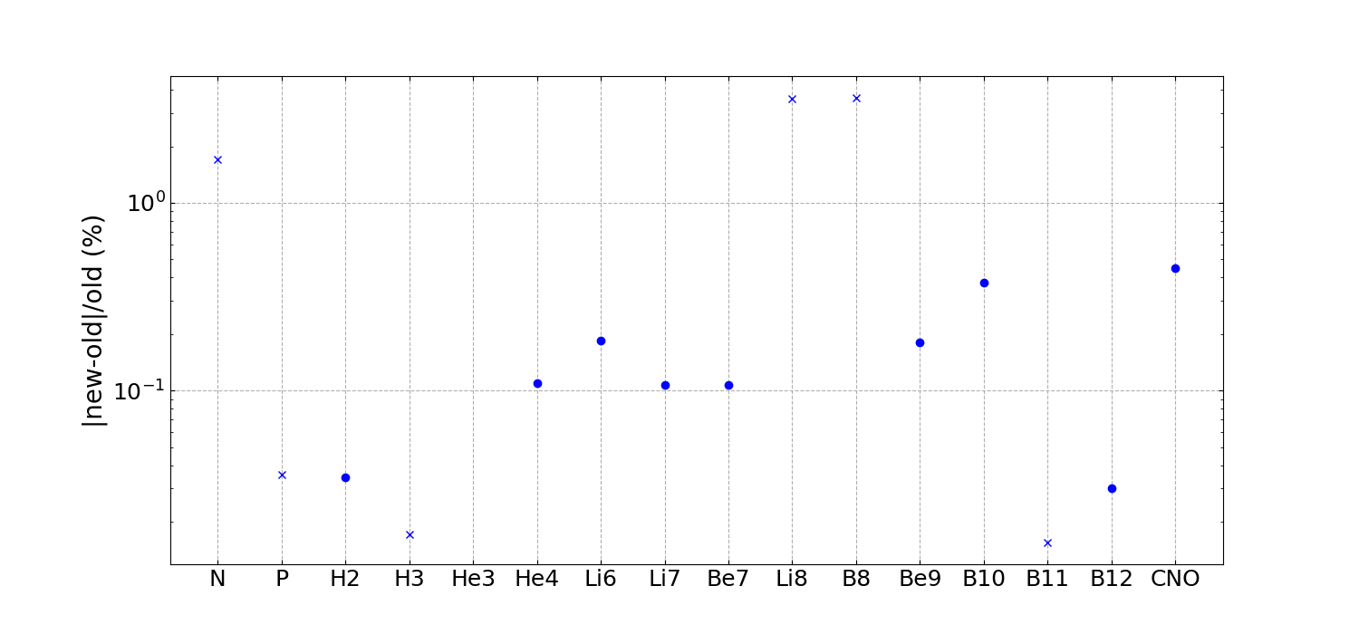
Figure 1: Absolute value of the relative difference between versions (in percentage) of the final primordial abundances for all nuclides computed in PArthENoPE. CNO includes all carbon, nitrogen and oxygen nuclides. Circles are positive relative differences and crosses correspond to negative differences. The difference for ³He/H is smaller than 0.001%.

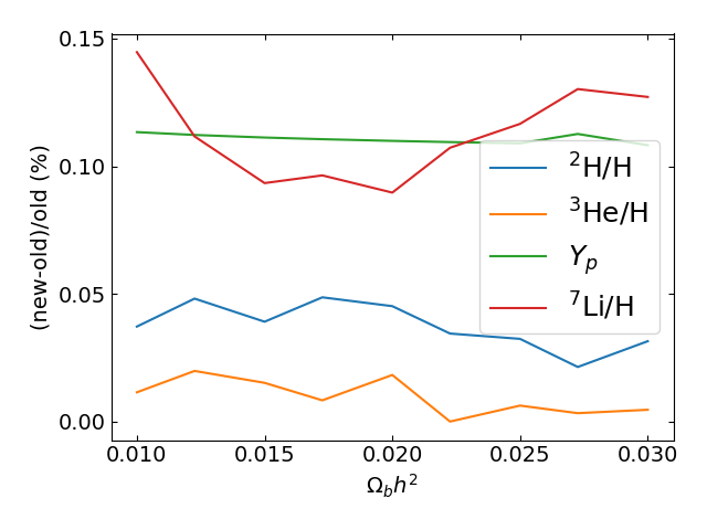
Figure 2: Relative difference between PArthENoPE 2.0 and PArthENoPE (in percentage) of the produced ${}^{2}{\rm H/H}$, ³He/H, $Y_{p}$ and ⁷Li/H for different values of the baryon density $\Omega_{b}h^{2}$.

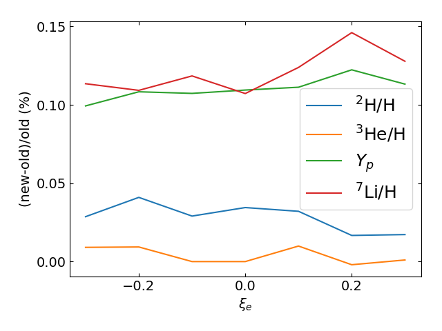
Figure 3: Same as Fig. 2 but varying the neutrino degeneracy parameter with $\xi_{e}=\xi_{\mu}=\xi_{\tau}$.

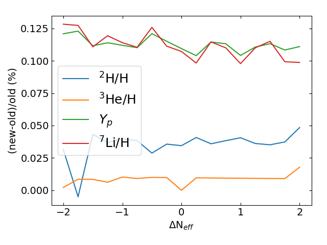
Figure 4: Same as Fig. 2 but varying the effective number of neutrinos ($\Delta N_{\rm eff}$).

IV Comparison with PArthENoPE

We have checked that the performance of PArthENoPE 2.0 is at least as good as that of PArthENoPE and we can recover a nice evolution of the different nuclides. For this purpose we compared the outputs of both versions using a benchmark model in which we choose the standard values $\Delta N_{\rm eff}=0$, $\eta_{10}=6.09389$ (corresponding to $\Omega_{b}h^{2}=0.02226$ Ade:2015xua ) and $\xi_{i}=0$.

In Fig. 1 we show the relative difference of the final abundances of all nuclides in percentage. The total abundance of carbon, nitrogen and oxygen nuclides is shown in a single column labelled CNO, i.e. the total metallicity produced during BBN, which is very small (of order $10^{-16}$) and largely dominated by ¹²C, see e.g. Iocco:2007km . As can be seen in the figure, the difference is below 1% for most of the nuclides; in particular, for deuterium and helium it is below $\sim 0.1$%.

In order to show the robustness of the new code beyond our benchmark model, we checked its behaviour in the parameter space when leaving free one of the three fixed parameters stated above. We show in Figures 2, 3 and 4 the relative difference between the output abundances of the four main nuclides from PArthENoPE and PArthENoPE 2.0 for different values of $\eta_{10}$ (for user convenience we report in the plot the values of $\Omega_{b}h^{2}$), $\xi_{e}=\xi_{\mu}=\xi_{\tau}$ and $\Delta N_{\rm eff}$, respectively. As can be seen in the plots, no relevant dependence on the value of the parameters is found, with the exception of ⁷Li as a function of the baryon density, but for some value of $\Omega_{b}h^{2}$ excluded by Planck results.

Note that the number of steps performed by the ODE system solver in PArthENoPE on each simulation is about 5 times that of PArthENoPE 2.0. However, as proved by the results shown in the above figures, this does not change the precision of the code and the difference in the number of steps is related with the internal construction of the different solvers.

V BBN analysis using PArthENoPE 2.0

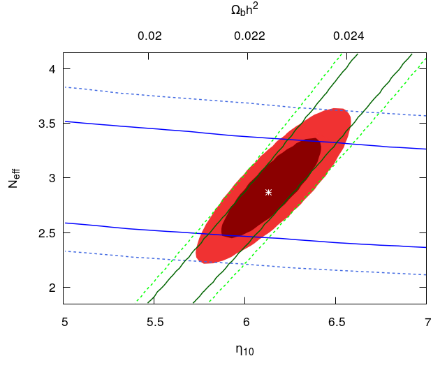
Figure 5: Allowed regions for the cosmological baryon density and the effective number of neutrinos from our BBN analysis, shown as contours at the $1\,\sigma$ and $2\,\sigma$ levels. For comparison, we also include the corresponding intervals for the experimental measurements of ⁴He (blue lines) and deuterium (green lines) alone.

In this section we illustrate the potentiality of the new version of PArthENo PE performing a BBN analysis, both in the standard case with a single free parameter ($\eta_{10}$) and in an extended scenario where the radiation content of the universe can vary via the parameter $N_{\rm eff}$. The theoretical output of the primordial abundances of the light nuclei from our code is compared with recent experimental data. Here we consider two recent measurements on the abundances of the main nuclides: deuterium Cooke:2017cwo and ${}^{4}\mathrm{He}$ Aver:2015iza (we treat all uncertainties to be $1\sigma$ throughout this section),

$${}^{2}\mathrm{H/H}=\left(2.527\pm 0.030\right)\cdot 10^{-5}$$ (23)

and

$$Y_{p}=0.2449\pm 0.0040~{}~{}~{}.$$ (24)

We used the abundances of both elements to constrain $\eta_{10}$ and $N_{\rm eff}$ defining a $\chi^{2}$-function as follows

$$\chi^{2}=\sum_{i}\frac{\left(X_{i}^{\rm th}\left(N_{\rm eff},\eta_{10}\right)-X_{i}^{\rm exp}\right)^{2}}{\sigma^{2}_{i,{\rm th}}+\sigma^{2}_{i,{\rm exp}}},$$ (25)

where $i=\{\,^{2}\mathrm{H/H}\,,\,Y_{p}\}$, $\sigma_{i,{\rm exp}}$ are the experimental errors as above and $\sigma_{i,{\rm th}}$ is the uncertainty due to propagation of nuclear process rates: $\sigma_{{}^{2}\mathrm{H/H},{\rm th}}=0.05\cdot 10^{-5}$ and $\sigma_{Y_{p},{\rm th}}=0.0003$ Coc:2015bhi .

When the effective number of neutrinos is fixed to its standard value, $N_{\rm eff}=3.045$, from our analysis we find that the baryon to photon number density is $\eta_{10}=6.23^{+0.12}_{-0.14}$. This corresponds to a present baryon density allowed by BBN of $\Omega_{b}h^{2}=0.0227\pm 0.0005$, in excellent agreement with the range $\Omega_{b}h^{2}=0.02218\pm 0.00015$ measured by Planck Aghanim:2016yuo . Instead, the ⁷Li abundance from PArthENoPE 2.0 for the best-fit value of $\eta_{10}$ is ${}^{7}{\rm Li/H}=4.69\cdot 10^{-10}$. This value clearly disagrees with the measurement ${}^{7}\mathrm{Li/H}=(1.58\pm 0.31)\cdot 10^{-10}$ Sbordone:2010zi , the already mentioned primordial lithium discrepancy.

The results of our BBN analysis when $N_{\rm eff}$ is left as a free parameter can be seen in Fig. 5. The allowed regions for $N_{\rm eff}$ and $\eta_{10}$ are shown at the 1 and $2\sigma$ levels, together with the bounds when only the experimental measurement of deuterium or ⁴He is considered. The corresponding allowed ranges are

$$N_{\rm eff}=2.87^{+0.24}_{-0.21}\qquad{\rm and}\qquad\eta_{10}=6.13\pm 0.13~{}(\Omega_{b}h^{2}=0.0224\pm 0.0005)$$ (26)

Both agree with the radiation content expected in the standard case ($N_{\rm eff}=3.045$) and the baryon density favoured by the analysis of data on CMB anisotropies by Planck Aghanim:2016yuo , respectively. Finally, we have included in our analysis the Planck measurement for $\Omega_{b}h^{2}$ as a gaussian prior. In this case, we obtain the allowed ranges $N_{\rm eff}=2.81^{+0.22}_{-0.21}$ and $\eta_{10}=6.082^{+0.022}_{-0.06}$ ($\Omega_{b}h^{2}=0.02224^{+0.00008}_{-0.00020}$).

VI Conclusions

CMB anisotropies, large-scale structures, gravitational lensing and BBN are an intertwined system of observables which test the cosmological evolution at different epochs. The quantity and quality of data coming from astrophysical measurements in the last decade, and those which will be available in the future, call for accurate tools providing theoretical predictions on cosmological observables to check the overall consistency of the picture of the evolution of the universe, as well as for investigating and constraining new physics beyond the present framework of fundamental interactions. In this perspective, in 2008 we developed the BBN numerical code PArthENoPE with two main goals: to create a tool with an increased level of accuracy of theoretical predictions on nuclide abundances (improved estimate of the neutron to proton weak conversion rates, detailed neutrino decoupling, reanalysis of nuclear network rates) which updated the works of Wagoner:1966pv ; Wagoner2 ; Wagoner:1972jh ; Kawano:1988vh ; Smith:1992yy , and to provide a public tool to researchers interested in the field which fulfills the requirements of precision and versatility. After almost ten years we have developed a new version of the code, PArthENoPE 2.0, whose new aspects and characteristics have been described in this paper. Apart from minor points, which will be detailed at the PArthENoPE web page, http://parthenope.na.infn.it, we have here outlined the main new features of PArthENoPE 2.0:

• We replaced the NAG libraries used for various purposes in the code, but which are not free software, with other libraries publicly available.

• PArthENoPE 2.0 is now interfaced with a Python file, which enhances the old main.f interface of the previous version and provides a more user friendly GUI for choosing interactively the initial parameters and running configuration.

We hope this new version of the code, which shares with PArthENoPE the same theoretical and numerical accuracy, but is more user friendly, will be useful to researchers interested in BBN-related studies.

Appendix A The PArthENoPE set of equations

Few typos and minor mistakes are contained in the Appendix A of the PArthENoPE reference paper parthenope . In this Appendix we summarize the PArthENoPE set of equations with the purpose of correcting these typos. We remind the reader that we use the dimensionless variables $z\equiv m_{e}/T$, $x=m_{e}\,a$, $\bar{z}=x/z=aT=T/T_{\nu}$. Moreover, as defined in parthenope ,

$${\mathcal{N}}(z)=\frac{1}{\bar{z}^{4}}\left(x\frac{d}{dx}\bar{\rho}_{\nu}\right)\Bigg{|}_{x=x(z)}\,\,\,, \bar{\rho}_{\nu}=a^{4}\,\rho_{\nu}=\left(\frac{x}{m_{e}}\right)^{4}\,\rho_{\nu}\,\,\,,$$ (27)

$$\rho=\rho_{e\gamma B}+\rho_{\nu}\,\,\,, {\rm p}={\rm p}_{e\gamma B}+{\rm p}_{\nu}~{}~{}~{},$$ (28)

$$\hat{\rho}=T^{-4}\,\rho=\left(\frac{z}{m_{e}}\right)^{4}\,\rho~{}~{}~{}, \hat{\rm p}=T^{-4}\,{\rm p}=\left(\frac{z}{m_{e}}\right)^{4}\,{\rm p}~{}~{}~{}.$$ (29)

Finally, in what follows we will also consider the energy density of electrons/positrons plus photons, $\rho_{e\gamma}$. The equation for the entropy conservation

$$\dot{\rho}=-\,3\,H~{}(\rho+{\rm p})~{}~{}~{},$$ (30)

once used the definitions (27)-(29) and expressing the total time derivative of $\hat{\rho}_{e\gamma B}$ via the partial derivatives with respect to $z$, ${\phi_{e}}$ and $X_{i}$, becomes

$$\left(\frac{\partial\hat{\rho}_{e\gamma B}}{\partial z}-\frac{4}{z}\,\hat{\rho}_{e\gamma B}+\frac{\partial\hat{\rho}_{e\gamma B}}{\partial{\phi_{e}}}\,\frac{d{\phi_{e}}}{dz}+\sum_{i}\frac{\partial\hat{\rho}_{e\gamma B}}{\partial{X_{i}}}\,\frac{dX_{i}}{dz}\right)\dot{z}=-\,3\,H\,(\hat{\rho}_{e\gamma B}+\hat{\rm p}_{e\gamma B})-H\,\mathcal{N}(z)~{}~{}~{}.$$ (31)

Proceeding in the same way, the equation for conservation of the total baryon number

$$\dot{n}_{B}=-\,3\,H\,n_{B}~{}~{}~{},$$ (32)

becomes

$$\left(\frac{\partial\hat{n}_{B}}{\partial z}+\frac{\partial\hat{n}_{B}}{\partial{\phi_{e}}}\frac{d{\phi_{e}}}{dz}+\sum_{i}\frac{\partial\hat{n}_{B}}{\partial{X_{i}}}\frac{dX_{i}}{dz}\right)\dot{z}=-\,3\,H\,\hat{n}_{B}~{}~{}~{}.$$ (33)

where we define $\hat{n}_{B}\equiv n_{B}/m_{e}^{3}=\hat{L}(z,{\phi_{e}})/(z^{3}\sum_{i}Z_{i}X_{i})$. Obtaining $\dot{z}$ from (33) and substituting into (31) we get

$$-\,3\,H\,\hat{n}_{B}\frac{\frac{\partial\hat{\rho}_{e\gamma B}}{\partial z}-\frac{4}{z}\hat{\rho}_{e\gamma B}+\frac{\partial\hat{\rho}_{e\gamma B}}{\partial{\phi_{e}}}\,\frac{d{\phi_{e}}}{dz}+\sum_{i}\frac{\partial\hat{\rho}_{e\gamma B}}{\partial{X_{i}}}\,\frac{dX_{i}}{dz}}{\frac{\partial\hat{n}_{B}}{\partial z}+\frac{\partial\hat{n}_{B}}{\partial{\phi_{e}}}\frac{d{\phi_{e}}}{dz}+\sum_{i}\frac{\partial\hat{n}_{B}}{\partial{X_{i}}}\frac{dX_{i}}{dz}}=-\,3\,H\,(\hat{\rho}_{e\gamma B}+\hat{\rm p}_{e\gamma B})-H\,\mathcal{N}(z)~{}~{}~{}.$$ (34)

By solving this equation with respect to $d{\phi_{e}}/dz$ (expressing $\hat{n}_{B}$ and its derivatives as function of $\hat{L}(z,{\phi_{e}})$) one gets the expression for $d{\phi_{e}}/dz$ used in PArthENoPE

$$\frac{d{\phi_{e}}}{dz}=\frac{1}{z}\frac{\hat{L}\,\kappa_{1}+\left(\hat{\rho}_{e\gamma}+\hat{\rm p}_{e\gamma B}+\frac{\mathcal{N}(z)}{3}\right)\,\kappa_{2}}{\hat{L}\,\frac{\partial\hat{\rho}_{e}}{\partial{\phi_{e}}}-\frac{\partial\hat{L}}{\partial{\phi_{e}}}\left(\hat{\rho}_{e\gamma}+\hat{\rm p}_{e\gamma B}+\frac{\mathcal{N}(z)}{3}\right)}~{}~{}~{},$$ (35)

where

$$\kappa_{1} = 4\,\left(\hat{\rho}_{e}+\hat{\rho}_{\gamma}\right)+\frac{3}{2}~{}\hat{\rm p}_{B}-z\,\frac{\partial\hat{\rho}_{e}}{\partial z}-z\,\frac{\partial\hat{\rho}_{\gamma}}{\partial z}-\frac{z^{2}\,\hat{L}}{\sum_{j}Z_{j}\,X_{j}}\sum_{i}\left(\Delta\widehat{M}_{i}+\frac{3}{2\,z}\right)\widetilde{\Gamma}_{i}~{}~{}~{},$$

$$\kappa_{2} = z\,\frac{\partial\hat{L}}{\partial z}-3\,\hat{L}-z\,\hat{L}\,\frac{\displaystyle\sum_{i}~{}Z_{i}\,\widetilde{\Gamma}_{i}}{\displaystyle\sum_{j}~{}Z_{j}\,X_{j}}~{}~{}~{}.$$ (37)

In the previous equations, $\Delta\widehat{M}_{i}$ stands for the i-th nuclide mass excess normalized to $m_{e}$, whereas $\widetilde{\Gamma}_{i}\equiv d\Gamma_{i}/dz$.

We now need $\dot{z}$ in order to calculate $\widetilde{\Gamma}_{i}=\Gamma_{i}/\dot{z}$. At this aim, one can substitute Eq. (35) in (33), getting after some rearrangements

$$\dot{z}=-3\,z\,H\,\frac{\hat{L}\,\frac{\partial\hat{\rho}_{e}}{\partial{\phi_{e}}}-\frac{\partial\hat{L}}{\partial{\phi_{e}}}\left(\hat{\rho}_{e\gamma}+\hat{\rm p}_{e\gamma B}+\frac{\mathcal{N}(z)}{3}\right)}{\kappa_{1}\,\frac{\partial\hat{L}}{\partial{\phi_{e}}}+\kappa_{2}\,\frac{\partial\hat{\rho}_{e}}{\partial{\phi_{e}}}}~{}~{}~{}.$$ (38)

The equations for the abundances (5) then assume the form used in PArthENoPE,

$$\frac{dX_{i}}{dz}=-\frac{\widehat{\Gamma}_{i}}{3\,z\,\widehat{H}}\,\frac{\kappa_{1}\,\frac{\partial\hat{L}}{\partial{\phi_{e}}}+\kappa_{2}\,\frac{\partial\hat{\rho}_{e}}{\partial{\phi_{e}}}}{\hat{L}\,\frac{\partial\hat{\rho}_{e}}{\partial{\phi_{e}}}-\frac{\partial\hat{L}}{\partial{\phi_{e}}}\left(\hat{\rho}_{e\gamma}+\hat{\rm p}_{e\gamma B}+\frac{\mathcal{N}(z)}{3}\right)}~{}~{}~{}.$$ (39)

References

- (1) G. Hinshaw et al. [WMAP Collaboration], Astrophys. J. Suppl. 208 (2013) 19
- (2) P.A.R. Ade et al. [Planck Collaboration], Astron. Astrophys. 594 (2016) A13
- (3) L. Sbordone et al., Astron. Astrophys. 522 (2010) A26
- (4) F. Iocco, G. Mangano, G. Miele, O. Pisanti and P.D. Serpico, Phys. Rept. 472 (2009) 1
- (5) K.N. Abazajian et al., preprint arXiv:1204.5379 [hep-ph]
- (6) R.E. Lopez and M.S. Turner, Phys. Rev. D 59 (1999) 103502
- (7) S. Esposito, G. Mangano, G. Miele and O. Pisanti, Nucl. Phys. B 540 (1999) 3
- (8) S. Esposito, G. Mangano, G. Miele and O. Pisanti, Nucl. Phys. B 568 (2000) 421
- (9) S. Esposito, G. Mangano, G. Miele and O. Pisanti, JHEP 09 (2000) 038
- (10) P.D. Serpico et al., JCAP 12 (2004) 010
- (11) S. Hannestad and J. Madsen, Phys. Rev. D 52 (1995) 1764
- (12) A.D. Dolgov, S.H. Hansen and D.V. Semikoz, Nucl. Phys. B 503 (1997) 426
- (13) G. Mangano, G. Miele, S. Pastor and M. Peloso, Phys. Lett. B 534 (2002) 8
- (14) G. Mangano et al., Nucl. Phys. B 729 (2005) 221
- (15) J. Birrell, C.T. Yang and J. Rafelski, Nucl. Phys. B 890 (2014) 481
- (16) P.F. de Salas and S. Pastor, JCAP 07 (2016) 051
- (17) E. Grohs and G.M . Fuller, Nucl. Phys. B 923 (2017) 222
- (18) C. Patrignani et al. (Particle Data Group), Chin. Phys. C 40 (2016) 100001
- (19) R.H. Cyburt, Phys. Rev. D 70 (2004) 023505
- (20) C. Angulo et al., Nucl. Phys. A 656 (1999) 3. See also the URL: http://pntpm.ulb.ac.be/Nacre/nacre.htm
- (21) Y. Xu, et al., Nucl. Phys. A 918 (2013) 61
- (22) O. Pisanti et al., Comput. Phys. Commun. 178 (2008) 956. See also the URL: http://parthenope.na.infn.it/
- (23) R.V. Wagoner, W.A. Fowler and F. Hoyle, Astrophys. J. 148 (1967) 3
- (24) R.V. Wagoner, Astrophys. J. Suppl. 18 (1969) 247
- (25) R.V. Wagoner, Astrophys. J. 179 (1973) 343
- (26) L. Kawano, preprint FERMILAB-PUB-88-034-A
- (27) M.S. Smith, L.H. Kawano and R.A. Malaney, Astrophys. J. Suppl. 85 (1993) 219
- (28) D.S. Leonard, H.J. Karwowski, C.R. Brune, B.M. Fisher and E.J. Ludwig, Phys. Rev. C 73 (2006) 045801
- (29) See the URL: http://parthenope.na.infn.it/docs/changelog.txt
- (30) E.G. Adelberger et al., Rev. Mod. Phys. 83 (2011) 195
- (31) G. Mangano, G. Miele, S. Pastor, O. Pisanti and S. Sarikas, Phys. Lett. B 708 (2012) 1
- (32) E. Castorina et al., Phys. Rev. D 86 (2012) 023517
- (33) F. Capozzi et al., Phys. Rev. D 95 (2017) 096014
- (34) I. Esteban, M.C. González-García, M. Maltoni, I. Martínez-Soler and T. Schwetz, JHEP 01 (2017) 087
- (35) P.F. de Salas, D.V. Forero, C.A. Ternes, M. Tórtola and J.W.F. Valle, preprint arXiv:1708.01186 [hep-ph]
- (36) W.H. Press, S.A. Teukolsky, W.T. Vetterling and B.P. Flannery, Numerical Recipes in Fortran 77, Ed. Cambridge University Press
- (37) See the URL: http://computation.llnl.gov/casc/odepack/
- (38) F. Iocco, G. Mangano, G. Miele, O. Pisanti and P.D. Serpico, Phys. Rev. D 75 (2007) 087304
- (39) R. Cooke, M. Pettini and C.C. Steidel, preprint arXiv:1710.11129 [astro-ph.CO]
- (40) E. Aver, K.A. Olive and E.D. Skillman, JCAP 07 (2015) 011
- (41) A. Coc et al., Phys. Rev. D 92 (2015) 123526
- (42) N. Aghanim et al. [Planck Collaboration], Astron. Astrophys. 596 (2016) A107