Path-integral simulation of graphene monolayers under tensile stress

Abstract

Finite-temperature properties of graphene monolayers under tensile stress have been studied by path-integral molecular dynamics (PIMD) simulations. This method allows one to consider the quantization of vibrational modes in these crystalline membranes and to analyze the influence of anharmonic effects in the membrane properties. Quantum nuclear effects turn out to be appreciable in structural and thermodynamic properties of graphene at low temperature, and they can even be noticeable at room temperature. Such quantum effects become more relevant as the applied stress is increased, mainly for properties related to out-of-plane atomic vibrations. The relevance of quantum dynamics in the out-of-plane motion depends on the system size, and is enhanced by tensile stress. For applied tensile stresses, we analyze the contribution of the elastic energy to the internal energy of graphene. Results of PIMD simulations are compared with calculations based on a harmonic approximation for the vibrational modes of the graphene lattice. This approximation describes rather well the structural properties of graphene, provided that the frequencies of ZA (flexural) acoustic modes in the transverse direction include a pressure-dependent correction.

I Introduction

In recent years there has been a surge of interest on two-dimensional materials, and graphene in particular, due to their unusual electronic, elastic and thermal properties.Geim and Novoselov (2007); Castro Neto et al. (2009); Flynn (2011); Roldan et al. (2017) In fact, graphene displays high values of thermal conductivity,Ghosh et al. (2008); Nika et al. (2009); Balandin (2011) as well as large in-plane elastic constants.Lee et al. (2008) Its mechanical properties are also important for possible applications, such as cooling of electronic devices.Seol et al. (2010); Prasher (2010)

The structural arrangement for pure defect-free graphene corresponds to a planar honeycomb lattice. At finite temperatures, there appear out-of-plane displacements of the C atoms, and for $T\to 0$, quantum fluctuations related to zero-point motion give rise to a departure of strict planarity of the graphene sheet.Herrero and Ramírez (2016) In particular, one has low-lying vibrational excitations associated to large-scale ripples perpendicular to the plane.Fasolino et al. (2007) Moreover, a graphene sheet can actually bend and depart from planarity for other reasons, such as the presence of defects and external stresses.Meyer et al. (2007); de Andres et al. (2012a)

A thin membrane crumples in the presence of a compressive stress. This behavior has been investigated during the last three decades in lipid membranesEvans and Rawicz (1990); Safran (1994) and polymer films.Cerda and Mahadevan (2003); Wong and Pellegrino (2006) In graphene, crumpling originates from out-of-plane phonons as well as from static wrinkling, and has been observed in both supported and freestanding samples.Kirilenko et al. (2011); Nicholl et al. (2015) Mechanical properties such as stiffness and bending rigidity can be renormalized due to crumpling.Ruiz-Vargas et al. (2011); Kosmrlj and Nelson (2013, 2014) For graphene, it has been found that the maximum compressive stress that a freestanding sheet can sustain without crumpling decreases with system size, and has been estimated to be about 0.1 N/m at room temperature in the thermodynamic limit.Ramírez and Herrero (2017)

A tensile stress applied in the graphene plane does not affect the planarity of the sheet, but causes appreciable changes in the elastic properties of the material.López-Polín et al. (2017) Thus, it has been observed that the in-plane Young modulus is increased by a factor of three when applying a stress of 1 N/m.Ramírez and Herrero (2017) The bending rigidity $\kappa$ does also change with the tensile stress, and in fact it decreases but not so critically as the in-plane elastic constants. In this context, it is important to note that the actual area per atom, $A$, is not readily measurable, and the accessible observable is usually its projection, $A_{p}$, onto the mean plane of the membrane ($A_{p}\leq A$). Thus, one may refer the elastic properties of graphene either to the area $A$ or to $A_{p}$, which may behave in very different ways. For example, a negative thermal expansion coefficient is found for graphene when one refers to $A_{p}$, but the thermal expansion associated to the area $A$ is positive.Pozzo et al. (2011); Herrero and Ramírez (2016)

Recent experimental and theoretical work has shown the influence of strain in several characteristics of graphene, such as electronic transport, optical properties, and the formation of moiré patterns.Woods et al. (2014) Similar properties have been also studied in other two-dimensional materials, as metallic dichalcogenides.Amorim et al. (2016)

Equilibrium and dynamical properties of graphene have been studied earlier by using Monte Carlo and molecular dynamics simulations. These simulations were based on ab-initio,Shimojo et al. (2008); Pozzo et al. (2011); de Andres et al. (2012b); Chechin et al. (2014) tight-binding,Herrero and Ramírez (2009); Cadelano et al. (2009); Akatyeva and Dumitrica (2012); Lee et al. (2013) and empirical interatomic potentials.Fasolino et al. (2007); Shen et al. (2013); Los et al. (2009); Ramírez et al. (2016); Magnin et al. (2014); Los et al. (2016) In most of these simulations, C atoms were treated as classical particles, which is accurate at relatively high temperatures but is not suitable to study thermodynamic variables at low temperature. The quantum character of the atomic motion can be taken into account by employing path-integral simulations, which allow to consider quantum and thermal fluctuations in many-body systems at finite temperatures.Gillan (1988); Ceperley (1995) Path-integral simulations of a single graphene sheet have been lately performed to study equilibrium properties of this material.Brito et al. (2015); Herrero and Ramírez (2016) Moreover, nuclear quantum effects have been studied by a combination of density-functional theory and a quasi-harmonic approximation for vibrational modes in this crystalline membrane.Mounet and Marzari (2005); Shao et al. (2012)

In this paper, we employ path-integral molecular dynamics (PIMD) simulations to study structural and vibrational properties of graphene under tensile stress. We consider different sizes for the simulation cell, as finite-size effects are known to be important for some properties of graphene.Gao and Huang (2014); Los et al. (2016); Herrero and Ramírez (2016) The magnitude of nuclear quantum effects in the graphene properties is assessed by comparing the results of PIMD simulations with data obtained from classical simulations. We find that quantum effects are relevant to describe the temperature and pressure dependence of graphene’s real and in-plane areas, as well as to describe the amplitude of the out-of-plane motion, especially at low temperatures. Our data indicate that the relevance of nuclear quantum effects increases as tensile stress is raised. Results of PIMD simulations are compared with data derived from a harmonic approximation for the out-of-plane vibrations. This approximation turns out to be rather accurate, provided that the vibrational frequencies of ZA acoustic modes are conveniently renormalized for different applied stresses.

The paper is organized as follows. In Sec. II, we present the computational method used in the simulations. Structural properties such as in-plane $A_{p}$ and real area $A$ are given in Sec. III as a function of applied stress. Results for the internal, vibrational, and elastic energy of graphene are discussed in Sec. IV. In Sec. V we study the out-of-plane atomic motion, with emphasis on the competition between classical-like and quantum dynamics. In Sec. VI we summarize the main results.

II Computational Method

We use the PIMD method to obtain equilibrium properties of graphene under tensile stress. This procedure is based on the Feynman path-integral formulation of statistical mechanics, a nonperturbative technique to study many-body quantum systems at finite temperatures.Feynman (1972) The implementation of this formulation for numerical simulations is based on an isomorphism between the quantum system and a fictitious classical system, in which each quantum particle is described by a ring polymer (corresponding to a cyclic quantum path) composed of $N_{\rm Tr}$ (Trotter number) beads.Kleinert (1990) This becomes exact in the limit $N_{\rm Tr}\to\infty$. Details on this simulation technique can be found elsewhere.Chandler and Wolynes (1981); Gillan (1988); Ceperley (1995); Herrero and Ramírez (2014) The dynamics in PIMD is artificial, since it does not correspond to the actual dynamics of the real quantum particles. However, it is useful for sampling the many-body configuration space, yielding accurate results for time-independent equilibrium properties of the actual quantum system.

The Born-Oppenheimer surface for the nuclear dynamics is derived here from an effective empirical potential, developed for carbon-based systems, namely the so-called LCBOPII.Los et al. (2005) This is a long-range carbon bond order potential, which was previously used to perform classical simulations of diamond,Los et al. (2005) graphite,Los et al. (2005) liquid carbon,Ghiringhelli et al. (2005a) as well as graphene sheets.Zakharchenko et al. (2009); Fasolino et al. (2007); Los et al. (2016) A relevant application of this effective potential was the calculation of the carbon phase diagram including diamond, graphite, and the liquid, and showing its precision by comparison of the predicted diamond-graphite line with experimental results.Ghiringhelli et al. (2005b)

The LCBOPII potential has been more recently employed to study graphene, giving a good description of elastic properties such as the Young’s modulus.Zakharchenko et al. (2009); Politano et al. (2012) According to previous simulations,Ramírez et al. (2016); Herrero and Ramírez (2016); Ramírez and Herrero (2017) the original LCBOPII parameterization has been slightly modified to increase the zero-temperature bending constant of graphene from 1.1 eV to a value of 1.49 eV, more consistent with experimental data.Lambin (2014) This effective potential was lately used to perform PIMD simulations, allowing to assess the extent of quantum effects in graphene sheets from a comparison with results of classical simulations.Herrero and Ramírez (2016)

Other effective interatomic potentials have been employed in recent years to study various properties of graphene. In particular, the AIREBO potential model has been widely used in this field.Sfyris et al. (2015); Memarian et al. (2015); Zou et al. (2016); Anastasi et al. (2016); Ghasemi and Rajabpour (2017) Comparing the LCBOPII and AIREBO models, we find that they yield very similar equilibrium C–C distance and in-plane thermal expansion coefficient, as derived from classical molecular dynamics simulations.Memarian et al. (2015); Ghasemi and Rajabpour (2017); Herrero and Ramírez (2016) Results for the Young’s modulus of graphene derived from the LCBOPII potential are closer to those given by ab initio calculations.Memarian et al. (2015)

The calculations presented here were carried out in the isothermal-isobaric ensemble, where we fix the number of carbon atoms ($N$), the applied stress ($P$), and the temperature ($T$). We employed effective algorithms for carrying out PIMD simulations in this statistical ensemble, as those presented in the literature.Tuckerman et al. (1992); Tuckerman and Hughes (1998); Martyna et al. (1999); Tuckerman (2002) Specifically, we used staging variables to define the bead coordinates, and the constant-temperature ensemble was achieved by coupling chains of four Nosé-Hoover thermostats. A supplementary chain of four barostats was coupled to the area of the simulation box to give the required pressure $P$.Tuckerman and Hughes (1998); Herrero and Ramírez (2014) The kinetic energy $K$ has been calculated by using the so-called virial estimator, which has a statistical uncertainty smaller than the potential energy, $V$, of the system.Herman et al. (1982); Tuckerman and Hughes (1998) Other technical details about the simulations presented here are the same as those given elsewhere.Herrero et al. (2006); Herrero and Ramírez (2011); Ramírez et al. (2012)

Atomic forces were analytically derived from position derivatives of the instantaneous potential energy $U$ (note that $V=\langle U\rangle$). The estimator of the two-dimensional (2D) stress tensor ${\bf\tau}$ is the same as that employed in previous works,(Ramírez et al., 2016; Ramírez and Herrero, 2017) and its formulation for PIMD simulations of graphene is similar to that given earlier for three-dimensional (3D) solids.Ramírez et al. (2008); Herrero and Ramírez (2014) Details on the pressure estimator employed here are presented in Appendix A. The mechanical stress $P$ in the $(x,y)$ plane of graphene is obtained from the trace of the tensor ${\bf\tau}$:

$$P=\frac{1}{2}\left(\tau_{xx}+\tau_{yy}\right)\,.$$ (1)

Note that in the case of applying a large compressive stress ($P>0$, not considered here), one may have severe bending or crumpling of the graphene sheet. In this case the in-plane stress $P$ may appreciably differ from the actual stress felt by the real graphene surface (related to the area $A$).Ramírez and Herrero (2017); Fournier and Barbetta (2008)

We consider rectangular simulation cells with similar side lengths $L_{x}$ and $L_{y}$ in the $x$ and $y$ directions of the reference plane, and periodic boundary conditions were assumed. Sampling of the configuration space has been carried out at temperatures between 12 K and 2000 K. For comparison with results of PIMD simulations, some classical molecular dynamics (MD) simulations have been also performed. In our context this is achieved by by setting $N_{\rm Tr}$ = 1. For the quantum simulations, $N_{\rm Tr}$ was taken proportional to the inverse temperature: $N_{\rm Tr}\,T$ = 6000 K, which roughly gives a constant precision in the PIMD results at different temperatures.Herrero et al. (2006); Herrero and Ramírez (2011); Ramírez et al. (2012) Cells of size up to 8400 and 14720 atoms were considered for PIMD and classical MD simulations, respectively. For a given temperature, a typical simulation run consisted of $3\times 10^{5}$ PIMD steps for system equilibration, followed by $4\times 10^{6}$ steps for the calculation of ensemble average properties.

III Structural properties

The simulations presented here were performed in the isothermal-isobaric ensemble, as explained above in Sec. II. Thus, in a simulation run we fix the number of carbon atoms $N$, the temperature $T$, and the applied stress $P$ in the $(x,y)$ plane, allowing for changes in the in-plane area of the simulation cell for which periodic boundary conditions are assumed. Carbon atoms are free to move in the out-of-plane direction ($z$ coordinate), and in general any measure of the real surface of a graphene sheet at $T>0$ should give a value larger than the area of the simulation cell in the $(x,y)$ plane. In this line, there has appeared in recent years a discussion in the context of biological membranes, dealing with the question whether it is more convenient to describe the properties of those membranes using the concept of a real surface rather than a projected (in-plane) surface.Imparato (2006); Waheed and Edholm (2009); Chacón et al. (2015) The same question has been also recently raised for crystalline membranes such as graphene.Pozzo et al. (2011); Herrero and Ramírez (2016); Nicholl et al. (2017); Ramírez and Herrero (2017) This can be important for addressing the calculation of thermodynamic properties, because the in-plane area $A_{p}$ is the variable conjugate to the stress $P$ used in our simulations, and the real area $A$ (also called effective, true, or actual area in the literatureImparato (2006); Fournier and Barbetta (2008); Waheed and Edholm (2009); Chacón et al. (2015)) is conjugate to the usually-called surface tension.Safran (1994) The difference $A-A_{p}$ has been recently denoted as hidden area by Nicholl et al.Nicholl et al. (2017)

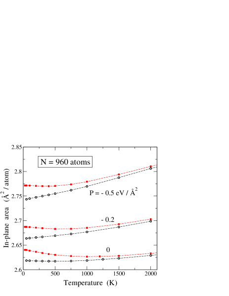
Figure 1: In-plane area $A_{p}$ vs. temperature for graphene, as derived from classical (open circles) and PIMD simulations (solid squares) for $N$ = 960 and different stresses. From bottom to top: $P$ = 0, $-0.2$, and $-0.5$ eV Å^-2. Error bars are less than the symbol size. Lines are guides to the eye.

The real area $A$ in 3D space is calculated here by a triangulation based on the atomic positions along a simulation run. $A$ is obtained from the areas associated to $N/2$ structural hexagons. Each hexagon contributes by a sum of six triangles, each one formed by the positions of two neighboring carbon atoms and the barycenter of the hexagon (mean point of its six vertices).Ramírez and Herrero (2017) There are other similar definitions that can be employed for the area $A$, as those based on the interatomic distance C–C.Hahn et al. (2016); Herrero and Ramírez (2016) The area $A$ based on triangulation employed here seems more precise to deal with the 2D nature of a graphene layer in 3D space. It has been shown earlier that $A$ has a very small size effect, in fact negligible in comparison with that appearing for $A_{p}$.Ramírez and Herrero (2017)

In Fig. 1 we show the temperature dependence of the in-plane area $A_{p}$, obtained from classical MD (open circles) and PIMD simulations (solid squares) for a supercell with $N$ = 960 atoms. Results are given for $P$ = 0, $-0.2$, and $-0.5$ eV Å^-2. Tensile stress causes not only an increase in $A_{p}$, but its temperature dependence also changes. For each considered value of the stress, the curve $A_{p}(T)$ derived from quantum simulations displays a minimum, that shifts to lower temperatures as the tensile stress is increased. Thus, such a minimum evolves from $T_{m}\approx$ 1000 K for $P=0$ to $\approx$ 400 K for $P=-0.5$ eV Å^-2. In the classical simulations, however, one finds a shallow minimum for $P=0$, that is absent for the tensile stresses shown in Fig. 1 (in fact we did not observe it for $P=-0.1$ eV Å^-2 either, not shown in the figure). The classical results for $P=0$ are similar to those found in earlier classical Monte Carlo and MD simulations of graphene single layers.Zakharchenko et al. (2009); Gao and Huang (2014); Brito et al. (2015)

At low $T$ the results of PIMD simulations verify $dA_{p}/dT\to 0$, i.e., the corresponding curves shown in Fig. 1 (solid symbols) become flat close to $T=0$, as required by the third law of thermodynamics. In the limit $T\to 0$, the difference between quantum and classical results converges to 0.022 Ų/atom in the absence of applied stress ($P=0$). This difference decreases for rising temperature, as nuclear quantum effects become less important. For $P=-0.5$ eV Å^-2, we find for $T\to 0$ a difference of 0.031 Ų/atom. The increase in $A_{p}$ at low temperature is due to zero-point motion associated to in-plane acoustic modes (LA and TA). The frequency of these modes decreases for increasing $A_{p}$ (i.e., when tensile stress is increased, according to positive Grüneisen parameters), and therefore their vibrational amplitudes are larger. This causes a larger zero-point expansion of $A_{p}$ for larger tensile stress.

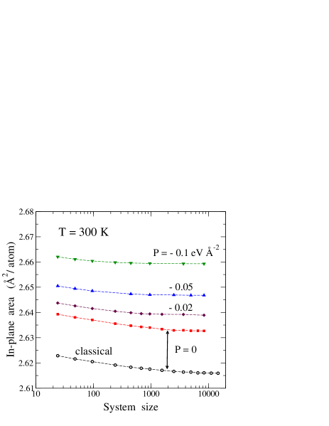
Figure 2: In-plane area $A_{p}$ vs. system size, as derived from PIMD simulations for $T$ = 300 K and various tensile stresses (solid symbols). From top to bottom: $P$ = $-0.1$ (triangles down), $-0.05$ (triangles up), $-0.02$ (diamonds), and 0 eV Å^-2 (squares). For comparison, open squares indicate results of classical MD simulations for $P$ = 0. Error bars are less than the symbol size. Lines are guides to the eye.

The presence of a minimum in the $A_{p}(T)$ curves derived from PIMD simulations is due to two competing effects, as discussed earlier for graphene without stress.Gao and Huang (2014); Michel et al. (2015); Herrero and Ramírez (2016) On one hand, the area $A$ increases as temperature is raised, and on the other hand, surface bending gives rise to a decrease in its 2D projection, i.e., $A_{p}$. At low $T$, this decrease associated to out-of-plane motion dominates the thermal expansion of the real surface, and $dA_{p}/dT<0$. For the quantum results, the thermal expansion at low $T$ is very small compared to the classical calculations for which $\lim_{T\to 0}dA/dT>0$, thus causing a more appreciable decrease in $A_{p}$ for raising $T$ in the quantum case. At high temperatures, the increase in $A$ predominates over the contraction in the projected area due to out-of-plane motion.

For unstressed graphene it has been indicated that finite-size effects can be important for several structural properties of the crystalline membrane.Herrero and Ramírez (2016); Ramírez and Herrero (2017) It is now worthwhile to consider finite-size effects for the in-plane area of graphene under stress. In Fig. 2 we present the size dependence of $A_{p}$ for several tensile stresses. In all cases, $A_{p}$ decreases for increasing $N$, and reaches a well-defined plateau for large sizes. One observes that the convergence to the large-size value is faster for larger tensile stress. Moreover, the difference between the large-size limit and the value corresponding to $N$ = 24 (the smallest supercell considered here) appreciably decreases from $6.7\times 10^{-3}$ Ų/atom for $P=0$ to $2.8\times 10^{-3}$ Ų/atom for $P=-0.1$ eV Å^-2.

For comparison, we also present in Fig. 2 results for $A_{p}(N)$ derived from classical MD simulations at 300 K. The difference between quantum and classical results for $P$ = 0 amounts to 0.017 Ų/atom, and it is nearly constant for the system sizes considered here. This difference increases to 0.022 Ų/atom at $P=0$ in the low-temperature limit, as indicated above (see Fig. 1). For $P=-0.1$ eV Å^-2 and $T=300$ K, our classical simulations yield an $A_{p}(N)$ curve similar to the quantum one (not shown in Fig. 2 to avoid overcrowding). In particular, for a system size $N=960$, we found an in-plane area $A_{p}$ = 2.6423 Ų/atom, so that the difference between classical and quantum results at this tensile stress is similar to that found for $P=0$. It is interesting to note that the increase in area $A_{p}$ due to quantum nuclear motion at 300 K is the same as that caused by a relatively large tensile stress of about $-0.07$ eV Å^-2 ($\sim-1$ N/m).

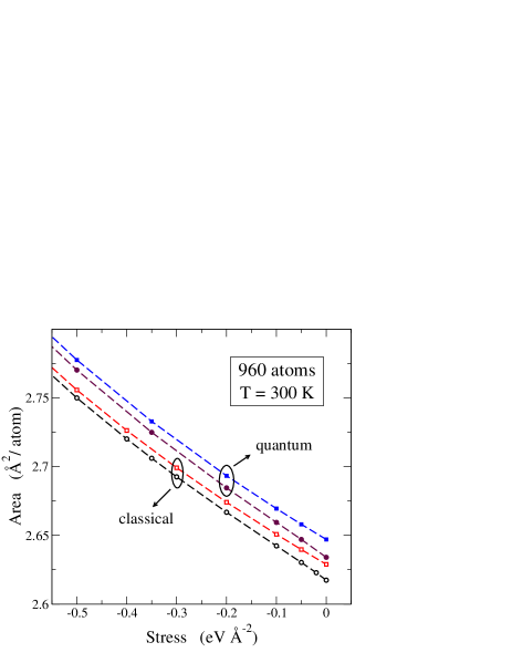
Figure 3: Real area $A$ and in-plane area $A_{p}$ of graphene vs. tensile stress, as derived from classical (open symbols) and PIMD simulations (solid symbols) for $N$ = 960 and $T$ = 300 K. Squares and circles correspond to $A$ and $A_{p}$, respectively. Error bars are less than the symbol size. Lines are guides to the eye.

We now turn to the real surface of graphene and its measure through the area $A$. It was shown earlier from simulations at $P=0$ that the surface $A$ is larger than $A_{p}$, and the difference between both increases with temperature. This is clear from the fact that $A_{p}$ is a 2D projection of $A$, and the actual surface becomes increasingly bent as temperature is raised and the amplitude of out-of-plane atomic vibrations becomes larger. An important difference between the temperature dependence of $A$ and $A_{p}$ is that the latter first decreases for increasing $T$ and then it increases at higher $T$, with a minimum at a temperature $T_{m}$. For rising tensile stress, the vibrational amplitude in the $z$ direction decreases (see below), so that the temperature $T_{m}$ of minimum $A_{p}$ is lowered. This becomes even clearer in the results of classical simulations, for which the shallow minimum in the curve $A_{p}(T)$ disappears at relatively low pressures, and it is not observed in the data presented for $P$ = $-0.2$ and $-0.5$ eV Å^-2 in Fig. 1. For the area $A$ one does not observe the decrease displayed by $A_{p}$ in both classical and quantum simulations at low temperatures (see Ref. Herrero and Ramírez, 2016 for results at $P=0$).

In Fig. 3 we present the areas $A$ and $A_{p}$ vs. tensile stress for a simulation cell including 960 atoms. In both cases, we present results from classical (open symbols) and PIMD (solid symbols) simulations. Circles correspond to the in-plane area $A_{p}$, whereas squares represent data for the real area $A$. One notices that quantum effects are appreciable at room temperature. The main aspects of this figure are the following. Tensile stress causes an increase of about 5% in both $A$ and $A_{p}$ from $P=0$ to $-0.5$ eV Å^-2. Moreover, quantum nuclear effects cause in both cases a surface expansion of about 0.02 Ų/atom, which increases slightly as the tensile stress is raised.

To make connection of our results derived from atomistic simulations with an analytical formulation of crystalline membranes, we note that the relation between $A$ and $A_{p}$ can be expressed in the continuum limit (macroscopic view) asImparato (2006); Waheed and Edholm (2009); Ramírez and Herrero (2017)

$$A=\int_{A_{p}}dx\,dy\,\sqrt{1+(\nabla h(x,y))^{2}}\;,$$ (2)

where $h(x,y)$ is the height of the membrane surface, i.e. the distance to the reference $(x,y)$ plane. The difference $A-A_{p}$ can be calculated in a classical approach by Fourier transformation of the r.h.s. of Eq. (2).Safran (1994); Chacón et al. (2015); Ramírez and Herrero (2017) This requires the introduction of a dispersion relation $\omega({\bf k})$ for out-of-plane modes (ZA band), where ${\bf k}=(k_{x},k_{y})$ are 2D wavevectors. The frequency dispersion in this acoustic (flexural) band can be well approximated by the expression $\rho\,\omega^{2}=\sigma k^{2}+\kappa k^{4}$, consistent with an atomic description of grapheneRamírez et al. (2016) ($k=|{\bf k}|$; $\rho$, surface mass density; $\sigma$, effective stress; $\kappa$, bending modulus). The effective stress $\sigma$ can be written as $\sigma=\sigma_{0}-P$, with a term $\sigma_{0}$ that appears at finite temperature even in the absence of an applied stress ($P=0$) due to out-of-plane motion (at 300 K, $\sigma_{0}\approx 6\times 10^{-3}$ eV Å^-2).Ramírez et al. (2016)

After Fourier transformation one has for the area per atom:Safran (1994); Chacón et al. (2015)

$$A=A_{p}+\frac{k_{B}T}{2N}\sum_{\bf k}\frac{1}{\sigma+\kappa k^{2}}\,.$$ (3)

For large $N$ the sum in Eq. (3) can be approximated by an integral:Ramírez and Herrero (2017)

$$A=A_{p}\left(1+\frac{k_{B}T}{4\pi}\int_{k_{0}}^{k_{m}}dk\frac{k}{\sigma+\kappa k^{2}}\right)\,.$$ (4)

The limits in the integral are the cut-off $k_{m}=(2\pi/A_{p})^{1/2}$ and the size-dependent minimum wavevector $k_{0}=2\pi/L$, with $L=(NA_{p})^{1/2}$. The integral in Eq. (4) converges provided that $\sigma>0$, which is the case here. It allows us to explicitly write the size-dependent ratio $A/A_{p}$ as

$$\frac{A}{A_{p}}=\left(\frac{A}{A_{p}}\right)_{\infty}-\frac{k_{B}T}{8\pi\kappa}\ln\left(1+\frac{4\pi^{2}\kappa}{NA_{p}\sigma}\right)$$ (5)

with the large-size limit ($N\to\infty$ or $k_{0}\to 0$):

$$\left(\frac{A}{A_{p}}\right)_{\infty}=1+\frac{k_{B}T}{8\pi\kappa}\ln\left(1+\frac{2\pi\kappa}{\sigma A_{p}}\right)\,.$$ (6)

Eq. (5), although in principle not very accurate for small system size, yields for $N=24$, $P=0$, and $T$ = 300 K ($\sigma=6\times 10^{-3}$ eV Å^-2, $\kappa$ = 1.7 eV; see Ref. Ramírez and Herrero, 2017) a shift in $A/A_{p}$ of $-3.1\times 10^{-3}$, which translates into an increase in $A_{p}$ of $8.1\times 10^{-3}$ Ų/atom with respect to the large-size limit. From the results of our simulations we find a size effect in $A_{p}$ of $7.0\times 10^{-3}$ Ų/atom for $N=24$. Note that, apart from the replacement of the sum in Eq. (3) by an integral, the above expressions assume harmonic vibrations for out-of-plane motion, which becomes less accurate as temperature increases for the onset of larger anharmonicity. Note also the appearance of the stress $\sigma$ ($=\sigma_{0}-P$) in the logarithmic term in Eq. (5), which causes that an increase in tensile stress ($P$ more negative) gives rise to a faster convergence of the area $A_{p}$ with system size, according to the results shown in Fig. 2.

IV Internal energy

At $T=0$ and zero applied stress we find with the LCBOPII potential in a classical approach a strictly planar graphene surface with an interatomic distance $d_{\rm C-C}$ = 1.4199 Å, i.e., an area of 2.6189 Ų per atom, which we call $A_{0}$. This corresponds to a graphene sheet with fixed atomic nuclei on their equilibrium sites without spatial delocalization, giving the minimum energy $E_{0}$, taken as a reference for our calculations at nonzero temperature and applied stress. In a quantum approach, the limit $T\to 0$ includes out-of-plane atomic fluctuations associated to zero-point motion, and the graphene sheet is not strictly planar. In addition, anharmonicity of in-plane vibrations gives rise to a zero-point lattice expansion (increase in the area $A$, see Sec. III), which for $T\to 0$ yields an interatomic distance $d_{\rm C-C}$ = 1.4287 Å, around 1% larger than the classical minimum.

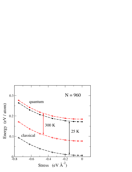
Figure 4: Dependence of the internal energy of graphene on tensile stress, as derived from classical (open symbols) and PIMD simulations (solid symbols) at two temperatures: 25 K (circles) and 300 K (squares). These results were obtained for a simulation cell including 960 carbon atoms. Vertical arrows indicate the increase in internal energy due to quantization of nuclear motion at each temperature. Error bars are less than the symbol size.

The internal energy $E$ is calculated as a sum of the kinetic $K$ and potential energy $V$ obtained from the simulations at a given temperature. In our simulations of graphene, $K$ and $V$ have been found to slightly increase with system size, and their convergence is rather fast. Thus, for cells in the order of 200 atoms the size effect in the internal energy is almost inappreciable when compared to the largest cells.Herrero and Ramírez (2016) The kinetic energy is associated to vibrational motion of carbon atoms (in-plane and out-of-plane), but the potential energy includes contributions due to atomic vibrations and to the elastic energy due to changes in the area $A$ of graphene at finite temperatures and applied stresses (see below).

In Fig. 4 we display the stress dependence of the internal energy, $E-E_{0}$, as derived from classical and PIMD simulations for system size $N$ = 960. Results are shown for $T$ = 25 K (circles) and 300 K (squares). Open and solid symbols correspond to classical and PIMD simulations, respectively. At $P=0$, the classical energy per atom is basically given by the vibrational energy $E_{\rm vib}^{\rm cl}=3k_{B}T$, as follows from the equipartition theorem in a harmonic approximation (HA). As the tensile stress is increased ($P$ more negative), the classical internal energy increases for a given temperature, due to the contribution of the elastic energy associated to a finite strain in the graphene lattice. The behavior of the quantum results shown in Fig. 4 is similar to the classical ones. The main difference is the increase in internal energy caused by quantization of the nuclear motion. For zero stress, this increase amounts to 165 meV/atom at 25 K and 107 meV/atom at 300 K. These shifts do not appreciably change in the stress region considered here, and in fact the difference between quantum and classical results appears to be nearly constant in the results shown in Fig. 4.

To analyze the different contributions to the internal energy, $E(T)$, we write

$$E(T)=E_{0}+E_{\rm el}(A)+E_{\rm vib}(A,T)\,.$$ (7)

In this expression $E_{\rm el}(A)$ is the elastic energy corresponding to an area $A$, and $E_{\rm vib}(A,T)$ is the vibrational energy of the system. Although not explicitly indicated, the area $A$ is a function of the stress $P$ and temperature $T$. Our simulations give $E(T)$, and using Eq. (7) we can then split the internal energy $E(T)-E_{0}$ into an elastic and a vibrational part. The vibrational contribution $E_{\rm vib}$ can in turn be split into kinetic and potential energy parts: $E_{\rm vib}=V_{\rm vib}+K$.

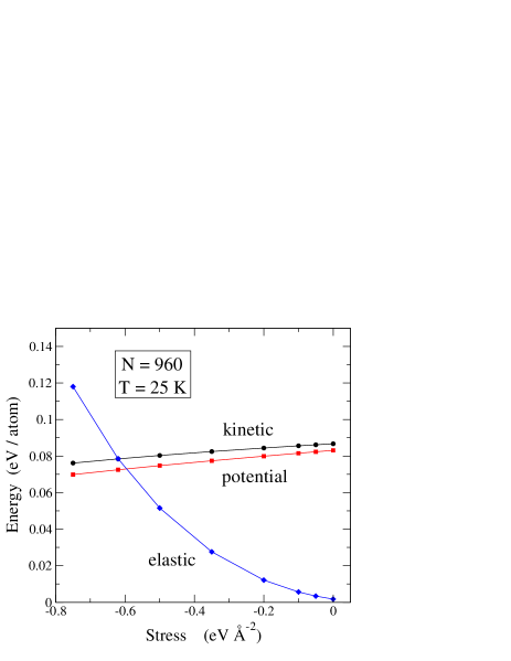
Figure 5: Different contributions to the internal energy of graphene, as functions of tensile stress. Symbols indicate results of PIMD simulations for $N$ = 960 atoms and $T$ = 25 K. Diamonds, elastic energy; circles, kinetic energy; squares, vibrational potential energy. Error bars are less than the symbol size. Lines are guides to the eye.

The elastic energy $E_{\rm el}(A)$ is defined here as the increase in energy corresponding to a strictly planar graphene layer with area $A$ respect to the minimum energy $E_{0}$. Thus, we have calculated $E_{\rm el}(A)$ for a supercell including 960 carbon atoms, expanding it isotropically and keeping it flat. Finite-size effects on the elastic energy are very small, and in fact negligible for our current purposes, as happens for the size dependence of the area $A$. For $A>A_{0}$, the elastic energy increases with $A$, and for small lattice expansion it can be approximated as $E_{\rm el}(A)\approx C(A-A_{0})^{2}$, with $C$ = 2.41 eV Å^-2. At room temperature ($T\sim$ 300 K) and for small stresses $P$ ($A$ close to $A_{0}$), the elastic energy is much smaller than the vibrational energy $E_{\rm vib}$, but this can be different for low $T$ and/or large applied stresses (see below). Once calculated the elastic energy for the area $A$ resulting from the simulations at given $T$ and $P$, we obtain the vibrational energy $E_{\rm vib}(A,T)$ by subtracting the elastic energy from the internal energy $E(T)$: $E_{\rm vib}=E(T)-E_{0}-E_{\rm el}(A)$ (see Eq. (7)). Then, the potential energy corresponding to vibrational motion, $V_{\rm vib}$, is found as $V_{\rm vib}=E_{\rm vib}-K$.

In Fig. 5 we present the different contributions to the internal energy of graphene vs. tensile stress, as derived from PIMD simulations for $N$ = 960 atoms and $T$ = 25 K. In this figure, diamonds represent the elastic energy, and circles and squares indicate $K$ and $V_{\rm vib}$, respectively. At $P=0$, $E_{\rm el}$ is close to zero, but slightly positive, as a consequence of the zero-point expansion of the graphene lattice, which causes that $A>A_{0}$. For increasing tensile stress, $E_{\rm el}$ rises and becomes similar to $K$ and $V_{\rm vib}$ for $P\approx-0.6$ eV Å^-2. At still larger tensile stress, the elastic contribution is the largest one, as shown in Fig. 5. For $T$ = 300 K the picture is qualitatively the same. The elastic energy increases roughly a constant value (26 meV/atom) with respect to the results at 25 K in the whole stress range shown in Fig. 5. The same happens for the kinetic energy, with a rise of 6 meV/atom. As a result, the crossing of $E_{\rm el}$ and $K$ at 300 K occurs for a tensile stress $P\approx-0.55$ eV Å^-2.

For a purely harmonic model for the vibrational modes, one expects $K=V_{\rm vib}$ (virial theoremLandau and Lifshitz (1980); Feynman (1972)), i.e., an energy ratio $K/V_{\rm vib}=1$ at any temperature in both classical and quantum approaches. This is not strictly the case for the results of our PIMD, because the vibrational amplitudes are finite, even at low temperatures, and feel the anharmonicity of the interatomic potential. In particular, we find $K>V_{\rm vib}$, for all temperatures and tensile stresses considered here. As displayed in Fig. 5 for $T$ = 25 K, the difference $K-V_{\rm vib}$ increases as the tensile stress is raised, so that $K$ is about 5% larger than $V_{\rm vib}$ for small stress, and around 9% larger for a stress of $-0.75$ eV Å^-2. Differences between the kinetic and potential contribution to the vibrational energy have been used for a quantification of the anharmonicity in condensed matter, as discussed earlier from path-integral simulations, e.g., for van der Waals solidsHerrero (2002) and H impurities in silicon.Herrero and Ramírez (1995)

Concerning the energy results for our quantum approach at low $T$, we note that analyses of anharmonicity in solids, based on quasiharmonic approximations and perturbation theory indicate that low-temperature changes in the vibrational energy with respect to a harmonic calculation are mostly due to the kinetic energy. Thus, considering perturbed harmonic oscillators with perturbations of type $x^{3}$ or $x^{4}$ at $T=0$, first-order changes in the energy are due to changes in $K$, and the potential energy stays unshifted in its unperturbed value.Landau and Lifshitz (1965); Herrero and Ramírez (1995)

V Out-of-plane motion

In this section we study the mean-square displacements of carbon atoms in the $z$ direction, normal to the graphene sheet, as obtained from our PIMD simulations. We mostly concentrate on the nature of these atomic displacements, i.e., if they can be well described by a classical model, or the C atoms appreciably behave as quantum particles. We expect of course that a classical description will lose accuracy as the temperature is reduced, but in the case of graphene it has been shown earlier that other factors such as the system size play also an important role in this question.Herrero and Ramírez (2016) Moreover, an external stress modifies the vibrational frequencies in the material, thus causing a change in the vibrational amplitudes and in the accuracy of a classical description at a given temperature.

PIMD simulations can be used to study vibrational amplitudes or atomic delocalization at finite temperatures. This includes a thermal (classical-like) motion, as well as a delocalization due to the quantum nature of the atomic nuclei, which can be quantified by the spacial extension of the paths associated to a given atomic nucleus. For each quantum path, we define the center-of-gravity (centroid) as

$$\overline{\bf r}_{i}=\frac{1}{N_{\rm Tr}}\sum_{j=1}^{N_{\rm Tr}}{\bf r}_{ij}\;,$$ (8)

where ${\bf r}_{ij}\equiv(x_{ij},y_{ij},z_{ij})$ is the 3D position of bead $j$ in the ring polymer associated to nucleus $i$. For the out-of-plane motion, we focus on the $z$-coordinate of the polymer beads. Then, the mean-square displacement $(\Delta z)^{2}_{i}$ of the atomic nucleus $i$ in the $z$ direction along a PIMD simulation run is defined as

$$(\Delta z)^{2}_{i}=\frac{1}{N_{\rm Tr}}\left<\sum_{j=1}^{N_{\rm Tr}}(z_{ij}-\left<\overline{z}_{i}\right>)^{2}\right>\,,$$ (9)

The kinetic energy of a particle is related to its quantum delocalization, or in the present context, to the spread of the paths associated to it. This can be measured by the mean-square radius-of-gyration of the ring polymers, with an out-of-plane component:Gillan (1988, 1990)

$$Q_{z,i}^{2}=\frac{1}{N_{\rm Tr}}\left<\sum_{j=1}^{N_{\rm Tr}}(z_{ij}-\overline{z}_{i})^{2}\right>\,.$$ (10)

The total spatial delocalization $(\Delta z)^{2}_{i}$ of atomic nucleus $i$ in the $z$ direction at a finite temperature includes, in addition to $Q_{z,i}^{2}$, another contribution which accounts for the classical-like motion of the centroid coordinate $\overline{z}_{i}$, i.e.

$$(\Delta z)^{2}_{i}=Q_{z,i}^{2}+C_{z,i}^{2}\,,$$ (11)

with

$$C_{z,i}^{2}=\left<\left(\overline{z}_{i}-\langle\overline{z}_{i}\rangle\right)^{2}\right>=\langle\overline{z}_{i}^{2}\rangle-\langle\overline{z}_{i}\rangle^{2}\,.$$ (12)

This term $C_{z,i}^{2}$ converges at high $T$ to the mean-square displacement $(\Delta z)^{2}_{i,{\rm cl}}$ given by a classical model, since in this limit each quantum path collapses onto a single point ($Q_{z,i}^{2}\to 0$). In the results presented below, we will show data for $(\Delta z)^{2}$, $Q_{z}^{2}$, and $C_{z}^{2}$, calculated as averages for the $N$ atoms in a simulation cell. For example:

$$(\Delta z)^{2}=\frac{1}{N}\sum_{i=1}^{N}(\Delta z)^{2}_{i}\,.$$ (13)

To connect the results of our simulations with the out-of-plane displacements corresponding to vibrational modes of the graphene sheet, we recall that the atomic mean-square displacement at temperature $T$ is given in a HA by

$$(\Delta z)^{2}_{\rm HA}=\frac{1}{N}\sum_{i,\bf k}\frac{\hbar}{2m\omega_{i}({\bf k})}\coth\left(\frac{\hbar\omega_{i}({\bf k})}{2k_{B}T}\right)\,,$$ (14)

where the index $i$ ($i$ = 1, 2) refers to the phonon bands ZA and ZO, with atomic displacements along the $z$ direction.Mounet and Marzari (2005); Karssemeijer and Fasolino (2011); Wirtz and Rubio (2004) The sum in ${\bf k}$ is extended to wavevectors ${\bf k}=(k_{x},k_{y})$ in the hexagonal Brillouin zone, with discrete ${\bf k}$ points spaced by $\Delta k_{x}=2\pi/L_{x}$ and $\Delta k_{y}=2\pi/L_{y}$.Ramírez et al. (2016) Eq. (14) has been used here to calculate $(\Delta z)^{2}_{\rm HA}$ in a harmonic approach. Increasing the system size $N$ causes the appearance of vibrational modes with longer wavelength $\lambda$. In fact, one has for the phonons an effective wavelength cut-off $\lambda_{max}\approx L$, with $L=(NA_{p})^{1/2}$, and the minimum wavevector is $k_{0}=2\pi/\lambda_{max}$, i.e., $k_{0}\sim N^{-1/2}$. For the calculations presented below, based on the formula in Eq. (14), we have used the vibrational frequencies in the phonon branches ZA and ZO obtained from diagonalization of the dynamical matrix corresponding to the LCBOPII potential employed here.

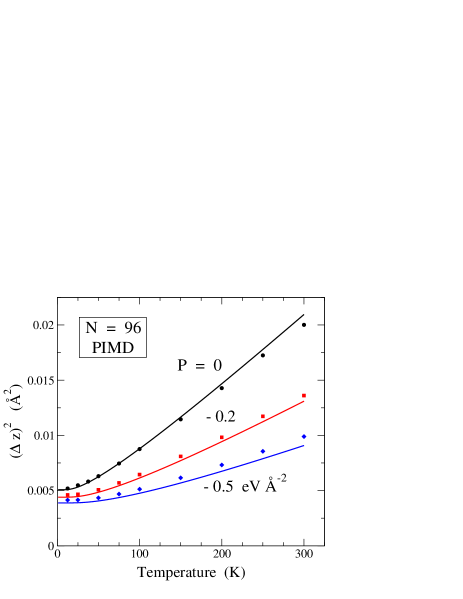
Figure 6: Mean-square displacement in the $z$ direction as a function of temperature, as derived from PIMD simulations for $N$ = 96 and $P$ = 0 (circles), $-0.2$ (squares), and $-0.5$ eV Å^-2 (diamonds). Error bars are in the order of the symbol size. Bold lines correspond to a harmonic approximation based on ZA and ZO vibrational modes.

For an applied stress $P$, the most important effect in the ZA and ZO bands is a change in frequency of the ZA modes in the low-frequency region, for which

$$\omega_{\rm ZA}({\bf k})^{2}=\omega^{0}_{\rm ZA}({\bf k})^{2}-\frac{P}{\rho}\,k^{2}$$ (15)

The zero-stress band $\omega^{0}_{\rm ZA}({\bf k})$ calculated for the minimum-energy structure (area $A_{0}$), verifies for small $k$: $\rho\,\omega^{0}_{\rm ZA}({\bf k})^{2}\approx\kappa k^{4}$. Then, for $P<0$ the small-$k$ region is dominated by the quadratic term (linear in $P$) in Eq. (15), so that $\omega_{\rm ZA}({\bf k})\approx\sqrt{-P/\rho}\;k$ for $k\ll$ 1 Å^-1.

In Fig. 6 we show results for the motion in the out-of-plane direction, obtained for a cell including 96 atoms. The use of a relatively small simulation cell is convenient to visualize the behavior of $(\Delta z)^{2}$ in the low-temperature region, where quantum effects are prominent. For larger cell sizes, these effects appear only at lower temperatures, which turns out to be difficult to observe from PIMD simulations.Herrero and Ramírez (2016) Solid symbols represent the mean-square displacement $(\Delta z)^{2}$ derived from the simulations, as a function of temperature for three different applied stresses: $P=0$ (circles), $-0.2$ (squares), and $-0.5$ eV Å^-2 (diamonds). Lines were calculated from a harmonic approximation based on the ZA and ZO phonon bands of graphene, as indicated above.

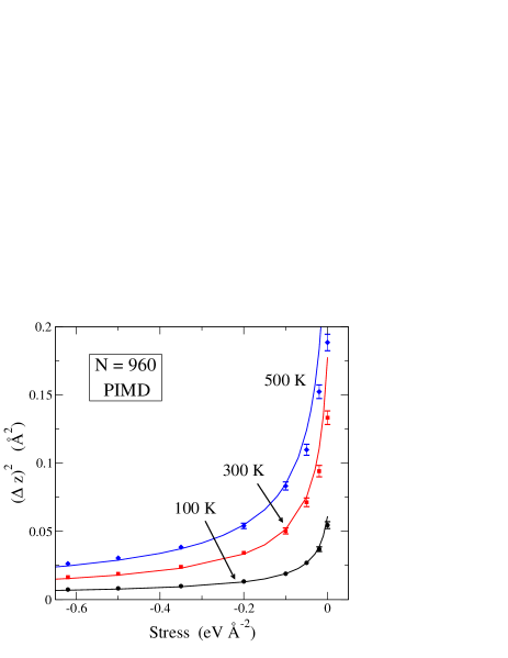
Figure 7: Mean-square displacement in the $z$ direction as a function of tensile stress, as derived from PIMD simulations for $N$ = 960 and three temperatures: $T$ = 500 K (diamonds), 300 K (squares), and 100 K (circles). Error bars, when not displayed, are in the order or less than the symbol size. Bold lines correspond to a harmonic approximation based on ZA and ZO vibrational modes.

One observes in Fig. 6 that the vibrational amplitude decreases as the tensile stress increases, mainly due to an increase in vibrational frequencies of ZA modes with low $k$ ($k\ll$ 1 Å^-1). This becomes important as the temperature is raised, but it is also appreciable in the low-temperature region, as shown in the figure. The lines derived from a HA are close to the results of the PIMD simulations at low temperature, but both sets of results depart progressively one from the other as temperature is raised. For $P=0$, $(\Delta z)^{2}_{\rm HA}<(\Delta z)^{2}_{\rm PI}$, but the opposite happens for $T>$ 100 K. For relatively large tensile stresses of $-0.2$ and $-0.5$ eV/Å^-2, we find $(\Delta z)^{2}_{\rm HA}<(\Delta z)^{2}_{\rm PI}$ in the whole temperature range presented in Fig. 6. For $T>300$ K, the difference between $(\Delta z)^{2}_{\rm PI}$ and $(\Delta z)^{2}_{\rm HA}$ steadily increases.

In Fig. 7 we display the mean-square displacements $(\Delta z)^{2}$ for $N=960$ as a function of applied stress $P$ for three temperatures: 100, 300, and 500 K. Symbols are results of PIMD simulations, whereas the lines correspond to the HA based on ZA and ZO vibrational modes. One observes first an important decrease in $(\Delta z)^{2}$ as the tensile stress is raised. This decrease is most appreciable for stresses in the range from 0 to $-0.1$ eV Å^-2. For larger stresses, the reduction of $(\Delta z)^{2}$ becomes slower. One also notices that the largest difference between $(\Delta z)^{2}_{\rm PI}$ and $(\Delta z)^{2}_{\rm HA}$ occurs for $P=0$, and it becomes smaller for larger pressure. For $P\sim-0.2$ eV Å^-2, both sets of results cross each other and the data derived from PIMD become slightly larger than those corresponding to the HA.

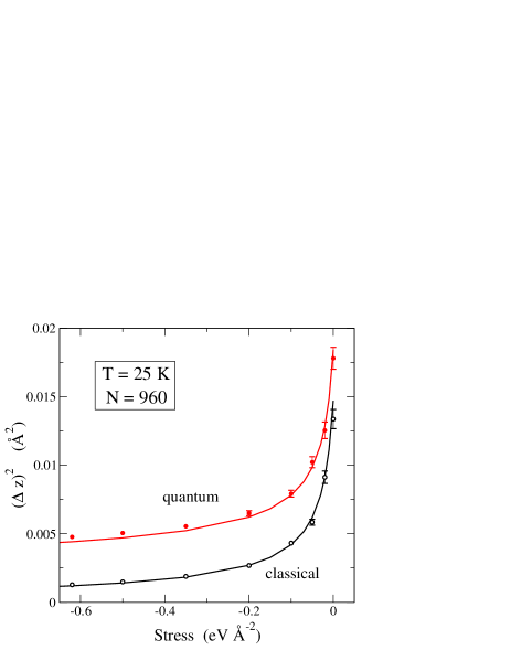
Figure 8: Mean-square displacement in the $z$ direction as a function of tensile stress, as derived from PIMD (solid circles) and classical (open circles) simulations for $N$ = 960 and $T$ = 25 K. Error bars, when not shown, are in the order or less than the symbol size. Lines were obtained from classical and quantum harmonic approximations based on ZA and ZO vibrational modes.

To get better insight into the influence of nuclear quantum effects on $(\Delta z)^{2}$ for different pressures, we have plotted in Fig. 8 the mean-square displacements as derived from classical MD (open circles) and PIMD (solid circles) simulations at 25 K. The lines were obtained from the HA described above for the quantum case [see Eq. (14)], and for the classical calculation we used the expression

$$C_{z,\rm HA}^{2}=\frac{1}{N}\sum_{i,\bf k}\frac{k_{B}T}{m\omega_{i}({\bf k})^{2}}\,.$$ (16)

One sees that the relevance of quantum effects increases for rising tensile stress, as can be measured from the ratio $(\Delta z)^{2}/C_{z}^{2}$ between the mean-square displacements in the quantum and classical case. In fact, this ratio goes from 1.3 for $P=0$ to 3.7 for $P=-0.6$ eV Å^-2. For a given stress, the difference between the quantum results for $(\Delta z)^{2}$ and the classical ones, $C_{z}^{2}$, decreases as temperature is raised. In fact, at $T=300$ K the mean-square displacement derived from PIMD simulations is about 10% larger than the classical result in the stress range displayed in Fig. 8.

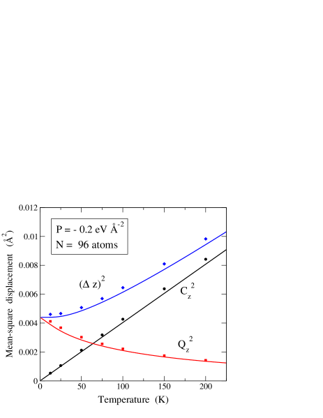
Figure 9: Temperature dependence of the mean-square displacement along the out-of-plane direction, $(\Delta z)^{2}$ (diamonds), along with its classical $C_{z}^{2}$ (circles) and quantum $Q_{z}^{2}$ (squares) contributions. These data correspond to PIMD simulations for a graphene cell containing 96 atoms and a tensile stress $P=-0.2$ eV Å^-2. Lines were obtained from a harmonic approximation based on ZA and ZO vibrational modes.

As indicated above, the mean-square displacement $(\Delta z)^{2}$ can be divided into two parts, $Q_{z}^{2}$ and $C_{z}^{2}$, the first one properly quantum in nature, measuring the extension of the quantum paths, and the second of a classical-like character, taking account of the centroid motion, i.e., global displacements of the paths. For the sake of comparing with the results of PIMD simulations, we have also calculated in the harmonic approximation $Q_{z,\rm HA}^{2}=(\Delta z)^{2}_{\rm HA}-C_{z,\rm HA}^{2}$, using Eqs. (14) and (16). To visualize the evolution of both terms as a function of temperature, we have plotted in Fig. 9 $(\Delta z)^{2}$ along with its two contributions $Q_{z}^{2}$ and $C_{z}^{2}$ for $N$ = 96 and a stress $P=-0.2$ eV Å^-2. In the limit $T\to 0$, $C_{z}^{2}$ vanishes and $Q_{z}^{2}$ converges to a value of about $4.5\times 10^{-3}$ Ų. $Q_{z}^{2}$ decreases for increasing temperature, as nuclear quantum effects become less relevant. On the contrary, the classical contribution $C_{z}^{2}$ increases with $T$, linearly in the HA [see Eq. (16)], and almost linearly for the results of PIMD simulations.

For the system size shown in Fig. 9 (N = 96), both contributions to $(\Delta z)^{2}$ are equal at $T\approx$ 64 K. At higher temperatures, the classical-like part $C_{z}^{2}$ is the main contribution to the atomic displacements in the $z$ direction. Values of $C_{z}^{2}$ given by PIMD simulations coincide within error bars with the mean-square atomic displacement obtained from classical MD simulations. The actual quantum delocalization can be estimated from the mean extension of the quantum paths in the $z$ direction, i.e., from $Q_{z}^{2}$. For $P=-0.2$ eV Å^-2, we find at 25 and 300 K an average extension $(\Delta z)_{Q}=(Q_{z}^{2})^{1/2}\approx$ 0.06 and 0.03 Å, respectively.

Figure 10: $P-T$ plane displaying the crossover from the region dominated by quantum delocalization ($Q_{z}^{2}>C_{z}^{2}$, below the lines) to the region dominated by classical-like motion ($C_{z}^{2}>Q_{z}^{2}$, above the lines). Data points were obtained from PIMD simulations for two system sizes: $N$ = 96 (circles) and 960 (squares). The lines were obtained from the HA discussed in the text.

The picture displayed in Fig. 9 for the atom displacements in the out-of-plane direction is qualitatively the same for different system sizes and applied stresses, but the temperature region where $Q_{z}^{2}$ or $C_{z}^{2}$ is the main contribution to $(\Delta z)^{2}$ as well as the crossing point $Q_{z}^{2}=C_{z}^{2}$ greatly depend on both variables $N$ and $P$. The dependence on $N$ is mainly caused by the enhancement of the classical-like contribution $C_{z}^{2}$ for increasing size, as observed earlier for results of classical MD simulations.Los et al. (2009); Gao and Huang (2014); Ramírez et al. (2016) The quantum contribution $Q_{z}^{2}$ has a small size effect and converges fast as $N$ is increased.Herrero and Ramírez (2016) For a given system size $N$, the ratio $Q_{z}^{2}/C_{z}^{2}$ decreases for increasing $T$ (see Fig. 9), and there is a crossover temperature $T_{c}(P)$ for which this ratio is unity. For $T>T_{c}(P)$ classical-like motion dominates the atomic motion in the $z$ direction.

In Fig. 10 we present $T_{c}$ as a function of the applied stress $P$ for two system sizes: $N$ = 96 and 960. Symbols are results derived from PIMD simulations and lines correspond to crossover temperatures derived from the HA based on the ZA and ZO phonon bands. Below the lines we have $Q_{z}^{2}>C_{z}^{2}$, i.e. the quantum contribution dominates in $(\Delta z)^{2}$, and the opposite happens above the lines with classical-like motion dominating the out-of-plane displacements. The crossover temperature $T_{c}$ depends on the system size $N$, since the effective low-energy cutoff scales as $k_{0}\sim N^{-1/2}$. This means that for a given stress $P$, an increase in $N$ causes the appearance of ZA modes with lower frequencies, which contribute to reduce $T_{c}$ (for a given $\omega$, the classical behavior dominates for $T\gtrsim\hbar\omega/k_{B}$).

The main limitations of the HA are the neglect of anharmonicity in the transverse vibrational modes, which is expected to be reasonably small at low $T$, and the use of Eq. (15) for ZA mode frequencies under stress. This equation, giving $\omega_{\rm ZA}({\bf k})^{2}$ as a sum of a zero-stress term, $\omega^{0}_{\rm ZA}({\bf k})^{2}$, and a term linear in the applied stress, $Pk^{2}/\rho$, is expected to be valid for small-$k$ ZA modes, which dominate the mean-square displacement of C atoms in the transverse direction to the graphene plane. Taking into account these limitations, the harmonic model captures qualitatively, and almost quantitatively, the basic aspects of the competition between classical-like and quantum dynamics of the C atoms in the $z$ direction.

VI Summary

We have presented results of PIMD simulations of a graphene monolayer at several temperatures and tensile stresses. The importance of quantum effects has been quantified by comparing results of such quantum simulations with those obtained from classical MD simulations. Structural variables are found to change when quantum nuclear motion is taken into account, especially at low temperatures. Thus, the sheet area and interatomic distances change appreciably in the range of temperatures and stresses considered here.

The LCBOPII potential model was shown earlier to give a reliable description of structural and thermodynamic properties of graphene. We have investigated here its reliability to describe nuclear quantum effects in the presence of a tensile stress. The results obtained in the simulations have allowed us to analyze both the in-plane $A_{p}$ and real area $A$ of graphene as functions of $T$ and $P$. The difference $A-A_{p}$ grows (decreases) as temperature (stress) is raised. The thermal contraction of $A_{p}$ becomes less important as the tensile stress increases and the amplitude of out-of-plane vibrations decreases. We emphasize that PIMD simulations yield a negative thermal expansion of $A_{p}$ at low $T$ for pressures so high as $-0.5$ eV Å^-2 ($-8$ N/m). On the contrary, in classical calculations this thermal expansion becomes positive at much smaller stresses.

Zero-point expansion of the graphene layer due to nuclear quantum effects is not negligible, and it amounts to an increase of about 1% in the area $A$. This zero-point effect is reduced for rising tensile stress. Moreover, the temperature dependence of the in-plane area $A_{p}$ is qualitatively different when derived from PIMD or classical simulations, even at temperatures between 300 and 1000 K. Such a difference appears for all tension stresses considered here, up to $P=-0.5$ eV Å^-2.

Atomic vibrations in the out-of-plane $z$ direction have been particularly considered, as they are important for the area $A_{p}$ and for the relative stability of the planar graphene layer vs. crumpling. Quantum effects are dominant for these vibrational modes provided that $k_{B}T<\hbar\omega$. However, the actual atomic motion at any finite temperature, resulting from the sum of mode contributions, is dominated by the classical thermal contribution as soon as the system size is large enough. This size effect appears in the quantum simulations at low temperatures, as a result of the presence of vibrational modes in the ZA band with smaller wavenumbers (frequencies) for larger graphene cells. In this respect, an interesting result is that the temperature region where quantum motion is dominant is enhanced by an external tensile stress, as shown in Fig. 10, i.e., for a given system size $T_{c}$ increases as the stress is raised.

An important point related to the consistency of the simulation results is their agreement with the principles of thermodynamics, in particular with the third law. This means that thermal expansion coefficients should converge to zero for $T\to 0$. We have found that this requirement is verified by both the in-plane area $A_{p}$ and the real area $A$ obtained from PIMD simulations for $P=0$ and $P<0$ (tensile stress).

An analysis of graphene under tensile stresses larger than those considered here may be interesting for its effect on mechanical, electronic, and optical properties. Such a study can be hindered by limitations associated to effective potentials at large strains, and would require the use of ab-initio methods (e.g., density-functional theory). An efficient combination of these methods with path-integral simulations is still restricted to cell sizes relatively small, a limitation that is expected to be progressively overcome in the forthcoming years.

Appendix A Pressure estimator

The Cartesian coordinates of the $N$ atomic nuclei in the crystalline membrane are denoted as ${\bf r}_{ij}$, where the $i=1,...,N$ indicates the atom, and $j=1,...,N_{\rm Tr}$ refers to the bead number. The staging coordinates ${\bf u}_{ij}$ are defined by a linear transformation of ${\bf r}_{ij}$ that diagonalizes the harmonic energy associated to the effective interactions between neighboring beads:Tuckerman and Hughes (1998); Tuckerman (2002)

$${\bf u}_{i1}={\bf r}_{i1}\;,$$ (17)

$${\bf u}_{ij}={\bf r}_{ij}-\frac{j-1}{j}{\bf r}_{i,j+1}-\frac{1}{j}{\bf r}_{i1}\;,\;\;j=2,\dots,N_{\rm Tr}\;.$$ (18)

The estimator of the 2D stress tensor ${\bf\tau}$ is similar to that employed in previous work for 3D systems.(Ramírez et al., 2008; Herrero and Ramírez, 2014) For PIMD simulations, its components are given by expressions such asTuckerman and Hughes (1998)

$$\tau_{xy}=\left\langle\frac{1}{A_{p}}\left(\sum_{i=1}^{N}\sum_{j=1}^{N_{\rm Tr}}\left(m_{j}v_{ij,x}v_{ij,y}-2k_{j}u_{ij,x}u_{ij,y}\right)-\frac{1}{N_{\rm Tr}}\sum_{j=1}^{N_{\rm Tr}}\frac{\partial U({\bf r}_{1j},\dots,{\bf r}_{Nj})}{\partial\epsilon_{xy}}\right)\right\rangle\;,$$ (19)

where the brackets $\langle\cdots\rangle$ indicate an ensemble average, $m_{j}$ is the dynamic mass associated to the staging coordinate ${\bf u}_{ij}$, $v_{ij,x}$, $v_{ij,y}$ are components of its corresponding velocity, and $\epsilon_{xy}$ is an element of the 2D strain tensor. The masses $m_{j}$ are given byTuckerman and Hughes (1998); Tuckerman (2002); Herrero and Ramírez (2014)

$$m_{1}=m\;,$$ (20)

$$m_{j}=\frac{j}{j-1}m\;,\;\;j=2,\dots,N_{\rm Tr}\;,$$ (21)

where $m$ is the nuclear mass. The constant $k_{j}$ is given for each bead $j$ by $k_{j}=m_{j}N_{\rm Tr}/2\beta^{2}\hbar^{2}$ for $j>1$ and $k_{1}=0$ ($\beta=(k_{B}T)^{-1}$).

The stress $P$ used in our PIMD simulations is

$$P=\frac{1}{2}\left(\tau_{xx}+\tau_{yy}\right)\,,$$ (22)

or $P=\langle{\cal P}\rangle$ with the estimator

$${\cal P}=\frac{1}{2A_{p}}\sum_{i=1}^{N}\sum_{j=1}^{N_{\rm Tr}}m_{j}\left(v_{ij,x}^{2}+v_{ij,y}^{2}\right)-\frac{E_{h}}{A_{p}}\\ -\frac{1}{N_{\rm Tr}}\sum_{j=1}^{N_{\rm Tr}}\frac{\partial U({\bf r}_{1j},\dots,{\bf r}_{Nj})}{\partial A_{p}}\;.$$ (23)

$E_{h}$ is the in-plane harmonic energy, that in terms of staging coordinates can be written as

$$E_{h}=\sum_{i=1}^{N}\sum_{j=2}^{N_{\rm Tr}}k_{j}\left(u_{ij,x}^{2}+u_{ij,y}^{2}\right)\;.$$ (24)

The last term in Eq. (23) is a sum of derivatives of the potential energy $U$ at different imaginary times (beads) $j$. In the present case of graphene, these derivatives were carried out analytically.

References

- Geim and Novoselov (2007) A. K. Geim and K. S. Novoselov, Nature Mater. 6, 183 (2007).
- Castro Neto et al. (2009) A. H. Castro Neto, F. Guinea, N. M. R. Peres, K. S. Novoselov, and A. K. Geim, Rev. Mod. Phys. 81, 109 (2009).
- Flynn (2011) G. W. Flynn, J. Chem. Phys. 135, 050901 (2011).
- Roldan et al. (2017) R. Roldan, L. Chirolli, E. Prada, J. Angel Silva-Guillen, P. San-Jose, and F. Guinea, Chem. Soc. Rev. 46, 4387 (2017).
- Ghosh et al. (2008) S. Ghosh, I. Calizo, D. Teweldebrhan, E. P. Pokatilov, D. L. Nika, A. A. Balandin, W. Bao, F. Miao, and C. N. Lau, Appl. Phys. Lett. 92, 151911 (2008).
- Nika et al. (2009) D. L. Nika, E. P. Pokatilov, A. S. Askerov, and A. A. Balandin, Phys. Rev. B 79, 155413 (2009).
- Balandin (2011) A. A. Balandin, Nature Mater. 10, 569 (2011).
- Lee et al. (2008) C. Lee, X. Wei, J. W. Kysar, and J. Hone, Science 321, 385 (2008).
- Seol et al. (2010) J. H. Seol, I. Jo, A. L. Moore, L. Lindsay, Z. H. Aitken, M. T. Pettes, X. Li, Z. Yao, R. Huang, D. Broido, et al., Science 328, 213 (2010).
- Prasher (2010) R. Prasher, Science 328, 185 (2010).
- Herrero and Ramírez (2016) C. P. Herrero and R. Ramírez, J. Chem. Phys. 145, 224701 (2016).
- Fasolino et al. (2007) A. Fasolino, J. H. Los, and M. I. Katsnelson, Nature Mater. 6, 858 (2007).
- Meyer et al. (2007) J. C. Meyer, A. K. Geim, M. I. Katsnelson, K. S. Novoselov, T. J. Booth, and S. Roth, Nature 446, 60 (2007).
- de Andres et al. (2012a) P. L. de Andres, F. Guinea, and M. I. Katsnelson, Phys. Rev. B 86, 144103 (2012a).
- Evans and Rawicz (1990) E. Evans and W. Rawicz, Phys. Rev. Lett. 64, 2094 (1990).
- Safran (1994) S. A. Safran, Statistical Thermodynamics of Surfaces, Interfaces, and Membranes (Addison Wesley, New York, 1994).
- Cerda and Mahadevan (2003) E. Cerda and L. Mahadevan, Phys. Rev. Lett. 90, 074302 (2003).
- Wong and Pellegrino (2006) Y. W. Wong and S. Pellegrino, J. Mech. Materials Struct. 1, 3 (2006).
- Kirilenko et al. (2011) D. A. Kirilenko, A. T. Dideykin, and G. Van Tendeloo, Phys. Rev. B 84, 235417 (2011).
- Nicholl et al. (2015) R. J. T. Nicholl, H. J. Conley, N. V. Lavrik, I. Vlassiouk, Y. S. Puzyrev, V. P. Sreenivas, S. T. Pantelides, and K. I. Bolotin, Nature Commun. 6, 8789 (2015).
- Ruiz-Vargas et al. (2011) C. S. Ruiz-Vargas, H. L. Zhuang, P. Y. Huang, A. M. van der Zande, S. Garg, P. L. McEuen, D. A. Muller, R. G. Hennig, and J. Park, Nano Lett. 11, 2259 (2011).
- Kosmrlj and Nelson (2013) A. Kosmrlj and D. R. Nelson, Phys. Rev. E 88, 012136 (2013).
- Kosmrlj and Nelson (2014) A. Kosmrlj and D. R. Nelson, Phys. Rev. E 89, 022126 (2014).
- Ramírez and Herrero (2017) R. Ramírez and C. P. Herrero, Phys. Rev. B 95, 045423 (2017).
- López-Polín et al. (2017) G. López-Polín, M. Jaafar, F. Guinea, R. Roldán, C. Gómez-Navarro, and J. Gómez-Herrero, Carbon 124, 42 (2017).
- Pozzo et al. (2011) M. Pozzo, D. Alfè, P. Lacovig, P. Hofmann, S. Lizzit, and A. Baraldi, Phys. Rev. Lett. 106, 135501 (2011).
- Woods et al. (2014) C. R. Woods, L. Britnell, A. Eckmann, R. S. Ma, J. C. Lu, H. M. Guo, X. Lin, G. L. Yu, Y. Cao, R. V. Gorbachev, et al., Nature Phys. 10, 451 (2014).
- Amorim et al. (2016) B. Amorim, A. Cortijo, F. de Juan, A. G. Grushine, F. Guinea, A. Gutierrez-Rubio, H. Ochoa, V. Parente, R. Roldan, P. San-Jose, et al., Phys. Rep. 617, 1 (2016).
- Shimojo et al. (2008) F. Shimojo, R. K. Kalia, A. Nakano, and P. Vashishta, Phys. Rev. B 77, 085103 (2008).
- de Andres et al. (2012b) P. L. de Andres, F. Guinea, and M. I. Katsnelson, Phys. Rev. B 86, 245409 (2012b).
- Chechin et al. (2014) G. M. Chechin, S. V. Dmitriev, I. P. Lobzenko, and D. S. Ryabov, Phys. Rev. B 90, 045432 (2014).
- Herrero and Ramírez (2009) C. P. Herrero and R. Ramírez, Phys. Rev. B 79, 115429 (2009).
- Cadelano et al. (2009) E. Cadelano, P. L. Palla, S. Giordano, and L. Colombo, Phys. Rev. Lett. 102, 235502 (2009).
- Akatyeva and Dumitrica (2012) E. Akatyeva and T. Dumitrica, J. Chem. Phys. 137, 234702 (2012).
- Lee et al. (2013) G.-D. Lee, E. Yoon, N.-M. Hwang, C.-Z. Wang, and K.-M. Ho, Appl. Phys. Lett. 102, 021603 (2013).
- Shen et al. (2013) H.-S. Shen, Y.-M. Xu, and C.-L. Zhang, Appl. Phys. Lett. 102, 131905 (2013).
- Los et al. (2009) J. H. Los, M. I. Katsnelson, O. V. Yazyev, K. V. Zakharchenko, and A. Fasolino, Phys. Rev. B 80, 121405 (2009).
- Ramírez et al. (2016) R. Ramírez, E. Chacón, and C. P. Herrero, Phys. Rev. B 93, 235419 (2016).
- Magnin et al. (2014) Y. Magnin, G. D. Foerster, F. Rabilloud, F. Calvo, A. Zappelli, and C. Bichara, J. Phys.: Condens. Matter 26, 185401 (2014).
- Los et al. (2016) J. H. Los, A. Fasolino, and M. I. Katsnelson, Phys. Rev. Lett. 116, 015901 (2016).
- Gillan (1988) M. J. Gillan, Phil. Mag. A 58, 257 (1988).
- Ceperley (1995) D. M. Ceperley, Rev. Mod. Phys. 67, 279 (1995).
- Brito et al. (2015) B. G. A. Brito, L. Cândido, G.-Q. Hai, and F. M. Peeters, Phys. Rev. B 92, 195416 (2015).
- Mounet and Marzari (2005) N. Mounet and N. Marzari, Phys. Rev. B 71, 205214 (2005).
- Shao et al. (2012) T. Shao, B. Wen, R. Melnik, S. Yao, Y. Kawazoe, and Y. Tian, J. Chem. Phys. 137, 194901 (2012).
- Gao and Huang (2014) W. Gao and R. Huang, J. Mech. Phys. Solids 66, 42 (2014).
- Feynman (1972) R. P. Feynman, Statistical Mechanics (Addison-Wesley, New York, 1972).
- Kleinert (1990) H. Kleinert, Path Integrals in Quantum Mechanics, Statistics and Polymer Physics (World Scientific, Singapore, 1990).
- Chandler and Wolynes (1981) D. Chandler and P. G. Wolynes, J. Chem. Phys. 74, 4078 (1981).
- Herrero and Ramírez (2014) C. P. Herrero and R. Ramírez, J. Phys.: Condens. Matter 26, 233201 (2014).
- Los et al. (2005) J. H. Los, L. M. Ghiringhelli, E. J. Meijer, and A. Fasolino, Phys. Rev. B 72, 214102 (2005).
- Ghiringhelli et al. (2005a) L. M. Ghiringhelli, J. H. Los, A. Fasolino, and E. J. Meijer, Phys. Rev. B 72, 214103 (2005a).
- Zakharchenko et al. (2009) K. V. Zakharchenko, M. I. Katsnelson, and A. Fasolino, Phys. Rev. Lett. 102, 046808 (2009).
- Ghiringhelli et al. (2005b) L. M. Ghiringhelli, J. H. Los, E. J. Meijer, A. Fasolino, and D. Frenkel, Phys. Rev. Lett. 94, 145701 (2005b).
- Politano et al. (2012) A. Politano, A. R. Marino, D. Campi, D. Farías, R. Miranda, and G. Chiarello, Carbon 50, 4903 (2012).
- Lambin (2014) P. Lambin, Appl. Sci. 4, 282 (2014).
- Sfyris et al. (2015) D. Sfyris, E. N. Koukaras, N. Pugno, and C. Galiotis, J. Appl. Phys. 118, 075301 (2015).
- Memarian et al. (2015) F. Memarian, A. Fereidoon, and M. D. Ganji, Superlattices Microstruct. 85, 348 (2015).
- Zou et al. (2016) J.-H. Zou, Z.-Q. Ye, and B.-Y. Cao, J. Chem. Phys. 145, 134705 (2016).
- Anastasi et al. (2016) A. A. Anastasi, K. Ritos, G. Cassar, and M. K. Borg, Mol. Simul. 42, 1502 (2016).
- Ghasemi and Rajabpour (2017) H. Ghasemi and A. Rajabpour, J. Phys. Conf. Series 785, 012006 (2017).
- Tuckerman et al. (1992) M. E. Tuckerman, B. J. Berne, and G. J. Martyna, J. Chem. Phys. 97, 1990 (1992).
- Tuckerman and Hughes (1998) M. E. Tuckerman and A. Hughes, in Classical and Quantum Dynamics in Condensed Phase Simulations, edited by B. J. Berne, G. Ciccotti, and D. F. Coker (Word Scientific, Singapore, 1998), p. 311.
- Martyna et al. (1999) G. J. Martyna, A. Hughes, and M. E. Tuckerman, J. Chem. Phys. 110, 3275 (1999).
- Tuckerman (2002) M. E. Tuckerman, in Quantum Simulations of Complex Many–Body Systems: From Theory to Algorithms, edited by J. Grotendorst, D. Marx, and A. Muramatsu (NIC, FZ Jülich, 2002), p. 269.
- Herman et al. (1982) M. F. Herman, E. J. Bruskin, and B. J. Berne, J. Chem. Phys. 76, 5150 (1982).
- Herrero et al. (2006) C. P. Herrero, R. Ramírez, and E. R. Hernández, Phys. Rev. B 73, 245211 (2006).
- Herrero and Ramírez (2011) C. P. Herrero and R. Ramírez, J. Chem. Phys. 134, 094510 (2011).
- Ramírez et al. (2012) R. Ramírez, N. Neuerburg, M. V. Fernández-Serra, and C. P. Herrero, J. Chem. Phys. 137, 044502 (2012).
- Ramírez et al. (2008) R. Ramírez, C. P. Herrero, E. R. Hernández, and M. Cardona, Phys. Rev. B 77, 045210 (2008).
- Fournier and Barbetta (2008) J.-B. Fournier and C. Barbetta, Phys. Rev. Lett. 100, 078103 (2008).
- Imparato (2006) A. Imparato, J. Chem. Phys. 124, 154714 (2006).
- Waheed and Edholm (2009) Q. Waheed and O. Edholm, Biophys. J. 97, 2754 (2009).
- Chacón et al. (2015) E. Chacón, P. Tarazona, and F. Bresme, J. Chem. Phys. 143, 034706 (2015).
- Nicholl et al. (2017) R. J. T. Nicholl, N. V. Lavrik, I. Vlassiouk, B. R. Srijanto, and K. I. Bolotin, Phys. Rev. Lett. 118, 266101 (2017).
- Hahn et al. (2016) K. R. Hahn, C. Melis, and L. Colombo, J. Phys. Chem. C 120, 3026 (2016).
- Michel et al. (2015) K. H. Michel, S. Costamagna, and F. M. Peeters, Phys. Status Solidi B 252, 2433 (2015).
- Landau and Lifshitz (1980) L. D. Landau and E. M. Lifshitz, Statistical Physics (Pergamon, Oxford, 1980), 3rd ed.
- Herrero (2002) C. P. Herrero, Phys. Rev. B 65, 014112 (2002).
- Herrero and Ramírez (1995) C. P. Herrero and R. Ramírez, Phys. Rev. B 51, 16761 (1995).
- Landau and Lifshitz (1965) L. D. Landau and E. M. Lifshitz, Quantum Mechanics (Pergamon, Oxford, 1965), 2nd ed.
- Gillan (1990) M. J. Gillan, in Computer Modelling of Fluids, Polymers and Solids, edited by C. R. A. Catlow, S. C. Parker, and M. P. Allen (Kluwer, Dordrecht, 1990), p. 155.
- Karssemeijer and Fasolino (2011) L. J. Karssemeijer and A. Fasolino, Surf. Sci. 605, 1611 (2011).
- Wirtz and Rubio (2004) L. Wirtz and A. Rubio, Solid State Commun. 131, 141 (2004).