Holographic conductivity of holographic superconductors with higher order corrections

Abstract

We analytically as well as numerically disclose the effects of the higher order correction terms in the gravity and in the gauge field on the properties of $s$-wave holographic superconductors. On the gravity side, we consider the higher curvature Gauss-Bonnet corrections and on the gauge field side, we add a quadratic correction term to the Maxwell Lagrangian. We show that for this system, one can still obtain an analytical relation between the critical temperature and the charge density. We also calculate the critical exponent and the condensation value both analytically and numerically. We use a variational method, based on the Sturm-Liouville eigenvalue problem for our analytical study, as well as a numerical shooting method in order to compare with our analytical results. For a fixed value of the Gauss-Bonnet parameter, we observe that the critical temperature decreases with increasing the nonlinearity of the gauge field. This implies that the nonlinear correction term to the Maxwell electrodynamics make the condensation harder. We also study the holographic conductivity of the system and disclose the effects of Gauss-Bonnet and nonlinear parameters $\alpha$ and $b$ on the superconducting gap. We observe that for various values of $\alpha$ and $b$, the real part of conductivity is proportional to the frequency per temperature, $\omega/T$, as frequency is enough large. Besides, the conductivity has a minimum in the imaginary part which is shifted toward greater frequency with decreasing the temperature.

1 Introduction

The correspondence between the gravity in a $d$-dimensional anti-de Sitter (AdS) spacetime and the conformal field theory (CFT) residing on the ($d-1$)-dimensional boundary of this spacetime, well-known as AdS/CFT correspondence, provides an established method for calculating correlation functions in a strongly interacting field theory using a dual classical gravity description [1]. It has been confirmed that this duality can be applied for solving the problem of high temperature superconductors in condensed matter physics [2]. This is due to the fact the high temperature superconductors are basically in a strong coupling regime, and thus one expects that the holographic method could give some insights into the pairing mechanism in these systems. Understanding the mechanism of high temperatures superconductors has long been a mysteries problem in modern condensed matter physics. Recently, it was suggested that it is logical to understand the properties of high temperature superconductors on the boundary of spacetime by considering a classical general relativity in one higher dimensions. This idea is called the holographic superconductors (HSC) [3, 4, 5] and has got a lot of attentions in the past decade. According to the HSC proposal, in the gravity side, a Maxwell field and a charged scalar field are introduced to describe the $U(1)$ symmetry and the scalar operator in the dual field theory, respectively. This holographic model undergoes a phase transition from black hole with no hair (normal phase/conductor phase) to the case with scalar hair at low temperatures (superconducting phase) [6].

Nowadays, the investigations on the HSC have attracted considerable attention and become an active field of research. Let us review some works in this direction. In the background of Schwarzschild AdS black holes in Einstein gravity, the properties of HSC have been explored in [7, 8, 9, 10, 11, 12, 13, 14]. The studies were also generalized to higher order gravity theories such as Gauss-Bonnet gravity [15, 16, 17, 18, 19]. It was argued that the critical temperature of the HSC decreases with increasing the backreaction, although the effect of the Gauss-Bonnet coupling is more subtle: the critical temperature first decreases then increases as the coupling tends towards the Chern-Simons value in a backreaction dependent fashion [18]. It was confirmed that the critical exponent of the condensation in Gauss-Bonnet HSC still obeys the mean field theory and has the value $1/2$ [17]. Other studies on the holographic superconductor have been carried out in (see for example [20, 21, 22, 23, 24, 25, 26, 27, 28, 29, 30, 31, 32, 33, 34, 35, 36, 37, 38, 39, 40, 41, 42, 43, 44, 45] and references therein).

It is also interesting to investigate the electrical conductivity of HSC in the dual CFT as a function of frequency. In the AdS/CFT correspondence, the electrical conductivity can be computed by looking at the linear response of the system to fluctuations of the fields $A_{x}$ and $g_{tx}$ in the bulk. These fluctuations are dual to the electric current $J_{x}$ and energy current $T_{tx}$ operators in the CFT. In the context of linear Maxwell field, the conductivity of HSC were computed in [2, 4, 5]. In the presence of nonlinear electrodynamics, the conductivity of HSC have been investigated in [46, 47]. Also, in the context of Born-Infeld nonlinear electrodynamics, the optical properties of Lifshitz HSC has been explored in [48]. It was demonstrated that this superconductor exhibits metamatrial property in low frequency of the external electric field for certain region of nonlinear parameter. The effects of the Weyle coupling parameter and Lifshitz dynamic exponent on the conductivity of HSC have been explored in [49]. In Ref. [50], a rotating BTZ black holes was considered as the gravity dual to $(1+1)$ dimensional superconductor. In this case, depending of the angular momentum on the conductivity has been investigated. Recently, the authors of [51] have analytically computed the holographic conductivity of HSC in the presence of Born-Infeld nonlinear electrodynamic by considering the backreaction of the matter field on the bulk metric. Further investigations on the holographic conductivity of HSC have been performed in [52, 53].

In this work, we will address the effects of the higher order corrections on the holographic conductivity of the $s$-wave HSC. On the gravity side, we will consider the Gauss-Bonnet curvature correction terms which is most general action in the 5D spacetime and on the gauge field side we add the quadratic nonlinear gauge term. We shall investigate the effects of these correction terms on the imaginary and real parts of the electrical conductivity of the system. With these correction terms, especially including a Gauss-Bonnet correction to the 5D action, we have the most general action with second-order field equations in 5D [54], which provides the most general models for the $s$-wave HSC. Furthermore, in an effective action approach to the string theory, the Gauss-Bonnet term corresponds to the leading order quantum corrections to gravity, and its presence guarantees a ghost-free action[55]. The purpose of this work is to anallytically as well as numerically explore the effects of these correction terms on the properties of $s$-wave HSC.

The plan of the work is as follows. In section 2, we will set up our model of the HSC in Gauss-Bonnet gravity with nonlinear electrodynamics in the probe limit and drive the equations of motion. In section 3, we analytically as well as numerically compute the relationship between the critical temperature and the charge density of Gauss-Bonnet HSC. In section 4, we study condensation operator near the critical temperature using analytical and numerical method. In section 5 we investigate the electrical conductivity of the HSC in Gauss Bonnet gravity with nonlinear correction term to the Maxwell field. In particular, we shall find the ratio of the gap frequency in conductivity to the critical temperature. At last, we summarize and discuss our results in section 6.

2 HSC in Gauss-Bonnet gravity with nonlinear electrodynamics

We consider the 5D Einstein-Gauss-Bonnet gravity in the background of AdS spaces which is described by the action [56],

$$S=\int d^{5}x\sqrt{-g}\left[R-2\Lambda+\frac{\alpha}{2}\left(R^{2}-4R^{\mu\nu}R_{\mu\nu}+R^{\mu\nu\rho\sigma}R_{\mu\nu\rho\sigma}\right)+L_{M}\right],$$ (1)

where $\Lambda=-6/l^{2}$ is the cosmological constant of $5$-dimensional AdS spacetime with radius $l$, $\alpha$ is the Gauss-Bonnet coefficient with dimension $(\mathit{length})^{2}$, $R_{\mu\nu\rho\sigma}$, $R_{\mu\nu}$ and $R$ are the Riemann curvature tensor, Ricci tensor, and the Ricci scalar, respectively. For convenience, hereafter we set the AdS radius $l=1$. We consider the Lagrangian density of the matter field, $L_{M}$, as

$$L_{M}={L}_{NL}-|\nabla\psi-iqA\psi|^{2}-m^{2}|\psi|^{2}.$$ (2)

where $\psi$ is a scalar field, $q$ and $m$ are, respectively, the charge and the mass of the scalar field, and the Lagrangian density of the nonlinear electrodynamics is given by [57, 58]

$$\mathcal{L}_{\mathrm{NL}}=\mathcal{F}+b\mathcal{F}^{2}+O(\mathcal{F}^{4}),$$ (3)

where $\mathcal{F}=-\frac{1}{4}F^{\mu\nu}F_{\mu\nu}$ is the Maxwell Lagrangian and $b$ is a parameter. The term $b\mathcal{F}^{2}$ is the first order leading nonlinear correction term to the Maxwell field. There are several motivation for choosing the nonlinear Lagrangian in the form of (3). First, the series expansion of the three well-known Lagrangian of nonlinear electrodynamics such as Born-Infeld, Logarithmic and Exponential nonlinear electrodynamics have the form of (3) [59]. Second, calculating one-loop approximation of QED, it was shown [60] that the effective Lagrangian is given by (3). Besides, if one neglect all other gauge fields, one may arrive at the effective quadratic order of $U(1)$ as $\mathcal{F}^{2}$ [61, 62]. Furthermore, considering the next order correction terms in the heterotic string effective action one can obtain the $\mathcal{F}^{2}$ term as a corrections to the bosonic sector of supergravity, which has the same order as the Gauss-Bonnet term [61, 62, 63, 64],

$$L_{\mathrm{cor}}=\beta\left[\alpha\left(R^{2}-4R^{\mu\nu}R_{\mu\nu}+R^{\mu\nu\rho\sigma}R_{\mu\nu\rho\sigma}\right)+b(F^{\mu\nu}F_{\mu\nu})^{2}\right].$$ (4)

The field equations can be obtained by varying action (1) with respect to the metric $g_{\mu\nu}$, the scalar field $\psi$, and and the gauge field $A_{\mu}$. We find

$$R_{\mu\nu}-\frac{(R-2\Lambda)}{2}g_{\mu\nu}-\frac{\alpha}{2}\left\{\frac{1}{2}g_{\mu\nu}\left(R^{2}-4R^{\rho\sigma}R_{\rho\sigma}+R^{\kappa\lambda\rho\sigma}R_{\kappa\lambda\rho\sigma}\right)\right.$$

$$\left.-2RR_{\mu\nu}+4R_{\mu\lambda}R_{\ \nu}^{\lambda}+4R_{\mu\rho\nu\sigma}R^{\rho\sigma}-2R_{\mu}^{\ \rho\sigma\lambda}R_{\nu\rho\sigma\lambda}\right\}=T_{\mu\nu},$$ (5)

$$(\nabla_{\mu}-iqA_{\mu})(\nabla^{\mu}-iqA^{\mu})\psi-m^{2}\psi=0,$$ (6)

$$\nabla_{\mu}\left[\left(1+2b\mathcal{F}\right)F^{\mu\nu}\right]=iq\left[\psi^{\ast}(\nabla^{\nu}-iqA^{\nu})\psi-\psi(\nabla^{\nu}+iqA^{\nu})\psi^{\ast}\right],$$ (7)

where $T_{\mu\nu}$ is the matter-stress tensor

$$T_{\mu\nu}=\frac{1}{2}\left(\mathcal{F}+b\mathcal{F}^{2}\right)g_{\mu\nu}-2\left(1+2b\mathcal{F}\right)F_{\mu\rho}F_{\nu}^{\ \rho}-\frac{1}{2}m^{2}|\psi|^{2}g_{\mu\nu}-\frac{1}{2}g_{\mu\nu}|\nabla\psi-iqA\psi|^{2}$$

$$+\frac{1}{2}\left[(\nabla^{\nu}-iqA^{\nu})\psi(\nabla^{\mu}+iqA^{\mu})\psi^{\ast}+\mu\leftrightarrow\nu\right].$$ (8)

The metric of a planar Schwarzschild-AdS black hole in 5D is [65]

$$ds^{2}=-f(r)dt^{2}+\frac{dr^{2}}{f(r)}+r^{2}(dx^{2}+dy^{2}+dz^{2}),$$ (9)

with

$$f(r)=\frac{r^{2}}{2\alpha}\left(1-\sqrt{1-4\alpha\left(1-\frac{r_{+}^{4}}{r^{4}}\right)}\right).$$ (10)

The Hawking temperature at the horizon can be written in the form

$$T=\frac{f^{{}^{\prime}}(r)}{4\pi}=\frac{r_{+}}{\pi}.$$ (11)

It is worthwhile to note that in the limit $r\rightarrow\infty$, we can obtain

$$f(r)\sim\frac{r^{2}}{2\alpha}\left[1-\sqrt{1-4\alpha}\right],$$ (12)

so we can introduce the effective AdS radius as

$$L_{\mathrm{eff}}^{2}=\frac{2\alpha}{1-\sqrt{1-4\alpha}}.$$ (13)

We choose the gauge and the scalar fields in the form [2]

$$A_{\mu}=(\phi(r),0,0,0,0),~{}\ \ \ ~{}~{}~{}~{}\psi=\psi(r),$$ (14)

Inserting the metric (9) and the gauge and scalar fields (14) in the field equations (6) and (7), we arrive at

$$\partial_{r}^{2}\psi+\left(\frac{3}{r}+\frac{\partial_{r}f}{f}\right)\partial_{r}\psi+\left(\frac{\phi^{2}}{f^{2}}-\frac{m^{2}}{f}\right)\psi=0,$$ (15)

$$\partial_{r}^{2}\phi+\frac{3}{r}\left(1-2b(\partial_{r}\phi)^{2}\right)\partial_{r}\phi-\frac{2\psi^{2}\phi}{f}\left(1-3b(\partial_{r}\phi)^{2}\right)=0.$$ (16)

The horizon radius is defined as the root of $f(r_{+})=0$. The regularity condition for the gauge field $A_{t}$ on the horizon $r_{+}$, implies the boundary condition $\phi(r_{+})=0$, which substituting in Eq. (15) yields

$$\ ~{}~{}~{}~{}~{}\psi(r_{+})=\frac{\partial_{r}f(r_{+})}{m^{2}}\partial_{r}\psi(r_{+}).$$ (17)

Near the AdS boundary ($r\rightarrow\infty$) the asymptotic behaviors of the solutions are given by

$$\phi(r) = \mu-\frac{\rho}{r^{2}},$$ (18)

$$\psi(r) = \frac{\psi_{-}}{r^{\Delta_{-}}}+\frac{\psi_{+}}{r^{\Delta_{+}}},$$ (19)

where $\Delta_{\pm}=2\pm\sqrt{4+m^{2}L_{\mathrm{eff}}^{2}}$. It is clear that we should have $m^{2}L_{\mathrm{eff}}^{2}\geq-4$. The value of $\Delta_{\pm}$ depend on $\tilde{m}^{2}=m^{2}L_{\mathrm{eff}}^{2}$. For example, setting $\tilde{m}^{2}=-3$, we have $\Delta_{+}=3$ and $\Delta_{-}=1$. The coefficients $\psi_{\pm}$ correspond to the vacuum expectation values of the condensate operator, namely $\psi_{\pm}=<\mathcal{O_{\pm}}>$, where $\mathcal{O_{\pm}}$ is the dual operator to the scalar field with the conformal dimension $\Delta_{\pm}$. Following [2], we can impose the boundary condition in which either $\psi_{-}$ or $\psi_{+}$ vanishes, so that the theory is stable in the asymptotic AdS region. In what follow, we set $\psi_{-}=0$ and take $\psi_{+}=\langle\mathcal{O_{+}}\rangle$ non zero. The interpretation of the parameters $\mu$ and $\rho$, also comes from the gauge/gravity dictionary and are, respectively, interpreted as the chemical potential and charge density of the conformal field theory on the boundary.

3 Relation between critical temperature and charge density

In this section, we are going to study the critical temperature of HSC, when the higher order corrections to the gravity side as well as the gauge field is taken into account. We shall continue our study both analytically and numerically and compare the two method with each other.

3.1 Analytical method

Here, we analytically obtain the relation between the critical temperature and the charge density of Gauss-Bonnet HSC. To do this, we first transform the coordinate $r$ to $z$, such that $z={r_{+}}/{r}$. Using this new coordinates, the equations of motion (15) and (16) can be rewritten as

$$\partial_{z}^{2}\phi-\frac{1}{z}\partial_{z}\phi+\frac{6bz^{3}}{r_{+}^{2}}(\partial_{z}\phi)^{3}-\frac{2\psi^{2}\phi r_{+}^{2}}{fz^{4}}+\frac{6b(\partial_{z}\phi)^{2}\phi\psi^{2}}{f}=0,$$ (20)

$$\partial_{z}^{2}\psi+(\frac{\partial_{z}f}{f}-\frac{1}{z})\partial_{z}\psi+\frac{r_{+}^{2}}{z^{4}}(\frac{\phi^{2}}{f^{2}}-\frac{m^{2}}{f})\psi=0.$$ (21)

Near the critical temperature ($T=T_{c}$) we have $\psi=0$, and thus equation (20) reduces to

$$\partial_{z}^{2}\phi-\frac{1}{z}\partial_{z}\phi+\frac{6bz^{3}}{r_{+}^{2}}(\partial_{z}\phi)^{3}=0.$$ (22)

Solving the above equation for the small value of nonlinear parameter $b$, we find

$$\phi(z)=\lambda r_{+c}(1-z^{2})\left[1-\frac{b\lambda^{2}}{2}\xi(z)\right]+O(b^{2}),$$ (23)

where

$$\xi(z)=(1+z^{2})(1+z^{4}),~{}~{}~{}\ \ \ ~{}~{}~{}\lambda=\frac{\rho}{r_{+c}^{3}}.$$ (24)

Next, we consider the boundary conditions for $\psi$ near the critical point ($T\rightarrow T_{c}$). We assume $\psi$ has the following form [66]

$$\psi|_{z\rightarrow 0}\sim\frac{\langle\mathcal{O_{+}}\rangle}{r_{+}^{3}}z^{3}F(z),$$ (25)

where $F(z)$ is the trial function near the boundary $z=0$, which satisfies the boundary conditions $F(0)=1$ and $F^{\prime}(0)=0$. Substituting Eqs. (23) and (25) in Eq. (21) one arrives at

$$F^{{}^{\prime\prime}}+p(z)F^{{}^{\prime}}+q(z)F+\lambda^{2}w(z)F=0,$$ (26)

where the prime now indicates the derivative with respect to $z$, and $p(z)$, $q(z)$ and $w(z)$ read

$$p(z) = \frac{3(1-\sqrt{1-4\alpha+4\alpha z^{4}})-12\alpha+20\alpha z^{4}}{z[1-4\alpha+4\alpha z^{4}-\sqrt{1-4\alpha+4\alpha z^{4}}]},$$ (27)

$$q(z) = \frac{1}{z^{2}}\left[\frac{3(1-4\alpha-4\alpha z^{4}-\sqrt{1-4\alpha+4\alpha z^{4}})}{\sqrt{1-4\alpha+4\alpha z^{4}}-1+4\alpha-4\alpha z^{4}}+\frac{2m^{2}\alpha}{\sqrt{1-4\alpha+4\alpha z^{4}}-1}\right],$$ (28)

$$w(z) = \frac{4\alpha^{2}(1-z^{2})^{2}(1-\frac{b}{2}\lambda^{2}\xi(z))^{2}}{(1-\sqrt{1-4\alpha+4\alpha z^{4}})^{2}}.$$ (29)

It is a matter of calculations to convert Eq. (26) to the standard form of the Sturm-Liouville equation

$$(T(z)F^{{}^{\prime}}(z))^{{}^{\prime}}-Q(z)F(z)+\lambda^{2}P(z)F(z)=0,$$ (30)

where,

$$T(z) = \frac{z^{3}}{2\sqrt{\alpha}}(\sqrt{1-4\alpha+4\alpha z^{4}}-1)\approx z^{3}\sqrt{\alpha}(z^{4}-1)[1-\alpha(z^{4}-1)],$$ (31)

$$Q(z) = -T(z)q(z)\approx-3z\sqrt{\alpha}(3z^{4}+6\alpha z^{4}-7\alpha z^{8}),$$ (32)

$$P(z) = T(z)w(z)\approx\frac{\sqrt{\alpha}z^{3}(z^{2}-1)(1+\alpha(z^{4}-1))(1-\frac{b}{2}\lambda^{2}\xi(z))^{2}}{z^{2}+1}.$$ (33)

In the above equations we have only kept the terms up to order $\alpha^{3/2}$. Next, we perform a perturbative expansion $b\lambda^{2}$ and retain only the terms that are linear in $b$ such that

$$b\lambda^{2}=b(\lambda^{2}|_{b=0})+O(b^{2}),$$ (34)

where $\lambda^{2}|_{b=0}$ is the value of $\lambda^{2}$ for $b=0$. Thus we can rewrite Eq. (33) as

$$P(z)\approx\frac{\sqrt{\alpha}z^{3}(z^{2}-1)(1+\alpha(z^{4}-1))(1-b(\lambda^{2}|_{b=0})\xi(z))}{z^{2}+1}.$$ (35)

Employing the Sturm-Liouville eigenvalues problem, the eigenvalues of Eq. (30) can be obtained by varying the following function

$$\lambda^{2}=\frac{\int_{0}^{1}dz(T(z)(F^{{}^{\prime}}(z))^{2}+Q(z)F^{2}(z))}{\int_{0}^{1}dzP(z)F^{2}(z)},$$ (36)

where we also choose $F(z)=1-az^{2}$ and $m^{2}=-3/L_{\mathrm{eff}}^{2}$ to appraise this expression. At last, using Eqs. (11) and (24), for $T\sim T_{c}$, one can obtain

$$T_{c}=\zeta\rho^{1/3},$$ (37)

where $\zeta=\frac{1}{\pi\lambda_{\mathrm{min}}^{1/3}}$ and $\lambda_{\mathrm{min}}$ is the minimum eigenvalue which can be obtained by variation of Eq. (36). Our strategy, in the analytical method, for calculating the critical temperature for condensation is to minimize the function (36) with respect to the coefficient $a$ by fixing other parameters of the model such as $b$ and $\alpha$. Then, we obtain $\lambda_{\mathrm{min}}$ and hence the maximum value of $T_{c}/\rho^{1/3}$ can be deduced through relation (37). As an example, we bring the details of our calculation for $\alpha=0.01$ and $b=0.01$. In this case Eq. (36) reduces to

$$\lambda^{2}=\frac{0.150900-0.226000a+0.117119a^{2}}{0.003844-0.003350a+0.000911a^{2}},$$ (38)

whose minimum is $\lambda_{\mathrm{min}}=25.6427$ at $a=0.747087$. And thus according to Eq. (37), the critical temperature becomes $T_{c}=0.185363\rho^{1/3}$. In tables 1, 2 and 3, we summarize our results for $\lambda_{\mathrm{min}}$ and $\zeta$ for different values of the parameters $\alpha$, $a$ and $b$. This table shows that for a small and fixed value of $\alpha$, with increasing the nonlinear parameter $b$, the value of $\zeta=T_{c}/\rho^{1/3}$ decreases as well. As we shall see in the next section this results is in a very good agreement with the numerical results.

3.2 Numerical method

Now, we numerically investigate the critical behavior of the HSC in Gauss-Bonnet gravity with quadratic correction term to the gauge field. For the numerical study we employ the shooting method [67]. For simplicity we assume $r_{+}=1$, and thus Eqs. (20) and (21)for $\phi$ and $\psi$ reduces to

$$\partial_{z}^{2}\phi-\frac{1}{z}\partial_{z}\phi+6bz^{3}(\partial_{z}\phi)^{3}-\frac{2\psi^{2}\phi}{fz^{4}}+\frac{6b(\partial_{z}\phi)^{2}\phi\psi^{2}}{f}=0,$$ (39)

$$\partial_{z}^{2}\psi+\left(\frac{\partial_{z}f}{f}-\frac{1}{z}\right)\partial_{z}\psi+\frac{1}{z^{4}}\left(\frac{\phi^{2}}{f^{2}}-\frac{m^{2}}{f}\right)\psi=0.$$ (40)

Near the horizon ($z=1$), we can expand $\phi$ and $\psi$ as

$$\phi\approx\phi^{{}^{\prime}}(1)(1-z)+\frac{\phi^{{}^{\prime\prime}}(1)}{2}(1-z)^{2}+\dots,$$ (41)

$$\psi\approx\psi(1)+\psi^{{}^{\prime}}(1)(1-z)+\frac{\psi^{{}^{\prime\prime}}(1)}{2}(1-z)^{2}+\dots,$$ (42)

while near the AdS boundary ($z=0$), they behave like

$$\phi\approx\mu-\rho z^{2},$$ (43)

$$\psi\approx\psi_{-}z^{\Delta_{-}}+\psi_{+}z^{\Delta_{-}}.$$ (44)

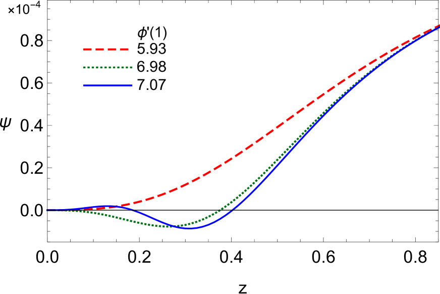
(a)  $\alpha=0.0001,b=0.01$

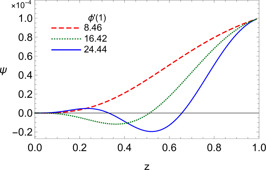
(b)  $\alpha=0.01,b=0$

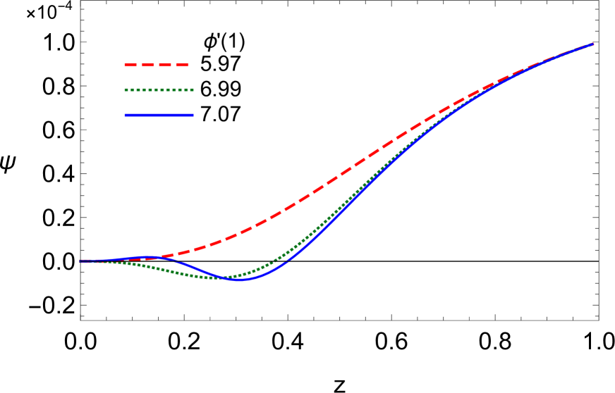
(c)  $\alpha=0.01,b=0.01$

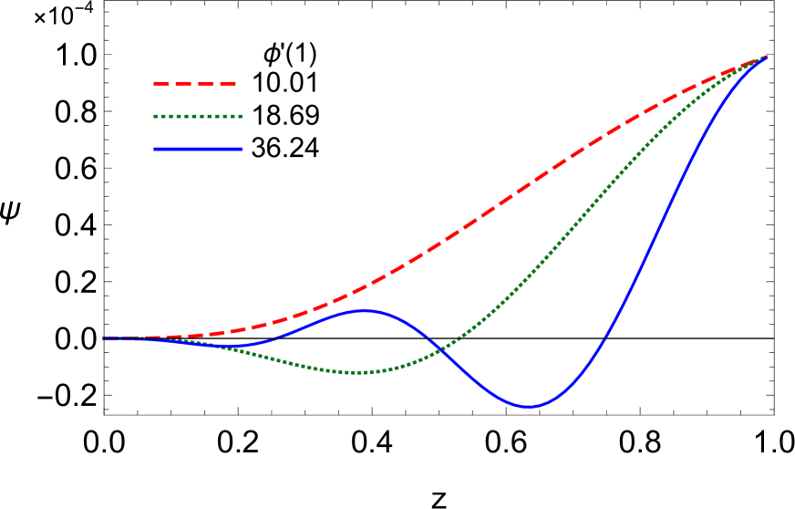
(d)  $\alpha=0.1,b=0$

Figure 1: The behavior of $\psi(z)$ versus $z$ for Gauss-Bonnet HSC and for $\tilde{m}^{2}=-3$ and different $\alpha$ and $b$.

$b$	$a$	$\lambda_{\mathrm{min}}^{2}$	$\zeta_{SL}\left(=\frac{1}{\pi\lambda_{\mathrm{min}}^{1/3}}\right)$	$\zeta_{\mathrm{Numerical}}$
0	0.721772	18.2331	0.196204	0.197957
0.01	0.747560	25.0682	0.186064	0.181057
0.02	0.777479	36.1392	0.175060	0.165642
0.03	0.809805	55.2025	0.163126	0.151671

Table 1: Comparison of analytical and numerical values of $\zeta=T_{c}/\rho^{1/3}$ for $\alpha=0.0001$.

$b$	$a$	$\lambda_{\mathrm{min}}^{2}$	$\zeta_{SL}\left(=\frac{1}{\pi\lambda_{\mathrm{min}}^{1/3}}\right)$	$\zeta_{\mathrm{Numerical}}$
0	0.720561	18.5392	0.195660	0.196843
0.01	0.747087	25.6427	0.185363	0.179433
0.02	0.777900	37.2577	0.174173	0.163592
0.03	0.811046	57.4907	0.162026	0.149279

Table 2: Comparison of analytical and numerical values of $\zeta=T_{c}/\rho^{1/3}$ for $\alpha=0.01$.

$b$	$a$	$\lambda_{\mathrm{min}}^{2}$	$\zeta_{SL}\left(=\frac{1}{\pi\lambda_{\mathrm{min}}^{1/3}}\right)$	$\zeta_{\mathrm{Numerical}}$
0	0.709061	21.5679	0.190787	0.186114
0.01	0.743348	31.6982	0.178928	0.162657
0.02	0.783517	49.9342	0.165876	0.141983
0.03	0.823574	85.6808	0.151601	0.124005

Table 3: Comparison of analytical and numerical values of $\zeta=T_{c}/\rho^{1/3}$ for $\alpha=0.1$.

We calculate $\phi^{{}^{\prime\prime}}(1)$, $\psi^{{}^{\prime}}(1)$ and $\psi^{{}^{\prime\prime}}(1)$ in the term of $\psi(1)$ and $\phi^{{}^{\prime}}(1)$ by using the equations of motion for $\phi$ and $\psi$, namely Eqs. (39) and (40), respectively. Since near the critical point $\psi$ is very small, thus we choose $\psi(1)=0.0001$. Our strategy for using the shooting method is as follows. For specific value of the reduced scalar field mass $\tilde{m}^{2}$, we can perform numerical calculation near the horizon boundary with one shooting parameter $\phi^{{}^{\prime}}(1)$ to get proper solutions at the infinite boundary. For specific values of $\phi^{{}^{\prime}}(1)$, we impose the boundary condition $\psi_{-}=0$. We also calculate the analytical values and numerical values of $\zeta$ for different $b$. We compare our numerical results with analytical in tables $1$, $2$ and $3$.

In Fig. 1, we plot $\psi$ versus $z$ for three first boundary condition $\phi^{{}^{\prime}}(1)$, $\tilde{m}^{2}=-3$ and different values of Gauss-Bonnet coefficient $\alpha$ and nonlinear parameter $b$. In the absence of quadratic correction term ($b=0$), our results exactly coincide with those presented in [17, 20]. The acceptable diagram for us is the red one in each plot since there is nothing in the bulk to effect on speed of the wave, so the diagram of $\psi$ will be stable. From tables $1-3$, it is evident that when $b$ becomes larger the condensation gets harder. Similar behavior can be seen for the fixed value of $b$ and different values of $\alpha$, namely the critical temperature reduces and condensation becomes harder when the Gauss-Bonnet coupling parameter $\alpha$ gets larger.

4 Critical exponent and condensation values

In this section, our aim is to calculate the critical exponent of HSC with first order correction terms in gravity and gauge field. Again, we continue our studying both analytically and numerically.

4.1 Analytical method

We would like to obtain the critical exponent and the condensation values of the condensation operator near the critical temperature using the analytical method. Inserting Eq. (25) into Eq. (20), we get

$$\partial_{z}^{2}\phi-\frac{1}{z}\partial_{z}\phi+\frac{6bz^{3}}{r_{+}^{2}}(\partial_{z}\phi)^{3}=\frac{\langle\mathcal{O_{+}}\rangle^{2}}{r_{+}^{4}}\mathcal{B}\phi,$$ (45)

and,

$$\mathcal{B}=\frac{2z^{2}}{f}\left(1-\frac{3bz^{4}(\partial_{z}\phi)^{2}}{r_{+}^{2}}\right)F^{2}(z).$$ (46)

Near the critical temperature, $\frac{\langle\mathcal{O_{+}}\rangle^{2}}{r_{+}^{4}}$ is a very small and thus we can expand $\phi(z)$ as

$$\frac{\phi(z)}{r_{+}}=\lambda(1-z^{2})\left[1-\frac{b\lambda^{2}}{2}\xi(z)\right]+\frac{\langle\mathcal{O_{+}}\rangle^{2}}{r_{+}^{4}}\chi(z).$$ (47)

where $\chi$ satisfies the following boundary condition

$$\chi(1)=\chi^{{}^{\prime}}(1)=0.$$ (48)

With the help of Eq. (47), and comparing the coefficient of $\frac{\langle\mathcal{O_{+}}\rangle^{2}}{r_{+}^{4}}$ on both sides, Eq. (45) leads to

$$\chi^{{}^{\prime\prime}}(z)-\frac{\chi^{{}^{\prime}}}{z}+72b\lambda^{2}z^{5}\chi^{{}^{\prime}}=\lambda\mathcal{B}(1-z^{2})\left(1-\frac{b}{2}\lambda^{2}\xi(z)\right).$$ (49)

From Eq. (49) we figure out, in the limit $z\rightarrow 0$, the following equation

$$\chi^{{}^{\prime\prime}}(0)=\frac{\chi^{{}^{\prime}}(z)}{z}|_{z\rightarrow 0}.$$ (50)

It is a matter of calculations to shaw that Eq. (49) can be written

$$\frac{d}{dz}\left(e^{12b\lambda^{2}z^{6}}\frac{\chi^{{}^{\prime}}}{z}\right)=\lambda\frac{2z^{3}}{r_{+}^{2}}\frac{e^{12b\lambda^{2}z^{6}}(1-\frac{b}{2}\lambda^{2}\Gamma(z))}{(1+z^{2})(1+\alpha(1-z^{4}))}F^{2}(z),$$ (51)

where $\Gamma(z)=1+z^{2}+z^{4}+25z^{6}$. Integrating both sides of the above equation in the interval $[0,1]$ and using the boundary condition (48), we arrive at

$$\frac{\chi^{{}^{\prime}}}{z}|_{z\rightarrow 0}=-\frac{\lambda}{r_{+}^{2}}\mathcal{A},$$ (52)

where

$$\mathcal{A} \approx \int_{0}^{1}\frac{2z^{3}F^{2}(z)\left[1-\frac{b}{2}\lambda^{2}(1+z^{2}+z^{4}+z^{6})\right][1-\alpha(1-z^{4})]}{1+z^{2}}dz.$$

Combining Eqs. (18) and (47), we achieve

$$\frac{\mu}{r_{+}}-\frac{\rho}{r_{+}^{3}}z^{2}=\lambda(1-z^{2})\left[1-\frac{b\lambda^{2}}{2}\xi(z)\right]+\frac{\langle\mathcal{O_{+}}\rangle^{2}}{r_{+}^{4}}(\chi(0)+z\chi^{{}^{\prime}}(0)+\frac{z^{2}}{2}\chi^{{}^{\prime\prime}}(0)+...),$$ (53)

where in the last step we have expanded $\chi(z)$ around $z=0$. Equating the coefficients of $z^{2}$ on both sides of Eq. (53), we find

$$\frac{\rho}{r_{+}^{3}}=\lambda\left(1+\frac{\langle\mathcal{O_{+}}\rangle^{2}}{r_{+}^{6}}\mathcal{A}\right).$$ (54)

Using the fact that $\lambda={\rho}/{r^{3}_{+c}}$ as well as definition (11), we can obtain the order parameter $\langle\mathcal{O_{+}}\rangle$ near the critical temperature $T_{c}$ as

$$\langle\mathcal{O_{+}}\rangle=\gamma\pi^{3}T_{c}^{3}\sqrt{1-\frac{T}{T_{c}}},$$ (55)

where

$$\gamma=\sqrt{\frac{6}{\mathcal{A}}}.$$ (56)

From Eq. (55) we observe that the critical exponent has the mean field value $1/2$, which is independent of the nonlinear parameter $b$ and Gauss-Bonnet parameter $\alpha$. It is worth noting that $\langle\mathcal{O}\rangle$ is zero at $T=T_{c}$ and condensation occurs for $T<T_{c}$. We shall back to calculation the condensation value $\gamma$ in the next subsection.

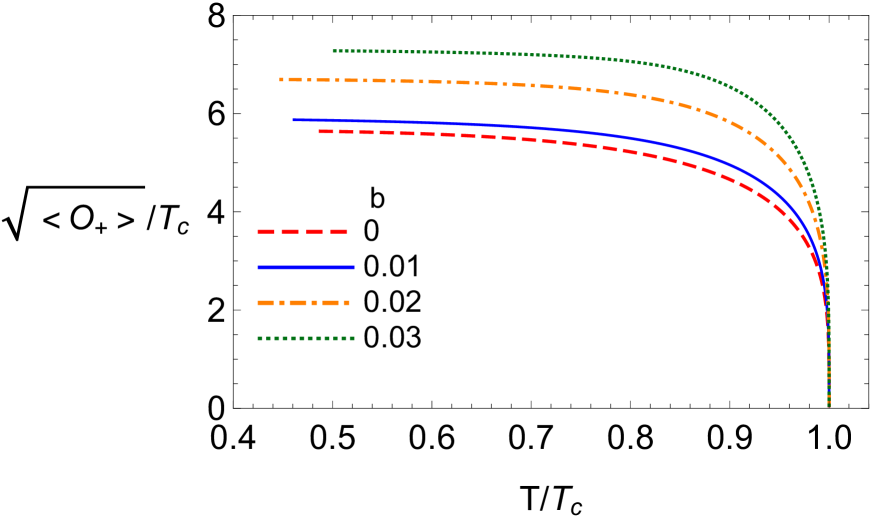
(a)  $\alpha=0.0001$

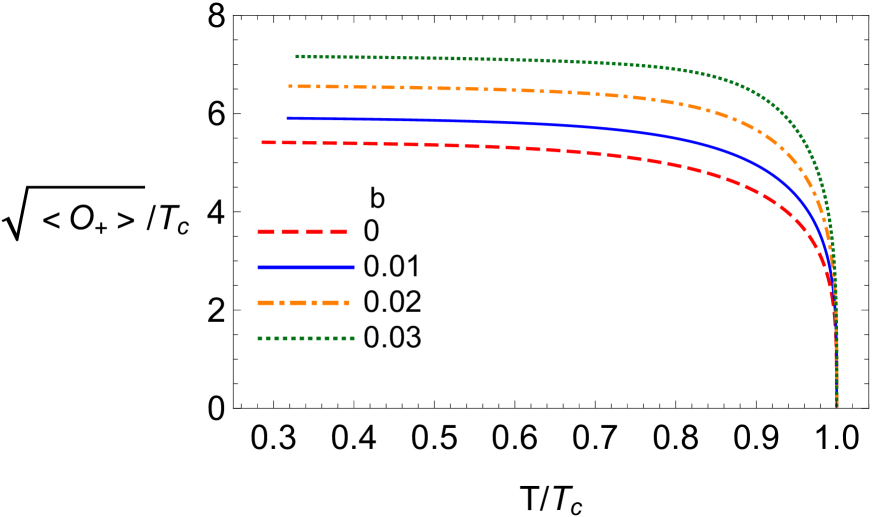
(b)  $\alpha=0.01$

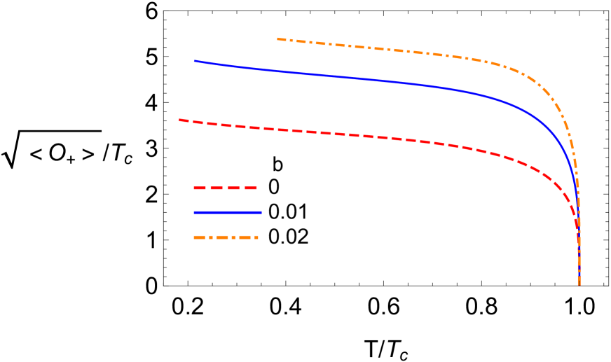
(c)  $\alpha=0.1$

Figure 2: The condensate operator $<\mathcal{O}_{+}>$ as a function of temperature for different values of $b$ and various values of $\alpha$, where we have set $<\mathcal{O}_{-}>=0$ and $\tilde{m}^{2}=-3$.

4.2 Numerical method

We use the numerical method to explore the behaviour of the condensate operator $\langle\mathcal{O}_{+}\rangle$ in terms of temperature for different values of $\alpha$ and $b$ (see Fig. 2). These curves are obtained by the shooting method which we described in the previous section. As one can see from this figure there is a critical temperature $T_{c}$ below which the condensate appears, then rises quickly as the system is cooled and finally goes to a constant for sufficiently low temperatures. This behaviour is qualitatively similar to that obtained in BCS theory and observed in many materials.

$b$	$a$	$\lambda_{\mathrm{min}}^{2}$	$\gamma_{SL}$	$\gamma_{\mathrm{Numerical}}$
0	0.721772	18.2331	7.70525	12.4879
0.01	0.747560	25.0682	9.05565	17.4138
0.02	0.777479	36.1392	14.4103	24.5663

Table 4: The analytical and numerical results for the condensation operator for $\alpha=0.0001.$

$b$	$a$	$\lambda_{\mathrm{min}}^{2}$	$\gamma_{SL}$	$\gamma_{\mathrm{Numerical}}$
0	0.720561	18.5392	7.72419	11.2411
0.01	0.747087	25.6427	9.44846	15.9088
0.02	0.777900	37.2577	15.6715	23.5892

Table 5: The analytical and numerical results for the condensation operator for $\alpha=0.01.$

$b$	$a$	$\lambda_{\mathrm{min}}^{2}$	$\gamma_{SL}$	$\gamma_{\mathrm{Numerical}}$
0	0.709061	21.5679	7.90303	4.05071
0.01	0.743348	31.6982	9.81189	10.0376
0.02	0.783517	49.9342	37.6568	17.7555

Table 6: The analytical and numerical results for the condensation operator for $\alpha=0.1.$

Now we are going to study the condensation operator $\langle\mathcal{O}_{+}\rangle$ in the close neighborhood of the superconductor critical temperature to compute the critical exponents and the condensation value $\gamma$ of the Gauss-Bonnet HSC with quadratic nonlinear electromagnetic. For this purpose, we first take the logarithmic of Eq. (55). We arrive at

$$\mathcal{\log}\left(\frac{\langle\mathcal{O_{+}}\rangle}{T_{c}^{3}}\right)=\mathcal{\log}\left(\pi^{3}\gamma\right)+\frac{1}{2}\mathcal{\log}\left(1-\frac{T}{T_{c}}\right).$$ (57)

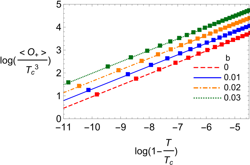
(a)  $\alpha=0.0001$

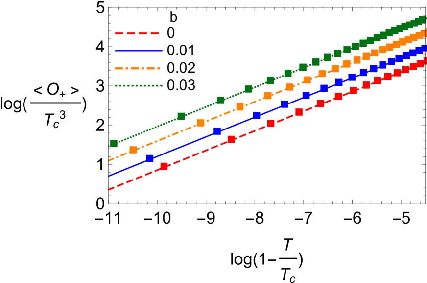
(b)  $\alpha=0.01$

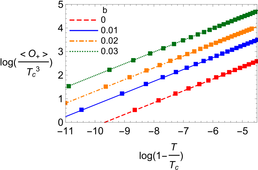
(c)  $\alpha=0.1$

Figure 3: These figures show the behavior of $\log{\left(<\mathcal{O}_{+}>/T_{c}^{3}\right)}$ versus $\log\left(1-T/Tc\right)$ near the critical temperature $Tc$ for different values of $b$ and $\alpha$. The numerical results are highlighted in the filled squares.

We have plotted the behaviour of the above function in Fig. (3). From this figure, we observe that the numerical results are fitted to the above analytic form in the vicinity of the critical temperature. We summarize our results in Fig. (3) and also tables $4-6$ for different values of $b$ and $\alpha$. We see that for a fixed value of $\alpha$, the condensation operator $\gamma$ increases with increasing $b$, while for a fixed value of $b$, it decreases with increasing $\alpha$.

5 Holographic Conductivity

In this section, we study the energy gap in the holographic superconductor phase which is constructed on the boundary of the background spacetime. In particular, we investigate the influence of the Gauss-Bonnet and nonlinear parameters on the superconducting gap. In order to do this, we must compute the electrical conductivity of holographic superconductor by turning on a small perturbation $\delta A_{x}=A_{x}(r)\exp(-i\omega t)$ to the gauge field in the bulk where $\omega$ is the frequency. At linearized order in perturbation ($\delta A_{x}$), the equation of motion for the gauge field $A_{x}(r)$, which obeys Eq. (7), is

$$\partial_{r}^{2}A_{x}+\left[\frac{1}{r}\left(1-6b\partial_{r}\phi^{2}\right)+\frac{\partial_{r}f}{f}+\frac{4b\phi\partial_{r}\phi\psi^{2}}{f}\right]\partial_{r}A_{x}-\left[\frac{2\psi^{2}}{f}\left(1-b\partial_{r}\phi^{2}\right)-\frac{\omega^{2}}{f^{2}}\right]A_{x}=0.$$ (58)

In the absence of the nonlinear correction ($b=0$), this differential equation reduces to the Maxwell case as presented in [2, 3]. To determine the conductivity, we need the asymptotic ($r\rightarrow\infty$) form of the second order differential equation (58), which may be obtained as

$$\partial_{r}^{2}A_{x}+\frac{3}{r}\partial_{r}A_{x}+\frac{\omega^{2}L_{\mathrm{eff}}^{4}}{r^{4}}A_{x}+\ldots=0,$$ (59)

which admits the following solution near the boundary

$$A_{x}=A_{x}^{(0)}+\frac{A_{x}^{(1)}}{r^{2}}+\frac{\omega^{2}L_{\mathrm{eff}}^{4}\mathrm{ln}(Kr)}{2r^{2}}A_{x}^{(0)}+\cdots,$$ (60)

where $A_{x}^{(0)}$, $A_{x}^{(1)}$ are two constant and $K$ is also a constant parameter with length dimension which is considered for a dimensionless logarithmic argument.

According to AdS/CFT correspondence, the two point correlation function of the current operators in a system is given by its on shell action where the action is evaluated on the equations of motion. Here, the on shell action is

$$S_{o.s.}\equiv\int_{r_{+}}^{r_{\infty}}dr\int d^{4}x\sqrt{-g}\mathcal{L},$$ (61)

which, in the quadratic approximation for the gauge field perturbation becomes

$$S_{o.s.}=\int d^{4}x\int_{r_{+}}^{r_{\infty}}dr\Bigg{\{}-\frac{1}{2}r\left[\left(2\psi(r)^{2}-\frac{\omega^{2}}{f(r)}-\frac{b\omega^{2}\partial_{r}\phi^{2}}{f(r)}\right)A_{x}(r)^{2}+f(r)\left(1+b\partial_{r}\phi^{2}\right)\partial_{r}A_{x}(r)^{2}\right]\Bigg{\}}.$$ (62)

After performing an integration by parts and using Eq. (58), we get

$$S_{o.s.}=\int d^{4}x\left[-\frac{1}{2}rf(r)\left(1+b\partial_{r}\phi^{2}\right)\partial_{r}A_{x}(r)A_{x}(r)\right]\Bigg{|}_{r=r_{\infty}}.$$ (63)

Substituting Eqs. (12), (18) and (60) in the above expression, one arrives at

$$S_{o.s.}=\int d^{4}x\left[\frac{A_{x}^{(0)}A_{x}^{(1)}}{L_{\mathrm{eff}}^{2}}-\frac{\omega^{2}L_{\mathrm{eff}}^{2}A_{x}^{(0)2}}{4}+\frac{1}{2}\omega^{2}L_{\mathrm{eff}}^{2}\mathrm{ln}(Kr)A_{x}^{(0)2}+\frac{A_{x}^{(1)2}}{L_{\mathrm{eff}}^{2}r^{2}}\right.$$

$$-\frac{\omega^{2}L_{\mathrm{eff}}^{2}A_{x}^{(0)}A_{x}^{(1)}}{4r^{2}}-\frac{\omega^{2}L_{\mathrm{eff}}^{6}\mathrm{ln}(Kr)A_{x}^{(0)2}}{8r^{2}}+\frac{\omega^{2}L_{\mathrm{eff}}^{2}\mathrm{ln}(Kr)A_{x}^{(0)}A_{x}^{(1)}}{r^{2}}$$

$$\left.+\frac{\omega^{4}L_{\mathrm{eff}}^{6}\mathrm{ln}(Kr)A_{x}^{(0)2}}{4r^{2}}+\mathcal{O}\left(\frac{1}{r^{3}}\right)\right]\Bigg{|}_{r=r_{\infty}},$$ (64)

thus we can obtain $S_{o.s.}$ as follows

$$S_{o.s.}=\int d^{4}x\left[\frac{A_{x}^{(0)}A_{x}^{(1)}}{L_{\mathrm{eff}}^{2}}-\frac{\omega^{2}L_{\mathrm{eff}}^{2}A_{x}^{(0)2}}{4}+\frac{1}{2}\omega^{2}L_{\mathrm{eff}}^{2}\mathrm{ln}(Kr)A_{x}^{(0)2}\right],$$ (65)

in which logarithmic divergences appears. In order to cancel out this divergency, we obtain the boundary counterterm as described in Appendix by using Skenderis’s method of holographic renormalization [68]. Therefore, the finite on shell action may be written as

$$S=S_{o.s.}+S_{c.t.},$$ (66)

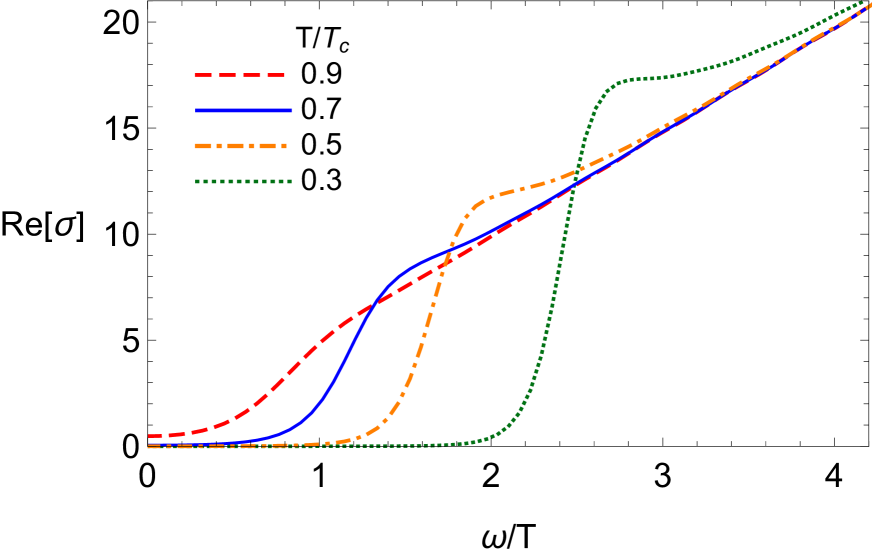
(a)  $\alpha=0.0001,b=0$

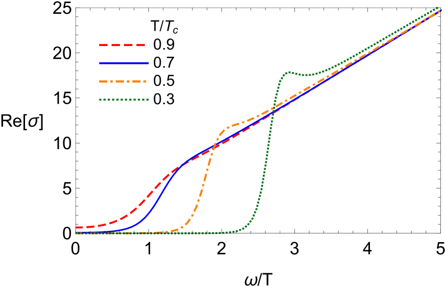
(b)  $\alpha=0.0001,b=0.01$

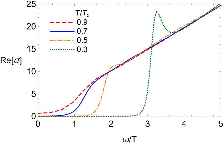
(c)  $\alpha=0.0001,b=0.02$

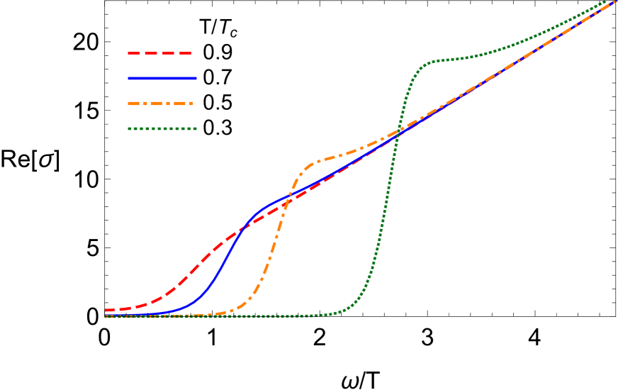
(d)  $\alpha=0.01,b=0$

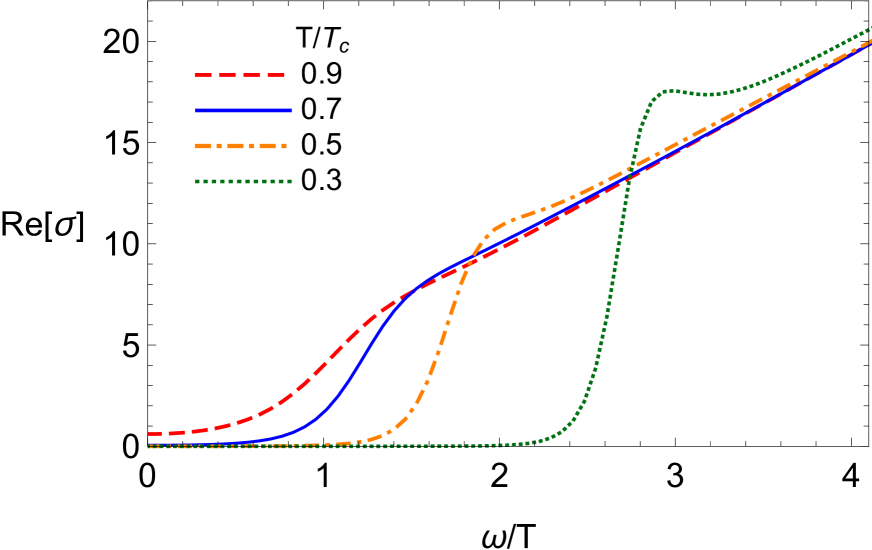
(e)  $\alpha=0.01,b=0.01$

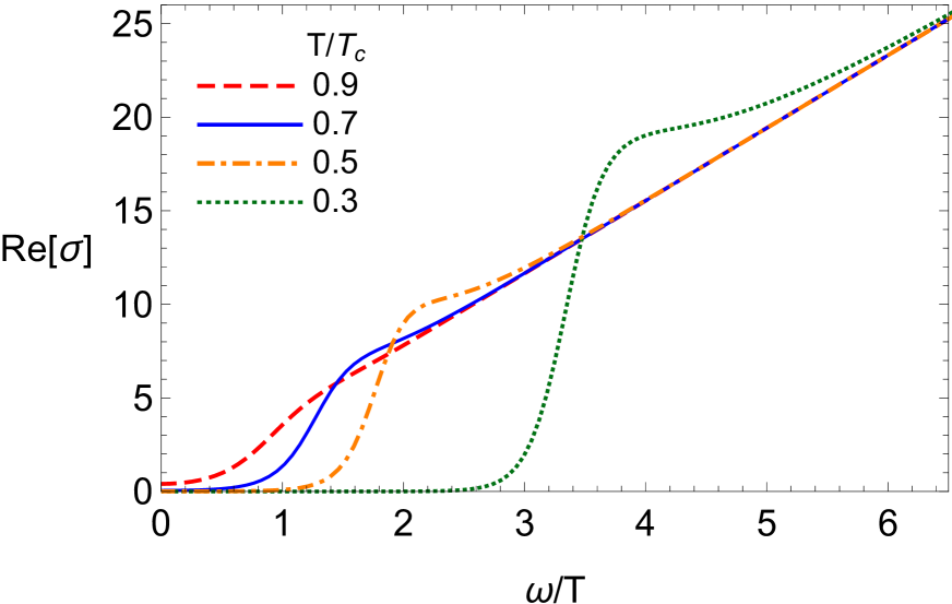
(f)  $\alpha=0.1,b=0$

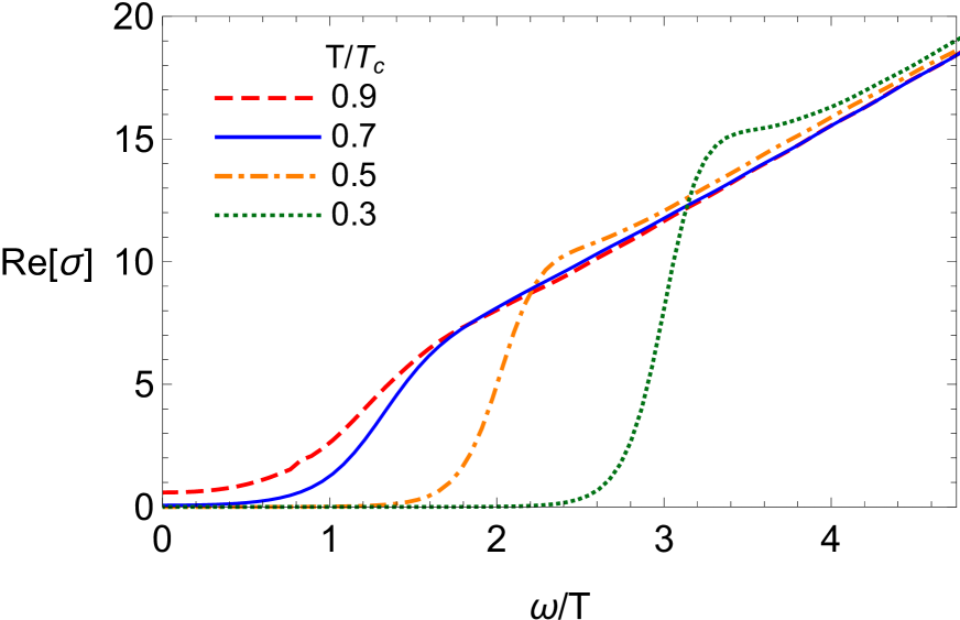
(g)  $\alpha=0.1,b=0.01$

Figure 4: The real part of the conductivity as a function of frequency for different values of $b$ and $\alpha$. Each figure is plotted for different temperature $T/Tc$.

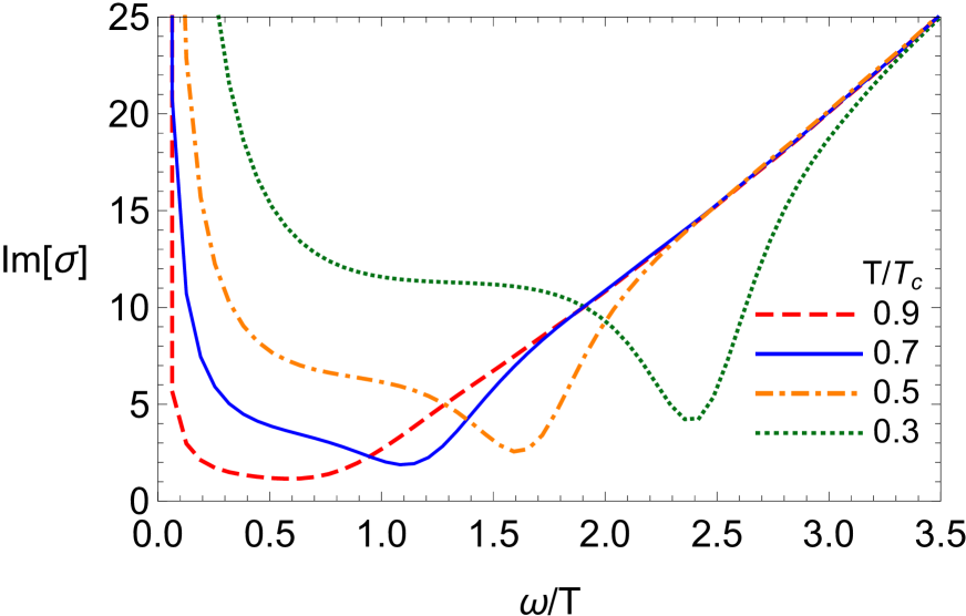
(a)  $\alpha=0.0001,b=0$

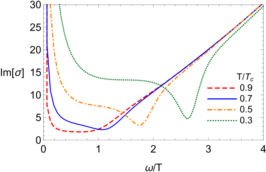
(b)  $\alpha=0.0001,b=0.01$

(c)  $\alpha=0.0001,b=0.02$

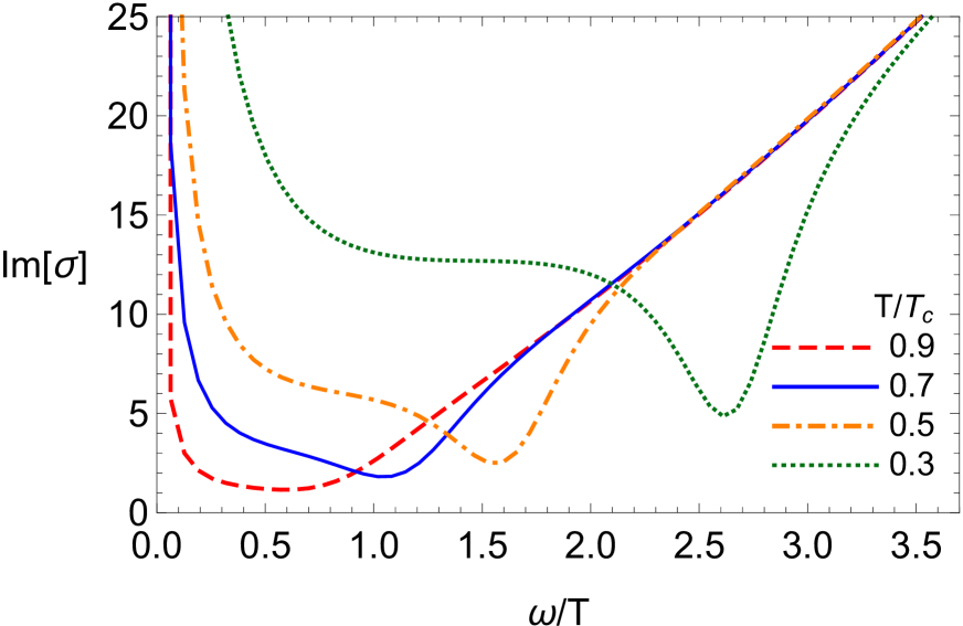
(d)  $\alpha=0.01,b=0$

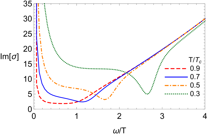
(e)  $\alpha=0.01,b=0.01$

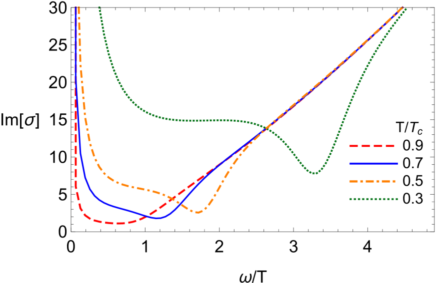
(f)  $\alpha=0.1,b=0$

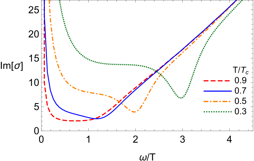
(g)  $\alpha=0.1,b=0.01$

Figure 5: The imaginary part of the conductivity as a function of frequency for different values of $b$ and $\alpha$. Each figure is plotted for different temperature $T/Tc$.

where the gauge invariant counterterm $S_{c.t.}$ is given by Eq. (79). Now, we can obtain the current operator in the boundary field theory [2, 3] as

$$\left\langle J_{x}\right\rangle=\frac{\delta S}{\delta A_{x}^{(0)}}=\frac{2}{L_{\mathrm{eff}}^{2}}A_{x}^{(1)}-\frac{\omega^{2}L_{\mathrm{eff}}^{2}}{2}A_{x}^{(0)}\text{ }.$$ (67)

According to Ohm’s law, the electrical conductivity can be expressed as

$$\sigma\left(\omega\right)=\frac{\left\langle J_{x}\right\rangle}{E_{x}},$$ (68)

where $E_{x}=-\partial_{t}\delta A_{x}$. Hence, using the current (67), the holographic conductivity is given by

$$\sigma=-\frac{2iA_{x}^{(1)}}{\omega L_{\mathrm{eff}}^{2}A_{x}^{(0)}}+\frac{i\omega L_{\mathrm{eff}}^{2}}{2}.$$ (69)

Consequently, the holography conductivity is calculated by solving numerically a differential equation (58) such that the infalling boundary condition is imposed at the event horizon

$$A_{x}(r)=\mathrm{exp}\left(-\frac{i\omega}{4\pi T}\right)S(r),$$ (70)

in which $T$ is the Hawking temperature and

$$S(r)=1+a_{1}(r-r_{+})+a_{2}(r-r_{+})^{2}+\ldots,$$ (71)

where $a_{1},a_{2},\ldots$ are calculated by Taylor series expansion of equation (58) around the horizon.

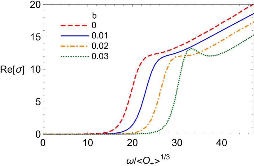
(a)  $\alpha=0.0001$

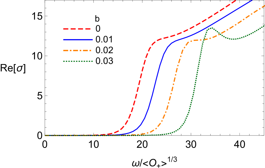
(b)  $\alpha=0.01$

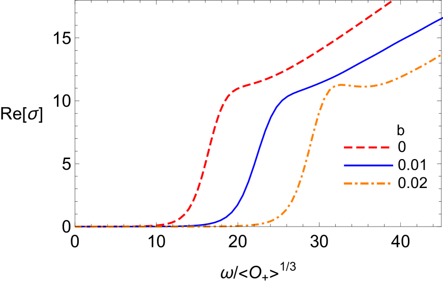
(c)  $\alpha=0.1$

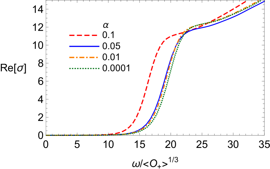
(d)  $b=0$

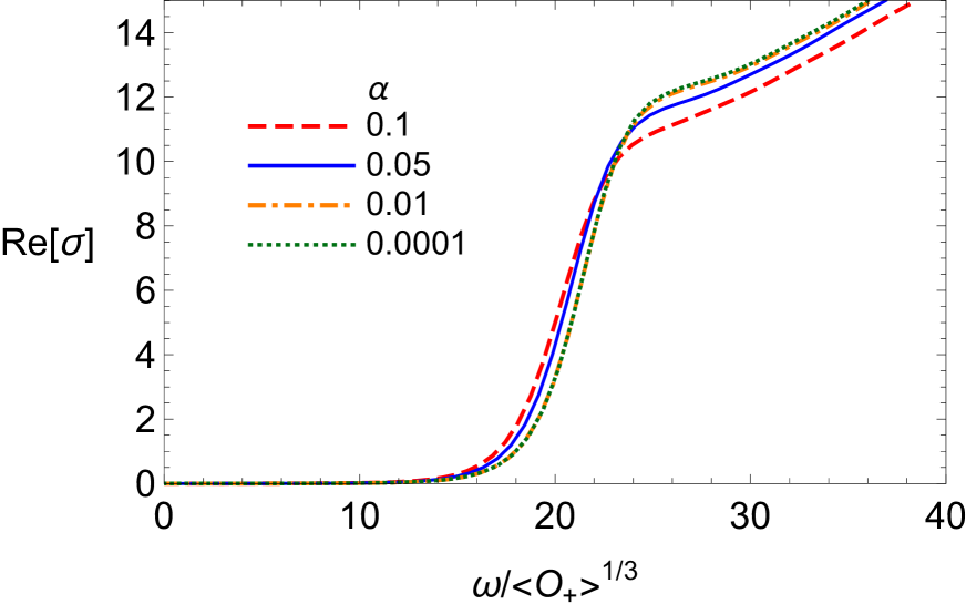
(e)  $b=0.005$

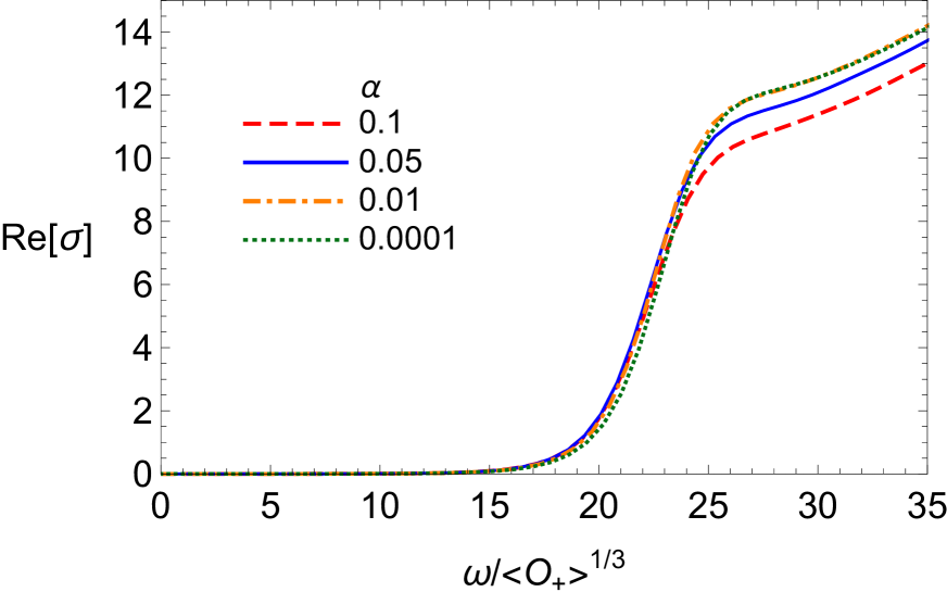
(f)  $b=0.01$

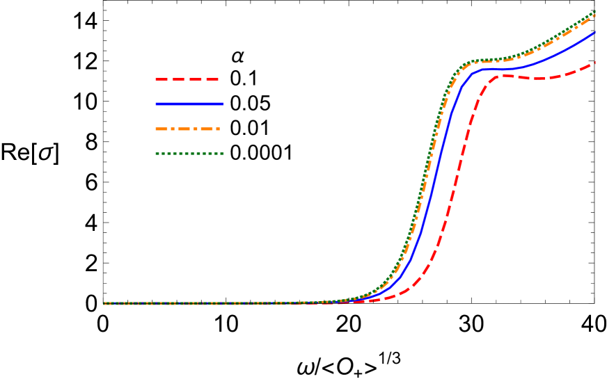
(g)  $b=0.02$

Figure 6: The real part of the conductivity as a function of $\omega/<\mathcal{O_{+}}>^{1/3}$, at low temperatures, around $T\approx 0.1Tc$.

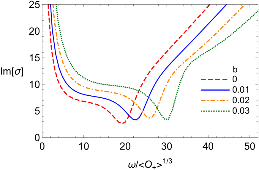
(a)  $\alpha=0.0001$

(b) $\alpha=0.01$

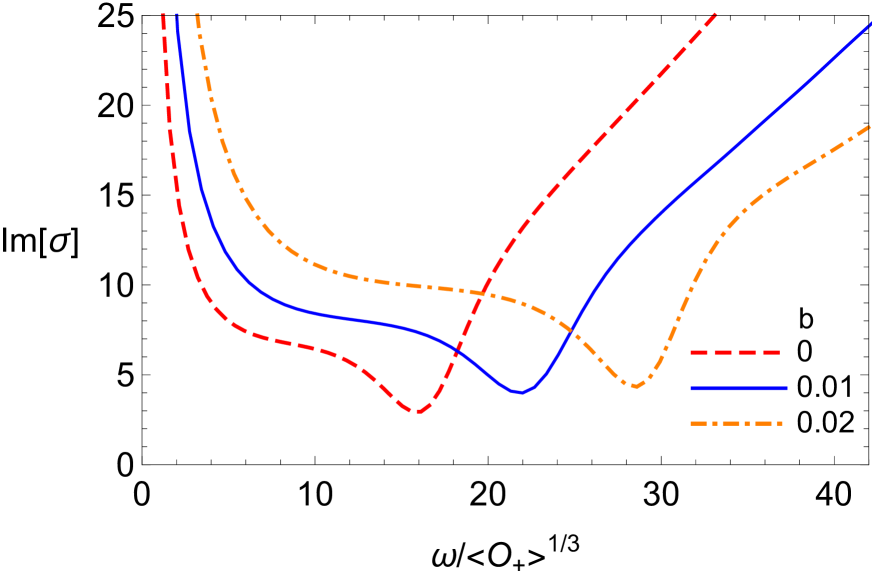
(c)  $\alpha=0.1$

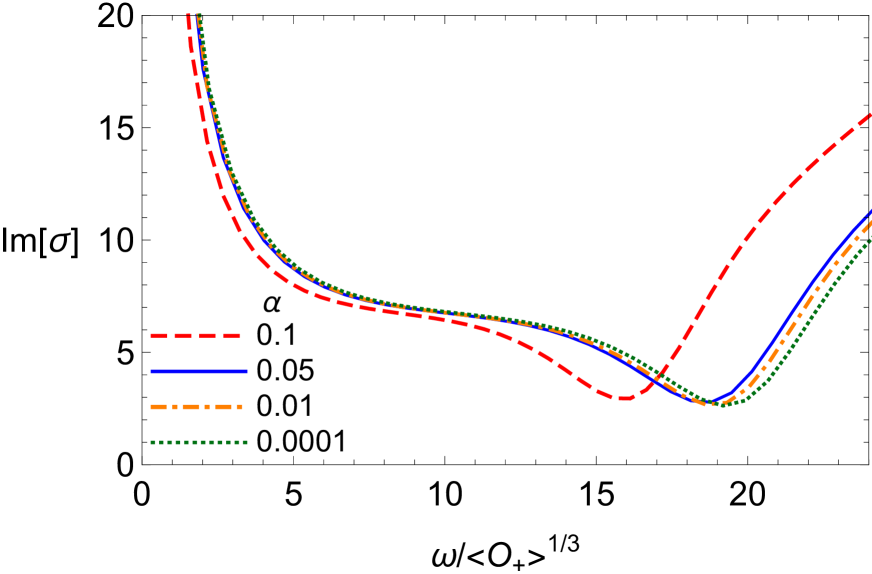
(d)  $b=0$

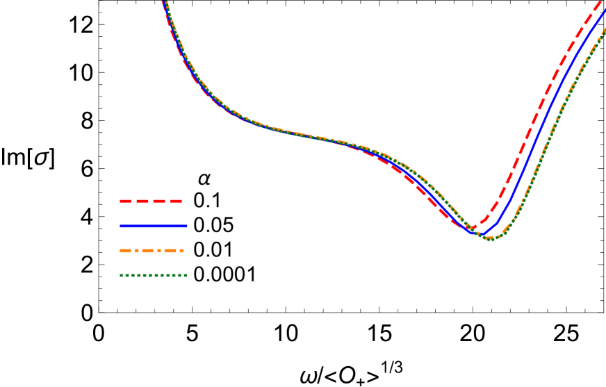
(e)  $b=0.005$

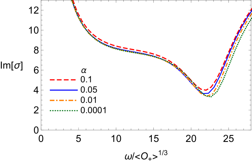
(f)  $b=0.01$

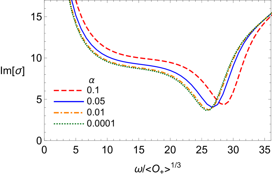
(g)  $b=0.02$

Figure 7: The imaginary part of the conductivity as a function of $\omega/<\mathcal{O_{+}}>^{1/3}$, at low temperatures, around $T\approx 0.1Tc$.

The numerical results for holographic conductivity associated with the condensation operator $<\mathcal{O_{+}}>$ are plotted in Figs. 4-7. The real and imaginary parts of electrical conductivity versus frequency are illustrated at different temperature below $Tc$ in Figs.4 and 5, respectively. As one can see from Fig. 4, the superconducting gap is opened below the critical temperature which became deeper with decreasing the temperature. Besides, for various values of $\alpha$ and $b$, the real part of conductivity is proportional to the frequency per temperature, $\omega/T$, as frequency is enough large. According to the Fig. 5 the divergence in imaginary part, at $\omega=0$, points out a delta function in the real part, $Re[\sigma]$, at $\omega=0$ which is not played in the Fig. 4. As one can see from Fig. 5, the holographic conductivity of HSC has a minimum in the imaginary part. Thus with decreasing the temperature the minimum in the imaginary part shifts toward greater frequency for various values of the Gauss-Bonnet and nonlinear parameters.

To study formation of the superconducting gap with changing $\alpha$ and $b$ at low temperature, e.g., $T\approx 0.1Tc$, the real and imaginary parts of holographic conductivity as a function of $\omega/{<\mathcal{O_{+}}>}^{1/3}$ are plotted in Figs. 6 and 7, respectively. For a fixed value of Gauss-Bonnet coefficient $\alpha$, the energy gap ($\omega/{<\mathcal{O_{+}}>}^{1/3}$) enlarges with increasing the nonlinear parameter $b$. It is evident from Figs. 6 and 7, that the energy gap of HSC for various $\alpha$ exhibits different behavior based on the nonlinear correction $b$. In case of the Maxwell field ($b=0$), the superconducting energy gap decreases as $\alpha$ increases at low temperature (see Fig. 6(d)). When we take into account the nonlinear correction $b$, the energy gap of HSC increases with increasing $\alpha$ (see Figs. 6(d)-6(g)). From Fig. 7, we see that for a fixed value of $\alpha$, the minimum of imaginary part of conductivity goes to the larger value of $\omega/<\mathcal{O_{+}}>^{1/3}$ when $b$ increases. In the absence of correction ($b=0$), it decreases with enhancing the Gauss-Bonnet coefficient (Fig. 6(d)). Besides, for a fixed value of $b$, the minimum of $\mathrm{Im[\sigma]}$ increases with increasing $\alpha$, while for a fixed value of $\alpha$, it increase with increasing $b$.

6 Conclusions

In this paper, we continue the studies on the $s$-wave holographic superconductors (HSC) by taking into account the higher correction terms both to the gravity side as well as the gauge field side of the system. We considered the Gauss-Bonnet HSC when the Maxwell Lagrangian has a nonlinear correction term and is written in the form $\mathcal{L}=\mathcal{F}+b\mathcal{F}^{2}$, where $\mathcal{F}$ is the Maxwell lagrangian. We have provided several motivations for choosing this kind of Lagrangian for the gauge field. For example, all well-known nonlinear Lagrangian has a series expansion which their first two terms are exactly in the above form.

First, we have analytically as well as numerically investigated the relation between critical temperature of phase transition and charge density which depends on both the Gauss-Bonnet parameter $\alpha$ and the nonlinear parameter $b$. For this purpose, we employed the analytical Sturm-Liouville eigenvalue problem and the numerical shooting method. We find out that for a fixed value of $\alpha$, with increasing the nonlinear parameter $b$, the value of $T_{c}/\rho^{1/3}$ decreases as well. This implies that when $b$ becomes larger the condensation gets harder. Similar behavior can be seen for the fixed value of $b$ and different values of $\alpha$, namely the critical temperature decreases and the condensation becomes harder when the Gauss-Bonnet coupling parameter $\alpha$ gets larger. We confirmed that this results are in a very good agreement with our numerical results. Then, we obtained the critical exponent of the Gauss-Bonnet HSC with nonlinear gauge field. We observed that the critical exponent has the mean field value $1/2$, which is independent of the nonlinear parameter $b$ and Gauss-Bonnet parameter $\alpha$.

Then, we explored, numerically, the holographic conductivity of the system. For this purpose, we plotted the real and imaginary parts of electrical conductivity versus $\omega/T$ and $\omega/<\mathcal{O_{+}}>^{1/3}$ for $T<Tc$. We observed that the superconducting gap is opened below the critical temperature which became deeper with decreasing the temperature. Interstingly enough, we found that for different values of $\alpha$ and $b$, and for large frequency, the real part of conductivity is proportional to $\omega/T$. We observed that the holographic conductivity of HSC has a minimum in the imaginary part. Besides, with decreasing the temperature the minimum in the imaginary part shifts toward greater frequency for various values of the Gauss-Bonnet parameter $\alpha$ and nonlinear gauge field parameter $b$. Furthermore, for a fixed value of $b$, the minimum of $\mathrm{Im[\sigma]}$ increases with increasing $\alpha$, while for a fixed value of $\alpha$, it increase with increasing $b$.

Appendix: Holographic renormalization

To construct the boundary counterterm action, we utilize a holographic renormalization method of Skenderis which was presented in [68, 69, 70]. To apply this method, the spacetime metric takes the form

$$ds^{2}=G_{ab}d\xi^{a}d\xi^{b}=-\frac{L_{\mathrm{eff}}^{2}}{\varrho}\mathcal{X}(\varrho)d\tau^{2}+\frac{L_{\mathrm{eff}}^{2}d\varrho^{2}}{4\varrho\mathcal{X}(\varrho)}+\frac{L_{\mathrm{eff}}^{2}}{\varrho}(dx^{2}+dy^{2}+dz^{2}),$$ (72)

which relates to the metric (9) via $\tau=t/L_{\mathrm{eff}}$, $\varrho=L_{\mathrm{eff}}^{2}/r$ and the asymptotic ($\varrho\rightarrow 0$) metric function is $\mathcal{X}(\varrho)_{\varrho\rightarrow 0}=1$. Hence, asymptotically metric becomes

$$ds^{2}=\frac{L_{\mathrm{eff}}^{2}d\varrho^{2}}{4\varrho\mathcal{X}(\varrho)}+h_{\mu\nu}dx^{\mu}dx^{\nu},$$ (73)

where

$$h_{\mu\nu}=\frac{L_{\mathrm{eff}}^{2}}{\varrho}\gamma_{\mu\nu}^{0}.$$ (74)

According to the electromagnetic contribution, one can evaluate the on-shell action as

$$S = \int_{\mathcal{M}}d^{5}\xi\sqrt{-G}\left[\mathcal{F}+b\mathcal{F}^{2}\right]$$ (75)

$$= \int_{\mathcal{M}}d^{5}\xi\frac{\sqrt{-G}}{2}A_{b}\nabla_{a}\left[\left(1+2b\mathcal{F}\right)F^{ab}\right]-\int_{\partial\mathcal{M}}d^{4}x\frac{\sqrt{-h}}{2}A_{\mu}F^{\varrho\mu}\left(1+2b\mathcal{F}\right)$$

$$= -L_{\mathrm{eff}}\int_{\varrho=\epsilon}d^{4}x\sqrt{-\gamma^{0}}A_{\mu}\partial_{\varrho}A_{\nu}\gamma^{0\mu\nu}\left(1+2b\mathcal{F}\right),$$

where $\epsilon$ is a small constant parameter. On the new coordinates (72), the gauge field equation of bulk motion near boundary is given by

$$\varrho\frac{d^{2}A_{i}}{d\varrho^{2}}+\frac{1}{4}\partial_{0}^{2}A_{i}+\mathcal{O}(\varrho^{2})=0,$$ (76)

where $\partial_{0}^{2}$ points out to the wave operator of boundary metric $\gamma_{\mu\nu}^{0}$ and the general solution of this equation is

$$A_{i}=A_{i}^{0}+A_{i}^{1}\varrho+\psi\varrho\mathrm{ln}(\varrho),$$ (77)

where $\psi=-1/4\partial_{0}^{2}A_{i}^{0}$. With $A_{i}$ at hand, the on-shell electromagnetic action can be written as

$$S=-L_{\mathrm{eff}}\int_{\varrho=\epsilon}d^{4}x\sqrt{-\gamma^{0}}A_{i}^{0}\left(A_{i}^{1}-\frac{1}{4}\partial_{0}^{2}A_{i}^{0}-\frac{1}{4}\mathrm{ln}(\epsilon)\partial_{0}^{2}A_{i}^{0}\right),$$ (78)

which is logarithmically divergent. Now, according to Ref.[68], in order to determine the counterterm action, we first invert the solution (77) to give $A_{i}^{0}=A_{i}+\mathcal{O}(\epsilon)$. Thus, the counterterm action is obtained as

$$S_{c.t.} = -\frac{L_{\mathrm{eff}}}{4}\mathrm{ln}(\epsilon)\int_{\varrho=\epsilon}d^{4}x\sqrt{-\gamma^{0}}A_{i}\partial_{0}^{2}A_{i}$$ (79)

$$= -\frac{L_{\mathrm{eff}}}{4}\mathrm{ln}(\epsilon)\int_{\varrho=\epsilon}d^{4}x\frac{\sqrt{-h}}{2}F_{\mu\nu}F^{\mu\nu}.$$

It is notable to mention that since we consider $A_{i}=A_{i}(\varrho)\exp(-i\omega L_{\mathrm{eff}}\tau)$, one can calculate

$$\partial_{0}^{2}A_{i}=\omega^{2}L_{\mathrm{eff}}^{2}A_{i}.$$ (80)

References

-
[1]
J. Maldacena, The large N limit of superconformal
field theories and supergravity, Adv. Theor. Math. Phys. 2, 231
(1998), [arXiv:9711200];
S.S. Gubser, I.R. Klebanov, and A.M. Polyakov, Gauge theory correlators from non-Critical string theory, Phys. Lett. B 428, 105 (1998), [arXiv:9802109];
E. Witten, Anti de sitter space and holography, Adv. Theor. Math. Phys. 2, 253 (1998), [arXiv:9802150]. - [2] S. A. Hartnoll, C.P. Herzog and G.T. Horowitz, Building a holographic superconductor, Phys. Rev. Lett. 101, 031601 (2008), [arXiv:0803.3295].
- [3] G.T. Horowitz and M.M. Roberts, Holographic superconductors with various condensates, Phys. Rev. D 78, 126008 (2008), [arXiv:0810.1563].
- [4] S. A. Hartnoll, C. P. Herzog and G. T. Horowitz, Holographic superconductors, JHEP 12, 015 (2008), [arXiv:0810.1563].
- [5] G. T. Horowitz, Introduction to holographic superconductors, Lect. Notes Phys. 828 313 (2011) [arXiv:1002.1722].
- [6] S.S. Gubser, Breaking an Abelian gauge symmetry near a black hole horizon, Phys. Rev. D 78, 065034 (2008), [arXiv:0801.2977].
- [7] D. Musso, Introductory notes on holographic superconductors, [arXiv:1401.1504].
- [8] R. G. Cai, L. Li, Li-Fang Li, Run-Qiu Yang, Introduction to holographic superconductor models, Sci China Phys. Mech. Astron. 58, 060401 (2015), [arXiv:1502.00437].
- [9] X. H. Ge, B. Wang, S. F. Wu, and G. H. Yang, Analytical study on holographic superconductors in external magnetic field, JHEP 08, 108 (2010), [arXiv:1002.4901].
- [10] R. Banerjee, S. Gangopadhyay, D. Roychowdhury, and A. Lala, Holographic s-wave condensate with non-linear electrodynamics: A nontrivial boundary value problem, Phys. Rev. D 87, 104001 (2013), [arXiv:1208.5902v3].
- [11] D. Momeni, M. Raza, and R. Myrzakulov, More on superconductors via gauge/gravity duality with nonlinear Maxwell field, Journal of Gravity, 2013, Article ID 782512.
- [12] C. M. Chen and M. F. Wu, An analytic analysis of phase transitions in holographic superconductors, Prog. Theor. Phys. 126, 387 (2011), [arXiv:1103.5130].
- [13] H. B. Zeng, X. Gao, Y. Jiang, and H. S. Zong, Analytical computation of critical exponents in several holographic superconductors, JHEP 1105, 002 (2011), [arXiv:1012.5564].
- [14] R. G. Cai, H. F Li, H.Q. Zhang, Analytical studies on holographic insulator/superconductor phase transitions, Phys. Rev. D 83, 126007 (2011), [arXiv:1103.5568].
- [15] Q. Pan, B. Wang, E. Papantonopoulos, J. Oliveira, A. B. Pavan, Holographic superconductors with various condensates in Einstein-Gauss-Bonnet gravity, Phys. Rev. D 81, 106007 (2010), [arXiv:0912.2475].
- [16] Q. Pan, B. Wang, General holographic superconductor models with Gauss-Bonnet corrections, Phys. Lett. B 693 159 (2010), [arXiv:1005.4743].
- [17] H. F. Li, R. G. Cai, H. Q. Zhang, Analytical studies on holographic superconductors in Gauss-Bonnet gravity, JHEP 04, 028 (2011), [arXiv:1103.2833].
- [18] L. Barclay, R. Gregory, S. Kanno, P. Sutcliffe, Gauss-Bonnet holographic superconductors, JHEP 1012, 029 (2010), [arXiv:1009.1991].
-
[19]
R. G. Cai, Z.Y. Nie, H.Q. Zhang, Holographic p-wave
superconductors from Gauss-Bonnet gravity, Phys. Rev. D 82, 066007
(2010), [arXiv:1007.3321];
R. G. Cai, Z. Y. Nie, H.Q. Zhang, Holographic Phase Transitions of P-wave Superconductors in Gauss-Bonnet Gravity with Back-reaction, Phys. Rev. D 83, 066013 (2011) [ arXiv:1012.5559];
Q. Pan, J. Jing, B. Wang, Analytical investigation of the phase transition between holographic insulator and superconductor in Gauss-Bonnet gravity, JHEP 11, 088 (2011), [arXiv:1105.6153]. - [20] R. Gregory, S. Kanno and J. Soda, Holographic superconductors with higher curvature corrections, JHEP 0910, 010 (2009) [arXiv:0907.3203].
- [21] R. G. Cai, Z.Y. Nie, H.Q. Zhang, Holographic p-wave superconductors from Gauss-Bonnet gravity, Phys. Rev. D 82, 066007 (2010) [arXiv:1007.3321].
- [22] R. G. Cai, H. F. Li, H. Q. Zhang, Analytical studies on holographic insulator/superconductor phase transitions, Phys. Rev. D 83, 126007 (2011) [arXiv:1103.5568].
- [23] R. G. Cai, L. Li, L. F. Li, A holographic p-wave superconductor model, JHEP 1401, 032 (2014) [arxiv:1309.4877].
- [24] X. H. Ge, S. F. Tu, B. Wang, d-Wave holographic superconductors with backreaction in external magnetic fields, JHEP 09, 088 (2012) [arXiv:1209.4272].
- [25] X. M. Kuang, E. Papantonopoulos, G. Siopsis, B. Wang, Building a Holographic Superconductor with Higher-derivative Couplings, Phys. Rev. D 88, 086008 (2013) [arXiv:1303.2575].
- [26] Q. Pan, J. Jing, B. Wang, S. Chen, Analytical study on holographic superconductors with backreactions, JHEP 06, 087 (2012) [arXiv:1205.3543].
- [27] Q. Pan, J. Jing, B. Wang, Analytical investigation of the phase transition between holographic insulator and superconductor in Gauss-Bonnet gravity, JHEP 11, 088 (2011) [arXiv:1105.6153].
- [28] M. Kord Zangeneh, Y. C. Ong, B. Wang, Entanglement Entropy and Complexity for One-Dimensional Holographic Superconductors , Phys. Lett. B 771, 235 (2017) [arXiv:1704.00557].
- [29] W. Yao, J. Jing, Analytical study on holographic superconductors for Born-Infeld electrodynamics in Gauss-Bonnet gravity with backreactions, JHEP 05, 101 (2013), [arXiv:1306.0064].
- [30] J. Jing, L. Wang, Q. Pan, S. Chen, Holographic Superconductors in Gauss-Bonnet gravity with Born-Infeld electrodynamics, Phys. Rev. D 83, 066010 (2011), [arXiv:1012.0644].
- [31] J. Jing, Q. Pan, S. Chen, Holographic Superconductor/Insulator Transition with logarithmic electromagnetic field in Gauss-Bonnet gravity, Phys. Lett. B 716, 385 (2012) [ arXiv:1209.0893].
- [32] S. Chen, Q. Pan, J. Jing, Holographic superconductors in quintessence AdS black hole, Class. Quantum Grav. 30, 145001 (2013) [arXiv:1206.2069].
- [33] S. Gangopadhyay and D. Roychowdhury, Analytic study of properties of holographic p-wave superconductors, JHEP 08, 104 (2012) [arXiv:1207.5605].
- [34] A. Sheykhi, H. R. Salahi, A. Montakhab, Analytical and Numerical Study of Gauss-Bonnet Holographic Superconductors with Power-Maxwell Field, JHEP 04, 058 (2016) [arXiv:1603.00075].
- [35] H. R. Salahi, A. Sheykhi, A. Montakhab, Effects of Backreaction on Power-Maxwell Holographic Superconductors in Gauss-Bonnet Gravity Eur. Phys. J. C 76 (2016) 575 [arXiv:1608.05025].
- [36] A. Sheykhi, F. Shaker, Analytical study of properties of holographic superconductors with exponential nonlinear electrodynamics, Canadian J. of Phys. 94, (12) (2016) 1372 [arXiv:1601.05817].
- [37] A. Sheykhi, F. Shamsi, Holographic Superconductors with Logarithmic Nonlinear Electrodynamics in an External Magnetic Field, Int. J. Theor. Phys. 56, 916 (2017) [arXiv:1603.02678].
- [38] A. Sheykhi, F. Shamsi, S. Davatolhagh, The upper critical magnetic field of holographic superconductor with conformally invariant Power–Maxwell electrodynamics, Can. J. Phys. 95, 450 (2017) [arXiv:1609.05040].
- [39] R.A. Konoplya and A. Zhidenko, Holographic conductivity of zero temperature superconductors, Phys. Lett. B 686, 199 (2010), [arXiv:0909.2138].
- [40] X.M. Kuang, W.J. Li, and Y. Ling, Holographic Superconductors in Quasi-topological Gravity, JHEP 12, 69 (2010), [arXiv:1008.4066].
- [41] M.R. Setare, D. Momeni, and N. Majd, Holographic superconductors in a model of non-relativistic gravity, JHEP 5, 118 (2011), [arXiv:1003.0376].
- [42] J.P. Wu, Y. Cao, X.M. Kuang, and W.J. Li, The (3+1)-holographic superconductor with Weyl corrections, Phys. Lett. B 697, 153 (2011), [arXiv:1010.1929].
- [43] M.R. Setare and D. Momeni, Gauss-Bonnet holographic superconductors with magnetic field, Euro. Phys. Lett. 96, 60006 (2011), [arXiv:1106.1025].
- [44] D.. Ma, Y. Cao, and J.P. Wu, The Stuckelberg Holographic Superconductors with Weyl corrections, Phys. Lett. B 704, 604 (2011), [arXiv:1201.2486].
- [45] J.P. Wu and P. Liu, Holographic superconductivity from higher derivative theory, Phys. Lett. B 774, 527 (2017), [arXiv:1710.07971].
- [46] A. Dehyadegari, A. Sheykhi and M.K. Zangeneh, Holographic conductivity for logarithmic charged dilaton-Lifshitz solutions, Phys. Lett. B 758, 226 (2016), [arXiv:1602.08476].
- [47] A. Dehyadegari, M. Kord Zangeneh and A. Sheykhi, Holographic conductivity in the massive gravity with power-law Maxwell field,Phys. Lett. B 773, 344 (2017) [arXiv:1703.00975].
- [48] M. Kord Zangeneh, S. S. Hashemi, A. Dehyadegari, A. Sheykhi, B. Wang, Optical properties of Born-Infeld-dilaton-Lifshitz holographic superconductors, [arXiv:1710.10162].
- [49] S. A. Hosseini Mansoori, B. Mirza, A. Mokhtari, F. Lalehgani Dezaki, Z. Sherkatghanad, Weyl holographic superconductor in the Lifshitz black hole background, JHEP 1607, 111 (2016), [arXiv:1602.07245].
- [50] P. Chaturvedi and G. Sengupta, Rotating BTZ Black Holes and One Dimensional Holographic Superconductors, Phys. Rev. D 90, 046002 (2014), [arXiv:1310.5128].
- [51] D. Ghorai and S. Gangopadhyay, Conductivity of holographic superconductors in Born-Infeld electrodynamics, [arXiv:1710.09630].
- [52] K. Lin, E. Abdalla, A. Wang, Holographic superconductors in Horava-Lifshitz gravity, Int. J. Mod. Phys. D 24, 1550038 (2015) [arXiv:1406.4721].
- [53] C. -J. Luo, X.-M. Kuang, F.-W. Shu, Lifshitz holographic superconductor in Horava-Lifshitz gravity, Phys. Lett. B 759, 184 (2016), [arXiv:1605.03260].
- [54] D. Lovelock, J. Math. Phys. 12, 498 (1971).
- [55] B. Zwiebach, Phys. Lett. B 156, 315 (1985).
- [56] S. Gangopadhyay and D. Roychowdhury, Analytic study of properties of holographic superconductors in Born-Infeld electrodynamics, JHEP 5, 2 (2012), [arXiv:1201.6520].
- [57] S. H. Hendi and S. Panahiyan, Thermodynamic instability of topological black holes in Gauss-Bonnet gravity with a generalized electrodynamics, Phys. Rev. D 90, 124008 (2014) [arXiv:1501.05481 [gr-qc]].
- [58] S.H. Hendi, S. Panahiyan and M. Momennia, Extended phase space of AdS Black Holes in Einstein-Gauss-Bonnet gravity with a quadratic nonlinear electrodynamics, Int. J. Mod. Phys. D 25, 1650063 (2016), [arXiv:1503.03340].
- [59] S. H. Hendi, Asymptotic charged BTZ black hole solutions, JHEP 03, 065, (2012)
- [60] A. Ritz and R. Delbourgo, The low-energy effective Lagrangian for photon interactions in any dimension, Int. J. Mod. Phys. A 11, (1996) 253 [hep-th/9503160].
- [61] J.T. Liu and P. Szepietowski, Higher derivative corrections to R-charged AdS5 black holes and field redefinitions, Phys. Rev. D 79 (2009) 084042 [arXiv:0806.1026].
- [62] Y. Kats, L. Motl and M. Padi, Higher-order corrections to mass-charge relation of extremal black holes, JHEP 12 (2007) 068 [hep-th/0606100].
- [63] D. Anninos and G. Pastras, Thermodynamics of the Maxwell-Gauss-Bonnet anti-de Sitter black hole with higher derivative gauge corrections, JHEP 07, 030 (2009), [arXiv:0807.3478].
- [64] R. G. Cai, Z.-Y. Nie and Y.-W. Sun, Shear viscosity from effective couplings of gravitons, Phys. Rev. D 78 (2008) 126007 [arXiv:0811.1665].
- [65] R. G. Cai, Gauss-Bonnet Black Holes in AdS Spaces, Phys. Rev. D 65, 084014, (2002) [arXiv:hep-th/0109133].
- [66] S. Gangopadhyay and D. Roychowdhury, Analytic study of Gauss-Bonnet holographic superconductors in Born-Infeld electrodynamics, JHEP 05, 156 (2012), [arXiv:1204.0673].
- [67] S.A. Hartnoll, Lectures on holographic methods for condensed matter physics, Class. Quant. Grav. 26, 224002 (2009), [arXiv:0903.3246].
- [68] K. Skenderis, Lecture Notes on Holographic Renormalization, Class. Quant. Grav. 19, 5849 (2002), [arXiv:hep-th/0209067].
- [69] L. Barclay, R. Gregory, S. Kanno and P. Sutcliffe, Gauss-Bonnet holographic superconductors, JHEP 12, 29 (2010), [arXiv:1009.1991].
- [70] J.R. Sun, S.Y. Wu and H.Q. Zhang, Novel features of the transport coefficients in Lifshitz black branes, Phys. Rev. D 87, 086005 (2013), [arXiv:1302.5309].