HATS-50b Through HATS-53b: Four Transiting Hot Jupiters orbiting G-type stars Discovered by the HATSouth Survey

Abstract

We report the discovery of four close-in transiting exoplanets (HATS-50b through HATS-53b), discovered using the HATSouth three-continent network of homogeneous and automated telescopes. These new exoplanets belong to the class of hot Jupiters and orbit G-type dwarf stars, with brightness in the range $V=12.5-14.0$ mag. While HATS-53 has many physical characteristics similar to the Sun, the other three stars appear to be metal rich ($\rm[Fe/H]=0.2-0.3$), larger and more massive. Three of the new exoplanets, namely HATS-50b, HATS-51b and HATS-53b, have low density (HATS-50b: $0.39\pm 0.10$ $M_{\rm J}$, $1.130\pm 0.075$ $R_{\rm J}$; HATS-51b: $0.768\pm 0.045$ $M_{\rm J}$, $1.41\pm 0.19$ $R_{\rm J}$; HATS-53b: $0.595\pm 0.089$ $M_{\rm J}$, $1.340\pm 0.056$ $R_{\rm J}$) and similar orbital period ($3.8297$ d, $3.3489$ d, $3.8538$ d, respectively). Instead, HATS-52b is more dense (mass $2.24\pm 0.15$ $M_{\rm J}$ and radius $1.382\pm 0.086$ $R_{\rm J}$) and has a shorter orbital period ($1.3667$ d). It also receives an intensive radiation from its parent star and, consequently, presents a high equilibrium temperature ($T_{\rm eq}=1834\pm 73$ K). HATS-50 shows a marginal additional transit feature consistent with an ultra-short period hot super Neptune (upper mass limit $0.16$ $M_{\rm J}$), which will be able to be confirmed with TESS photometry.

1 Introduction

Ground-based transit surveys, based on small robotic telescopes, are a versatile tool for the detection of transiting exoplanets and the precise measurement of planetary radii and masses. They have provided key contributions to exoplanetary science by discovering extremely interesting objects (e.g. WASP-12b: Hebb et al., 2009; GJ 1124b: Charbonneau et al., 2009, HAT-P-11b: Bakos et al., 2010), and are still revealing astonishing planetary systems (some of the most recent ones are, for example, GJ 1132: Berta-Thompson et al., 2015; XO-2: Burke et al., 2007; Desidera et al., 2014; Damasso et al., 2015; WASP-47: Hellier et al., 2012; Becker et al., 2015; Trappist-1: Gillon et al., 2016; KELT-9: Gaudi et al., 2017).

Due to observational and instrumental limitations, these surveys are particularly sensitive for detecting hot Jupiters, which are a class of exoplanets formed by gas giant planets, similar to Jupiter in terms of size, mass and composition, but having shorter orbital periods ($P_{\rm orb}<10$ days). Considering the proximity to their parent stars and since they are more massive and larger than ice and rocky planets, hot Jupiters are often excellent targets for the follow-up characterization of their physical properties and atmospheres.

Thanks to the efforts of various teams (e.g. HATNet: Bakos et al., 2004; WASP: Pollacco et al., 2006; KELT: Pepper et al., 2007, 2012; MEarth: Charbonneau et al., 2009; QES: Alsubai et al., 2013; NGTS: Wheatley et al., 2017), who set up and ran ground-based surveys for many years, we currently know roughly 300 hot Jupiters, whose physical and orbital parameters have been well determined. However they represent less than 10% of $\approx 3500$ confirmed exoplanets. In fact, one of the greatest achievements obtained by the Kepler space-telescope survey (Borucki et al., 2011) was to establish the statistical abundance of the different classes of exoplanets in the Galaxy, revealing that giant planets are rarer than small-size rocky and Neptunian-type planets (Fressin et al., 2013; Dressing & Charbonneau, 2013). However, even though hot Jupiters are relatively rare, there are many open questions which make these bodies extremely interesting to study.

Debated are the theories that have been proposed to explain their formation and evolution, including in-situ scenarios (Bodenheimer et al., 2000; Boley et al., 2016; Batygin et al., 2016) and physical mechanisms that reasonably forced them to migrate, from the snowline, so close to their parent star (Lin et al., 1996; Rasio & Ford, 1996; Fabrycky & Tremaine, 2007; Chatterjee et al., 2008; Marzari & Nelson, 2009; Bitsch & Kley, 2011). It remains to be fully understood why giant exoplanets with similar masses present such a wide range of radii (see Thorngren & Fortney, 2017). Particularly intriguing is, finally, the fact that the most recent studies of hot-Jupiters atmospheres have shown a wide range of different results, including Rayleigh scattering, Na and K absorption, detection of molecules, like H₂O and titanium oxide, and flat transmission spectra probably caused by the presence of thick clouds or hazes (Sing et al., 2016; Sedaghati et al., 2017).

In order to give the right answers to these and other theoretical and phenomenological questions concerning hot Jupiters, it is mandatory to have a large enough sample for statistical studies. Ground-based surveys have been conceived for this purpose and the current challenge is to try to fill all the parameter space of exoplanet properties, in particular those zones where the investigation is particularly hard due to observational biases.

In this context, we are undertaking the HATSouth project with the aim to detect new transiting exoplanet systems. The HATSouth survey consists of a network of 24 homogeneous telescopes, which are mounted on six automated units distributed in pairs over three continents (South America, Africa, and Australia). The large number of telescopes and the wide separation between the HATSouth stations increases the sensitivity to exoplanets orbiting faint stars ($12\,{\rm mag}<V<16\,{\rm mag}$) and having long orbital periods ($>10$ days) (Bakos et al. 2013).

In this work, we present four new transiting extrasolar planets: HATS-50b, HATS-51b, HATS-52b and HATS-53b. The paper is organized as follows: in Sect. 2 we describe the detection of the photometric transit signal by the HATSouth survey and the spectroscopic and photometric follow-up observations performed to confirm the exoplanetary nature of the candidates. Then, in Sect. 3, we jointly analyze the data to determine the stellar and planetary parameters, ruling out false positive scenarios. Our results are finally summarized and discussed in Sect. 4.

2 Observations

2.1 The HATSouth survey

The four new exoplanets reported in this work have been detected thanks to the HATSouth survey (Bakos et al., 2013). This is a network of robotic wide-field telescopes, composed of six identical units located in three stations. The stations are distributed over three continents in the southern hemisphere, i.e. Las Campanas Observatory (LCO) in Chile, the H.E.S.S. site in Namibia, and Siding Spring Observatory (SSO) in Australia. Each unit consists of a single mount with four 18 cm Takahashi astrographs with a focal length of 500 mm, and four Apogee U16M Alta CCD cameras, which have 4k$\times$4k pixels of size $9.0\,\mu$m. With a plate scale of $3.7$ arcsec pixel^-1, the total mosaic field-of-view on the sky is $8^{\circ}\times 8^{\circ}$. The survey operates in the visual, through Sloan-$r$ filters, and the scientific images are obtained using an exposure time of 4 minutes. They are then automatically calibrated with bias, dark and flat images and are stored in the HATSouth archive at Princeton University. Each stellar field is monitored for roughly $2-3$ months from each station, in order to get a 24 h coverage, thus exploiting the great advantage coming from their large separation in longitude. Once a long time-series sequence ($>7\,000$ images) for a single field is collected, then aperture photometry is performed to get light curves for each star with $9\lesssim r\lesssim 16$ mag in the field. The resulting light curves are treated with decorrelation and detrending algorithms and, finally, we look for possible transiting-planet periodic signals by running the BLS (Box-fitting Least Squares; Kovács et al., 2002) code for each of them. Planet candidates detected from the survey undergo spectroscopic characterization and, finally, their planetary nature is confirmed or excluded by precise radial-velocity measurements and photometric follow-up observations (Penev et al., 2013).

Since first light in 2009, the HATSouth survey has so far produced 6.25 million light curves for 5.07 million stars from observations covering 2609 square degrees. This is due to the overlap between the pointing of the cameras on a single mount, and between the different pointing positions we use to tile the sky into target fields. As a matter of fact, some stars have multiple light curves from different cameras and pointing positions (e.g. HATS-4: Jordán et al., 2014). Based on these observations, we have so far identified 1883 candidate transiting planets of which 1120 of them have undergone follow-up observations. This leads so far to the determination that 636 of the candidates are false alarms or false positives, while we confirmed and published 44 planets.

Notable cases are: the two super-Neptunes HATS-7b (Bakos et al., 2015) and HATS-8b (Bayliss et al., 2015); HATS-6b, a warm Saturn-mass exoplanet orbiting a M star (Hartman et al., 2015); HATS-17b, the longest period transiting exoplanet discovered so far by a wide-field ground-based photometric survey (Brahm et al., 2016); HATS-18b, an extremely short-period planet spinning-up its host star (Penev et al., 2016); the detection of several very low mass stars ($0.1-0.2\,M_{\sun}$) in eclipsing binary systems (Zhou et al., 2014, 2015).

Currently, dozens of other exoplanets have been confirmed by the HATSouth team and are undergoing analysis and preparation for publication.

2.2 Photometric detection

This study presents the discovery of four new transiting planetary systems, which were detected following the procedure described above, and confirmed based on follow-up observations as described in the next sections; the new systems are HATS-50, HATS-51, HATS-52 and HATS-53. Each of them are composed of a moderately bright G-type star and a hot-Jupiter-type planet. The orbital periods are $3.8297$ d, $3.3489$ d, $1.3667$ d and $3.8538$ d for HATS-50b, HATS-51b, HATS-52b and HATS-53b, respectively, implying that we are dealing with new close-in hot Jupiters. Stellar coordinates, magnitudes and cross-identifications are shown in Table 5. In particular, the magnitudes of the fours stars in the optical bands were taken from APASS (Henden et al., 2009), as listed in the UCAC 4 catalogue (Zacharias et al., 2012), while those in the NIR bands are from the 2MASS catalogue.

A summary of the HATSouth photometric observations for these objects is reported in Table 1. In particular, the four stars were observed thousands of times by the HATSouth telescopes between March 2010 and July 2013; the corresponding phase-folded light curves are plotted in Figure 1, clearly showing typical transiting-planet signals with transit depths around $1-2\%$.

2.3 Searching for additional periodic signals in the time-series survey data

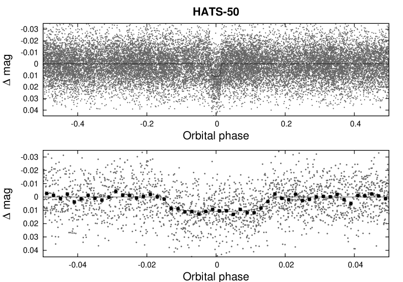
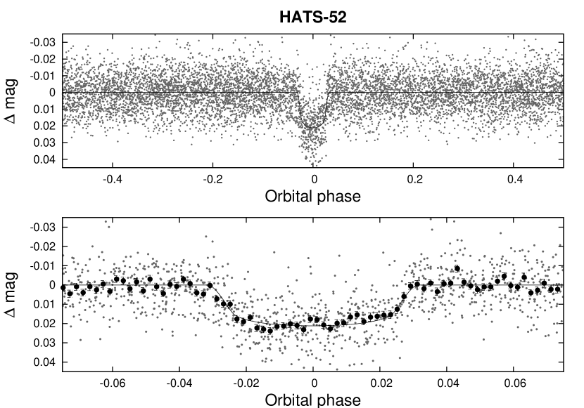
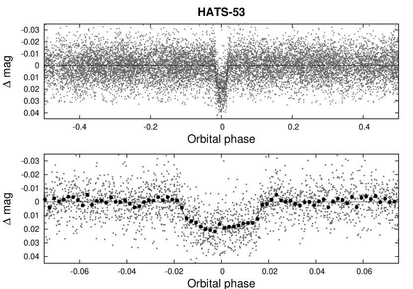
Figure 1: Phase-folded unbinned HATSouth light curves for HATS-50 (upper left), HATS-51 (upper right), HATS-52 (lower left) and HATS-53 (lower right). In each case we show two panels. The top panel shows the full light curve, while the bottom panel shows the light curve zoomed-in on the transit. The solid lines show the model fits to the light curves. The dark filled circles in the bottom panels show the light curves binned in phase with a bin size of 0.002.

Figure 2: Search for additional periodic signals in the light curve of HATS-50 due to other transiting planets. Top panel: BLS spectrum. Bottom panel: Unbinned light curve of HATS-50 (grey points) phase folded with the $0.76624822$ days transit signal. The green points are the phase-binned values (bin size of 0.001). The line is a Mandel & Agol (2002) transit-model fit to the light curve.

After having detected the planetary signals, we further analyze each of the four data sets to search for potential stellar variability/activity and additional periodic signals due to other transiting planets. This analysis was carried out by running BLS on the residuals of each HATSouth light curve, and studying the Generalized Lomb-Scargle periodogram (GLS; Zechmeister & Kürster, 2009). The results of these additional checks are the following.

• By running BLS, we did not detected any significant periodic transit signal in the residuals of the HATS-51, HATS-52 and HATS-53 light curves. For the case of HATS-50, we noticed a marginal transit signal with a period of $0.76624822$ days, $T_{\rm C}=2455274.38586$, depth of $3.2$ mmag, and duration of 46 minutes (bottom panel of Fig. 2). The candidate transit signal has a S/N of 7.5 in the phase-folded light curve and a BLS Signal-Detection-Efficiency (SDE) value of 7.38. Even though this signal is below our threshold for selecting candidates to follow-up (top panel of Fig. 2), it is worth noting it given the presence of the confirmed hot Jupiter and the possibility of close companions to hot-Jupiters (Becker et al., 2015). Therefore, HATS-50 could be an interesting target for a further short-cadence, time-series photometric monitoring with a more precise instrument, like TESS (Ricker et al., 2017). However, given the density of the host star HATS-50, inferred from modelling the transits of HATS-50b (see Table 5), and the duration of the transits for the candidate signal, the candidate planet would have an orbital inclination that differs by more than 10^∘ from that of the hot Jupiter. We finally note that a Mandel & Agol (2002) model fit indicates an implied radius in the super-Neptune regime. So, if this signal was really caused by an additional transiting planet, it would be firmly in the Neptune desert.
  

• By running GLS, we did not detect any significant periodic signal in the GLS spectrum of the light curve obtained for HATS-50, HATS-51 and HATS-53. For these three systems, we placed a $95\%$ confidence upper limit of $0.95$ mmag on the amplitude of any periodic signal between 0.01 days and 100 days. For HATS-52, we detected a sinusoidal signal with a periodicity of $P=15.63703\pm 0.00066$ days and an amplitude of $1.23\pm 0.25$ mmag. The peak has a signal-to-noise ratio of $20.3$ in the spectrum, a periodogram value of $\Delta\chi^{2}/\chi^{2}_{0}=0.0054$, and a false alarm probability (FAP), assuming Gaussian white noise, of $2\times 10^{-5}$. We also assessed the FAP of GLS by performing a bootstrap analysis and obtaining a distribution of peak signals. From this, we estimated a more accurate false alarm probability of $9\times 10^{-5}$.

  This sinusoidal periodic signal can be related to the stellar activity and, therefore, presumably indicates its rotation period. However, considering that HATS-52 has a radius of $R_{\star}=1.046\pm 0.058\,R_{\sun}$ (see Table 5), this value of $P$ implies that $v_{\rm eq}=3.60\pm 0.59$ $\rm km\,s^{-1}$ for HATS-52, which is $1.5\sigma$ below the spectroscopically determined value of $v\sin{i}=4.59\pm 0.64$ $\rm km\,s^{-1}$. So, there is a slight tension between these measurements if we identify the photometric periodicity of $P=15.6$ days with the rotation period of the star.

Table 1: Summary of photometric observations

Instrument/Field	Date(s)	# Images	Cadence	Filter	Precision
			(sec)		(mmag)
HATS-50
HS-2.4/G580	2010 Mar–2011 Aug	6072	294	$r$	12.6
HS-4.4/G580	2010 Mar–2011 Aug	3082	298	$r$	13.2
HS-6.4/G580	2010 Mar–2011 May	742	297	$r$	14.1
HS-1.3/G625	2012 Jun–2012 Oct	4662	291	$r$	13.2
HS-3.3/G625	2012 Jun–2012 Oct	5357	293	$r$	13.0
HS-5.3/G625	2012 Jun–2012 Oct	1724	293	$r$	12.7
PEST 0.3 m	2014 Aug 04	202	133	$R_{c}$	4.8
LCOGT 1 m+CTIO/sinistro	2015 May 11	57	226	$i$	1.3
LCOGT 1 m+SAAO/SBIG	2015 Jun 06	136	150	$i$	4.1
HATS-51
HS-1.2/G601	2011 Aug–2012 Jan	4806	296	$r$	6.2
HS-3.2/G601	2011 Aug–2012 Jan	4062	296	$r$	6.6
HS-5.2/G601	2011 Aug–2012 Jan	3083	290	$r$	6.8
LCOGT 1 m+CTIO/sinistro	2014 Oct 31	36	228	$i$	0.8
LCOGT 1 m+SSO/SBIG	2015 Mar 07	172	76	$i$	2.9
LCOGT 1 m+SAAO/SBIG	2015 Mar 10	92	141	$i$	1.7
LCOGT 1 m+CTIO/sinistro	2015 Oct 03	71	159	$i$	1.8
HATS-52
HS-2.1/G606	2012 Feb–2012 Jun	3753	291	$r$	9.1
HS-4.1/G606	2012 Feb–2012 Jun	2778	300	$r$	11.8
HS-6.1/G606	2012 Feb–2012 Jun	1184	299	$r$	9.8
PEST 0.3 m	2015 Feb 06	193	132	$R_{C}$	12.8
LCOGT 1 m+CTIO/sinistro	2015 May 12	38	226	$i$	4.1
LCOGT 1 m+SSO/SBIG	2015 May 13	53	195	$i$	1.4
LCOGT 1 m+CTIO/sinistro	2015 May 16	42	226	$i$	1.9
LCOGT 1 m+CTIO/sinistro	2015 Oct 23	100	54	$i$	6.4
HATS-53
HS-2.4/G610	2011 Apr–2013 Jul	5496	280	$r$	10.8
HS-4.4/G610	2013 Jan–2013 Jul	3739	323	$r$	10.8
HS-6.4/G610	2011 Apr–2013 Jul	3578	282	$r$	11.8
LCOGT 1 m+CTIO/sinistro	2016 Feb 02	89	219	$i$	1.6
LCOGT 1 m+SAAO/SBIG	2016 Feb 10	48	192	$i$	2.0
PEST 0.3 m	2016 Feb 14	156	132	$R_{C}$	11.9

2.4 Spectroscopic Observations

Table 2: Summary of spectroscopy observations

Instrument	UT Date(s)	# Spec.	Res.	S/N Range	$\gamma_{\rm RV}$	RV Precision
			$\Delta\lambda$/$\lambda$/1000		($\rm km\,s^{-1}$)	($\rm m\,s^{-1}$)
HATS-50
ANU 2.3 m/WiFeS	2014 Jun 3–5	3	7	21–90	-23.4	4000
ANU 2.3 m/WiFeS	2014 Jun 4	1	3	76	$\cdots$	$\cdots$
Euler 1.2 m/CORALIE	2014 Jun–Sep	4	60	7–13	-20.176	73
MPG 2.2 m/FEROS	2014 Jul–2016 Sep	32	48	14–55	-20.250	72
Keck-I 10 m/HIRES+I2	2014 Sep–2015 Jul	7	48	110–155	$\cdots$	29
Keck-I 10 m/HIRES	2015 Jul 5	1	48	70	$\cdots$	$\cdots$
HATS-51
ANU 2.3 m/WiFeS	2014 Oct 7	1	3	46	$\cdots$	$\cdots$
ANU 2.3 m/WiFeS	2014 Oct 8–12	4	7	33–67	2.0	4000
Euler 1.2 m/CORALIE	2014 Oct–2016 Nov	24	60	8–30	3.086	55
MPG 2.2 m/FEROS	2014 Dec–2015 Feb	14	48	60–97	3.087	55
AAT 3.9 m/CYCLOPS	2015 Feb–May	13	70	$\cdots$	3.087	30
HATS-52
ANU 2.3 m/WiFeS	2014 Jul 3	1	3	58	$\cdots$	$\cdots$
ANU 2.3 m/WiFeS	2014 Jul–2015 Jan	4	7	14–50	13.8	4000
Euler 1.2 m/CORALIE	2015 Mar 28	1	60	11	13.30	$\cdots$
ESO 3.6 m/HARPS	2015 Apr 6–8	3	115	10–13	13.384	15
MPG 2.2 m/FEROS	2015 Jun–2016 Feb	11	48	25–48	13.456	127
HATS-53
ANU 2.3 m/WiFeS	2015 Mar 30	1	3	30	$\cdots$	$\cdots$
ANU 2.3 m/WiFeS	2015 Mar–Apr	2	7	6–33	68.5	4000
ESO 3.6 m/HARPS	2015 Apr 7–8	2	115	7–12	71.945	23
MPG 2.2 m/FEROS	2015 Jun 6–20	11	48	21–40	71.950	28

Table 3: Relative radial velocities and bisector spans for HATS-50–HATS-53.

BJD	RV	$\sigma_{\rm RV}$	BS	$\sigma_{\rm BS}$	Phase	Instrument
(2,450,000$+$)	($\rm m\,s^{-1}$)	($\rm m\,s^{-1}$)	($\rm m\,s^{-1}$)	($\rm m\,s^{-1}$)
HATS-50
$6828.86592$	$-17.38$	$24.00$	$75.0$	$37.0$	$0.168$	Coralie
$6829.74512$	$24.62$	$26.00$	$118.0$	$43.0$	$0.398$	Coralie
$6857.78434$	$68.26$	$12.00$	$9.0$	$15.0$	$0.719$	FEROS
$6858.73766$	$14.26$	$11.00$	$11.0$	$14.0$	$0.968$	FEROS
$6859.76731$	$-56.74$	$12.00$	$4.0$	$16.0$	$0.237$	FEROS
$6862.68928$	$144.26$	$33.00$	$50.0$	$41.0$	$0.000$	FEROS
$6907.82693$	$58.01$	$4.95$	$\cdots$	$\cdots$	$0.786$	HIRES
$6908.75386$	$31.96$	$5.67$	$\cdots$	$\cdots$	$0.028$	HIRES
$6909.74379$	$-4.97$	$11.27$	$\cdots$	$\cdots$	$0.287$	HIRES
$6911.50060$	$-62.38$	$41.00$	$-301.0$	$63.0$	$0.746$	Coralie
$6911.76564$	$49.40$	$4.49$	$\cdots$	$\cdots$	$0.815$	HIRES
$6912.49456$	$-62.38$	$30.00$	$-178.0$	$51.0$	$0.005$	Coralie
$6912.79856$	$-36.69$	$4.79$	$\cdots$	$\cdots$	$0.084$	HIRES
$6913.78648$	$-68.78$	$5.12$	$\cdots$	$\cdots$	$0.342$	HIRES
$6932.53890$	$-176.74$	$13.00$	$-75.0$	$17.0$	$0.239$	FEROS
$6942.60598$	$0.26$	$13.00$	$-29.0$	$16.0$	$0.868$	FEROS
$6983.54362$	$67.26$	$11.00$	$23.0$	$15.0$	$0.557$	FEROS
$7166.81632$	$-64.74$	$15.00$	$-30.0$	$19.0$	$0.413$	FEROS
$7181.70212$	$-3.74$	$14.00$	$8.0$	$18.0$	$0.300$	FEROS
$7186.89313$	$112.26$	$18.00$	$75.0$	$24.0$	$0.655$	FEROS
$7188.70636$	$-22.74$	$13.00$	$15.0$	$18.0$	$0.129$	FEROS
$7209.04868$	$1.46$	$6.60$	$\cdots$	$\cdots$	$0.440$	HIRES
$7211.80755$	$-45.74$	$12.00$	$21.0$	$16.0$	$0.161$	FEROS
$7219.64476$	$-47.74$	$12.00$	$-19.0$	$17.0$	$0.207$	FEROS
$7223.64984$	$6.26$	$15.00$	$36.0$	$20.0$	$0.253$	FEROS
$7225.55693$	$62.26$	$11.00$	$-11.0$	$15.0$	$0.751$	FEROS
$7227.54760$	$-73.74$	$13.00$	$-41.0$	$17.0$	$0.271$	FEROS
$7235.52005$	$-191.74$	$34.00$	$99.0$	$20.0$	$0.352$	FEROS
$7236.84001$	$-114.74$	$17.00$	$129.0$	$19.0$	$0.697$	FEROS
$7297.66592$	$-52.74$	$18.00$	$-177.0$	$24.0$	$0.580$	FEROS
$7299.64213$	$-83.74$	$16.00$	$-16.0$	$22.0$	$0.096$	FEROS
$7557.80118$	$62.26$	$12.00$	$-28.0$	$17.0$	$0.505$	FEROS
$7558.81095$	$80.26$	$12.00$	$33.0$	$17.0$	$0.769$	FEROS
$7569.65730$	$106.26$	$15.00$	$93.0$	$22.0$	$0.601$	FEROS
$7576.64710$	$41.26$	$16.00$	$39.0$	$21.0$	$0.426$	FEROS
$7590.72922$	$-25.94$	$10.50$	$22.0$	$14.0$	$0.103$	FEROS
$7593.67838$	$4.86$	$12.90$	$54.0$	$17.0$	$0.874$	FEROS
$7612.71943$	$113.86$	$12.30$	$6.0$	$17.0$	$0.845$	FEROS
$7614.57198$	$79.66$	$12.60$	$127.0$	$16.0$	$0.329$	FEROS

HATS-51    $6939.83172$ $-15.58$ $17.00$ $-11.0$ $27.0$ $0.491$ Coralie $6940.81069$ $104.42$ $63.00$ $5.0$ $68.0$ $0.783$ Coralie $6941.86563$ $-73.58$ $19.00$ $-60.0$ $29.0$ $0.098$ Coralie $6967.78670$ $132.42$ $19.00$ $116.0$ $29.0$ $0.838$ Coralie $6969.79828$ $30.42$ $18.00$ $23.0$ $27.0$ $0.439$ Coralie $6972.69347$ $-50.58$ $16.00$ $65.0$ $25.0$ $0.303$ Coralie $6997.69160$ $178.26$ $10.00$ $87.0$ $12.0$ $0.768$ FEROS $6997.73191$ $201.26$ $10.00$ $74.0$ $13.0$ $0.780$ FEROS $6999.63851$ $-9.74$ $10.00$ $38.0$ $11.0$ $0.349$ FEROS $7030.81040$ $36.26$ $10.00$ $2.0$ $10.0$ $0.657$ FEROS $7033.73624$ $3.26$ $10.00$ $9.0$ $10.0$ $0.531$ FEROS $7035.75138$ $-68.74$ $10.00$ $-4.0$ $11.0$ $0.133$ FEROS $7036.67747$ $-49.74$ $10.00$ $6.0$ $10.0$ $0.409$ FEROS $7037.79634$ $59.26$ $10.00$ $12.0$ $10.0$ $0.744$ FEROS $7049.60146$ $-96.74$ $10.00$ $-22.0$ $10.0$ $0.269$ FEROS $7050.67770$ $34.26$ $10.00$ $12.0$ $10.0$ $0.590$ FEROS $7053.74327$ $-17.74$ $10.00$ $-18.0$ $10.0$ $0.505$ FEROS $7054.60465$ $61.26$ $10.00$ $-5.0$ $10.0$ $0.763$ FEROS $7055.64520$ $-94.74$ $10.00$ $-65.0$ $10.0$ $0.073$ FEROS $7057.74745$ $8.26$ $10.00$ $-85.0$ $11.0$ $0.701$ FEROS $7075.63657$ $-61.58$ $18.00$ $6.0$ $29.0$ $0.043$ Coralie $7076.65198$ $-86.58$ $18.00$ $-2.0$ $29.0$ $0.346$ Coralie $7078.63334$ $-0.58$ $18.00$ $-46.0$ $29.0$ $0.938$ Coralie $7080.99763$ $18.92$ $9.40$  $\cdots$   $\cdots$  $0.644$ CYCLOPS $7081.01370$ $42.82$ $6.40$  $\cdots$   $\cdots$  $0.649$ CYCLOPS $7081.07820$ $59.12$ $8.60$  $\cdots$   $\cdots$  $0.668$ CYCLOPS $7082.97896$ $-58.38$ $9.00$  $\cdots$   $\cdots$  $0.235$ CYCLOPS $7082.99492$ $-49.68$ $7.60$  $\cdots$   $\cdots$  $0.240$ CYCLOPS $7083.01087$ $-34.78$ $11.70$  $\cdots$   $\cdots$  $0.245$ CYCLOPS $7149.86599$ $-104.58$ $13.50$  $\cdots$   $\cdots$  $0.208$ CYCLOPS $7149.89323$ $-100.98$ $13.00$  $\cdots$   $\cdots$  $0.217$ CYCLOPS $7149.90918$ $-123.48$ $20.90$  $\cdots$   $\cdots$  $0.221$ CYCLOPS $7152.85935$ $-57.48$ $12.10$  $\cdots$   $\cdots$  $0.102$ CYCLOPS $7152.86772$ $-72.48$ $20.40$  $\cdots$   $\cdots$  $0.105$ CYCLOPS $7154.86321$ $77.12$ $5.30$  $\cdots$   $\cdots$  $0.701$ CYCLOPS $7154.87917$ $113.72$ $6.70$  $\cdots$   $\cdots$  $0.705$ CYCLOPS $7313.71457$ $-4.58$ $18.00$ $147.0$ $49.0$ $0.135$ Coralie $7317.75708$ $-228.58$ $19.00$ $-74.0$ $38.0$ $0.342$ Coralie $7318.73072$ $53.42$ $18.00$ $-27.0$ $38.0$ $0.633$ Coralie $7408.69120$ $-28.58$ $12.00$ $16.0$ $20.0$ $0.496$ Coralie $7409.69015$ $14.42$ $12.00$ $10.0$ $20.0$ $0.794$ Coralie $7410.58904$ $82.42$ $14.00$ $-92.0$ $23.0$ $0.063$ Coralie $7411.54533$ $-88.58$ $19.00$ $-141.0$ $32.0$ $0.348$ Coralie $7464.64412$ $-70.58$ $17.00$ $-54.0$ $32.0$ $0.204$ Coralie $7466.52399$ $82.42$ $17.00$ $25.0$ $29.0$ $0.765$ Coralie $7640.86434$ $63.42$ $16.00$ $23.0$ $29.0$ $0.825$ Coralie $7643.82622$ $61.42$ $13.00$ $-23.0$ $26.0$ $0.709$ Coralie $7645.89470$ $-50.58$ $12.00$ $4.0$ $22.0$ $0.327$ Coralie    HATS-52    $7109.65449$ $-323.80$ $34.00$ $\cdots$ $\cdots$ $0.165$ Coralie $7118.61984$ $378.20$ $24.00$ $-15.0$ $31.0$ $0.725$ HARPS $7119.61676$ $-82.80$ $31.00$ $95.0$ $37.0$ $0.455$ HARPS $7120.59836$ $-341.80$ $28.00$ $-8.0$ $37.0$ $0.173$ HARPS $7181.53193$ $324.38$ $24.00$ $-136.0$ $24.0$ $0.759$ FEROS $7185.51437$ $228.38$ $25.00$ $-24.0$ $24.0$ $0.673$ FEROS $7186.48111$ $-235.62$ $22.00$ $125.0$ $21.0$ $0.380$ FEROS $7187.48351$ $-333.62$ $25.00$ $-36.0$ $24.0$ $0.114$ FEROS $7190.47681$ $-355.62$ $24.00$ $53.0$ $24.0$ $0.304$ FEROS $7324.83438$ $566.38$ $19.00$ $146.0$ $18.0$ $0.615$ FEROS $7325.84444$ $-219.62$ $15.00$ $86.0$ $15.0$ $0.354$ FEROS $7327.85022$ $386.38$ $18.00$ $137.0$ $18.0$ $0.822$ FEROS $7403.83591$ $-196.62$ $15.00$ $16.0$ $15.0$ $0.422$ FEROS $7405.78818$ $330.38$ $17.00$ $33.0$ $17.0$ $0.850$ FEROS $7447.77082$ $-15.62$ $18.00$ $-107.0$ $18.0$ $0.570$ FEROS    HATS-53    $7119.69799$ $57.38$ $45.00$ $-77.0$ $53.0$ $0.625$ HARPS $7120.69688$ $86.38$ $19.00$ $-83.0$ $29.0$ $0.884$ HARPS $7181.59141$ $72.23$ $16.00$ $54.0$ $21.0$ $0.686$ FEROS $7182.52590$ $28.23$ $14.00$ $-17.0$ $18.0$ $0.928$ FEROS $7183.59764$ $-86.77$ $14.00$ $13.0$ $18.0$ $0.206$ FEROS $7184.48225$ $-9.77$ $15.00$ $15.0$ $19.0$ $0.436$ FEROS $7185.62553$ $103.23$ $21.00$ $-43.0$ $28.0$ $0.732$ FEROS $7186.57088$ $62.23$ $18.00$ $-63.0$ $24.0$ $0.978$ FEROS $7187.63960$ $-48.77$ $18.00$ $-63.0$ $24.0$ $0.255$ FEROS $7190.53242$ $-32.77$ $15.00$ $-65.0$ $19.0$ $0.006$ FEROS $7192.50171$ $-36.77$ $21.00$ $-98.0$ $28.0$ $0.517$ FEROS $7193.61040$ $82.23$ $15.00$ $6.0$ $19.0$ $0.804$ FEROS $7194.49223$ $-27.77$ $14.00$ $16.0$ $17.0$ $0.033$ FEROS

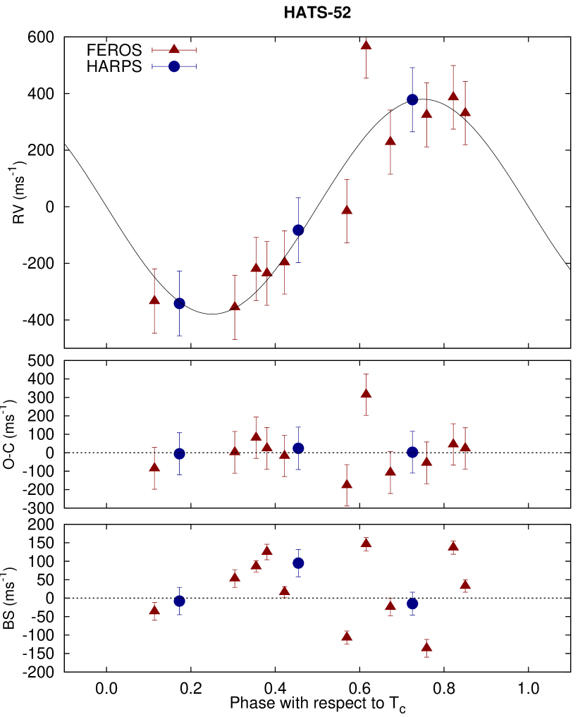
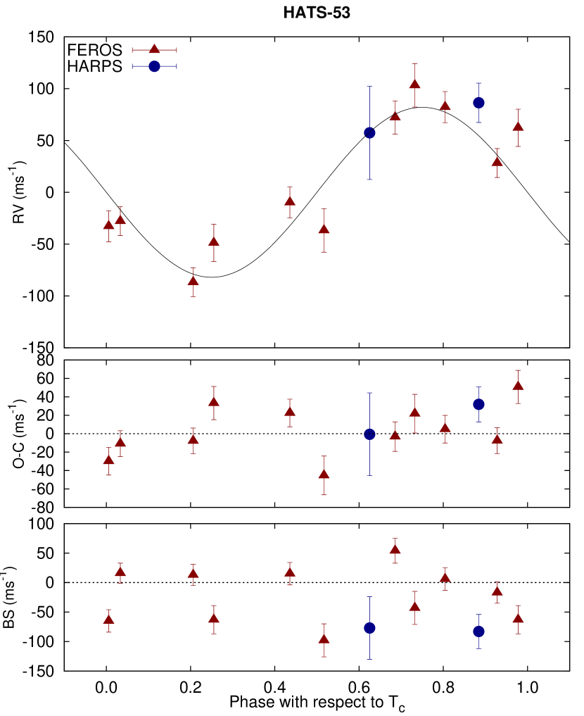
Figure 3: Phased high-precision RV measurements for HATS-50 (upper left), HATS-51 (upper right), HATS-52 (lower left) and HATS-53 (lower right). The instruments used are labelled in the plots. In each case we show three panels. The top panel shows the phased measurements together with our best-fit model (see Table 6) for each system. Zero-phase corresponds to the time of mid-transit. The center-of-mass velocity has been subtracted. The second panel shows the velocity $O\!-\!C$ residuals from the best fit. The error bars include the jitter terms listed in Table 6 added in quadrature to the formal errors for each instrument. The third panel shows the bisector spans (BS). Note the different vertical scales of the panels.

The first step that was undertaken in confirming the planetary nature of the four planetary candidates was to obtain a spectral reconnaissance of their host stars. This allows us to rule out the usual false positive cases (giant stars, binary systems, and blending with faint eclipsing-binary systems). For this purpose, we used the Wide Field Spectrograph (WiFeS; Dopita et al., 2007), mounted on the ANU 2.3 m telescope at SSO. The spectroscopic parameters were estimated by taking low-resolution spectra ($R=3000$). All the four targets were identified as dwarf stars. We also took medium-resolution spectra ($R=7000$), with the aim to search for possible RV variations at the $\sim 2$ km s^-1 level, which are useful to rule out possible stellar companions. Details about the data reduction and the processing of the WiFeS spectra are summarized in Bayliss et al. (2013).

Precise RV measurements of the targets were then acquired by using several medium- and large-class telescopes, equipped with high-resolution spectrographs and working on wide ranges of optical wavelengths. They are summarized in Table 2, together with their main characteristics. With these instruments, it was possible to measure periodic RV variation of the stars, which is compatible with the presence of planet-type objects orbiting around them. In particular, we mainly used the FEROS spectrograph (Kaufer & Pasquini, 1998), which is mounted on the MPG 2.2 m telescope at the ESO Observatory in La Silla, for monitoring the four targets. Other spectra were collected thanks to CORALIE (Queloz et al., 2001) on the Euler 1.2 m telescope, HARPS (Mayor et al., 2003) on the ESO 3.6 m telescope, which are also located at the La Silla observatory, and CYCLOPS mounted on the 3.9 m Anglo-Australian Telescope at SSO. For the case of HATS-50, which is the faintest star of the four ($V=14.0$ mag), we needed higher signal-to-noise (S/N) measurements. These were obtained by taking seven spectra with the HIRES spectrograph (Vogt et al., 1994) on the Keck-I 10 m telescope at Mauna Kea Observatory in Hawaii.

More details about the instruments, the data reduction and the computation of the corresponding RVs can be found in the previous works of the HATSouth team, e.g. Penev et al. (2013); Mohler-Fischer et al. (2013); Bayliss et al. (2013). In particular, HARPS, FEROS and CORALIE spectra were analysed with the method described in Jordán et al. (2014) and Brahm et al. (2017b), while those coming from CYCLOPS in Addison et al. (2013). Finally, we refer the reader to Bakos et al. (2015) and Howard et al. (2010) for the analysis of the Keck/HIRES spectra.

The values of the RV measurements are reported in Table 2.4, while the phased RVs and bisector spans (BS) are plotted for each system in Figure 3. We also used the FEROS high-resolution spectra for an accurate determination of the stellar spectroscopic parameters (effective temperature, metal abundance and projected rotational velocity) by applying the ZASPE (Zonal Atmospherical Stellar Parameter Estimator) routine (Brahm et al., 2017a). This analysis is discussed in Sect. 3.1.

2.5 Photometric follow-up observations

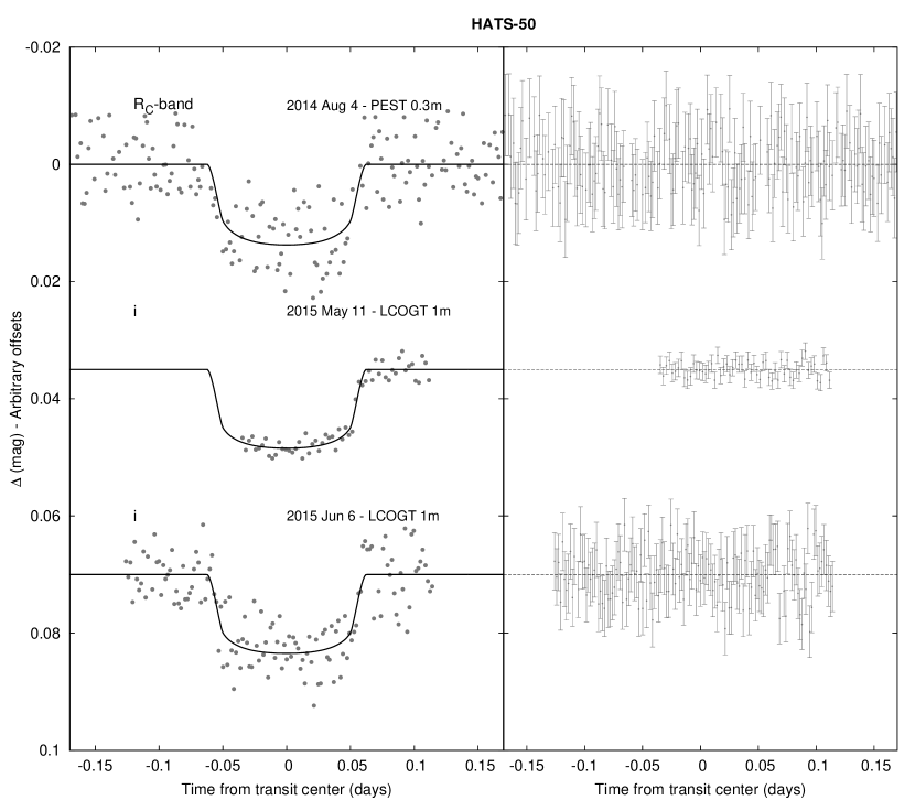
Figure 4: Unbinned transit light curves for HATS-50. The light curves have been corrected for quadratic trends in time, and linear trends with up to three parameters characterizing the shape of the PSF, fitted simultaneously with the transit model. The dates of the events, filters and instruments used are indicated. Light curves following the first are displaced vertically for clarity. Our best fit from the global modeling described in Section 3.3 is shown by the solid lines. The residuals from the best-fit model are shown on the right-hand-side in the same order as the original light curves. The error bars represent the photon and background shot noise, plus the readout noise.

Figure 5: Same as Fig. 4, here we show light curves for HATS-51.

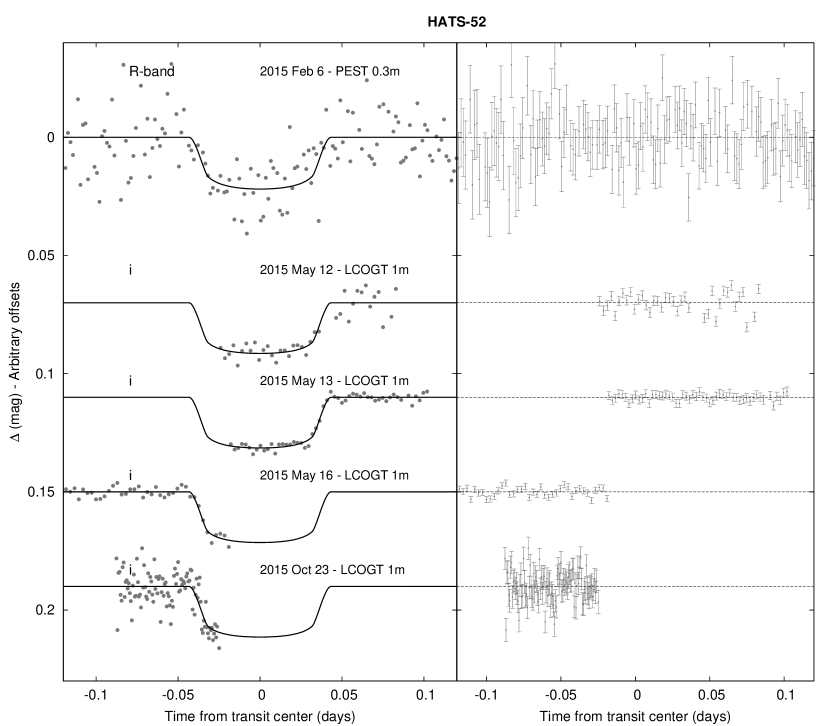
Figure 6: Same as Fig. 4, here we show light curves for HATS-52.

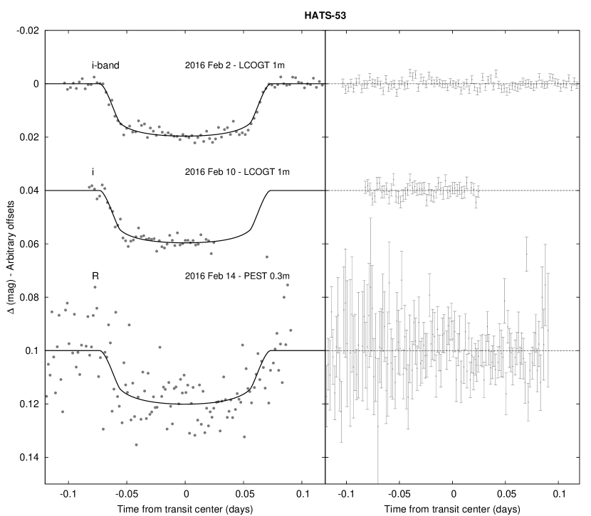
Figure 7: Same as Fig. 4, here we show light curves for HATS-53.

Another important step for confirming and characterizing a transiting exoplanetary system consists of performing photometric follow-up observations of transit events. We can thus derive more precise measurements, with respect to the survey data, of the transit depth, duration, mid-transit time and contact points of the corresponding light curves. An accurate knowledge of these photometric parameters are vital for robustly constraining the orbital parameters of the system and the physical parameters of both the star and the planet.

One complete transit event was observed with the PEST 0.3 m telescope for HATS-50b, HATS-52b, and HATS-53b through a $R$-band filter. Details of this telescope and the method used for reducing the data are described in Zhou et al. (2014). Other eleven transit light curves of the four targets were recorded using the 1-m telescopes (CTIO, SAAO, SSO) in the Las Cumbres Observatory Global Telescope network (LCOGT: Brown et al., 2013) and Sloan-$i^{\prime}$ filters. The LCOGT telescopes and the corresponding data reduction are described in Hartman et al. (2015). An excerpt of these observations is reported in Table 1. The light curves are plotted in Figures 4, 5, 6, and 7, for HATS-50, HATS-51, HATS-52, and HATS-53, respectively, and are compared to our best-fit models.

Table 4: Light curve data for HATS-50, HATS-51, HATS-52 and HATS-53.

Note. — This table is available in a machine-readable form in the online journal. A portion is shown here for guidance regarding its form and content.

2.6 Lucky Imaging

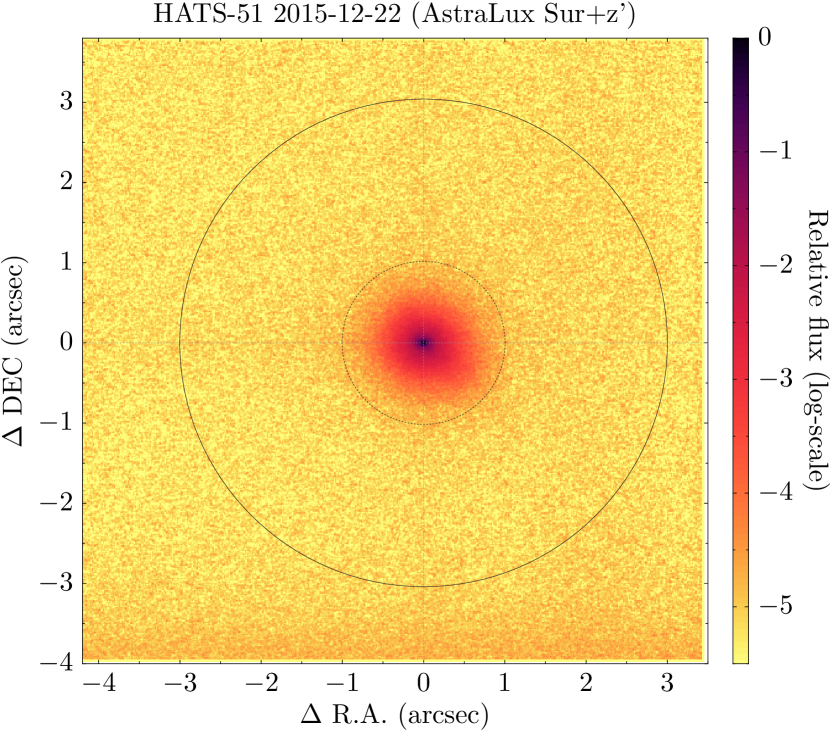
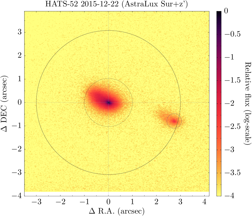
Figure 8: Astralux lucky images of HATS-51 (left) and HATS-52 (right). No neighboring source is detected for HATS-51. For HATS-52 a neighbor is clearly detected at $\Delta{\rm R.A.}\approx 3^{\arcsec}$, $\Delta{\rm Dec.}\approx-1^{\arcsec}$ and with $\Delta z^{\prime}=2.457\pm 0.013$ mag.

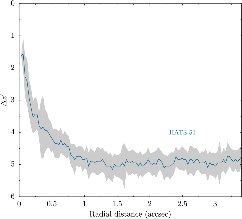
Figure 9: Contrast curves for HATS-51 (left), and HATS-52 (right) based on our AstraLux Sur $z^{\prime}-band$ observations. Gray bands show the uncertainty given by the scatter in the contrast in the azimuthal direction at a given radius. The neighbor to HATS-52 is marked with the red filled circle.

Lucky imaging observations were obtained through a $z^{\prime}$ filter for the HATS-51 and HATS-52 systems using the Astralux Sur camera (Hippler et al., 2009) on the New Technology Telescope (NTT), at La Silla Observatory in Chile, on the nights of 2015 December 22 and 23. Observations with this facility were carried out and reduced following Espinoza et al. (2016), but a plate scale of 15.20 mas pixel^-1 (derived in the work of Janson et al., 2017) was used. Figure 8 shows the reduced final images for each system, while Figure 9 shows the contrast curves based on these images produced using the technique and software described in Espinoza et al. (2016).

For HATS-52 a neighboring source is clearly detected at a distance of $2.74\pm 0.03$ arcsec to the east and $0.79\pm 0.03$ arcsec to the south from the target (i.e., at a distance of $2.85\pm 0.03$ arcsec from the target), with $\Delta z^{\prime}=2.457\pm 0.013$ mag, relative to the target. Based on the photometric follow-up observations of this system that were carried out with the LCOGT 1 m telescope network (Section 2.5), we were able to determine that the transits occur around the star HATS-52, and not the neighbor. The final combined image has an effective FWHM of $0\farcs 0722\pm 0\farcs 0050$. The same source was detected by the GAIA space observatory (GAIA Data Release 1; Linegren et al., 2016) at $\approx 2\farcs 8$ separation to the East from HATS-52, with $\Delta G_{\rm GAIA}=2.26$. Closer sources were not detected.

For HATS-51 no neighbors were detected with the Astralux Sur camera (effective FWHM of $0\farcs 0431\pm 0\farcs 0053$), neither with GAIA within $10^{\prime\prime}$. Instead, based on GAIA data, we report that HATS-50 has a neighbor at $2\farcs 1$ to the east ($\Delta\,G=2.97$), while HATS-53 has no neighbors within $8\farcs$.

3 Analysis

Here we describe the analysis of the observational data, which were presented in the previous section, with the aim to get complete physical characterizations of the HATS-50, HATS-51, HATS-52 and HATS-53 planetary systems.

3.1 Properties of the parent star

As anticipated before, we used high-resolution FEROS spectra for determining the atmospheric properties (metallicity, effective temperature and surface gravity) of the four stars. The spectra were analysed with the ZASPE routine, which is comprehensively described in Brahm et al. (2017a).

Then, we followed the methodology of Sozzetti et al. (2007) for determining other stellar parameters (mass, radius, luminosity, age, etc.) together with their uncertainties. In brief, we performed a Markov chain Monte Carlo (MCMC) global analysis of our photometric and spectroscopic data, based on ($i$) the stellar effective temperature, $T_{\rm eff\star}$, and stellar metal abundance, [Fe/H], which were both determined with ZASPE, ($ii$) the stellar mean density, $\rho_{\star}$, estimated by modelling the photometric transit light curves, and ($iii$) using the Yonsei-Yale (YY; Yi et al., 2001) evolutionary tracks.

We determined the YY isochrones for each of the four systems over a wide range of ages. The values of the stellar parameters were obtained from the best agreement between the resulting values of $\rho_{\star}$ and $T_{\rm eff\star}$ and those estimated from the data. Figure 10 shows the locations of each star on an $T_{\rm eff\star}$–$\rho_{\star}$ diagram. From this analysis, we kept the values of the stellar logarithmic surface gravities, $\log{g_{\star}}$, and used them as fixed parameters for a second iteration with ZASPE, which returned the final values of the parameters of the four stars. They are reported in Table 5 and all our objects are G-type stars.

The most likely values for $T_{\rm eff\star}$ and $\rho_{\star}$ for HATS-52 fall at a higher density than the lowest age isochrone tabulated in the models (see bottom-left panel in Figure 10). The models and observations are consistent within $2\sigma$. For determining the physical parameters of this star we exclude any $T_{\rm eff\star}$-$\rho_{\star}$-$\rm[Fe/H]$ point in the Markov chain which does not match to a stellar model. In Table 5 we list for each star the median stellar density based both on the full Mark chain (i.e., without enforcing a match to the stellar models) and on the chain after excluding points that do not match to a model.

We note that, while HATS-53 has physical characteristics similar to the Sun ($T_{\rm eff\star}=5644\pm 94$, $\rm[Fe/H]=0.010\pm 0.066$, $M_{\star}=0.964\pm 0.040\,M_{\sun}$, $R_{\star}=1.101_{-0.024}^{+0.031}\,R_{\sun}$), HATS-50, HATS-51 and HATS-52 are more massive, larger, and metal richer ($\rm[Fe/H]=0.300\pm 0.056$, $\rm[Fe/H]=0.300\pm 0.030$ and $\rm[Fe/H]=0.22\pm 0.10$ for HATS-50, HATS-51 and HATS-52, respectively). We note that HATS-51 is much less dense ($\rho_{\star}=0.56_{-0.16}^{+0.22}\,$g cm^-3) than the other three stars due to its large radius ($R_{\star}=1.44\pm 0.18\,R_{\sun}$). Moreover, our analysis indicates that HATS-50 and HATS-52 are quite young, i.e. $1.2\pm 1.1$ Gyr and $1.2_{-1.1}^{+1.5}$ Gyr, respectively; these estimates are both consistent with their Zero Age Main Sequence implying a $95\%$ confidence upper limit on the age of $t<3.9$ Gyr and $t<3.8$ Gyr, for HATS-50 and HATS-52 respectively. HATS-51 has an intermediate age ($4.74_{-0.51}^{+0.70}$ Gyr), whereas HATS-53 is quite old ($9.0\pm 1.9$ Gyr).

We also estimated the distance of the four stars by comparing their broad-multi-band photometry taken from public astronomical archives (see Table 5) with the predicted magnitudes in each filter from the isochrones. The extinction was determined assuming a $R_{V}=3.1$ law from Cardelli et al. (1989). For a consistency check, we used the NED online extinction calculator, based on Galactic extinction maps, for estimating the expected total line of site extinction for each source. Three of them (HATS-51, HATS-52 and HATS-53) passed this check, as we found values greater than the inferred $A_{V}$. In the case of HATS-50, our estimated $A_{V}$ is very close to the value determined from the dust maps.

Figure 10: Model isochrones from Yi et al. (2001) for the measured metallicities of HATS-50 (upper left), HATS-51 (upper right), HATS-52 (lower left) and HATS-53 (lower right). We show models for ages of 0.2 Gyr and 1.0 to 14.0 Gyr in 1.0 Gyr increments (ages increasing from left to right). The adopted values of $T_{\rm eff\star}$ and $\rho_{\star}$ are shown together with their 1$\sigma$ and 2$\sigma$ confidence ellipsoids. The initial values of $T_{\rm eff\star}$ and $\rho_{\star}$ from the first ZASPE and light curve analyses of HATS-50 and HATS-53 are represented with open triangles.

Table 5: Stellar parameters for HATS-50–HATS-53

	HATS-50	HATS-51	HATS-52	HATS-53
Parameter	Value	Value	Value	Value	Source
Astrometric properties and cross-identifications
2MASS-ID	20014273-2604392	06512340-2903309	09202105-3116095	11463084-3351361
GSC-ID	GSC 6896-01012	GSC 6534-00607	GSC 7153-01785	GSC 7225-00413
R.A. (J2000)	$20^{\mathrm{h}}01^{\mathrm{m}}42.60{\mathrm{s}}$	$06^{\mathrm{h}}51^{\mathrm{m}}23.40{\mathrm{s}}$	$09^{\mathrm{h}}20^{\mathrm{m}}21.05{\mathrm{s}}$	$11^{\mathrm{h}}46^{\mathrm{m}}30.72{\mathrm{s}}$	2MASS
Dec. (J2000)	$-26{\arcdeg}04{\arcmin}39.3{\arcsec}$	$-29{\arcdeg}03{\arcmin}31.0{\arcsec}$	$-31{\arcdeg}16{\arcmin}09.6{\arcsec}$	$-33{\arcdeg}51{\arcmin}36.2{\arcsec}$	2MASS
$\mu_{\rm R.A.}$ ($\rm mas\,yr^{-1}$)	$3.2\pm 1.6$	$-15.5\pm 1.2$	$-27.7\pm 3.7$	$-35.0\pm 2.0$	UCAC4
$\mu_{\rm Dec.}$ ($\rm mas\,yr^{-1}$)	$1.6\pm 1.6$	$-6.9\pm 1.1$	$16.0\pm 3.7$	$-5.0\pm 2.1$	UCAC4
Spectroscopic properties
$T_{\rm eff\star}$ (K)	$5990\pm 110$	$5758\pm 58$	$6010\pm 150$	$5644\pm 94$	ZASPE
$\rm[Fe/H]$	$0.300\pm 0.056$	$0.300\pm 0.030$	$0.22\pm 0.10$	$0.010\pm 0.066$	ZASPE
$v\sin{i}$ ($\rm km\,s^{-1}$)	$3.76\pm 0.54$	$3.98\pm 0.26$	$4.59\pm 0.64$	$2.50\pm 0.76$	ZASPE
$v_{\rm mac}$ ($\rm km\,s^{-1}$)	$4.32\pm 0.17$	$3.962\pm 0.088$	$4.35\pm 0.23$	$3.79\pm 0.14$	Assumed
$v_{\rm mic}$ ($\rm km\,s^{-1}$)	$1.225\pm 0.085$	$1.070\pm 0.034$	$1.24\pm 0.12$	$1.006\pm 0.049$	Assumed
$\gamma_{\rm RV}$ ($\rm m\,s^{-1}$)	$-20250\pm 13$	$3093\pm 15$	$13456\pm 43$	$71949.5\pm 7.1$	FEROS
Photometric properties
$G$ (mag)	13.8	12.24	13.54	13.57	GAIA DR1
$B$ (mag)	$14.718\pm 0.010$	$13.190\pm 0.030$	$14.316\pm 0.030$	$14.548\pm 0.040$	APASS
$V$ (mag)	$14.033\pm 0.050$	$12.471\pm 0.030$	$13.669\pm 0.040$	$13.790\pm 0.030$	APASS
$g$ (mag)	$\cdots$	$12.766\pm 0.030$	$13.962\pm 0.020$	$14.137\pm 0.020$	APASS
$r$ (mag)	$\cdots$	$12.269\pm 0.040$	$13.490\pm 0.060$	$13.579\pm 0.030$	APASS
$i$ (mag)	$13.535\pm 0.010$	$12.115\pm 0.040$	$13.409\pm 0.070$	$13.30\pm 0.28$	APASS
$J$ (mag)	$12.643\pm 0.025$	$11.241\pm 0.023$	$12.523\pm 0.034$	$12.458\pm 0.025$	2MASS
$H$ (mag)	$12.373\pm 0.034$	$10.955\pm 0.024$	$12.218\pm 0.035$	$12.088\pm 0.027$	2MASS
$K_{s}$ (mag)	$12.289\pm 0.027$	$10.867\pm 0.021$	$12.114\pm 0.030$	$12.046\pm 0.027$	2MASS
Derived properties
$M_{\star}$ ($M_{\sun}$)	$1.168\pm 0.042$	$1.187\pm 0.060$	$1.111\pm 0.054$	$0.964\pm 0.040$	YY+$\rho_{\star}$+ZASPE
$R_{\star}$ ($R_{\sun}$)	$1.117\pm 0.060$	$1.44\pm 0.18$	$1.046\pm 0.058$	$1.101_{-0.024}^{+0.031}$	YY+$\rho_{\star}$+ZASPE
$\log{g_{\star}}$ (cgs)	$4.411\pm 0.038$	$4.198\pm 0.088$	$4.445\pm 0.034$	$4.340\pm 0.019$	YY+$\rho_{\star}$+ZASPE
$\rho_{\star}$ ($\rm g\,cm^{-3}$)	$1.38_{-0.23}^{+0.16}$	$0.56_{-0.16}^{+0.21}$	$1.70_{-0.24}^{+0.17}$	$1.026_{-0.071}^{+0.048}$	Light curves
$\rho_{\star}$ ($\rm g\,cm^{-3}$)	$1.19\pm 0.16$	$0.56_{-0.16}^{+0.22}$	$1.37\pm 0.18$	$1.027_{-0.071}^{+0.050}$	YY+Light curves+ZASPE
$L_{\star}$ ($L_{\sun}$)	$1.39\pm 0.23$	$2.04\pm 0.54$	$1.17\pm 0.22$	$1.11\pm 0.11$	YY+$\rho_{\star}$+ZASPE
$M_{V}$ (mag)	$4.44\pm 0.19$	$4.05\pm 0.27$	$4.64\pm 0.22$	$4.74\pm 0.12$	YY+$\rho_{\star}$+ZASPE
$M_{K}$ (mag,ESO)	$3.01\pm 0.13$	$2.51\pm 0.26$	$3.17\pm 0.15$	$3.121\pm 0.066$	YY+$\rho_{\star}$+ZASPE
Age (Gyr)	$1.2\pm 1.1$	$4.74_{-0.51}^{+0.70}$	$1.2_{-1.1}^{+1.5}$	$9.0\pm 1.9$	YY+$\rho_{\star}$+ZASPE
$A_{V}$ (mag)	$0.305\pm 0.098$	$0.024_{-0.024}^{+0.059}$	$0.025_{-0.025}^{+0.108}$	$0.112\pm 0.078$	YY+$\rho_{\star}$+ZASPE
Distance (pc)	$717\pm 43$0	$478\pm 59$	$631\pm 44$	$613\pm 19$	YY+$\rho_{\star}$+ZASPE

Note. — For all four systems we adopt a model in which the orbit is assumed to be circular. See the discussion in Section 3.3.

3.2 Excluding blend scenarios

In order to exclude blend scenarios we carried out an analysis following Hartman et al. (2012). We attempt to model the available photometric data (including light curves and catalog broad-band photometric measurements) for each object as a blend between an eclipsing binary star system and a third star along the line of sight. The physical properties of the stars are constrained using the Padova isochrones (Girardi et al., 2000), while we also require that the brightest of the three stars in the blend has atmospheric parameters consistent with those measured with ZASPE. We also simulate composite cross-correlation functions (CCFs) and use them to predict RVs and BSs for each blend scenario considered. The results for each system are as follows:

• HATS-50 – all blend models tested for this system can be rejected in favor of a model of a single star with a planet with greater than $3\sigma$ confidence based solely on the photometry. Moreover the blend models that come closest to fitting the photometric data (those rejected with less than $5\sigma$ confidence) would yield large bisector span variations in excess of 1 $\rm km\,s^{-1}$, whereas the measured scatter in the BS values is only 62 $\rm m\,s^{-1}$ based on FEROS. Based on this we conclude that HATS-50 is not a blended stellar eclipsing binary system.

• HATS-51 – we find that the best-fit blend models are indistinguishable from the best-fit planet model based on the photometry. However, all blend models tested which fit the photometry (i.e., those which cannot be rejected in favor of the best-fit single-star plus planet model with at least $5\sigma$ confidence) would have been easily identified as composite systems based on the spectroscopy, with BS and/or RV variations in excess of 1 $\rm km\,s^{-1}$. For comparison the measured FEROS BSs have a scatter of 46 $\rm m\,s^{-1}$. Based on this we rule out stellar eclipsing binary blend scenarios.

• HATS-52 – similar to HATS-50, all blend models tested for this system can be rejected in favor of a model of a single star with a planet with greater than $3\sigma$ confidence based solely on the photometry, while blend models that come closest to fitting the photometric data (those rejected with less than $5\sigma$ confidence) would yield large bisector span variations in excess of 1 $\rm km\,s^{-1}$. In this case measured scatter in the BS values is 96 $\rm m\,s^{-1}$ based on FEROS. Based on this we conclude that HATS-52 is not a blended stellar eclipsing binary system.

• HATS-53 – similar to HATS-50, all blend models tested for this system can be rejected in favor of a model of a single star with a planet with greater than $4\sigma$ confidence based solely on the photometry, while blend models that come closest to fitting the photometric data (those rejected with less than $5\sigma$ confidence) would yield large bisector span variations in excess of 1 $\rm km\,s^{-1}$. In this case measured scatter in the BS values is 47 $\rm m\,s^{-1}$ based on FEROS. Based on this we conclude that HATS-53 is not a blended stellar eclipsing binary system.

3.3 Global modeling of the data

The physical parameters of the four planetary systems were estimated by modelling the HATSouth photometry, the follow-up photometry, and the high-precision RV measurements. For this task, we followed the robust procedures developed by the HAT team, which are exhaustively described in several of their exoplanet-discovery papers (e.g. Pál et al., 2008; Bakos et al., 2010; Hartman et al., 2012, 2015). Here we give a brief summary.

The transit light curves taken by the HATSouth telescopes (Figure 1) were fitted by using Mandel & Agol (2002) models and considering possible dilution of the transit depth; this was done for taking care possible ($i$) blending from neighboring stars ($ii$) or over-correction made when the light curves were detrended during the reduction phase.

Concerning the photometric follow-up observations (Figures 4, 5, 6, and 7), the systematic noise of each data set was corrected during the modeling of the corresponding light curve, by including a quadratic trend in time. We also included linear trends with three parameters describing the measured shape of the PSF. These were included to account for possible variations in the photometry resulting from PSF-shape changes that can happen during the transit observation due to poor guiding or non-photometric conditions.

The RV curves, which we presented in Sect. 2.4, are composed of points that were measured with different spectrographs, which can present different zero-points and can be affected by RV jitter as well. Therefore, we modelled the RV curves (Figure 3) with Keplerian orbits considering the zero-point and the RV jitter for each instrument as free parameters.

Finally, the values of the physical parameters of the exoplanetary systems were obtained by exploring their parameter spaces by means of a Differential Evolution Markov Chain Monte Carlo procedure. This allowed to identify the most likely values for the parameters together with their $1\sigma$ confidence interval.

We also investigated the possibility that the orbits of the four planets are eccentric. This was done by performing the joint fit of each of the four data sets with both fixed circular orbits and free-eccentricity models. Then we estimated the Bayesian evidence for each scenario following the method of Weinberg et al. (2013). This method involves using the Markov Chains produced in modelling the observations to identify a region of high posterior probability which dominates the Bayesian evidence, and then carrying out a Monte Carlo integration over this small domain to estimate the evidence. We find that in all cases a model with a fixed circular orbit has a higher Bayesian evidence than a model where the eccentricity is allowed to vary, and we adopt the fixed circular orbit model for each system.

The resulting parameters for each system are reported in Table 6 and indicate that three of the planets are puffy, low-density, hot giants (HATS-50b, HATS-51b and HATS-53b) with $3$ d$<P_{\rm orb}<4$ d, while the fourth (HATS-52b) is a high-density, massive ($M_{\rm p}\approx 2.2\,M_{\rm J}$), close-in ($P_{\rm orb}=1.37$ d; $a\approx 0.025$ au; $T_{\rm eq}\approx 1830$ K) hot Jupiter. The fours planets have a radius larger than Jupiter, and the least massive of the four is HATS-50b with a mass of $\approx 0.4\,M_{\rm J}$.

Table 6: Orbital and planetary parameters for HATS-50b–HATS-53b

	HATS-50b	HATS-51b	HATS-52b	HATS-53b
Parameter	Value	Value	Value	Value
Light curve parameters
$P$ (days)	$3.8297015\pm 0.0000046$	$3.3488702\pm 0.0000039$	$1.36665436\pm 0.00000094$	$3.8537768\pm 0.0000038$
$T_{c}$ (${\rm BJD}$)	$2456870.34792\pm 0.00068$	$2457042.00405\pm 0.00058$	$2456929.03039\pm 0.00033$	$2457236.75653\pm 0.00049$
$T_{14}$ (days)	$0.1283\pm 0.0021$	$0.1384\pm 0.0020$	$0.0871\pm 0.0013$	$0.1461\pm 0.0016$
$T_{12}=T_{34}$ (days)	$0.0144\pm 0.0015$	$0.0138\pm 0.0017$	$0.0131\pm 0.0013$	$0.01679\pm 0.00095$
$a/R_{\star}$	$9.72\pm 0.44$	$6.94\pm 0.74$	$5.14\pm 0.22$	$9.30_{-0.22}^{+0.15}$
$\zeta/R_{\star}$	$17.55\pm 0.24$0	$16.08\pm 0.16$0	$26.90\pm 0.27$0	$15.47\pm 0.11$0
$R_{p}/R_{\star}$	$0.1038\pm 0.0025$	$0.1010\pm 0.0038$	$0.1352\pm 0.0028$	$0.1250\pm 0.0028$
$b^{2}$	$0.177_{-0.073}^{+0.073}$	$0.093_{-0.066}^{+0.095}$	$0.231_{-0.074}^{+0.073}$	$0.039_{-0.029}^{+0.039}$
$b\equiv a\cos i/R_{\star}$	$0.421_{-0.099}^{+0.079}$	$0.30_{-0.14}^{+0.13}$	$0.481_{-0.084}^{+0.071}$	$0.198_{-0.096}^{+0.082}$
$i$ (deg)	$87.54\pm 0.66$0	$87.1\pm 1.6$0	$84.7\pm 1.1$0	$88.78\pm 0.55$0
HATSouth dilution factors
Dilution factor 1	$0.816\pm 0.063$	$0.827\pm 0.063$	$0.916\pm 0.048$	$0.919\pm 0.044$
Dilution factor 2	$0.880\pm 0.062$	$\cdots$	$\cdots$	$\cdots$
Limb-darkening coefficients
$c_{1},r$	$0.3362$	$0.3801$	$0.3262$	$0.3816$
$c_{2},r$	$0.3446$	$0.3173$	$0.3487$	$0.3101$
$0.3559$	$0.3120$	$\cdots$	$\cdots$	$0.3132$
$c_{2},R$	$0.3470$	$\cdots$	$\cdots$	$\cdots$
$c_{1},i$	$0.2495$	$0.2833$	$0.2419$	$0.2888$
$c_{2},i$	$0.3488$	$0.3306$	$0.3502$	$0.3179$
RV parameters
$K$ ($\rm m\,s^{-1}$)	$45\pm 12$00	$94.9\pm 5.1$00	$380\pm 23$00	$79\pm 12$00
$e$	$<0.516$	$<0.330$	$<0.246$	$<0.330$
RV jitter FEROS ($\rm m\,s^{-1}$)	$69\pm 11$	$49\pm 11$	$124\pm 39$	$18\pm 12$
RV jitter HARPS ($\rm m\,s^{-1}$)	$\cdots$	$\cdots$	$<114.5$	$<31.0$
RV jitter CYCLOPS ($\rm m\,s^{-1}$)	$\cdots$	$25.2\pm 7.8$	$\cdots$	$\cdots$
RV jitter CORALIE ($\rm m\,s^{-1}$)	$<286.0$	$58\pm 12$	$\cdots$	$\cdots$
RV jitter HIRES ($\rm m\,s^{-1}$)	$28\pm 10$	$\cdots$	$\cdots$	$\cdots$
Planetary parameters
$M_{p}$ ($M_{\rm J}$)	$0.39\pm 0.10$	$0.768\pm 0.045$	$2.24\pm 0.15$	$0.595\pm 0.089$
$R_{p}$ ($R_{\rm J}$)	$1.130\pm 0.075$	$1.41\pm 0.19$	$1.382\pm 0.086$	$1.340\pm 0.056$
$C(M_{p},R_{p})$	$0.09$	$0.25$	$0.35$	$0.11$
$\rho_{p}$ ($\rm g\,cm^{-3}$)	$0.33\pm 0.11$	$0.34_{-0.11}^{+0.16}$	$1.06\pm 0.19$	$0.303\pm 0.055$
$\log g_{p}$ (cgs)	$2.87_{-0.14}^{+0.11}$	$2.98\pm 0.11$	$3.468\pm 0.052$	$2.912_{-0.087}^{+0.060}$
$a$ (AU)	$0.05046\pm 0.00060$	$0.04639\pm 0.00077$	$0.02498\pm 0.00040$	$0.04753\pm 0.00066$
$T_{\rm eq}$ (K)	$1348\pm 47$	$1553\pm 92$	$1834\pm 73$	$1312\pm 25$
$\Theta$	$0.0296\pm 0.0080$	$0.0421\pm 0.0064$	$0.0725\pm 0.0064$	$0.0436_{-0.0073}^{+0.0051}$
$\log_{10}\langle F\rangle$ (cgs)	$8.872\pm 0.060$	$9.12\pm 0.10$	$9.407\pm 0.069$	$8.825\pm 0.033$

Note. — For all four systems we adopt a model in which the orbit is assumed to be circular. See the discussion in Section 3.3.

3.4 Mass upper limit for HATS-50c

In sect. 2.3 we have discussed the possibility that HATS-50 may host another planet (HATS-50c) with a shorter orbital period (0.77 days). This putative planet could be the cause of the substantial residuals of the RV measurements of HATS-50, which are showed in Figure 3 (top-left panel) after removing the model for planet b. We have therefore deeply investigated this possibility. Figure 11 shows the RVs for HATS-50, after subtracting the orbital variation due to the confirmed transiting hot Jupiter, and phase-folded at the period of the candidate inner transiting planet. The line shows the best-fit circular orbit at this period, while the shaded region shows the 1-$\sigma$ uncertainty bounds on this model. We find the RVs are consistent with no variation at this period, with a best-fit RV semi-amplitude of $K=8.4\pm 11.8$ $\rm m\,s^{-1}$. The $95\%$ confidence upper limit on the mass of the candidate inner transiting planet is thus $M_{\rm pl,c}<0.16$ $M_{\rm J}$.

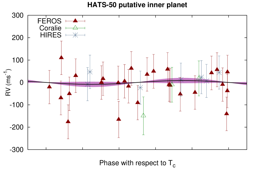
Figure 11: Phased high-precision RV measurements for HATS-50, after subtracting the orbital variation due to the confirmed transiting hot Jupiter, HATS-50b, and phase-folded at the period (0.77 days) of the candidate inner transiting planet, HATS-50c. The line shows the best-fit circular orbit at this period, while the shaded region shows the 1-sigma uncertainty bounds on this model. The instruments used are labelled in the plots.

4 Summary and discussion

Figure 12: Mass-period diagram of all known transiting hot Jupiters, i.e. transiting exoplanets in the mass range $0.3\,M_{\rm J}<M_{\rm p}<5\,M_{\rm J}$ and with an orbital period less than 10 days. The planets are represented by circles, whose size is proportional to their radius. Color indicates equilibrium temperature. The positions of HATS-50b, HATS-51b, HATS-52b, HATS-53b are highlighted with green boxes. The error bars have been suppressed for clarity. Data taken from the Transiting Extrasolar Planet Catalogue (TEPCat).

Figure 13: The masses and radii of the known transiting extrasolar planets. The plot is restricted to exoplanets with values of the mass until $2.5\,M_{\rm J}$ and radius until $2.0\,R_{\rm J}$. Grey points denote values taken from TEPCat. Their error bars have been suppressed for clarity. The new HATS exoplanets, HATS-50b, HATS-51b, HATS-52b and HATS-53b, are shown in red points with error bars. Dotted lines show where density is 2.5, 1.0, 0.5, 0.25 and 0.1 $\rho_{\rm J}$.

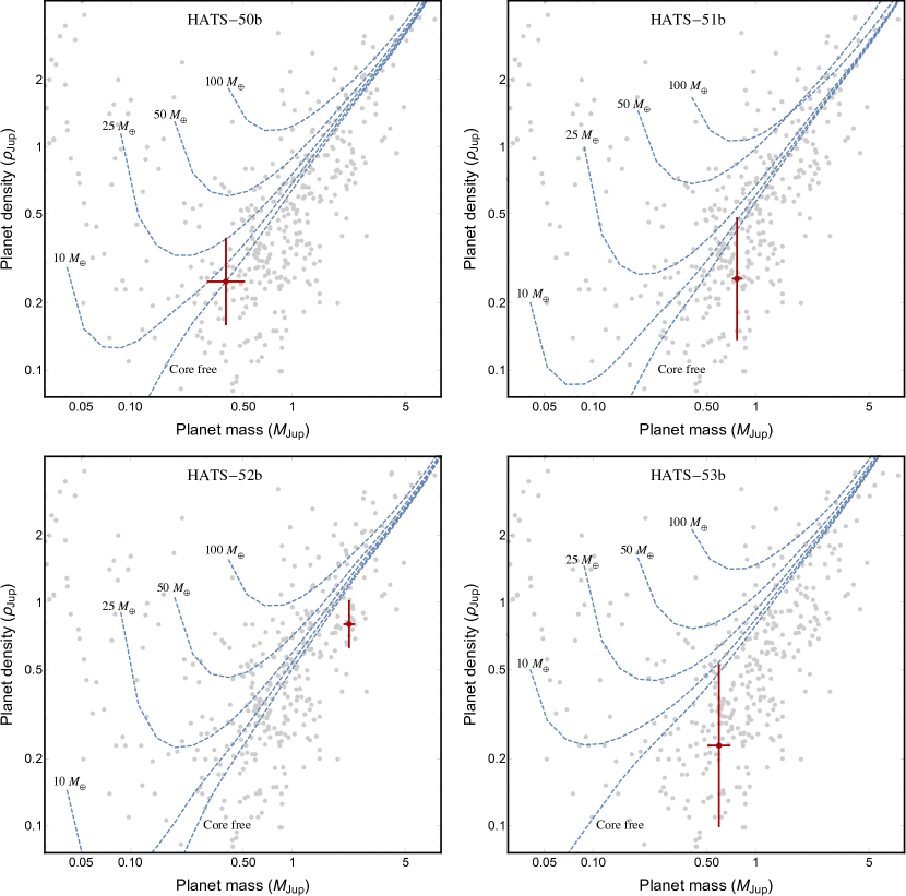
Figure 14: The mass-density diagram of the currently known transiting exoplanets. The grey points denote values taken from TEPCat. Their error bars have been suppressed for clarity. The position of HATS-50b, HATS-51b, HATS-52b, HATS-53b are shown in red with error bars in the top-left, top-right, bottom-left and bottom-right panel, respectively. Four planetary models, with various heavy-element core masses (10, 25, 50, and 100 Earth mass) and another without a core (Fortney et al., 2007) are plotted for comparison. They were estimated for a planet at 0.045 au from a parent star with an age of 1.0 Gyr (top-left panel), 0.045 au and 3.16 Gyr (top-right panel), 0.02 au and 1.0 Gyr (bottom-left panel), and 0.045 au and 10 Gyr (bottom-right panel).

Having now exceeded 50 discoveries, HATSouth turns out to be one of the most efficient ground-based survey for detecting transiting exoplanets. Thanks to systematic photometric observations of southern-sky regions with the HATSouth robotic telescopes, we have presented the discovery of four new hot Jupiters, namely HATS-50b, HATS-51b, HATS-52b and HATS-53b. After their detection with the survey facilities, their planetary nature was robustly confirmed through photometric follow-up observations, and extensive RV measurements, as described in the previous sections.

All the photometric and spectroscopic data that we have collected were used for fully characterizing these new exoplanetary systems. From the analysis of the parents stars we found that they are G-type main-sequence stars and have very different ages. While HATS-50 and HATS-52 are young ($\approx 1.2$ Gyr), HATS-51 has an age similar to the Sun ($\approx 4.7$ Gyr), and HATS-51 appears to be very old ($\approx 9.0$ Gyr). Three of them resulted to be metal rich (HATS-50: $\rm[Fe/H]=0.300\pm 0.056$; HATS-51: $\rm[Fe/H]=0.300\pm 0.030$; HATS-52: $\rm[Fe/H]=0.22\pm 0.10$;), whereas HATS-53 presents a metal abundance similar to the Sun, $\rm[Fe/H]=0.010\pm 0.066$.

Figure 12 shows the positions of the four new HATS planets in the current planet period-mass diagram. They are plotted together with all the other known transiting hot Jupiters, i.e. exoplanets having a mass in the range $0.3\,M_{\rm J}<M_{\rm p}<5\,M_{\rm J}$ and an orbital period less than 10 days (data taken from the TEPCat catalogue on October 30, 2017). While HATS-51b and HATS-53b have a similar Safranov number (see Table 6) and are located in regions of the diagram where the hot Jupiters are very packed, HATS-50b and HATS-52b are in less-populated regions of the diagram, highlighting the well-known desert of low-mass Jupiters and Neptunes at low orbital periods (e.g. Mazeh et al., 2005; Benítez-Llambay et al., 2011; Mazeh et al., 2016).

The inflated size of HATS-50b, HATS-51b and HATS-53b is evident from Figure 13, in which the mass-radius diagram of known transiting exoplanets (with mass and radius up to $2.5\,M_{\rm J}$ and $2.0\,R_{\rm J}$, respectively) is shown. The three planets exhibit a similar density. Instead, due to its mass, HATS-52b occupies a zone a slightly apart from the other three and from the crowd of giant exoplanets, similar to the physical characteristics of WASP-36b (Mancini et al., 2016) and Kepler-17b (Désert et al., 2011). Moreover, since the stellar radiation that it receives from its star is $\approx 2.6\times 10^{9}$ erg sec^-1, HATS-52b is very hot ($T_{\rm eq}=1834\pm 73$ K) and belongs to the pM class of hot Jupiters, according to the terminology of Fortney et al. (2008).

The panels of Figure 14 show the position of the four planets in the mass-density diagram of the currently known transiting exoplanets. Each planet is compared with five different theoretical models estimated by Fortney et al. (2007). Each model has a different core of heavy-elements, i.e. 0, 10, 25, 50, and 100 Earth mass and each panel shows models that were estimated for different values of planet-star separation and stellar age, as explained in the caption of the figure. The four planets have densities comparable with models of core-free planets. One pontential explanation could be that the planets are bloated which would provide the incorrect impression of a too small core mass (Thorngren & Fortney, 2017). An alternative explanation would be that relatively low opacities would allow gas runaway accretion also for lower core masses (Mordasini, 2014; Ormel, 2014). In a recent investigation based on results of the Juno mission the core mass of Jupiter was estimated to be in the range between $7-25$ Earth mass (Wahl et al., 2017) which points to a relatively small core mass.

Finally, we would like to remark the possible existence of an inner planet in the HATS-50 planetary system. The analysis of the photometric data of the HATSouth survey has actually revealed a small transit signal with duration of 46 minutes (see Fig. 2), yet with a SDE below our threshold for selecting it as a planet candidate. The radius, estimated from the best-fitting model of the HATS photometry and the upper limit of its mass, as coming from the RV measurements, suggest that this putative planet c has physical characteristics of a super Neptune. Its short periodicity (0.77 days) place it in the Neptune desert, thus making it an interesting candidate to possibly confirm or invalidate with more performing astronomical facilities, as the next space telescope TESS will be.

References

- Addison et al. (2013) Addison, B. C., Tinney, C. G., Wright, D. J., et al. 2013, ApJ, 774, L9
- Alsubai et al. (2013) Alsubai, K. A., Parley, N. R., Bramich, D. M., et al. 2013, Acta Astron., 63, 465
- Bakos et al. (2004) Bakos, G. Á., Noyes, R. W., Kovács, G. et al. 2004, PASP, 116, 266
- Bakos et al. (2010) Bakos, G. Á., Torres, G., Pál, A., et al. 2010, ApJ, 710, 1724
- Bakos et al. (2013) Bakos, G. Á., Csubry, Z., Penev, K., et al. 2013, PASP, 125, 154
- Bakos et al. (2015) Bakos, G. Á., Penev, K., Bayliss, D., et al. 2015, ApJ, 813, 111
- Batygin et al. (2016) Batygin, K., Bodenheimer, P. H., Laughlin, G. P. 2016, ApJ, 829, 114
- Bayliss et al. (2013) Bayliss, D., Zhou, G. and Penev, K., et al. 2013, AJ, 146, 113
- Bayliss et al. (2015) Bayliss, D., Hartman, J. D., Bakos, G. Á., et al. 2015, AJ, 150, 49
- Becker et al. (2015) Becker, J. C., Vanderburg, A., Adams, F. C., Rappaport, S. A., Schwengeler, H. M. 2015, ApJ, 812, L18
- Benítez-Llambay et al. (2011) Benítez-Llambay, P. and Masset, F. and Beaugé, C. 2011, A&A, 528, A2
- Berta-Thompson et al. (2015) Berta-Thompson, Z. K., Irwin, J., Charbonneau, D., et al. 2015, Nature, 527, 204
- Bitsch & Kley (2011) Bitsch, B., Kley, W. 2011, A&A, 530, A41
- Bodenheimer et al. (2000) Bodenheimer, P. and Hubickyj, O. and Lissauer, J. J. 2000, Icarus, 143, 2
- Boley et al. (2016) Boley, A. C., Granados Contreras, A. P., Gladman, B. 2016, ApJ, 817, L17
- Borucki et al. (2011) Borucki, W. J., Koch, D. G., Basri, G., et al. 2011, ApJ, 736, 19
- Brahm et al. (2016) Brahm, R. and Jordán, A. and Bakos, G. Á. et al. 2016, AJ, 151, 89
- Brahm et al. (2017a) Brahm, R., Jordán, A., Hartman, J., & Bakos, G. 2017, MNRAS, 467, 971
- Brahm et al. (2017b) Brahm, R., Jordán, A., Espinoza, N. 2017, PASP, 129, 034002
- Brown et al. (2013) Brown, T. M., Baliber, N., Bianco, F. B., et al. 2013, PASP, 125, 1031
- Burke et al. (2007) Burke, C. J., McCullough, P. R., Valenti, J. A., et al. 2007, ApJ, 671, 2115
- Cardelli et al. (1989) Cardelli, J. A., Clayton, G. C., & Mathis, J. S. 1989, ApJ, 345, 245
- Charbonneau et al. (2009) Charbonneau, D., Berta, Z. K., Irwin, J. et al. 2009, Nature, 462, 891
- Chatterjee et al. (2008) Chatterjee, S., Ford, E. B., Matsumura, S., Rasio, F. A. 2008, ApJ, 686, 580
- Claret (2004) Claret, A. 2004, A&A, 428, 1001
- Damasso et al. (2015) Damasso, M., Biazzo, K., Bonomo, A. S., et al. 2015, A&A, 575, A111
- Désert et al. (2011) Désert, J.-M., Charbonneau, D., Demory, B.-O., et al. 2011, ApJS, 197, 14
- Desidera et al. (2014) Desidera, S. and Bonomo, A. S. and Claudi, R. U., et al. 2014, A&A, 567, L6
- Dopita et al. (2007) Dopita, M., Hart, J., McGregor, P., et al. 2007, Ap&SS, 310, 255
- Dressing & Charbonneau (2013) Dressing, C. D., Charbonneau, D. 2013, ApJ, 767, 95
- Espinoza et al. (2016) Espinoza, N., Bayliss, D., Hartman, J. D., et al. 2016, AJ, 152, 108
- Fabrycky & Tremaine (2007) Fabrycky, D., Tremaine, S. 2007, ApJ, 669, 1298
- Fortney et al. (2007) Fortney, J. J., Marley, M. S., Barnes, J. W. 2007, ApJ, 659, 1661
- Fortney et al. (2008) Fortney, J. J., Lodders, K., Marley, M. S. 2008, ApJ, 678, 1419
- Fressin et al. (2013) Fressin, F., Torres, G., Charbonneau, D., et al. 2013, ApJ, 766, 81
- Gillon et al. (2016) Gillon, M., Jehin, E., Lederer, S. M., et al. 2016, Nature, 533, 221
- Girardi et al. (2000) Girardi, L., Bressan, A., Bertelli, G., & Chiosi, C. 2000, A&AS, 141, 371
- Gaudi et al. (2017) Gaudi, B. S. and Stassun, K. G. and Collins, K. A., et al. 2017, Nature, 546, 514
- Hansen & Barman (2007) Hansen, B. M. S., & Barman, T. 2007, ApJ, 671, 861
- Hartman et al. (2012) Hartman, J. D., Bakos, G. Á., Béky, B., et al. 2012, AJ, 144, 139
- Hartman et al. (2015) Hartman, J. D., Bayliss, D., Brahm, R., et al. 2015, 149, 166
- Hebb et al. (2009) Hebb, L., Collier-Cameron, A., Loeillet, B., et al. 2009, ApJ, 693, 1920
- Hellier et al. (2012) Hellier, C., Anderson, D. R., Collier Cameron, A. et al. 2012, MNRAS, 426, 739
- Henden et al. (2009) Henden, A. A., Welch, D. L., Terrell, D., Levine, S. E. 2009, American Astronomical Society Meeting Abstracts, 214, #407.02
- Hippler et al. (2009) Hippler, S., Bergfors, C., Brandner Wolfgang, et al. 2009, The Messenger, 137, 14
- Howard et al. (2010) Howard, A. W., Johnson, J. A., Marcy, G. W., et al. 2010, ApJ, 721, 1467
- Janson et al. (2017) Janson, M., Durkan, S., Hippler, S., et al. 2017, A&A, 599, A70
- Jordán et al. (2014) Jordán, A. and Brahm, R. and Bakos, G. Á., et al. 2014, AJ, 148, 29
- Kaufer & Pasquini (1998) Kaufer, A., & Pasquini, L. 1998, Proc. SPIE, 3355, 844
- Kovács et al. (2005) Kovács, G., Bakos, G., & Noyes, R. W. 2005, MNRAS, 356, 557
- Kovács et al. (2002) Kovács, G., Zucker, S., & Mazeh, T. 2002, A&A, 391, 369
- Lin et al. (1996) Lin, D. N. C., Bodenheimer, P., Richardson, D. C. 1996, Nature, 380, 606
- Linegren et al. (2016) Lindegren, L., Lammers, U., Bastian, U. et al. 2016, A&A, 595, A4
- Mancini et al. (2016) Mancini, L., Kemmer, J., Southworth, J., et al. 2016, MNRAS, 459, 1393
- Mandel & Agol (2002) Mandel, K., & Agol, E. 2002, ApJ, 580, L171
- Marzari & Nelson (2009) Marzari, F., Nelson, A. F. 2009, ApJ, 705, 1575
- Mayor et al. (2003) Mayor, M., Pepe, F., Queloz, D., et al. 2003, The Messenger, 114, 20
- Mazeh et al. (2005) Mazeh, T., Zucker, S., Pont, F. 2005, MNRAS, 356, 955
- Mazeh et al. (2016) Mazeh, T., Holczer, T., Faigler, S. 2016, A&A, 589, A75
- Mohler-Fischer et al. (2013) Mohler-Fischer, M. and Mancini, L. and Hartman, J. D., et al. 2003, A&A, 558, A55
- Mordasini (2014) Mordasini, C. 2014, A&A, 572, A118
- Ormel (2014) Ormel, C. W. 2014, ApJ, 789, L18
- Pál et al. (2008) Pál, A., Bakos, G. Á., Torres, G., et al. 2008, ApJ, 680, 1450
- Penev et al. (2013) Penev, K., Bakos, G. Á., Bayliss, D., et al. 2013, AJ, 145, 5
- Penev et al. (2016) Penev, K. and Hartman, J. D. and Bakos, G. Á. et al. 2016, AJ, 152, 127
- Pepper et al. (2007) Pepper, J., Pogge, R. W., DePoy, D. L., et al. 2007, PASP, 119, 923
- Pepper et al. (2012) Pepper, J., Kuhn, R. B., Siverd, R., et al. 2012, PASP, 124, 230
- Pollacco et al. (2006) Pollacco, D. L., Skillen, I., Collier Cameron, A., et al. 2006, PASP, 118, 1407
- Queloz et al. (2001) Queloz, D., Mayor, M., Udry, S., et al. 2001, The Messenger, 105, 1
- Rasio & Ford (1996) Rasio, F. A., Ford, E. B. 1996, Science, 274, 954
- Ricker et al. (2017) Ricker, G. R., & TESS Science Team 2017, American Astronomical Society Meeting Abstracts, 229, 104.09
- Sedaghati et al. (2017) Sedaghati, E., Boffin, H. M. J., MacDonald, R. J., et al. 2017, Nature, 549, 238
- Sing et al. (2016) Sing, D. K., Fortney, J. J., Nikolov, N., et al. 2016, Nature, 529, 59
- Sozzetti et al. (2007) Sozzetti, A., Torres, G., Charbonneau, D., et al. 2007, ApJ, 664, 1190
- Southworth (2011) Southworth, J. 2011, MNRAS, 417, 2166
- Thorngren & Fortney (2017) Thorngren, D. P., Fortney, J. J. 2017, submitted to AJ, arXiv:1709.04539
- Vogt et al. (1994) Vogt, S. S., Allen, S. L., Bigelow, B. C., et al. 1994, Proc. SPIE, 2198, 362
- Wahl et al. (2017) Wahl, S. M., Hubbard, W. B., Militzer, B., et al. 2017, Geophys. Res. Lett., 44, 4649
- Wheatley et al. (2017) Wheatley, P. J., West, R. G., Goad, M. R., et al. 2017, MNRAS accepted, arXiv:1710.11100
- Weinberg et al. (2013) Weinberg, M. D., Yoon, I., & Katz, N. 2013, ArXiv e-prints, arXiv:1301.3156
- Yi et al. (2001) Yi, S., Demarque, P., Kim, Y.-C., et al. 2001, ApJS, 136, 417
- Zacharias et al. (2012) Zacharias, N., Finch, C. T., Girard, T. M., et al. 2012, VizieR Online Data Catalog, 1322, 0
- Zechmeister & Kürster (2009) Zechmeister, M., & Kürster, M. 2009, A&A, 496, 577
- Zhou et al. (2014) Zhou, G., Bayliss, D., Hartman, J. D., et al. 2014, MNRAS, 437, 2831
- Zhou et al. (2015) Zhou, G., Bayliss, D., Hartman, J. D., et al. 2015, MNRAS, 451, 2263