Cosmic acceleration from a single fluid description

Abstract

We here propose a new class of barotropic factor for matter, motivated by properties of isotropic deformations of crystalline solids. Our approach is dubbed Anton-Schmidt’s equation of state and provides a non-vanishing, albeit small, pressure term for matter. The corresponding pressure is thus proportional to the logarithm of universe’s volume, i.e. to the density itself since $V\propto\rho^{-1}$. In the context of solid state physics, we demonstrate that by only invoking standard matter with such a property, we are able to frame the universe speed up in a suitable way, without invoking a dark energy term by hand. Our model extends a recent class of dark energy paradigms named logotropic dark fluids and depends upon two free parameters, namely $n$ and $B$. Within the Debye approximation, we find that $n$ and $B$ are related to the Grüneisen parameter and the bulk modulus of crystals. We thus show the main differences between our model and the logotropic scenario, and we highlight the most relevant properties of our new equation of state on the background cosmology. Discussions on both kinematics and dynamics of our new model have been presented. We demonstrate that the $\Lambda$CDM model is inside our approach, as limiting case. Comparisons with CPL parametrization have been also reported in the text. Finally, a Monte Carlo analysis on the most recent low-redshift cosmological data allowed us to place constraints on $n$ and $B$. In particular, we found $n=-0.147^{+0.113}_{-0.107}$ and $B=3.54\times 10^{-3}$.

I Introduction

In the context of homogeneous and isotropic universe, Einstein’s gravity supplies a cosmological description which commonly makes use of a perfect fluid energy momentum tensor, with barotropic equation of state given by the ratio between pressure and density uno1 ; uno2 . Observations have shown that under this hypothesis a negative anti-gravitational equation of state is requested to speed up the universe at our times supernovae ; Suzuki11 . Several scenarios have been introduced in the literature with the aim of describing the cosmic acceleration in terms of exotic fluids which counterbalance the action of gravity due1 ; due2 . The simplest approach is offered by a quantum vacuum energy density given by the cosmological constant $\Lambda$ costante . One of the advantages of $\Lambda$ is to provide a constant equation of state, i.e. $w=-1$, with constant pressure and density. Although attractive, the corresponding paradigm, named the $\Lambda$CDM model, is jeopardized by some caveats which may limit its use. Dark energy is the simplest class of extensions of the concordance model. Even though a wide number of dark energy models has been introduced Copeland06 ; Bamba12 , the problem of the onset and nature of cosmic acceleration remains an open challenge of modern cosmology altro1 .

Among all approaches, modifying the fluid responsible for the cosmic acceleration is likely the simplest way to account for the dark energy properties at large scales. A relevant example has been offered by Chaplygin gas chap1 and extensions which are built up with different equations of state chap2 . Since the cosmic pressure is negative, we wonder whether matter alone can be used to provide, at certain stages of universe’s evolution, a negative pressure altro2 . To do so, we analyze in nature possible cases in which this may happen. One possibility is to consider standard matter with a different equation of state compared to the usual case in which its pressure vanishes. The process that enables matter to pass from a pressureless equation of state to a negative pressure is due to the cosmic expansion as the standard model provides.

We thus follow this strategy and we propose matter obeying the Anton-Schmidt’s equation of state within the Debye approximation AntonSchmidt . The aforementioned framework has been introduced to empirically describe the pressure of crystalline solids which deform under isotropic stress (for a review, see bis ). If one considers the universe to deform under the action of cosmic expansion, it would be possible to model the fluid by means of such an equation of state that turns out to be naturally negative bis2 .

In this paper, we apply the properties of Anton-Schmidt’s equation of state in the framework of Friedmann-Robertson-Walker (FRW) universe. We first motivate the choice of Anton-Schmidt’s equation of state. Afterwards, we show the technique to pass from pressureless matter to Anton-Schmidt dark energy scenario. Here, we show that if matter obeyed the Anton-Schmidt’s equation of state, it would be possible to fuel the universe to accelerate without the need of the cosmological constant, i.e. $\Lambda$. To figure this out, we highlight that dark energy becomes a consequence of Anton-Schmidt’s equation of state in which matter naturally provides a negative barotropic factor. This unusual behaviour for matter is the basic demand to get speed up after the transition redshift. We analyze different epochs, i.e. at late-times and before current era, and we identify the mechanism responsible for the cosmic acceleration. We investigate some properties of our model and we show that it depends upon two parameters only, characterized by precise physical meanings. The key feature lies on analyzing the role played by universe’s volume which influences the equation of state itself. In particular, a negative value for pressure becomes dominant as the volume of the universe overcomes a certain value. We thus show that although the model drives the universe dynamics at all stages, relevant consequences raise only as the volume takes a given value, enabling the pressure not to be negligible. In this scenario, we notice our model matches the approach of logotropic dark energy (LDE) model Chavanis15 . We thus propose a common origin between Anton-Schmidt dark energy and LDE. To do so, we investigate the limits to LDE and we show in which regimes our scenario becomes equivalent, emphasizing the main differences between the two approaches. To consolidate our theoretical alternative to $\Lambda$, we finally compute observational constraints at the level of background cosmology using supernova data, differential Hubble rate and baryon acoustic oscillation measurements. We thus perform a combined fit providing numerical bounds over our free parameters by means of Monte Carlo analysis.

The paper is structured as follows. In Sec. II, we describe the Anton-Schmidt scenario for crystalline solids in the Debye approximation. We also emphasize the role played by $V_{0}$, as scaling volume inside the pressure definition. Afterwards, in the same section we discuss the technique able to split the whole energy density into two parts, corresponding to a pressureless term and a pushing up effective dark energy counterpart. In Sec. III, we thus describe how acceleration born from our framework, highlighting implications in modern cosmology and then comparing our outcomes with the concordance and the Chevallier-Polarski-Linder parametrization. We then report the onset of cosmic acceleration and the role played by the sound speed. In Sec. IV, we describe observational constraints over our model, which lie on the Monte Carlo techniques based on affine-invariant ensemble sampler. We conclude our work with conclusions and perspectives summarized in Sec. V.

II Anton-Schmidt’s matter fluid as effective dark energy

The issue of negative pressure jeopardizes the cosmological standard model, since it is not easy to get evidences of negative pressure in laboratory. However, in the framework of condensed matter and solid state physics it could happen that effective pressures become locally negative. Some other cases permit scenarios in which the physical counterpart of the pressure is effectively negative. This is the case of the Anton-Schmidt’s equation of state for crystalline solids AntonSchmidt . In particular, the Anton-Schmidt’s equation of state gives the empirical expression of crystalline solid’s pressure under isotropic deformation. In the Debye approximation, one can write the Anton-Schmidt’s pressure as follows:

$$P(V)=-\beta\left(\dfrac{V}{V_{0}}\right)^{-\frac{1}{6}-\gamma_{G}}\ln\left(\dfrac{V}{V_{0}}\right)\,,$$ (1)

where

• $V$ is the volume of the crystal, and $V_{0}$ is the equilibrium volume. In particular, $V_{0}$ shows the limit at which the pressure vanishes. This occurrence is found as $V=V_{0}$, enabling $V_{0}$ to be considered as a barrier which shifts among different signs of $P$. In fact, as $V<V_{0}$ the pressure is positive, for positive bulk modulus, while negative in the opposite case, i.e. $V_{0}<V$. For negative bulk modulus, the cases are reversed, although negative $\beta$ are here excluded since apparently not significant in our analyses;

• $\beta$ is the bulk modulus at $V_{0}$. This quantity is intimately related to sound perturbations and elasticity in fluids. In such a picture, $\beta$ is in analogy with the spring constant of an oscillator, once given a fluid or a crystal. It may be viewed as a heuristic measurement of how much physical dimensions, i.e. volume, lengths, change under the action of external forces. In our case, we take the standard definition of $\beta$ and we assume it is related to the variation of $P$ in terms of the volume by

  $$\beta=-V_{0}\left(\dfrac{dP}{dV}\right)_{V=V_{0}}\ ;$$ (2)

• $\gamma_{G}$ is the dimensionless Grüneisen parameter Gruneisen12 , which has both a thermal and an equivalent microscopic interpretation. The macroscopic definition is related to the thermodynamic properties of the material:

  $$\gamma_{G}=\frac{\alpha VK_{T}}{C_{V}}\ ,$$ (3)

  where $\alpha$ is the thermal coefficient, $K_{T}$ is the isothermal bulk modulus, and $C_{V}$ is the heat capacity at constant volume. The microscopic formulation accounts for the variation of the vibrational frequencies of the atoms in the solid with $V$. In fact, the Grüneisen parameter of an individual vibrational mode $i$ is given by

  $$\gamma_{i}=-\dfrac{d\ln\omega_{i}}{d\ln V}\ ,$$ (4)

  where $\omega_{i}$ is the vibrational frequency of the $i$th mode. Under the quasi-harmonic approximation, it is possible to relate the macroscopic definition of $\gamma_{G}$ to its microscopic definition if one writes Barron57

  $$\gamma_{G}=\dfrac{1}{C_{V}}\sum_{i}C_{V,i}\gamma_{i}=\dfrac{\alpha VK_{T}}{C_{V}}\ ,$$ (5)

  where $C_{V,i}$ is the contribution of each mode to the heat capacity. In the Debye model, the Grüneisen parameter reads

  $$\gamma_{G}=\dfrac{d\ln\theta_{D}}{d\ln V}\ ,$$ (6)

  where $\theta_{D}$ is the Debye temperature Debye defined as $\theta_{D}=\hbar\omega_{D}/k_{B}$, where $\hbar$ and $k_{B}$ are the Planck’s and Boltzmann’s constants, respectively, and $\omega_{D}$ is the maximum vibrational frequency of a solid’s atoms. The values of the Grüneisen parameter do not show big variations for a wide variety of chrystals Anderson89 and are typically in the range 1 to 2.

As a consequence of our recipe, under the hypothesis of Anton-Schmidt fluid, we immediately find that:

1. the whole universe may be modelled by a single dark counterpart under the form of Anton-Schmidt fluid. In particular, one can consider that matter fuels the cosmic speed up, if its equation of state is supposed to be the one of Eq. 1;

2. admitting that matter depends on Anton-Schmidt’s equation of state means that $P\neq 0$ for matter. So the form of matter distribution in the whole universe is not exactly zero;

3. assuming for matter that $P\neq 0$, under the form of Eq. 1, is equivalent to employ a non-vanishing equation of state for matter, but small enough to accelerate the universe with a negative sign;

4. the sign of Anton-Schmidt’s equation of state for matter is naturally negative, by construction of the pressure itself;

5. the parameter $\gamma_{G}$ is not arbitrary and depends on the kind of fluid entering the energy momentum tensor. In the case of matter, in the homogeneous and isotropic universe, $\gamma_{G}$ will be a free parameter of the theory itself.

In our case, since we only have matter obeying Eq. 1, to guarantee the cosmic speed up at late times, one needs to overcome the limit:

$$\gamma_{G}=-\frac{1}{6}\,.$$ (7)

If $\gamma_{G}>-\frac{1}{6}$ the cosmic acceleration does not occur at $z\simeq 0$. In all cases the advantages of employing a matter term evolving as Eq. 1 are:

• the pressure is not postulated to be negative a priori as in the standard cosmological model. Notice that in the $\Lambda$CDM case one has at least two fluids: the first concerning pressureless matter, whereas the second composed by $\Lambda$. In such a picture, what pushes up the universe to accelerate is the cosmological constant. In our puzzle, neglecting all small contributions, such as neutrinos, radiations, spatial curvature, etc., one finds that standard matter is enough to enable the acceleration once Eq. (1) is accounted;

• the physical mechanism behind Eq. (1) states that if the universe expands then the net equation of state provides different behaviours, corresponding to deceleration at certain times and acceleration during other epochs;

• it is possible to measure in a laboratory the effects of Eq. 1, which is physical and does not represent a ad hoc construction of the universe pressure.

It is natural to suppose that Eq. 1 bids to the following limits:

$$\left\{\begin{array}[]{ll}\lim_{V\gg V_{0}}\,\,\Big{|}P(V)\Big{|}=\infty,&\hbox{$\gamma_{G}<-\dfrac{1}{6}$;}\\ \\ \lim_{V\ll V_{0}}\,\,\Big{|}P(V)\Big{|}=0\,,&\hbox{$\gamma_{G}<-\dfrac{1}{6}$.}\end{array}\right.$$

Thus, there exists a volume at which the matter pressure turns out to be dominant over the case $P=0$. It follows that matter with the above pressure can accelerate the universe after a precise time. This is a consequence of our model and it is not put by hand as in the concordance paradigm.

Indeed, introducing two fluids: matter and $\Lambda$ there exists a time at which $\Lambda$ dominates over matter and pushes up the universe. In our approach, there exists one fluid, with a single equation of state, able to accelerate the universe as the volume passes the barrier $V\simeq V_{0}$. This means that the transition redshift is not actually relevant, because having one fluid only, the whole universe dynamics is essentially dominated by the fluid dynamics itself.

We can focus on three different cases, reported below.

case 1

The time before passing the $V_{0}$ barrier, i.e. $V<V_{0}$. In such a case, there exists an expected matter dominated phase. Indeed, when $V<V_{0}$, one gets the limit above stated which provides exactly the pressureless case $P=0$, as in the standard model paradigm.

case 2

the time of equivalence between $V$ and the $V_{0}$ barrier, i.e. $V=V_{0}$. In this case, we lie on the transition time, which occurs as $V=V_{0}$. In this case there exists a transition at a transition time, which leads to $V(z_{tr})=V_{0}$.

case 3

the time after passing the $V_{0}$ barrier. Here, since $V>V_{0}$ one passes from $P=0$ to $P<0$ and matter starts to accelerate the universe instead of decelerating it.

Following the notation introduced in the context of the LDE model Chavanis15 , we express the volume in terms of mass density, $V\propto\rho^{-1}$, and recast Eq. 1 as

$$P(\rho)=A\left(\dfrac{\rho}{\rho_{*}}\right)^{-n}\ln\left(\dfrac{\rho}{\rho_{*}}\right)\ ,$$ (10)

where $\rho_{*}$ is a reference density. The new notation implies $A\propto\beta$ and $n=-\frac{1}{6}-\gamma_{G}$. For $n=0$, Eq. 10 reduces to the equation of state characteristic of the logotropic cosmological models Chavanis15 , in which the constant $A$ represents the logotropic temperature, positive-definite.

In the present work we want to study the dynamical evolution of a universe made of a single fluid described by the Anton-Schmidt’s equation of state. We assume homogeneity and isotropy on large scales Peebles93 and, in agreement with the Cosmic Microwave Background (CMB) observations Planck15 , we consider a flat universe. Then, the Friedmann equation is given by

$$\left(\dfrac{\dot{a}}{a}\right)^{2}=\dfrac{8\pi G}{3c^{2}}\epsilon\ ,$$ (11)

where the ‘dot’ indicates derivative with respect to the cosmic time $t$, and $a(t)$ is the scale factor normalized to unity today $(a_{0}=1)$ To determine the total energy density $\epsilon$, we assume an adiabatic evolution for the fluid, so that the first law of thermodynamics reads

$$d\epsilon=\left(\dfrac{\epsilon+P}{\rho}\right)d\rho\ .$$ (12)

For $P(\rho)$ as given in Eq. 10, the above equation can be integrated and one obtains

$$\epsilon =\rho c^{2}+\rho\int^{\rho}d\rho^{\prime}\ \dfrac{p(\rho^{\prime})}{\rho^{\prime 2}}$$ (13)

$$=\rho c^{2}-\left[\dfrac{A}{n+1}\left(\dfrac{\rho}{\rho_{*}}\right)^{-n}\ln\left(\dfrac{\rho}{\rho_{*}}\right)+\dfrac{A}{(n+1)^{2}}\left(\dfrac{\rho}{\rho_{*}}\right)^{-n}\right],$$

for $n\neq-1$. Eq. 13 tells us that the energy density of the fluid is the sum of its rest-mass energy ($\rho c^{2}$) and its internal energy. The first term, describing a pressureless fluid, mimics matter, while the second term, which arises from pressure effects, can be interpreted as the dark energy term. Hence, this approach intends to unify dark matter and dark energy into a single dark fluid. Nonetheless, to draw a parallel with the standard scenario in which matter and dark energy are expressions of two separate fluids, we decide to write Eq. 13 as

$$\epsilon=\epsilon_{m}+\epsilon_{de}\,,$$ (14)

with

$$\epsilon_{m}=\rho c^{2}\ ,$$ (15)

$$\epsilon_{de}=-\dfrac{A}{n+1}\left(\dfrac{\rho}{\rho_{*}}\right)^{-n}\ln\left(\dfrac{\rho}{\rho_{*}}\right)-\dfrac{A}{(n+1)^{2}}\left(\dfrac{\rho}{\rho_{*}}\right)^{-n}.$$ (16)

In the early universe ($a\rightarrow 0$, $\rho\rightarrow\infty$), the rest-mass energy $\epsilon_{m}$ dominates. However, if $n<0$ the pressure given in Eq. 10 is not vanishing as expected in the standard matter-dominated universe. This is due to the fact that the Anton-Schmidt’s equation of state in the Debye approximation cannot describe the cosmic fluid of the early phase cosmology, when temperatures are much higher than the Debye temperatures of solids. In any case, if one wants to extend our model to early times would notice that $P\ll\epsilon$ for $\rho\rightarrow\infty$, and thus the fluid behaves as if it were pressureless, similarly to the case of the LDE model, as pointed out in Chavanis17 . At late times $(\rho\ll 1)$, the internal energy $\epsilon_{de}$ dominates and, for $n<0$, the pressure tends to a constant negative value as in a universe that is dominated by dark energy.

In the next section, we shall analyze the cosmological implications of such a picture at the background level. We compare the features of the model we propose with the standard cosmological scenarios, and we investigate the epoch of the dark energy dominance that drives the accelerated expansion of the universe.

III Consequences on background cosmology

The relation between the energy density and the scale factor for a given barotropic fluid is given by the continuity equation:

$$\dot{\epsilon}+3\dfrac{\dot{a}}{a}(\epsilon+P)=0\ .$$ (17)

Combining Eq. 12 and Eq. 17 yields

$$\dot{\rho}+3\dfrac{\dot{a}}{a}\rho=0\,,$$ (18)

which, once integrated, gives the evolution of the rest-mass density:

$$\rho=\dfrac{\rho_{m,0}}{a^{3}}\ .$$ (19)

Using Eqs. 19, 15 and 16, we get

$$\epsilon_{m}=\dfrac{\rho_{m,0}c^{2}}{a^{3}},$$ (20)

$$\epsilon_{de}=-\dfrac{A}{n+1}\left(\dfrac{\rho_{m,0}}{\rho_{*}a^{3}}\right)^{-n}\ln\left(\dfrac{\rho_{m,0}}{\rho_{*}a^{3}}\right)-\dfrac{A}{(n+1)^{2}}\left(\dfrac{\rho_{m,0}}{\rho_{*}a^{3}}\right)^{-n},$$ (21)

or equivalently,

$$\epsilon_{m}=\epsilon_{m,0}a^{-3},$$ (22)

$$\epsilon_{de}=\epsilon_{de,0}a^{3n}+\dfrac{3A}{n+1}\left(\dfrac{\rho_{m,0}}{\rho_{*}}\right)^{-n}a^{3n}\ln a,$$ (23)

where $\epsilon_{m,0}$ and $\epsilon_{de,0}$ are the energy densities evaluated at the present time. Introducing the Hubble parameter $H\equiv\dot{a}/a$ and the critical energy density $\epsilon_{c}\equiv 3H_{0}^{2}c^{2}/(8\pi G)$, Eq. 11 can be rewritten as

$$H^{2}=H_{0}^{2}\left(\dfrac{\epsilon_{m}}{\epsilon_{c}}+\dfrac{\epsilon_{de}}{\epsilon_{c}}\right),$$ (24)

where the energy density has been decomposed as in Eq. 14. One can define the normalized matter and dark energy densities,

$$\Omega_{m0} \equiv\dfrac{\epsilon_{m,0}}{\epsilon_{c}}\,,$$ (25a)

$$\Omega_{de,0} \equiv\dfrac{\epsilon_{de,0}}{\epsilon_{c}}\,,$$ (25b)

satisfying the condition $\Omega_{de,0}=1-\Omega_{m0}$. Thus, after simple manipulations, Eq. 24 becomes

$$H^{2}=H_{0}^{2}\left[\dfrac{\Omega_{m0}}{a^{3}}+(1-\Omega_{m0})(1+3B\ln a)a^{3n}\right]\,,$$ (26)

where, for convenience, we introduce

$$B=\dfrac{A}{n+1}\left(\dfrac{\rho_{m,0}}{\rho_{*}}\right)^{-n}\dfrac{1}{\epsilon_{c}\Omega_{de,0}}\ .$$ (27)

For $n=0$, Eq. 27 reduces to

$$B\big{|}_{n=0}=\dfrac{A}{\epsilon_{c}\Omega_{de,0}}\ ,$$ (28)

which represents the dimensionless logotropic temperature. To calculate the equation of state parameter $w=P/\epsilon$ in terms of the logotropic temperature, we rearrange Eqs. 10 and 14 as

$$P=-\epsilon_{c}(1-\Omega_{m0})\left[B+(n+1)(1+3B\ln a)\right]a^{3n},$$ (29)

$$\epsilon=\dfrac{\epsilon_{c}\Omega_{m0}}{a^{3}}+\epsilon_{c}(1-\Omega_{m0})(1+3B\ln a)a^{3n}\ .$$ (30)

Thus, one obtains

$$w=-\dfrac{(1-\Omega_{m0})\left[B+(n+1)(1+3B\ln a)\right]a^{3n}}{\Omega_{m0}a^{-3}+(1-\Omega_{m0})\left(1+3B\ln a\right)a^{3n}}\ .$$ (31)

Fixing the indicative value $\Omega_{m0}=0.3$, we show in Fig. 1 the behaviour of $P$ for different values of the parameters $B$ and $n$. Fig. 2 shows the evolution of the energy density in terms of the scale factor. For $B>0$, after reaching the minimum, the energy density increases with the scale factor characterizing a phantom universe. The behaviour of the equation of state parameter is shown in Fig. 3.

For $a\rightarrow\infty$, $w\rightarrow-1$. When $n=0$, the equation of state parameter reduces to

$$w\big{|}_{n=0}=-\dfrac{(1-\Omega_{m0})(B+1+3B\ln a)}{\Omega_{m0}a^{-3}+(1-\Omega_{m0})(1+3B\ln a)}\ ,$$ (32)

proper of the LDE model Chavanis15 .

Figure 1: Dynamical evolution of the pressure for different values of $B$ and $n=0$ (top), and for different values of $n$ and $B=0.1$ (bottom). The matter density parameter is fixed to $\Omega_{m0}=0.3$.

Figure 2: Dynamical evolution of the energy density for different values of $B$ and $n=0$ (top), and for different values of $n$ and $B=0.1$ (bottom). $\Omega_{m0}$ is kept fixed to the value of 0.3.

Figure 3: Dynamical evolution of the equation of state parameter for different values of $B$ and $n=0$ (top), and for different values of $B$ and $n=0$. In both plots, $\Omega_{m0}=0.3$. The black line separates the “normal” values from the phantom values $(w<-1)$.

We now focus our study on the dark energy equation of state parameter: $w_{de}=P_{de}/\epsilon_{de}$. Since the contribution of matter is negligible, one can simply identify the total pressure given in Eq. 29 with the dark energy pressure,

$$P_{de}=-\epsilon_{c}(1-\Omega_{m0})\left[B+(n+1)(1+3B\ln a)\right]a^{3n},$$ (33)

while the dark energy density term reads (cf. Eq. 30)

$$\epsilon_{de}=\epsilon_{c}(1-\Omega_{m0})(1+3B\ln a)a^{3n}\ .$$ (34)

Thus, one finally obtains

$$w_{de}=-(n+1)-\dfrac{B}{1+3B\ln a}\ .$$ (35)

III.1 Comparison with the concordance model

Our results contain the concordance paradigm. Hence, it is possible to recover the $\Lambda$CDM model from the Anton-Schmidt cosmological model. In fact, for $B=0$ and $n=0$, Eq. 26 reduces to

$$H^{2}=H_{0}^{2}\left(\dfrac{\Omega_{m0}}{a^{3}}+1-\Omega_{m0}\right)\,,$$ (36)

where $1-\Omega_{m0}=\Omega_{\Lambda}$ is the density parameter of the cosmological constant. In fact, in this limit the pressure Eq. 29 becomes a negative constant,

$$P=-\epsilon_{c}\Omega_{\Lambda}=-\epsilon_{\Lambda}\ ,$$ (37)

and the equation of state parameter Eq. 31 becomes

$$w=-\dfrac{1-\Omega_{m0}}{\Omega_{m0}a^{-3}+1-\Omega_{m0}}\ ,$$ (38)

whose present value is

$$w_{0}=-1+\Omega_{m0}\ .$$ (39)

As far as the dark energy equation of state is concerned, for $B=0$ and $n=0$, one has $w_{de}=-1$ (cf. Eq. 35) which corresponds to the cosmological constant case.

III.2 Comparison with the CPL model

A widely used parametrization for the dark energy equation of state is the Chevallier-Linder-Polarski (CPL) model Chevallier01 ; Linder03 , which describes a time-varying dark energy term:

$$w_{\text{CPL}}(a)=w_{0}+w_{a}(1-a)\ .$$ (40)

The above equation represents the first-order Taylor expansion around the present time and allows for deviations from the cosmological constant value $w_{0}=-1$. Moreover, this model well behaves from high redshifts ($w_{\text{CPL}}(0)=w_{0}+w_{a}$) to the present epoch ($w_{\text{CPL}}(1)=w_{0}$). It is possible to relate the constants $w_{0}$ and $w_{a}$ to the parameters $n$ and $B$. In fact, expanding Eq. 35 up to the first-order around $a=1$ yields

$$w_{de}\simeq-(1+n+B)-3B^{2}(1-a)\ ,$$ (41)

which, once compared with Eq. 40, gives

$$\left\{\begin{aligned} &w_{0}=-(1+n+B)\ ,\\ &w_{a}=-3B^{2}.\end{aligned}\right.$$ (42)

When $n=B=0$, we have $w_{0}=-1$ and $w_{a}=0$ as in the $\Lambda$CDM model.

III.3 The onset of cosmic acceleration

The rate of cosmic expansion is provided by the deceleration parameter Weinberg72 :

$$q\equiv-\dfrac{\ddot{a}a}{\dot{a}^{2}}=-\dfrac{\dot{H}}{H^{2}}-1\ .$$ (43)

Specifically, the universe is undergoing an accelerated expansion if $-1\leq q<0$. It is convenient to re-express Eq. 43 in terms of the derivative of the expansion rate with respect to the scale factor as

$$q=-\dfrac{a}{H}\dfrac{dH}{da}-1\ .$$ (44)

Plugging the expression of $H$ given by Eq. 26 into the above relation, one obtains

$$q=\dfrac{\Omega_{m0}a^{-3}-(1-\Omega_{m0})\left[3(n+B)+3B(3n+2)\ln a+2\right]a^{3n}}{2\left[\Omega_{m0}a^{-3}+(1-\Omega_{m0})(1+3B\ln a)a^{3n}\right]}$$ (45)

In Fig. 4 we show the analytical behaviour of $q$ as a function of the scale factor for different values of $B$ and $n$, while the matter density parameter is fixed to $\Omega_{m0}=0.3$.

Figure 4: Dynamical evolution of the deceleration parameter for different values of $B$ and $n=0$ (top), and for different values of $n$ and $B=0.1$ (bottom). The matter density is fixed to $\Omega_{m0}=0.3$. The black line separates the region of deceleration $(q>0)$ from the region of acceleration $(q<0)$. $q<-1$ indicates phantom universe.

For $n=0$, Eq. 45 reduces to

$$q\Big{|}_{n=0}=\dfrac{\Omega_{m0}a^{-3}-(1-\Omega_{m0})\left[3B+6B\ln a+2\right]}{2\left[\Omega_{m0}a^{-3}+(1-\Omega_{m0})(1+3B\ln a)\right]}\ ,$$ (46)

analogous to the LDE models and it converges to $q\rightarrow-1$ when $a\rightarrow\infty$, indicating a de-Sitter phase. In the limit $n=B=0$, we recover the deceleration parameter of the $\Lambda$CDM model:

$$q_{\Lambda\text{CDM}}=\dfrac{\Omega_{m0}a^{-3}-2(1-\Omega_{m0})}{2\left(\Omega_{m0}a^{-3}+1-\Omega_{m0}\right)}\ .$$ (47)

The point $a_{acc}$ at which the universe starts accelerating is found for $q=0$, which applied to Eq. 45 gives the condition

$$a^{-3(1+n)}=\dfrac{1-\Omega_{m0}}{\Omega_{m0}}\Big{[}3(n+B)+3B(3n+2)\ln a+2\Big{]}.$$ (48)

A straightforward solution is found for $n=-2/3$, for which the above condition reads

$$a_{acc}\Big{|}_{n=-\frac{2}{3}}=\dfrac{\Omega_{m0}}{3B(1-\Omega_{m0})}\ .$$ (49)

Further, we can find the condition to get an accelerated universe today. Evaluation of Eq. 45 at the present time yields

$$q_{0}=\dfrac{\Omega_{m0}-(1-\Omega_{m0})\left[3(n+B)+2\right]}{2}\ ,$$ (50)

and imposing $-1\leq q_{0}<0$, one obtains the required condition:

$$\dfrac{\Omega_{m0}-2/3}{1-\Omega_{m0}}<n+B\leq\dfrac{\Omega_{m0}}{1-\Omega_{m0}}\ .$$ (51)

The transition between the matter and the dark energy eras occurs when the energy densities of both species satisfy $\epsilon_{m}=\epsilon_{de}$. Using Eqs. 22 and 21, the above condition becomes

$$\Omega_{m0}\ a^{-3(n+1)}=(1-\Omega_{m0})(1+3B\ln a)\ .$$ (52)

To find the scale factor at the transition $a_{tr}$, we expand the right-hand side of Eq. 52 in Taylor series up to the first order around $a=1$,

$$(1-\Omega_{m0})(1+3B\ln a)\simeq(1-\Omega_{m0})(1+3B(a-1))\ ,$$ (53)

inserting it back into Eq. 52:

$$\left(\dfrac{\Omega_{m0}}{1-\Omega_{m0}}\right)a^{-3(n+1)}-3Ba\simeq 1+3B\ .$$ (54)

So, if $n=-2/3$, the solution to Eq. 54 is

$$a_{tr}\Big{|}_{n=-\frac{2}{3}}\simeq\dfrac{1+3B}{\frac{\Omega_{m0}}{1-\Omega_{m0}}-3B}\ .$$ (55)

The $\Lambda$CDM limit is thus recovered by setting $n=B=0$ in Eq. 52:

$$a_{tr}\Big{|}_{\Lambda\text{CDM}}={\left(\dfrac{1-\Omega_{m0}}{\Omega_{m0}}\right)}^{-1/3}.$$ (56)

III.4 Analyzing the sound speed

The sound speed plays a key role in theory of perturbations to explain the formation of structures in the universe perturbations . It determines the length above which gravitational instability overcomes the radiation pressure, and the perturbations grow. For an adiabatic fluid, the sound speed is given by

$$c_{s}^{2}\equiv\dfrac{\partial P}{\partial\rho}\ .$$ (57)

If $c_{s}$ is comparable to the speed of light, pressure prevents density contrasts to grow significantly, whereas in a matter-dominated universe ($c_{s}=0$) the gravitational instability on small scales occurs.

To calculate the sound speed in terms of the parameters $B$ and $n$, we convert the derivative with respect to the density into the derivative with respect to the scale factor according to

$$\dfrac{\partial\rho}{\partial a}=-\dfrac{3\epsilon_{c}\Omega_{m0}}{c^{2}}a^{-4}\ ,$$ (58)

where we have used Eqs. 19, 20 and 25a. Therefore, from Eq. 57 we obtain

$$c_{s}^{2} ={\left(\dfrac{\partial\rho}{\partial a}\right)}^{-1}\dfrac{\partial P}{\partial a}$$

$$=c^{2}\left(\dfrac{1-\Omega_{m0}}{\Omega_{m0}}\right)a^{3(n+1)}\Big{[}B(1+2n)$$

$$\hskip 85.35826pt+n(n+1)(1+3B\ln a)\Big{]}$$ (59)

which turns out to be real only if

$$B(1+2n)+n(n+1)(1+3B\ln a)\geq 0\ .$$ (60)

In the logotropic limit, Eq. 59 becomes

$$\dfrac{c_{s}^{2}}{c^{2}}\bigg{|}_{n=0}=\dfrac{B}{a^{3}}\left(\dfrac{1-\Omega_{m0}}{\Omega_{m0}}\right),$$ (61)

which requires $B\geq 0$ for the speed of sound to be real. For $n=B=0$, we have $c_{s}^{2}=0$ consistently with the $\Lambda$CDM model. The functional behaviour of the speed of sound for different values of $B$ is displayed on Fig. 5.

Figure 5: Speed of sound as a function of the scale factor for different values of the parameter $B$, while $n=0$.

IV Observational constraints and experimental limits

In this section, we place observational constraints on our model using the most recent low-redshift cosmological data. To do that, we rewrite the Hubble rate (see Eq. 26) in terms of the redshift $z=a^{-1}-1$ as

$$H(z)=H_{0}\sqrt{\Omega_{m0}(1+z)^{3}+\dfrac{1-\Omega_{m0}}{(1+z)^{3n}}\left[1-3B\ln(1+z)\right]}\ .$$ (62)

At this point, we need to interpret the meaning of the reference density $\rho_{*}$ in Eq. 10. The author in Chavanis15 identified $\rho_{*}$ with the Planck density $\rho_{P}$. The reason of this choice is that the logotropic equation of state applied to dark matter halos shows a constant surface density profile in agreement with observations Donato09 ; Saburova14 , providing a very small value of $B$. This implies that the ratio between $\rho_{*}$ and the dark energy density is huge, of the same order as the ratio between the vacuum energy associated to the Planck density and $\rho_{\Lambda}$, which is at the origin of the cosmological constant problem cosm const problem . Thus, we set $\rho_{*}=\rho_{P}$ and write

$$B=\dfrac{A}{n+1}\left(\dfrac{\rho_{m,0}}{\rho_{P}}\right)^{-n}\dfrac{1}{\epsilon_{de,0}}\ .$$ (63)

Since the present dark energy density is

$$\epsilon_{de,0}=-\dfrac{A}{n+1}\left(\dfrac{\rho_{m,0}}{\rho_{P}}\right)^{-n}\left[\ln\left(\dfrac{\rho_{m,0}}{\rho_{P}}\right)+\dfrac{1}{n+1}\right],$$ (64)

we soon find that Eq. 63 becomes

$$B=\dfrac{1}{\ln\left(\dfrac{\rho_{P}}{\rho_{m,0}}\right)-\dfrac{1}{n+1}}\ .$$ (65)

Recalling the expressions for the present matter and the Planck densities, one has

$$\dfrac{\rho_{P}}{\rho_{m,0}}=\dfrac{8\pi c^{5}}{3\hbar GH_{0}^{2}\Omega_{m0}}\ .$$ (66)

As a consequence, $B$ is no longer a free parameter of the model, but depends on the fitting parameters $\{H_{0},\Omega_{m0},n\}$ that fully determinate the Hubble rate given by Eq. 62. We stress that $B$ as expressed in Eq. 63 shows a weak dependence on the value of $n$, since the ratio (66) is very large. In particular, $B$ takes always small values tending to zero when $n$ approaches $-1$.

In the next section, we present the datasets we used to perform our numerical analysis.

IV.1 Supernovae Ia data

The largest dataset we consider in our analysis is the JLA sample of SNe Ia standard candles Betoule14 . This catalogue consists of 740 measurements in the redshift range $0<z<1.3$ and provides model-independent apparent magnitudes at correspondent redshift. The SNe with identical colour, shape and galactic environment are assumed to have on average the same intrinsic luminosity for all redshifts. Every SN is characterized by a theoretical distance modulus,

$$\mu_{th}(z)=25+5\log_{10}[d_{L}(z)]$$ (67)

where

$$d_{L}(z)=(1+z)\int_{0}^{z}\dfrac{c\ dz^{\prime}}{H(z^{\prime})}$$ (68)

is the luminosity distance in a flat universe. The distance modulus is modelled as follows:

$$\mu_{obs}=m_{B}-(M_{B}-\alpha X_{1}+\beta C)$$ (69)

where $(m_{B},X_{1},C)$ are the observed peak magnitude in the rest-frame B band, the time stretching of the light-curve and the supernova colour at maximum brightness, respectively. The absolute magnitude $M_{B}$ is defined based on the host stellar mass $M_{host}$ as

$$M_{B}=\begin{cases}M,&\text{if}\ M_{host}<10^{10}M_{Sun}\\ M+\Delta_{M},&\text{otherwise}\end{cases}$$ (70)

$M$, $\Delta_{M}$, $\alpha$ and $\beta$ are nuisance parameters to be determined by a fit to a cosmological model. We refer the reader to Betoule14 for the construction of the covariance matrix for the light-curve parameters, which includes both statistical and systematic uncertainties.

IV.2 Observational Hubble Data

The OHD data represent model-independent direct measurements of $H(z)$. One method is the so-called differential age (DA) method Jimenez02 , which consist in using passively evolving red galaxies as cosmic chronometers. Once the age difference of galaxies at two close redshifts is measured, one can use the relation

$$\dfrac{dt}{dz}=-\dfrac{1}{(1+z)H(z)}$$ (71)

to get $H(z)$. In this work, we use a collection of 31 uncorrelated measurements listed in Table 3) in the Appendix. In this case, we write the normalized likelihood function as

$$\mathcal{L}_{OHD}=\dfrac{\exp\left[-\dfrac{1}{2}\sum_{i=1}^{31}\left(\dfrac{H_{th}(z_{i})-H_{obs}(z_{i})}{\sigma_{H,i}}\right)^{2}\right]}{\left[(2\pi)^{31}\prod_{i=1}^{31}\sigma_{H,i}^{2}\right]^{1/2}}\ .$$ (72)

IV.3 Baryon Acoustic Oscillations

We use the six model-independent measurements collected and presented in Lukovic16 (see Table 4 in the Appendix). These provide the acoustic-scale distance ratio $d_{V}(z)\equiv r_{d}/D_{V}(z)$, where $r_{d}$ is the comoving sound horizon at the drag epoch, and $D_{V}(z)$ is a spherically averaged distance measure Eisenstein05 :

$$D_{V}(z)=\left[\dfrac{{d_{L}}^{2}(z)}{(1+z)^{2}}\dfrac{c\ z}{H(z)}\right]^{1/3}.$$ (73)

Being all the measurements uncorrelated, the likelihood function reads

$$\mathcal{L}_{BAO}=\frac{\exp{\left[-\dfrac{1}{2}\sum_{i=1}^{6}\left(\dfrac{d_{V}^{th}(z_{i})-d_{V}^{obs}(z_{i})}{\sigma_{d_{V,i}}}\right)^{2}\right]}}{\left[(2\pi)^{6}\prod_{i=1}^{6}\sigma_{d_{V,i}}^{2}\right]^{1/2}}\ .$$ (74)

IV.4 Numerical outcomes

Here, we discuss the results we obtained by combining the datasets discussed above. In this case, we write the joint likelihood function as

$$\mathcal{L}_{joint}=\mathcal{L}_{SN}\times\mathcal{L}_{OHD}\times\mathcal{L}_{BAO}\ .$$ (75)

To test our model, we performed the Markov Chain Monte Carlo (MCMC) algorithm for parameter estimation using the emcee software package Foreman-Mackey13 , which is an implementation of the affine-invariant ensemble sampler of Goodman10 . We assumed uniform priors for the parameters, listed in Table 1.

Parameter	Prior
$H_{0}$	$(50,100)$
$\Omega_{m0}$	$(0,1)$
$n$	$(-1,1)$
$M$	$(-19.5,-18.5)$
$\Delta_{M}$	$(-0.1,0)$
$\alpha$	$(0,0.3)$
$\beta$	$(0,5)$
$r_{d}$	$(140,160)$

Table 1: Priors for parameters estimate in the MCMC numerical analysis.

Our results are shown in Table 2, and Fig. 7 shows the probability contours for the parameters of the model. The high relative error on the estimate of $n$ from the joint fit entails that our model is undistinguishable from the $\Lambda$CDM model $(n=0)$ at the $2\sigma$ confidence level. Our 2.7% estimate of the Hubble constant results to be consistent within $1\sigma$ with the CMB estimate of the Planck collaboration Planck15 , $H_{0}=67.31\pm 0.96$. Also the present matter density parameter is consistent with $\Omega_{m0}=0.315\pm 0.013$ found by Planck, although the relative error exceeds 10%.

Parameter	$H_{0}$+SN	OHD	BAO	SN+OHD+BAO
$H_{0}$	70	$64.53^{\ +8.86}_{\ -6.81}$	$62.37^{\ +4.09}_{\ -3.80}$	$65.67^{\ +1.75}_{\ -1.78}$
$\Omega_{m0}$	$0.107^{\ +0.111}_{\ -0.128}$	$0.242^{\ +0.065}_{\ -0.061}$	$0.272^{\ +0.051}_{\ -0.056}$	$0.286^{\ +0.034}_{\ -0.036}$
$n$	$-0.382^{\ +0.239}_{\ -0.170}$	$-0.251^{\ +0.699}_{\ -0.590}$	$-0.336^{\ +0.315}_{\ -0.283}$	$-0.147^{\ +0.113}_{\ -0.107}$
$M$	$-19.07^{\ +0.03}_{\ -0.02}$	-	-	$-19.18^{\ +0.05}_{\ -0.06}$
$\Delta_{M}$	$-0.075^{\ +0.021}_{\ -0.021}$	-	-	$-0.077^{\ +0.021}_{\ -0.019}$
$\alpha$	$0.121^{\ +0.006}_{\ -0.006}$	-	-	$0.121^{\ +0.006}_{\ -0.006}$
$\beta$	$2.559^{\ +0.067}_{\ -0.068}$	-	-	$2.565^{\ +0.068}_{\ -0.066}$
$r_{d}$	-	-	$142.9^{\ +6.9}_{\ -6.6}$	$144.6^{\ +3.5}_{\ -3.3}$

Table 2: 68% confidence level parameter constraints resulting from the MCMC analysis of different data. The SN data alone are insensible to the value of $H_{0}$, which has been fixed to 70. $H_{0}$ values are expressed in units of km/s/Mpc, and $r_{d}$ values in units of Mpc.

Using the best-fit values of the parameters $\{H_{0},\Omega_{m0},n\}$ from the joint analysis, it is possible to calculate the parameter $B$ by means of Eqs. 65 and 66. In particular, we obtain

$$B=3.54\times 10^{-3}\ ,$$ (76)

in agreement with the value predicted in Chavanis17 . For such a value of $B$, one can calculate from Eq. 48 the point when the universe starts accelerating:

$$a_{acc}=0.59\ ,$$ (77)

or, equivalently in terms of redshift,

$$z_{acc}=0.70\ .$$ (78)

This result is in agreement with the recent estimate $z_{acc}=0.67^{+0.10}_{-0.08}$ found in transition . The functional behaviour of the deceleration parameter $q(a)$ is displayed on Fig. 6.

Figure 6: Deceleration parameter as function of the scale factor resulting from the best-fit values of our joint analysis. The intersection of the curve with the black line corresponds to the point at which the universe starts accelerating.

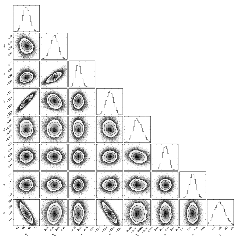
Figure 7: Marginalized contours at 68%, 95%, 99% confidence levels and posterior distributions for the parameters of the Anton-Schmidt cosmological model.

V Final outlooks and perspectives

In this paper, we proposed a new class of dark energy models, in which dark energy emerges as a consequence of the kind of barotropic factor involved for matter. We considered in Solid State Physics the case supported by isotropic deformations into crystalline solids, in which the pressure can naturally take negative values. This fact avoids to postulate a priori a negative dark energy equation of state and moreover adapts well to matter. So that, considering matter only, we model its equation of state through the Anton-Schmidt’s equation of state. Under the hypothesis that $V\propto\rho^{-1}$, we soon found that the corresponding pressure is proportional to the logarithm of universe’s volume, i.e. to the density itself. We demonstrated that a universe made of one single fluid with such a property can explain acceleration without the need of a cosmological constant. Our framework depends upon two free parameters, namely $n$ and $B$, intimately correlated with the Grüneisen parameter and the bulk modulus characterizing the typology of fluid here involved. We noticed that the acceleration process extends a class of dark energy paradigms dubbed logotropic dark fluids recently developed in the literature. We discussed the connections between these models and our model, and we showed the differences between our treatment and the concordance paradigm. Further, we related the free parameters of the CPL approach to our treatment, finding out the analogies between the two landscapes.

We highlighted the most relevant properties of the new equation of state applied to background cosmology. To fix bounds on the free parameters of our model, we employed supernova data surveys, BAO compilations and differential age measurements. We thus performed Monte Carlo computing technique implemented with the affine-invariant ensemble algorithm. In so doing, we were able to show that our alternative model candidates as a consistent alternative to dark energy and to the $\Lambda$CDM model. In particular, the concordance paradigm falls inside our approach as a limiting case.

In future works, we will analyze some open challenges of our approach. First, we will focus on better understanding the physics inside $\rho_{*}$, comparing our model with dark matter distributions. Second, we will check the goodness of our working scheme when early phases are taken into account. Last but not least, we will clarify whether the Anton-Schmidt’s equation of state is also able to produce inflationary stages of the universe, without the need of scalar fields in inflationary puzzle. Finally, we will check whether the model is capable of overcoming and passing additional experimental tests at different redshift regimes.

Appendix Experimental data compilations

In this appendix, we list the Hubble measurements and baryon acoustic oscillations data used in this work to get bounds over the free parameters of our model.

$z$	$H\pm\sigma_{H}$	Ref.
0.0708	$69.00\pm 19.68$	Zhang14
0.09	$69.0\pm 12.0$	Jimenez02
0.12	$68.6\pm 26.2$	Zhang14
0.17	$83.0\pm 8.0$	Simon05
0.179	$75.0\pm 4.0$	Moresco12
0.199	$75.0\pm 5.0$	Moresco12
0.20	$72.9\pm 29.6$	Zhang14
0.27	$77.0\pm 14.0$	Simon05
0.28	$88.8\pm 36.6$	Zhang14
0.35	$82.1\pm 4.85$	Chuang12
0.352	$83.0\pm 14.0$	Moresco16
0.3802	$83.0\pm 13.5$	Moresco16
0.4	$95.0\pm 17.0$	Simon05
0.4004	$77.0\pm 10.2$	Moresco16
0.4247	$87.1\pm 11.2$	Moresco16
0.4497	$92.8\pm 12.9$	Moresco16
0.4783	$80.9\pm 9.0$	Moresco16
0.48	$97.0\pm 62.0$	Stern10
0.593	$104.0\pm 13.0$	Moresco12
0.68	$92.0\pm 8.0$	Moresco12
0.781	$105.0\pm 12.0$	Moresco12
0.875	$125.0\pm 17.0$	Moresco12
0.88	$90.0\pm 40.0$	Stern10
0.9	$117.0\pm 23.0$	Simon05
1.037	$154.0\pm 20.0$	Moresco12
1.3	$168.0\pm 17.0$	Simon05
1.363	$160.0\pm 33.6$	Moresco15
1.43	$177.0\pm 18.0$	Simon05
1.53	$140.0\pm 14.0$	Simon05
1.75	$202.0\pm 40.0$	Simon05
1.965	$186.5\pm 50.4$	Moresco15

Table 3: Differential age $H(z)$ data used in this work. The Hubble rate is given in units of km/s/Mpc.

$z$	$d_{V}\pm\sigma_{d_{V}}$	Survey	Ref.
0.106	0.336 $\pm$ 0.015	6dFGS	Beutler11
0.15	0.2239 $\pm$ 0.0084	SDSS DR7	Ross15
0.32	0.1181 $\pm$ 0.0023	BOSS DR11	Anderson14
0.57	0.0726 $\pm$ 0.0007	BOSS DR11	Anderson14
2.34	0.0320 $\pm$ 0.0016	BOSS DR11	Delubac15
2.36	0.0329 $\pm$ 0.0012	BOSS DR11	Font-Ribera14

Table 4: BAO data used in this work.

References

- (1) S. Capozziello, M. De laurentis, O. Luongo, A. C. Ruggeri, Galaxies, 1, 216-260 (2013); P. J. E. Peebles, B. Ratra, Rev. Mod. Phys., 75, 559 (2003).
- (2) M. J. Mortonson, D. H. Weinberg, M. White, arXiv:1401.0046; P. K. S. Dunsby and O. Luongo, Int. J. Geom. Methods Mod. Phys., 13, 1630002 (2016).
- (3) S. Perlmutter et al., Nature, 391, 51-54 (1998); B. P. Schmidt et al., Astrophys. J., 507, 46-63 (1998); A. G. Riess et al., Astrophys. J., 607, 665-687 (2004).
- (4) N. Suzuki et al., Astrophys. J, 746, 85 (2012).
- (5) D. H. Weinberg, M. J. Mortonson, D. J. Eisenstein, C. Hirata, A. G. Riess, E. Rozo, Phys. Rept., 530, 87 (2013); B. Jain and J. Khoury, Annals Phys. 325, 1479 (2010).
- (6) S. Tsujikawa, arXiv:1004.1493 (2010); L. M. Krauss, J. Dent, Phys. Rev. Lett., 111, 061802 (2013).
- (7) I. Zlatev, L. M. Wang, and P. J. Steinhardt, Phys. Rev. Lett., 82, 896-899 (1999); V. Sahni and A. A. Starobinsky, Int. J. Mod. Phys. D, 9, 373 (2000); L. Amendola, M. Kunz, M. Motta, I. D. Saltas and I. Sawicki, Phys. Rev. D, 87, 023501 (2013).
- (8) E. J. Copeland, M. Sami, S. Tsujikawa, Int. J. Mod. Phys. D, 15, 1753-1936 (2006).
- (9) K. Bamba, S. Capozziello, S. Nojiri, S. D. Odintsov, Astrophys. Space Sci., 342, 155 -228 (2012).
- (10) M. D. Maia, A. J. S. Capistrano, E. M. Monte, Int. J. Mod. Phys., A24, 1545-1548 (2009); M. Li, X.-D. Li, S. Wang, Y. Wang, Frontiers of Physics, 8, 828-846 (2013).
- (11) S. Chaplygin, Sci. Mem. Moscow Univ. Math. Phys., 21, 1 (1904); A. Kamenshchik, U. Moschella, V. Pasquier, Phys. Lett. B, 511, 265 (2001).
- (12) M. C. Bento, O. Bertolami, A. A. Sen, Phys. Rev. D, 66, 043507 (2002); B. Pourhassan et al., Results Phys., 4, 101-102 (2014).
- (13) K. Arun, S. B. Gudennavar, C. Sivaram, Advances in Space Research, 60, 166-186 (2017).
- (14) H. Anton, P. C. Schmidt, Intermetallics, 5, 449-465 (1997); B. Mayer et al., Intermetallics, 11(1), 23-32 (2003).
- (15) A. L. Ivanovskii, Progress in Materials Science, 57, 1 (2012).
- (16) S. Nojiri, S. D. Odintsov, Phys. Rept., 505, 59 (2011); S. Nojiri, S. D. Odintsov, V. K. Oikonomou, Phys. Rept., 692, 1 (2017); S. Nojiri, S. D. Odintsov, Phys. Rev. D, 68, 123512 (2003).
- (17) P. H. Chavanis, Eur. Phys. J. Plus, 130, 130 (2015); P. H. Chavanis, Phys. Lett. B, 758, 59 (2016).
- (18) Gruneisen, E., Annalen der Physik, 344, 257-306 (1912).
- (19) T. H. K. Barron, Ann. Phys., 1, 77-90 (1957).
- (20) P. Debye, Annalen der Physik, 39(4): 789-839 (1912).
- (21) D. L. Anderson, Blackwell Scientific Publications, Oxford (1989).
- (22) P. J. E. Peebles, Principles of Physical Cosmology, Princeton Univ. Press (1993).
- (23) P. A. R. Ade et al. [Planck Collaboration], Astron. Astrophys, 594, A13 (2016).
- (24) P. H. Chavanis and S. Kumar, J. Cosmol. Astropart. Phys., 1705, 018 (2017).
- (25) M. Chevallier, D. Polarski, Int. J. Mod. Phys. D,10, 213-223 (2001).
- (26) E. Linder, Phys. Rev. Lett. 90, 091301 (2003).
- (27) S. Weinberg, Cosmology and Gravitation, John Wiley Sons, N.Y. (1972).
- (28) V. F. Mukhanov, H. A. Feldmanc, R. H. Brandenberger, Phys.Rept., 215, 203-333 (1992).
- (29) F. Donato et al., Mon. Not. R. Astron. Soc., 397, 1169 (2009).
- (30) A. Saburova, A. Del Popolo, Mon. Not. R. Astron. Soc., 445, 3512 (2014).
- (31) S. Weinberg, Rev. Mod. Phys., 61, 1-23 (1989); T. Padmanabhan, Phys. Rept., 380, 235-320 (2003); C. P. Burgess, arXiv:1309.4133 (2013).
- (32) M. Betoule et al., Astron. Astrophys., 568, A22 (2014).
- (33) R. Jimenez, A. Loeb, Astrophys. J., 573, 37 (2002).
- (34) V. Lukovic, R. D’Agostino, N. Vittorio, Astron. Astrophys., 595, A109 (2016).
- (35) D. J. Eisenstein et al., Astrophys. J., 633, 560-574 (2005).
- (36) D. Foreman-Mackey, D. W. Hogg, D. Lang, J. Goodman, PASP, 125, 306 (2013).
- (37) J. Goodman and J. Weare, Comm. App. Math. Comp. Sci., 5(1), 65 (2010).
- (38) M. Vargas dos Santos, R. R. Reis, I. Waga, JCAP, 1602(02), 066 (2016).
- (39) C. Zhang et al., Res. Astron. Astrophys., 14, 1221 (2014).
- (40) J. Simon, L. Verde, R. Jimenez, Phys. Rev. D, 71, 123001 (2005).
- (41) M. Moresco et al., J. Cosmol. Astropart. Phys., 8, 006 (2012).
- (42) C.-H. Chuang et al., Mon. Not. R. Astron. Soc., 426, 226 (2012).
- (43) M. Moresco et al., J. Cosmol. Astropart. Phys., 05, 014 (2016).
- (44) D. Stern, R. Jimenez, L. Verde, S. A. Stanford, M. Kamionkowski, ApJS, 188, 280 (2010).
- (45) M. Moresco, Mon. Not. R. Astron. Soc, 450, L16 (2015).
- (46) F. Beutler et al., Mon. Not. R. Astron. Soc, 416, 3017 (2011).
- (47) A. Ross et al., Mon. Not. R. Astron. Soc, 449, 835 (2015).
- (48) L. Anderson et al., Mon. Not. R. Astron. Soc, 441, 24 (2014).
- (49) T. Delubac et al., Astron. Astrophys, 574, A59 (2015).
- (50) A. Font-Ribera et al., J. Cosmology Astropart. Phys., 5, 27 (2014).